Mapping Aboveground Woody Biomass on Abandoned Agricultural Land Based on Airborne Laser Scanning Data


Abstract
1. Introduction
2. Materials and Methods
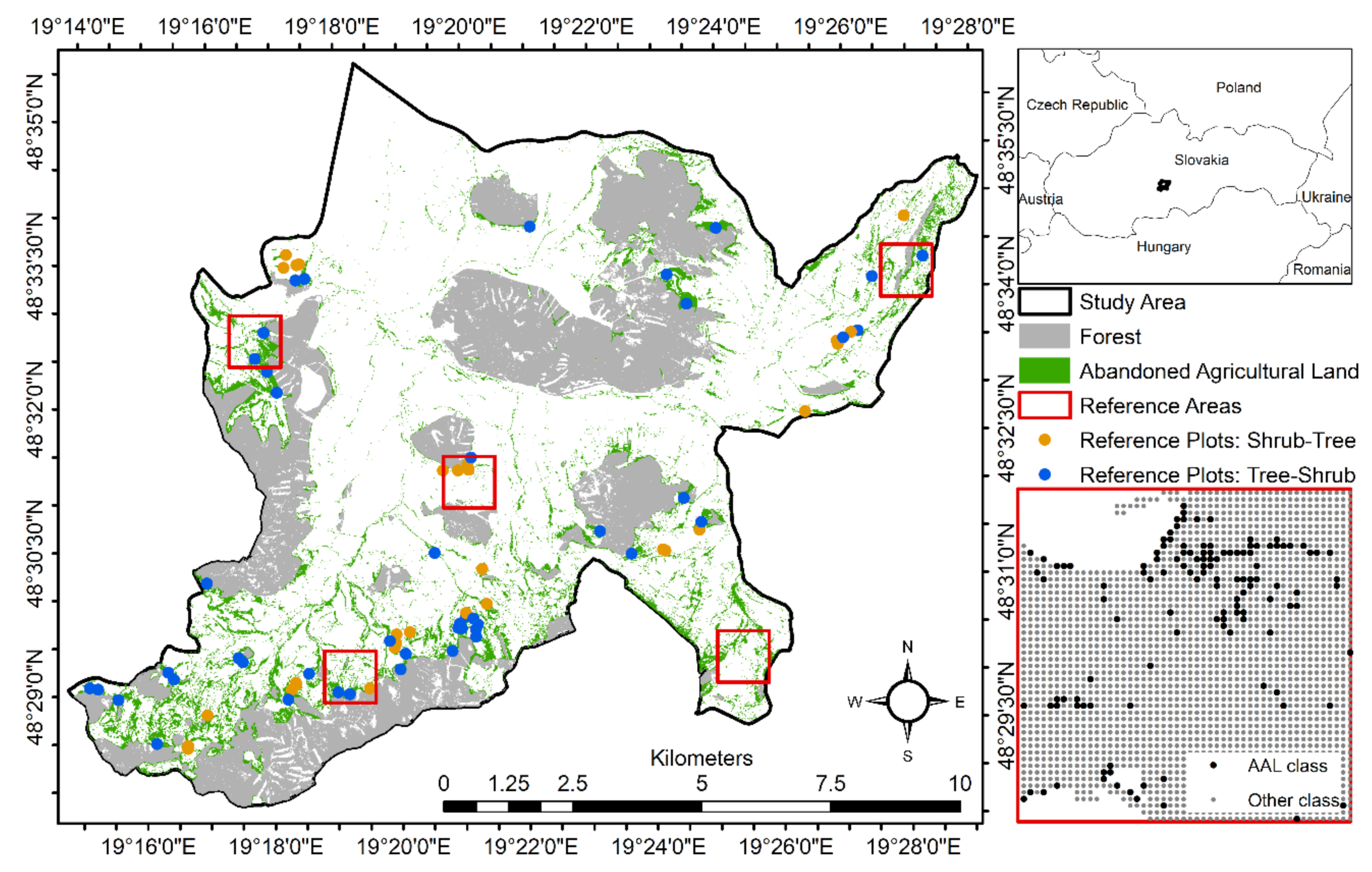
2.1. Ground Data
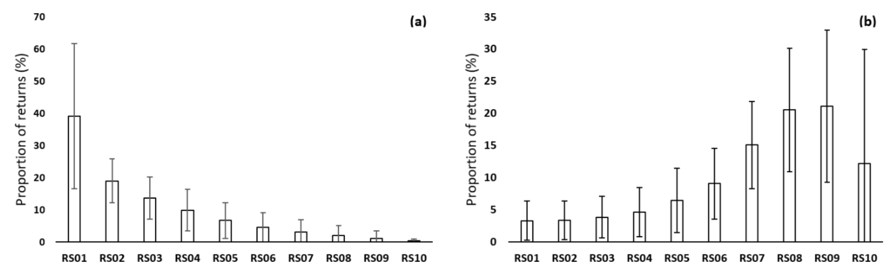
2.2. Airborne Data
2.3. Additional Geospatial Data
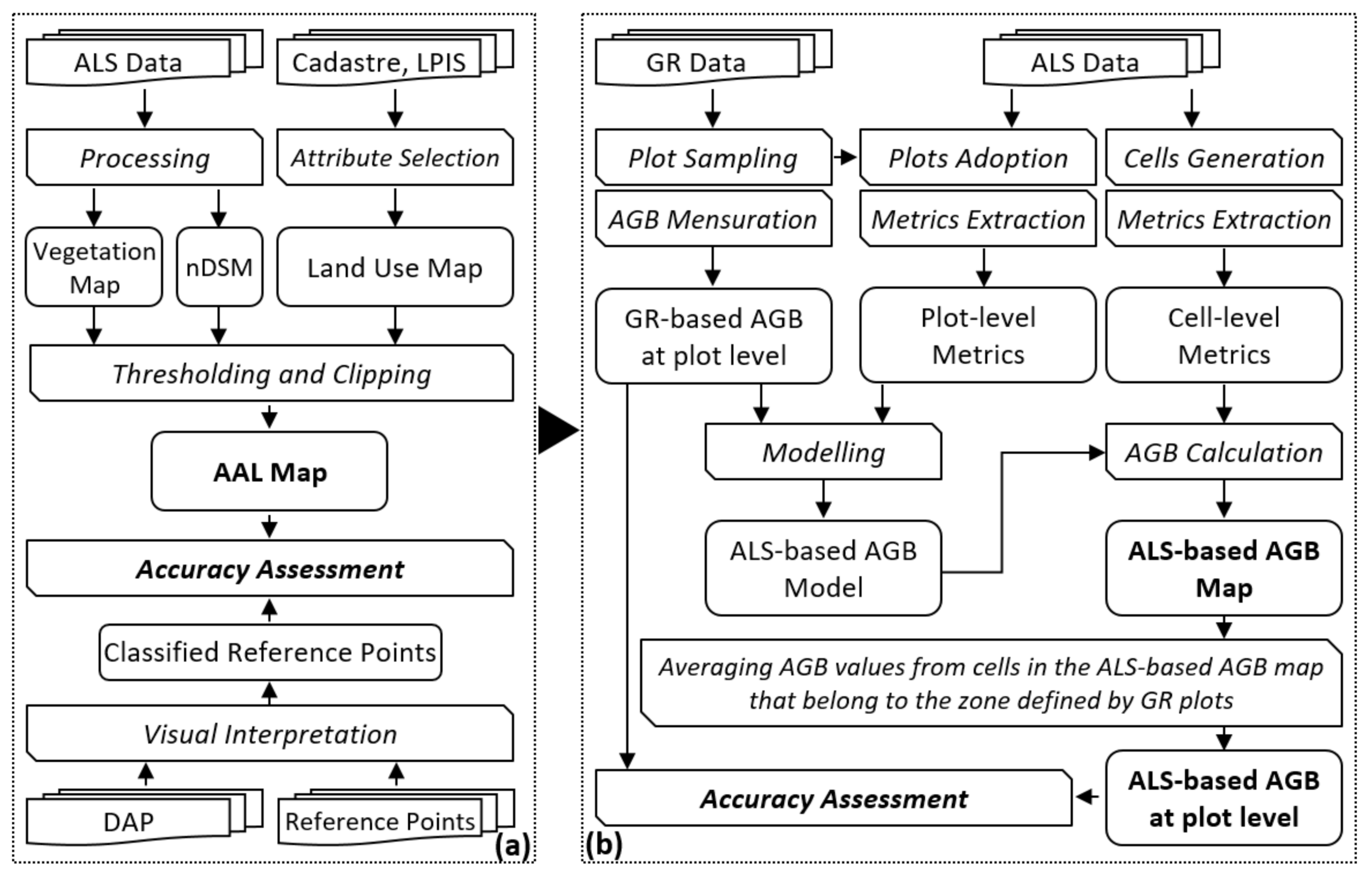
2.4. Workflow
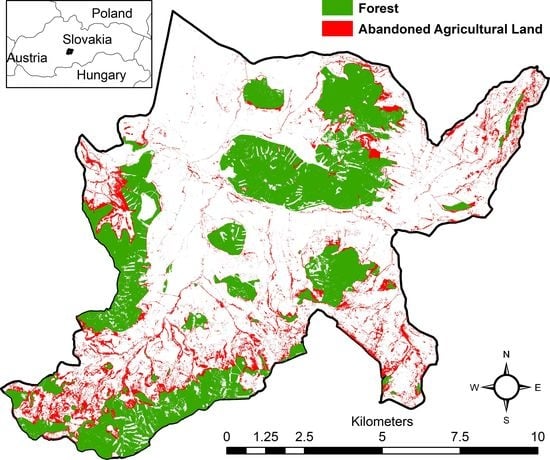
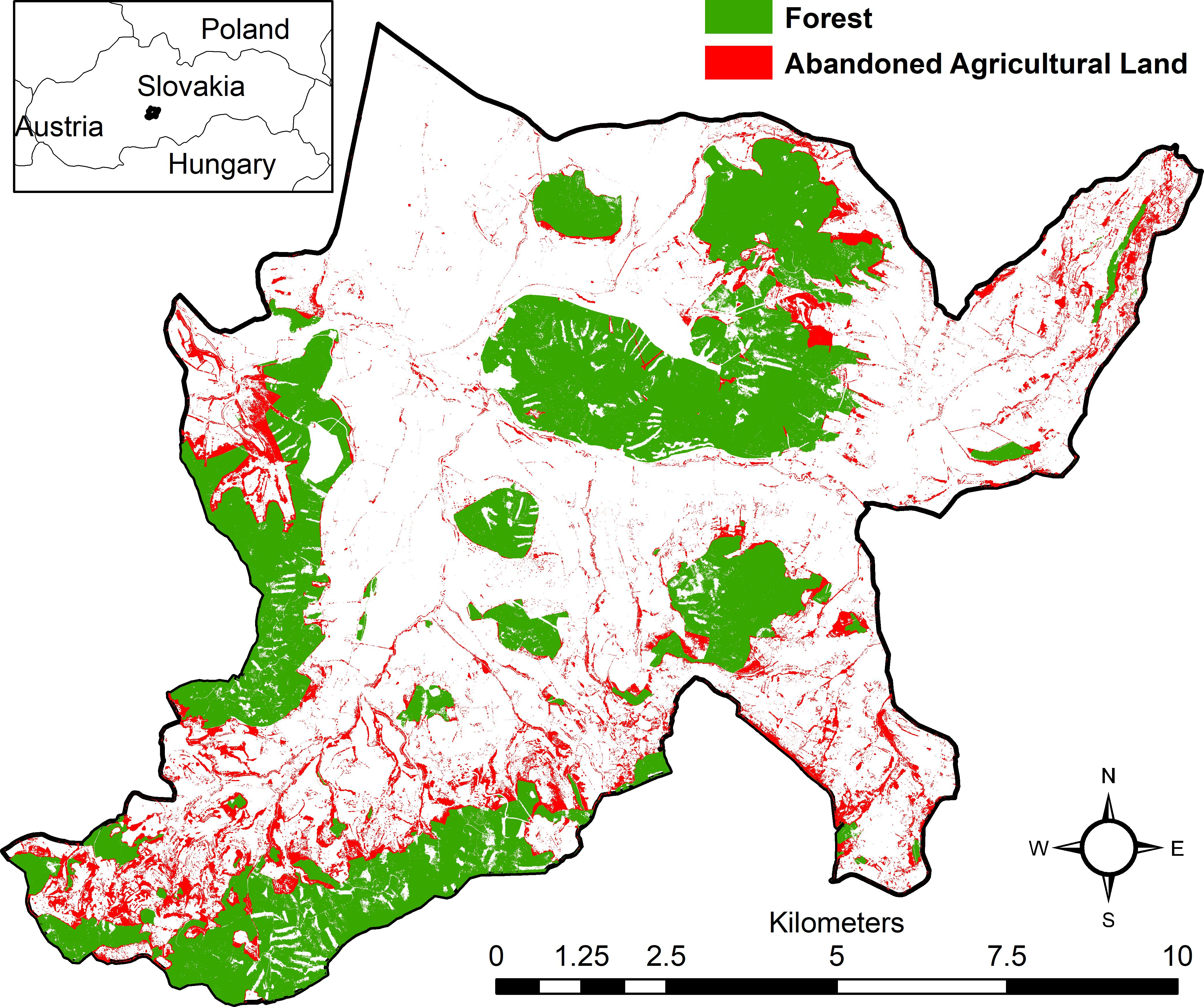
2.4.1. Spatial Identification of Abandoned Agricultural Land
2.4.2. Mapping Aboveground Woody Biomass on Abandoned Agricultural Land
2.4.3. Validation of the Models and Maps
3. Results
3.1. Performance of the Spatial Identification of Abandoned Agricultural Land
3.2. Performance of Mapping the Aboveground Woody Biomass on Abandoned Agricultural Land
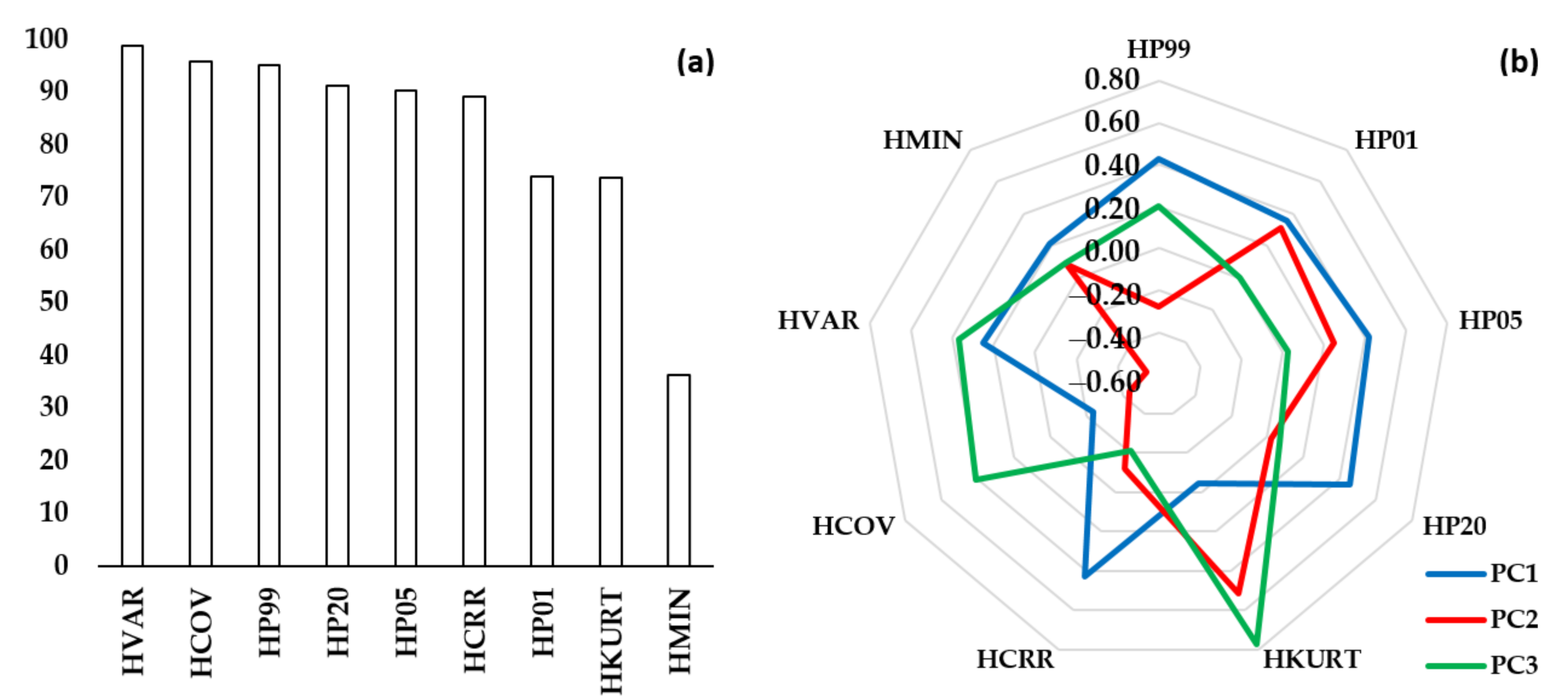
3.2.1. Predictor Variable Selection
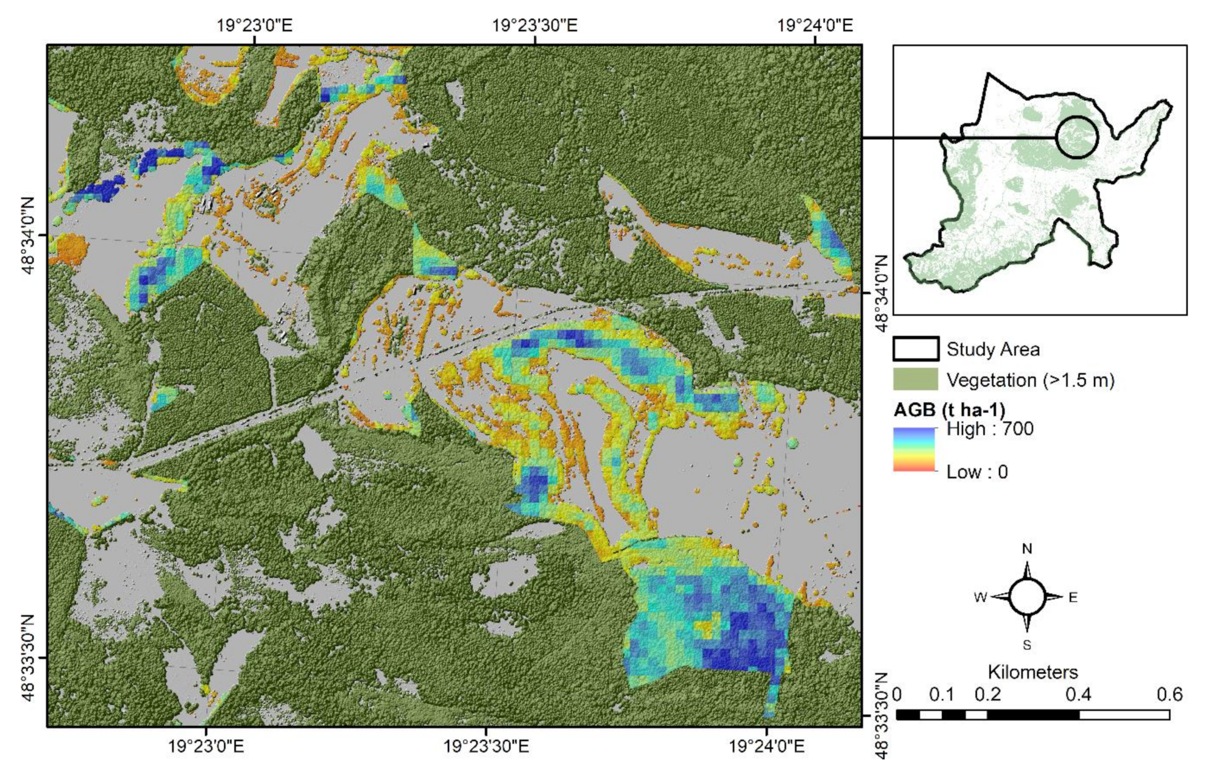
3.2.2. Accuracy of the AGB Map
4. Discussion
- (1)
- Uncontrolled cessation of agricultural production and the subsequent afforestation of agricultural land through forest succession is a serious challenge for the effective management of natural resources.
- (2)
- Mapping AGB on AAL is strictly required by relevant stakeholders (e.g., farmers, foresters, parcel owners, environmentalist, and policy-makers). This is primarily because these geospatial data make it possible to understand the state and trend of afforestation/deforestation in related regions and subsequently to implement a proper policy focused on the reduction of the negative effects of giving up agricultural production, support for sustainable forest management, or aimed at obtaining financial support.
- (3)
- RS technologies, especially ALS, represent an effective way to predict AGB on AAL and provide an opportunity to complement ground-based monitoring. Here, the ABA and RF models generally allowed us to obtain unbiased estimates of AGB and, in addition, the point density requirements of ALS data, hardware performance, and processing time are lower than with other methods.
4.1. Spatial Identification of Abandoned Agricultural Land
4.2. Mapping Aboveground Woody Biomass on Abandoned Agricultural Land
5. Conclusions
- (1)
- ALS data allowed for an automated and more accurate identification of AAL in terms of classification accuracy (>90%) and spatial resolution (<1.0 m) than did other RS platforms [53,54,55,56,57,58,59,60,61,62,63,64]. Potential improvements in process of AAL identification may be achieved using some qualitative variable of ALS data (e.g., intensity) or alternatively through multispectral ALS data [65,66,67,68]. The additional costs related to the application of ALS may be optimized by long-term survey planning.
- (2)
- Cadastral and LPIS data allowed us to apply the legal spatial status of parcels and to identify farmland without active agricultural activities. A combination of these data sources with the high-resolution ALS-derived map of vegetation resulted in more objective identification of AAL.
- (3)
- The authors’ algorithm implemented in the reFLex software was capable of providing relevant point cloud metrics (i.e., height) at the reference plot level (75 reference plots) as well as at forest management unit level (85,648 cells).
- (4)
- ALS data, despite a slight underestimation (bias from −2% to −6%), allowed more accurate prediction of AGB (RMSE < 33%) using ABA and the RF models than did other RS platforms [69,70,71,72,73,74,75]. Although the development of ecosystem-specific (e.g., tree species group and vegetation type) models is generally recommended, the single comprehensive RF model based on height metrics was sufficiently accurate for the whole area of interest (corresponding bias was not statistically significant). The additional costs related to obtaining the field data necessary for the development of the RF model may be optimized by the selection of a suitable sample design.
Author Contributions
Funding
Acknowledgments
Conflicts of Interest
References
- Alcantara, C.; Kuemmerle, T.; Prishchepov, A.V.; Radeloff, V.C. Mapping abandoned agriculture with multi-temporal MODIS satellite data. Remote Sens. Environ. 2012, 124, 334–347. [Google Scholar] [CrossRef]
- Kuemmerle, T.; Hostert, P.; Radeloff, V.C.; Van der Linden, S.; Perzanowski, K.; Kruhlov, I. Cross-border comparison of post-socialist farmland abandonment in the Carpathians. Ecosystems 2008, 11, 614–628. [Google Scholar] [CrossRef]
- Rey Benayas, J.; Martins, A.; Nicolau, J.M.; Schulz, J.J. Abandonment of agricultural land: An overview of drivers and consequences. CAB Rev. Perspect. Agric. Vet. Sci. Nutr. Nat. Resour. 2007, 2, 1–14. [Google Scholar] [CrossRef]
- Baumann, M.; Kuemmerle, T.; Elbakidze, M.; Ozdogan, M.; Radelo, V.C.; Keuler, N.S.; Prishchepov, A.V.; Kruhlov, I.; Hostert, P. Patterns and drivers of post-socialist farmland abandonment in Western Ukraine. Land Use Policy 2011, 28, 552–562. [Google Scholar] [CrossRef]
- Kumar, R.; Das, A.J. Climate change and its impact on land Degradation: Imperative need to focus. Climatol. Weather Forecast. 2014, 2, 2–4. [Google Scholar] [CrossRef]
- Goudriaan, J.; Unsworth, M.H. Impact of carbon dioxide, trace gases, and climate change on global agriculture. In Implications of Increasing Carbon Dioxide and Climate Change for Agricultural Productivity and Water Resources; Kimball, B.A., Ed.; American Society of Agronomy, Crop Society of America, and Soil Science Society of America: Madison, WI, USA, 1990; pp. 111–130. [Google Scholar]
- Queiroz, C.; Beilin, R.; Folke, C.; Lindborg, R. Farmland abandonment: Threat or opportunity for biodiversity conservation? A global review. Front. Ecol. Environ. 2014, 12, 288–296. [Google Scholar] [CrossRef]
- Goga, T.; Feranec, J.; Bucha, T.; Rusnák, M.; Sačkov, I.; Barka, I.; Kopecká, M.; Papčo, J.; Oťaheľ, J.; Szatmári, D.; et al. A review of the application of remote sensing data for abandoned agricultural land identification with focus on Central and Eastern Europe. Remote Sens. 2019, 11, 2759. [Google Scholar] [CrossRef]
- Li, W.; Wang, S.; Zhou, Y.; Xu, Q.; Wang, F.; Han, Y. Remote sensing methods for surveying and extracting abandoned farmlands. In Proceedings of the 2012 5th International Congress on Image and Signal Processing, Chongqing, China, 16–18 October 2012; pp. 1086–1090. [Google Scholar]
- Véga, C.; Renaud, J.; Durrieu, S.; Bouvier, M. On the interest of penetration depth, canopy area and volume metrics to improve Lidar-based models of forest parameters. Remote Sens. Environ. 2016, 175, 32–42. [Google Scholar] [CrossRef]
- Surový, P.; Kuželka, K. Acquisition of Forest Attributes for Decision Support at the Forest Enterprise Level Using Remote-Sensing Techniques—A Review. Forests 2019, 10, 273. [Google Scholar] [CrossRef]
- Kardoš, M.; Medveďová, A.; Supek, Š.; Škodová, M. Objektovo orientovaná klasifikácia drevinového zloženia na digitálnych leteckých snímkach zosuvného územia. Zprávy Lesnického Výzkumu 2013, 58, 195–205. (In Slovak) [Google Scholar]
- Ballanti, L.; Blesius, L.; Hines, E.; Kruse, B. Tree species classification using hyperspectral imagery: A comparison of two classifiers. Remote Sens. 2016, 8, 445. [Google Scholar] [CrossRef]
- Schlund, M.; Davidson, M.W.J. Aboveground forest biomass estimation combining L- and P-Band SAR acquisitions. Remote Sens. 2018, 10, 1151. [Google Scholar] [CrossRef]
- Brigot, G.; Simard, M.; Colin-Koeniguer, E.; Boulch, A. Retrieval of forest vertical structure from PolInSAR data by machine learning using LIDAR-derived features. Remote Sens. 2019, 11, 381. [Google Scholar] [CrossRef]
- Stefanski, J.; Chaskovskyy, O.; Waske, B. Mapping and monitoring of land use changes in post-Soviet western Ukraine using remote sensing data. Appl. Geogr 2014, 55, 155–164. [Google Scholar] [CrossRef]
- Wang, S.X.; Li, W.J.; Zhou, Y.; Wang, F.T.; Xu, Q.L. Object-oriented classification technique for extracting abandoned farmlands by using remote sensing images. In Proceedings of the 3rd International Conference on Multimedia Technology, Guangzhou, China, 29 November–1 December 2013; pp. 1497–1504. [Google Scholar]
- Yuso, N.M.; Muharam, F.M.; Takeuchi, W.; Darmawan, S.; Abd Razak, M.H. Phenology and classification of abandoned agricultural land based on ALOS-1 and 2 PALSAR multi-temporal measurements. Int. J. Digit. Earth 2017, 10, 155–174. [Google Scholar]
- Guenthert, S.; Siegmund, A.; Thunig, H.; Michel, U. Object-based detection of LUCC with special regard to agricultural abandonment on Tenerife (Canary Islands). In Proceedings of the Earth Resources and Environmental Remote Sensing/GIS Applications II, Prague, Czech Republic, 26 October 2011; Volume 8181, pp. 1–7. [Google Scholar]
- Löw, F.; Fliemann, E.; Abdullaev, I.; Conrad, C.; Lamers, J.P.A. Mapping abandoned agricultural land in Kyzyl-Orda, Kazakhstan using satellite remote sensing. Appl. Geogr. 2015, 62, 377–390. [Google Scholar] [CrossRef]
- Alcantara, C.; Kuemmerle, T.; Baumann, M.; Bragina, E.V.; Griths, P.; Hostert, P.; Knorn, J.; Müller, D.; Prishchepov, A.V.; Schierhorn, F. Mapping the extent of abandoned farmland in Central and Eastern Europe using MODIS time series satellite data. Environ. Res. Lett. 2013, 8, 035035. [Google Scholar] [CrossRef]
- Bożek, P.; Janus, J.; Mitka, B. Analysis of changes in forest structure using point clouds from historical aerial photographs. Remote Sens. 2019, 11, 2259. [Google Scholar] [CrossRef]
- Kolecka, N.; Kozak, J.; Kaim, D.; Dobosz, M.; Ostafin, K.; Ostapowicz, K.; Wezik, P.; Price, B. Understanding farmland abandonment in the polish Carpathians. Appl. Geogr. 2017, 88, 62–72. [Google Scholar] [CrossRef]
- Dube, T.; Mutanga, O.; Shoko, C.; Adelabu, S.A. Remote sensing of aboveground forest biomass: A review. Trop. Ecol. 2016, 57, 125–132. [Google Scholar]
- Barbosa, J.M.; Broadbent, E.N.; Bitencourt, M.D. Remote sensing of aboveground biomass in tropical secondary forests: A review. Int. J. For. Res. 2014, 715796, 1–14. [Google Scholar] [CrossRef]
- Li, A.; Dhakal, S.; Glenn, N.F.; Spaete, L.P.; Shinneman, D.J.; Pilliod, D.S.; Arkle, R.S.; McIlroy, S.K. Lidar aboveground vegetation biomass estimates in shrublands: Prediction, uncertainties and application to coarser scales. Remote Sens. 2017, 9, 903. [Google Scholar] [CrossRef]
- Askar, A.; Nuthammachot, N.; Phairuang, W.; Wicaksono, P.; Sayektiningsih, T. Estimating aboveground biomass on private forest using Sentinel-2 imagery. J. Sens. 2018, 2018, 1–11. [Google Scholar] [CrossRef]
- Liu, N.; Harper, R.J.; Handcock, R.N.; Evans, B.; Sochacki, S.J.; Dell, B.; Walden, L.L.; Liu, S. Seasonal timing for estimating carbon mitigation in revegetation of abandoned agricultural land with high spatial resolution remote sensing. Remote Sens. 2017, 9, 545. [Google Scholar] [CrossRef]
- Walden, L.L.; Harper, R.J.; Sochacki, S.J.; Montagu, K.D.; Wocheslander, R.; Clarke, M.; Ritson, P.; Emms, J.; Davoren, C.W.; Mowat, D.; et al. Mitigation of carbon following Atriplex nummularia revegetation in southern Australia. Ecol. Eng. 2017, 106, 253–262. [Google Scholar] [CrossRef]
- Helman, D.; Mussery, A.; Lensky, I.M.; Leu, S. Detecting changes in biomass productivity in a different land management regimes in drylands using satellite-derived vegetation index. Soil Use Manag. 2014, 30, 32–39. [Google Scholar] [CrossRef]
- Shen, W.; Li, M.; Huang, C.; Tao, X.; Li, S.; Wei, A. Mapping annual forest change due to afforestation in Guangdong province of China using active and passive remote sensing data. Remote Sens. 2019, 11, 490. [Google Scholar] [CrossRef]
- Maltamo, M.; Naesset, E.; Vauhkonen, J. Forestry Application of Airborne Laser Scanning: Concept and Case Studies; Springer: Dordrecht, The Netherlands, 2014; p. 460. [Google Scholar]
- Shinzato, E.T.; Shimabukuro, Y.E.; Coops, N.C.; Tompalski, P.; Gasparoto, E.A.G. Integrating area-based and individual tree detection approaches for estimating tree volume in plantation inventory using aerial image and airborne laser scanning data. iForest 2016, 10, 296–302. [Google Scholar] [CrossRef]
- Mauro, F.; Ritchie, M.; Wing, B.; Frank, B.; Monleon, V.; Temesgen, H.; Hudak, A. Estimation of changes of forest structural attributes at three different spatial aggregation levels in northern California using multitemporal LiDAR. Remote Sens. 2019, 11, 923. [Google Scholar] [CrossRef]
- Sibona, E.; Vitali, A.; Meloni, F.; Caffo, L.; Dotta, A.; Lingua, E.; Motta, R.; Garbarino, M. Direct measurement of tree height provides different results on the assessment of LiDAR accuracy. Forests 2017, 8, 7. [Google Scholar] [CrossRef]
- USDA Forest Services: FUSION/LDV LIDAR Analysis and Visualization Software. Available online: http://forsys.cfr.washington.edu/FUSION/fusion_overview.html (accessed on 18 August 2020).
- Rapidlasso GmbH: Fast Tools to Catch Reality. Available online: https://rapidlasso.com (accessed on 18 August 2020).
- Sačkov, I.; Hlásny, T.; Bucha, T.; Juriš, M. Integration of tree allometry rules to treetops detection and tree crowns delineation using airborne lidar data. iForest 2017, 10, 459–467. [Google Scholar] [CrossRef]
- Sačkov, I.; Kulla, L.; Bucha, T. A Comparison of Two Tree Detection Methods for Estimation of Forest Stand and Ecological Variables from Airborne LiDAR Data in Central European Forests. Remote Sens. 2019, 11, 1431. [Google Scholar] [CrossRef]
- Iizuka, K.; Hayakawa, Y.S.; Ogura, T.; Nakata, Y.; Kosugi, Y.; Yonehara, T. Integration of multi-sensor data to estimate plot-level stem volume using machine learning algorithms–case study of evergreen conifer planted forests in Japan. Remote Sens. 2020, 12, 1649. [Google Scholar] [CrossRef]
- Santopuoli, G.; Di Febbraro, M.; Maesano, M.; Balsi, M.; Marchetti, M.; Lasserre, B. Machine Learning Algorithms to predict tree-related microhabitats using airborne laser scanning. Remote Sens. 2020, 12, 2142. [Google Scholar] [CrossRef]
- Silva, V.S.; Silva, C.A.; Mohan, M.; Cardil, A.; Rex, F.E.; Loureiro, G.H.; Almeida, D.R.A.; Broadbent, E.N.; Gorgens, E.B.; Dalla Corte, A.P.; et al. Combined impact of sample size and modeling approaches for predicting stem volume in eucalyptus spp. forest plantations using field and LiDAR data. Remote Sens. 2020, 12, 1438. [Google Scholar] [CrossRef]
- Murgaš, V.; Sačkov, I.; Sedliak, M.; Tunák, D.; Chudý, F. Assessing horizontal accuracy of inventory plots in forests with different mix of tree species composition and development stage. J. For. Sci. 2018, 64, 478–485. [Google Scholar] [CrossRef]
- Petráš, R.; Pajtík, J. Sústava česko-slovenských objemových tabuliek drevín. Lesnícky Časopis 1991, 37, 49–56. (In Slovak) [Google Scholar]
- Konôpka, B.; Pajtík, J.; Šebeň, V. Biomass functions and expansion factors for young trees of European ash and Sycamore maple in the Inner Western Carpathians. Austrian J. For. Sci. 2015, 132, 1–26. [Google Scholar]
- EU. The Land Parcel Identification System: A Useful Tool to Determine the Eligibility of Agricultural Land–but Its Management could Be Further Improved. Special Report No. 25. 2016. Available online: https://op.europa.eu/en/publication-detail/-/publication/11049e0e-9a82-11e6-9bca-01aa75ed71a1 (accessed on 18 August 2020).
- ASPRS. LAS Specification 1.4. Available online: http://www.asprs.org/wp-content/uploads/2019/03/LAS14r14.pdf (accessed on 18 August 2020).
- INPHO. SCOP++. Available online: http://trl.trimble.com/docushare/dsweb/Get/Document-696440/022516-022B_Inpho_SCOP___TS_USL_0516_LR.pdf (accessed on 18 August 2020).
- FAO. FAOSTAT: Methods & Standards. Available online: http://www.fao.org/ag/agn/nutrition/Indicatorsfiles/Agriculture.pdf (accessed on 18 August 2020).
- Pointereau, P.; Coulon, F.; Girard, P.; Lambotte, M.; Stuczynski, T.; Sanchez Ortega, V.; Del Rio, A. Analysis of farmland abandonment and the extent and location of agricultural areas that are actually abandoned or are in risk to be abandoned. In JCR Scientific and Technical Reports; European Commission Joint Research Centre, Institute for Environment and Sustainability Press: Luxembourg, 2008. [Google Scholar]
- Perpiña, C.C.; Kavalov, B.; Diogo, V.; Jacobs-Crisioni, C.; Batista e Silva, F.; Lavalle, C. Agricultural Land Abandonment in the EU within 2015–2030; JRC113718; European Commission: Ispra, Italy, 2018; p. 7. [Google Scholar]
- Liaw, A.; Wiener, M. Classification and regression by random forest. R News 2002, 2, 18–22. [Google Scholar]
- Breiman, L. Random forests. Mach. Learn. 2001, 45, 5–32. [Google Scholar] [CrossRef]
- Eriksson, L.; Byrne, T.; Johansson, E.; Trygg, J.; Vikström, C. Multi- and Megavariate Data Analysis: Basic Principles and Applications; MKS Umetrics AB: Malmo, Sweden, 2013; p. 490. [Google Scholar]
- Kerr, G.H.G.; Fischer, C.; Reulke, R. Reliability assessment for remote sensing data: Beyond Cohen’s kappa. In Proceedings of the IEEE International Geoscience and Remote Sensing Symposium (IGARSS), Milan, Italy, 26–31 July 2015; pp. 141–152. [Google Scholar]
- Bożek, P.; Janus, J.; Taszakowski, J.; Głowacka, A. The use of Lidar data and cadastral databases in the identification of land abandonment. In Proceedings of the 17th International Multidisciplinary Scientific GeoConference SGEM, Vienna, Austria, 27–29 November 2017; pp. 705–712. [Google Scholar]
- Bożek, P.; Janus, J.; Lapa, P. The influence of the canopy height model methodology on determining abandoned agricultural areas. In Proceedings of the 17th International scientific conference Engineering for rural development, Jeglava, Latvia, 23–25 May 2018; pp. 795–800. [Google Scholar]
- Janus, J.; Bożek, P. Using ALS data to estimate afforestation and secondary forest succession on agricultural areas: An approach to improve the understanding of land abandonment causes. Appl. Geogr. 2018, 97, 128–141. [Google Scholar] [CrossRef]
- Hellesen, T.; Matikainen, L. An object-based approach for mapping shrub and tree cover on grassland habitats by use of LiDAR and CIR orthoimages. Remote Sens. 2013, 5, 558–583. [Google Scholar] [CrossRef]
- Morell-Monzó, S.; Estornell, J.; Sebastiá-Frasquet, M.T. Comparison of Sentinel-2 and high-resolution imagery for mapping land abandonment in fragmented areas. Remote Sens. 2020, 12, 2062. [Google Scholar] [CrossRef]
- Sun, B.; Gao, Z.; Zhao, L.; Wang, H.; Gao, W.; Zhang, Y. Extraction of information on trees outside forests based on very high spatial resolution remote sensing images. Forests 2019, 10, 835. [Google Scholar] [CrossRef]
- Liang, X.; Li, Y.; Zhou, Y. Study on the abandonment of sloping farmland in Fengjie County, Three Gorges Reservoir Area, a mountainous area in China. Land Use Policy 2020, 97, 104760. [Google Scholar] [CrossRef]
- Song, W. Mapping cropland abandonment in mountainous areas using an annual land-use trajectory approach. Sustainability 2019, 11, 5951. [Google Scholar] [CrossRef]
- Gašparović, M.; Dobrinić, D. Comparative Assessment of Machine Learning Methods for Urban Vegetation Mapping Using Multitemporal Sentinel-1 Imagery. Remote Sens. 2020, 12, 1952. [Google Scholar] [CrossRef]
- Goga, T.; Szatmári, D.; Feranec, J.; Papčo, J. Abandoned agricultural land identification using object-based approach and Sentinel data in the Danubian lowland, Slovakia. Int. Arch. Photogramm. Remote Sens. Spat. Inf. Sci. 2020, XLIII-B3-2020, 1539–1545. [Google Scholar] [CrossRef]
- Kolecka, N.; Kozak, J.; Kaim, D.; Dobosz, M.; Ginzler, C.; Psomas, A. Mapping secondary forest succession on abandoned agricultural land with LiDAR point clouds and terrestrial photography. Remote Sens. 2015, 7, 8300–8322. [Google Scholar] [CrossRef]
- Yan, W.Y.; Shaker, A.; El-Ashmawy, N. Urban land cover classification using airborne LiDAR data: A review. Remote Sens. Environ. 2015, 158, 295–310. [Google Scholar] [CrossRef]
- Ekhtari, N.; Glennie, C.; Fernandez-Diaz, J.C. Classification of airborne multispectral LiDAR point clouds for land cover mapping. IEEE J. Sel. Top. Appl. Earth Obs. Remote Sens. 2018, 11, 2068–2078. [Google Scholar] [CrossRef]
- Matikainen, L.; Karila, K.; Hyyppä, J.; Litkey, P.; Puttonen, E.; Ahokas, E. Object-based analysis of multispectral airborne laser scanner data for land cover classification and map updating. ISPRS J. Photogramm. Remote Sens. 2017, 128, 298–313. [Google Scholar] [CrossRef]
- Goodbody, T.R.; Tompalski, P.; Coops, N.C.; Hopkinson, C.; Treitz, P.; van Ewijk, K. Forest inventory and diversity attribute modelling using structural and intensity metrics from multi-spectral airborne laser scanning data. Remote Sens. 2020, 12, 2109. [Google Scholar] [CrossRef]
- Zhang, Z.; Cao, L.; She, G. Estimating forest structural parameters using canopy metrics derived from airborne LiDAR data in subtropical forests. Remote Sens. 2017, 9, 940. [Google Scholar] [CrossRef]
- Novo-Fernández, A.; Barrio-Anta, M.; Recondo, C.; Cámara-Obregón, A.; López-Sánchez, C.A. Integration of National Forest Inventory and Nationwide Airborne Laser Scanning Data to Improve Forest Yield Predictions in North-Western Spain. Remote Sens. 2019, 11, 1693. [Google Scholar] [CrossRef]
- Xie, B.; Cao, C.; Xu, M.; Bashir, B.; Singh, R.P.; Huang, Z.; Lin, X. Regional forest volume estimation by expanding LiDAR samples using multi-sensor satellite data. Remote Sens. 2020, 12, 360. [Google Scholar] [CrossRef]
- Sagang, L.B.T.; Ploton, P.; Sonké, B.; Poilvé, H.; Couteron, P.; Barbier, N. Airborne lidar sampling pivotal for accurate regional AGB predictions from multispectral images in forest-savanna landscapes. Remote Sens. 2020, 12, 1637. [Google Scholar] [CrossRef]
- Saarela, S.; Grafström, A.; Ståhl, G.; Kangas, A.; Holopainen, M.; Tuominen, S.; Nordkvist, K.; Hyyppä, J. Model-assisted estimation of growing stock volume using different combinations of LiDAR and Landsat data as auxiliary information. Remote Sens. Environ. 2015, 158, 431–440. [Google Scholar] [CrossRef]
- Puliti, S.; Saarela, S.; Gobakken, T.; Stahl, G.; Næsset, E. Combining UAV and Sentinel-2 auxiliary data for forest growing stock volume estimation through hierarchical model-based inference. Remote Sens. Environ. 2018, 204, 485–497. [Google Scholar] [CrossRef]
- Peters, D.L.; Niemann, K.O.; Skelly, R. Remote Sensing of Ecosystem Structure: Fusing Passive and Active Remotely Sensed Data to Characterize a Deltaic Wetland Landscape. Remote Sens. 2020, 12, 3819. [Google Scholar] [CrossRef]
- Plakman, V.; Janssen, T.; Brouwer, N.; Veraverbeke, S. Mapping Species at an Individual-Tree Scale in a Temperate Forest, Using Sentinel-2 Images, Airborne Laser Scanning Data, and Random Forest Classification. Remote Sens. 2020, 12, 3710. [Google Scholar] [CrossRef]
- Durante, P.; Martín-Alcón, S.; Gil-Tena, A.; Algeet, N.; Tomé, J.L.; Recuero, L.; Palacios-Orueta, A.; Oyonarte, C. Improving Aboveground Forest Biomass Maps: From High-Resolution to National Scale. Remote Sens. 2019, 11, 795. [Google Scholar] [CrossRef]
- Millard, K.; Richardson, M. On the importance of training data sample selection in random forest image classification: A Case Study in Peatland Ecosystem Mapping. Remote Sens. 2015, 7, 8489–8515. [Google Scholar] [CrossRef]


| Samples | n | A (ha) | Canopy Height (m) | AGB (t ha−1) | ||
|---|---|---|---|---|---|---|
| Mean | Std | Mean | Std | |||
| All plots | 75 | 2.36 | 15.38 | 13.67 | 231.51 | 221.73 |
| Shrub-tree plots * | 30 | 0.94 | 9.33 | 8.66 | 41.09 | 18.85 |
| Tree-shrub plots * | 45 | 1.42 | 36.00 | 3.56 | 358.45 | 203.09 |
| Vegetation Form | Model Form | n | A (m2) | R2 | %RMSE | p-Value |
|---|---|---|---|---|---|---|
| Shrubs species | AGB = 1.2417 × h1.45361 | 20 | 80.0 | 0.81 | 23.94 | <0.001 |
| Variable | Description | Variable | Description |
|---|---|---|---|
| HMIN | Height minimum | HVAR | Height variance |
| HMAX | Height maximum | HSTD | Height standard deviation |
| HRAN | Height range (H90-H10) | HCOV | Height coefficient of variation |
| HCRR | Canopy relief ratio (HMEAN-HMIN)/(HMAX-HMIN) | HSKEW | Height skewness |
| HMEAN | Height mean | HKURT | Height kurtosis |
| HMOD | Height mode | HP01-99 | Height 1st–99th percentile |
| Reference Data | |||||
|---|---|---|---|---|---|
| Classification | Class | AAL | Other | Total | User’s Accuracy (%) |
| AAL | 2672 | 276 | 2948 | 90.64 | |
| Other | 508 | 7738 | 8246 | 93.84 | |
| Total | 3180 | 8014 | 11,194 | ||
| Producer’s Accuracy (%) | 84.03 | 96.56 | 93.00 | ||
| Producer’s Accuracy: 90.29%; User’s Accuracy: 92.24%; Overall Accuracy: 93.00%; Cohen’s Kappa: 0.82. | |||||
| HMIN | HCRR | HVAR | HCOV | HKURT | HP01 | HP05 | HP20 | HP99 | |
|---|---|---|---|---|---|---|---|---|---|
| HMIN | 1 | ||||||||
| HCRR | 0.26 * | 1 | |||||||
| HVAR | 0.17 | 0.50 *** | 1 | ||||||
| HCOV | −0.18 | −0.46 *** | 0.11 | 1 | |||||
| HKURT | −0.10 | −0.28 * | −0.26 * | −0.15 | 1 | ||||
| HP01 | 0.37 ** | 0.56 *** | 0.10 | −0.46 *** | 0.12 | 1 | |||
| HP05 | 0.41 *** | 0.74 *** | 0.21 | −0.54 *** | 0.12 | 0.85 *** | 1 | ||
| HP20 | 0.35 ** | 0.89 *** | 0.49 *** | −0.49 *** | −0.01 | 0.69 *** | 0.88 *** | 1 | |
| HP99 | 0.33 ** | 0.85 *** | 0.80 *** | −0.20 | −0.18 | 0.52 *** | 0.70 *** | 0.89 *** | 1 |
| Samples | n | %bias | %RMSE | Normality Test | Paired Test | ||
|---|---|---|---|---|---|---|---|
| W | p-Value | Z | p-Value | ||||
| All plots | 75 | −1.93 | 26.05 | 0.72 | 0.00 | 0.56 | 0.57 |
| Shrub–tree plots | 30 | −5.57 | 33.05 | 0.92 | 0.04 | 0.34 | 0.73 |
| Tree–shrub plots | 45 | −2.43 | 21.32 | 0.78 | 0.00 | 0.02 | 0.98 |
Publisher’s Note: MDPI stays neutral with regard to jurisdictional claims in published maps and institutional affiliations. |
© 2020 by the authors. Licensee MDPI, Basel, Switzerland. This article is an open access article distributed under the terms and conditions of the Creative Commons Attribution (CC BY) license (http://creativecommons.org/licenses/by/4.0/).
Share and Cite
Sačkov, I.; Barka, I.; Bucha, T. Mapping Aboveground Woody Biomass on Abandoned Agricultural Land Based on Airborne Laser Scanning Data. Remote Sens. 2020, 12, 4189. https://doi.org/10.3390/rs12244189
Sačkov I, Barka I, Bucha T. Mapping Aboveground Woody Biomass on Abandoned Agricultural Land Based on Airborne Laser Scanning Data. Remote Sensing. 2020; 12(24):4189. https://doi.org/10.3390/rs12244189
Chicago/Turabian StyleSačkov, Ivan, Ivan Barka, and Tomáš Bucha. 2020. "Mapping Aboveground Woody Biomass on Abandoned Agricultural Land Based on Airborne Laser Scanning Data" Remote Sensing 12, no. 24: 4189. https://doi.org/10.3390/rs12244189
APA StyleSačkov, I., Barka, I., & Bucha, T. (2020). Mapping Aboveground Woody Biomass on Abandoned Agricultural Land Based on Airborne Laser Scanning Data. Remote Sensing, 12(24), 4189. https://doi.org/10.3390/rs12244189