Article

Measurement of Forest Inventory Parameters with Apple iPad Pro and Integrated LiDAR Technology

Department of Forest- and Soil Sciences, Institute of Forest Growth, University of Natural Resources and Life Sciences (BOKU), 1180 Vienna, Austria
*
Author to whom correspondence should be addressed.
Remote Sens. 2021, 13(16), 3129; https://doi.org/10.3390/rs13163129
Submission received: 22 July 2021 / Revised: 3 August 2021 / Accepted: 5 August 2021 / Published: 7 August 2021

Abstract

:
The estimation of single tree and complete stand information is one of the central tasks of forest inventory. In recent years, automatic algorithms have been successfully developed for the detection and measurement of trees with laser scanning technology. Nevertheless, most of the forest inventories are nowadays carried out with manual tree measurements using traditional instruments. This is due to the high investment costs for modern laser scanner equipment and, in particular, the time-consuming and incomplete nature of data acquisition with stationary terrestrial laser scanners. Traditionally, forest inventory data are collected through manual surveys with calipers or tapes. Practically, this is both labor and time-consuming. In 2020, Apple implemented a Light Detection and Ranging (LiDAR) sensor in the new Apple iPad Pro (4th Gen) and iPhone Pro 12. Since then, access to LiDAR-generated 3D point clouds has become possible with consumer-level devices. In this study, an Apple iPad Pro was tested to produce 3D point clouds, and its performance was compared with a personal laser scanning (PLS) approach to estimate individual tree parameters in different forest types and structures. Reference data were obtained by traditional measurements on 21 circular forest inventory sample plots with a 7 m radius. The tree mapping with the iPad showed a detection rate of 97.3% compared to 99.5% with the PLS scans for trees with a lower diameter at a breast height (dbh) threshold of 10 cm. The root mean square error (RMSE) of the best dbh measurement out of five different dbh modeling approaches was 3.13 cm with the iPad and 1.59 cm with PLS. The data acquisition time with the iPad was approximately 7.51 min per sample plot; this is twice as long as that with PLS but 2.5 times shorter than that with traditional forest inventory equipment. In conclusion, the proposed forest inventory with the iPad is generally feasible and achieves accurate and precise stem counts and dbh measurements with efficient labor effort compared to traditional approaches. Along with future technological developments, it is expected that other consumer-level handheld devices with integrated laser scanners will also be developed beyond the iPad, which will serve as an accurate and cost-efficient alternative solution to the approved but relatively expensive TLS and PLS systems. Such a development would be mandatory to broadly establish digital technology and fully automated routines in forest inventory practice. Finally, high-level progress is generally expected for the broader scientific community in forest ecosystem monitoring, as the collection of highly precise 3D point cloud data is no longer hindered by financial burdens.

1. Introduction

Forest inventories are usually carried out with fixed area plots or using the angle count sampling method. The tree positions and the diameters at breast height (dbh) are the most relevant measures with both methods. Traditional field work in forest inventories [1,2,3,4] to obtain tree positions and dbh measurements is labor-intensive, time-consuming, and prone to manifold measurement errors [5,6,7]. To overcome these problems, the combination of terrestrial inventory and modern laser sensors has been widely studied in recent decades [8]. However, manual field measures are still mandatory to calibrate and validate the models and routines that use remote sensing data as auxiliary information. The further development of efficient inventory tools is a well-known challenge related to in situ forest measurements [9]. Thus, techniques, instruments, and protocols have been permanently enhanced since the beginning of regular forest inventories 100 years ago [6].
Methods to provide 3D models of the environment have been widely used in various disciplines. When applied to forestry, laser scanning and photogrammetric methods (both airborne and terrestrial) provide valuable information for decision-making in forest management practice [10]. Forest attributes can be accurately and automatically derived from the point clouds achieved with terrestrial laser scanning (TLS) (e.g., [5,7,9,11,12,13,14,15,16,17,18,19,20,21,22]), aerial images (e.g., [8,9,23,24,25,26,27,28,29]), airborne laser scanning (ALS) (e.g., [30,31,32,33,34]), unmanned aerial vehicle (UAV) laser scanning (ULS) (e.g., [35,36,37,38,39,40]), and UAV images (e.g., [36,40,41,42,43]). With the aerial methods, it is possible to survey larger forest areas (up to the regional level) and to sample data from smaller vegetation gaps. However, especially in dense stands, ALS and UAV (except under canopy UAV) solutions were often not suitable to measure individual tree parameters, such as the tree location, dbh, and further diameters along the stem axis. This is mainly due to the lower point cloud density of the aerial approaches and because the crown canopy hinders the laser scanner from measurements of the below-foliage stem parts [44,45]. Mobile laser scanning (MLS) and personal laser scanning (PLS) have been increasingly used in recent studies, as both achieve more precise measures of the complete forest structure through the full scan across the vertical axis. In particular, MLS and PLS required only a short overall scan time and were even applicable in difficult terrain [9,44,46,47,48,49,50,51]. Hence, the efficiency of forest data collection via laser scanning has drastically improved since MLS and PLS were introduced. In contrast, the labor effort with TLS is often much higher than with MLS and PLS, especially when TLS is used in a multi-scan mode [14]. The same applies to close-range photogrammetry, which usually requires the collection of a vast number of photos from as many positions as possible. Thus far, the high labor effort associated with the measurement and co-registration of TLS and photogrammetry data, as well as the high instrument costs of the laser scanners, has prevented the existing remote sensing approaches from becoming prevalent in field measures forest inventory practice.
In 2014, Google (Google Inc., Menlo Park, CA, USA) released the first versions of devices related to “Project Tango”. The Tango technology is mainly presented as a solution for augmented reality (AR) applications, indoor measurements, and navigation. However, it can also provide useful data for a much wider area of applications, such as individual tree measurement in a forestry context (e.g., [10,52]). Constructed as integrated systems, Tango-supported devices enable the collection of 3D data on mobile platforms using sensor integration and a Simultaneous Localization and Mapping technology (SLAM, e.g., [53,54]) for the registration in 3D [52]. The measuring range of Tango depends on the depth sensor and is up to 4 m. In 2010, Microsoft (Microsoft Corporation, Redmond, WA, USA) commercialized “Kinect” as an accessory for the Xbox 360 game console. Microsoft Kinetic is a structured light system that can be operated with ordinary and low-cost consumer devices. Under optimal conditions, Kinect is able to capture several million data points per second [52]. The maximum measurement range is 4 m. Besides offering the gaming sector an augmented reality context, Kinetic was successfully connected with other applications, such as indoor mapping or forest measurements (e.g., [52,55,56,57]). A benefit of Kinect is that it efficiently brings 3D data capturing to a standard personal computer (PC), thus allowing application development [52]. Overall, Tango and Kinect (with appropriate software) technologies currently combine known approaches of SLAM with the application of RGB-D sensors and are similar in their functionality. Whereas Kinect [58,59] runs on standard PCs, laptops, and tablet PCs, Tango is a fully integrated mobile software system that runs only on a limited series of mobile devices (e.g., [60]) with an integrated depth camera.
Thus far, only a few studies on the use of such easy-to-use and low-cost consumer-level devices exist for the measurement of individual tree 3D information in a forest inventory context. The major findings of recent studies are described as follows. Tomaštík et al. [10] tested the position and dbh accuracy of Google Tango technology on circular sample plots with two different scanning walk patterns. The RMSE of the tree position finding was 1.14 m for a spiral scanning pattern and 0.20 m for a sun scanning pattern using total station data as a reference. Dbh measurement was accomplished with RMSEs of 1.91 cm and 1.15 cm using the spiral and sun scanning pattern, respectively. By using Microsoft Kinect, Brouwer [57] was able to detect all tree positions in deciduous and coniferous stand types, but the detection rates were 60% and 75% in mixed and shrub forest stands, respectively. The associated RMSE of the dbh estimation was 0.69 cm, 0.24 cm, 3.92 cm, and 0.33 cm for the different stand types, respectively. Hyyppä et al. [52] evaluated Microsoft Kinect and Google Tango against conventionally tape diameter measurements for individual tree stems. The bias of the diameter measurements was 0.54 cm (2.07%) for Kinect and 0.33 cm (0.85%) for Tango; the corresponding RMSE was 1.90 cm (7.30%) and 0.73 cm (1.89%), respectively.
A fundamental problem with the RGB-D sensors is that they are highly affected by lighting conditions. Thus, general usability under the variable natural light in outdoor applications is actually not possible, especially as it is simply not feasible to spend extra waiting time on a sample plot until acceptable and stable lighting conditions are achieved. In 2020, Apple (Apple Inc., Cupertino, CA, USA) introduced a “Light Detection And Ranging” (LiDAR)-based depth sensor and enhanced augmented reality (AR) application programming interface (API) to the 2020 iPad Pro [61] and iPhone 12 Pro [62]. LiDAR is only slightly affected by lighting conditions; thus, 3D scanning under variable natural light in outdoor applications is now possible with these devices. Thus far, only very few publications exist (e.g., [63,64]) on the performance of this new sensor and its possible application areas.
The aim of the present study was to investigate and provide initial results on the accuracy of forest inventory variables obtained by a new consumer-level mobile device, namely, the Apple 2020 iPad Pro (Apple Inc., Cupertino, CA, USA) [61], under various stand and terrain conditions. To the best of our knowledge, this is the first study on the application of this new scanner in a forest inventory context. The results of the iPad data were compared with results from PLS on the same inventory plots and using the same algorithms to produce the automatic digital terrain model (DTM) to detect the tree positions and to estimate the stem diameters. Manual individual tree measurements on the sample plots were used as reference data. In addition, indoor scans of non-wood cylindrical reference objects were performed to evaluate the iPad’s point cloud quality and to examine the accuracy of the diameter measurement with the iPad and PLS under constant in vitro conditions without possible disturbances through solar or weather conditions.
The point clouds, reference data, and application videos created for this study are made freely available (Creative Commons Attribution 4.0 International License—CC BY 4.0) under doi:10.5281/zenodo.5070671 (https://doi.org/10.5281/zenodo.5070671).

2. Materials and Methods

2.1. Study Area and Sample Plots

The study site is located in the training and research area of the University of Natural Resources and Life Science Vienna near the village of Forchtenstein, Austria, where the Institute of Forest Growth maintains a permanently repeated measures forest inventory [65]. On a total number of 554 sample plots, Bitterlich angle count sampling [66,67,68] was carried out with a constant basal area factor of k = 4 m2 ha−1. Various subsamples of the 554 points have already been used in other studies [14,15,50] to evaluate PLS and TLS approaches in a forest inventory context, as the Forchtenstein study area provides a large heterogeneity in the terrain characteristics and the forest type and structure.
For this study, a subsample of 21 sample plots was selected that represented a high variation in terms of forest type (broadleaved, coniferous, and mixed), forest structure (one- to multi-layered), and terrain property (flat to steep). To obtain reference information, manual field measurements were conducted in December 2020. Therefore, the tree positions, the dbh (measured in direction to the sample plot center at 1.3 m height with calipers), and the species were recorded of all trees with a dbh equal to or greater than 5 cm and located at a maximum distance of 8 m to the sample plot center. The Bitterlich angle count sample plots and data from a previous study by Gollob et al. [50] formed the basis of the reference field measurements.
Additional covariates were calculated from the reference field measurements, including the stand class, the existence of regeneration, the proportion of the main species, the terrain slope, the basal area per hectare ( B A / h a ), the quadratic mean diameter ( d m ), the stand density index ( S D I ) [69], the stem density in terms of the number of trees per hectare ( N / h a ), the coefficient of variation of diameter at breast height ( C V d b h ), the dbh differentiation according to Füldner [70] ( D i f f _ F u e l ), the Clark and Evans aggregation index [71] ( C E ) and the Shannon index [72]. Table 1 shows summary statistics (number of trees, mean, standard deviation, min, max, and quantiles) of the relevant metric-scale sample plot variables. A complete description of the 21 sample plots can be found in Appendix A, Table A1.

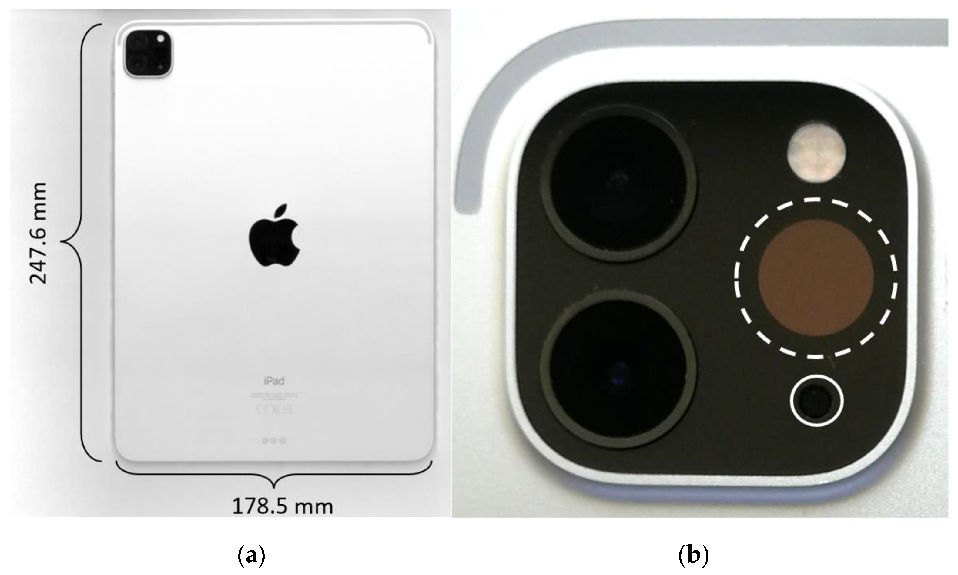
2.2. Instrumentation

A total of 21 sample plots were scanned in December 2020 using an iPad Pro 11” 256 GB (Apple Inc., Cupertino, CA, USA) [61] running with iOS 14.4.1 (see Figure 1a). The hand-held device (471 g) includes a LiDAR module on the rear camera cluster (see Figure 1b). Besides the specified range of approximately 5 m, Apple does not provide further information on the accuracy of the respective technology and hardware specifications. However, it is known from reverse engineering that the LiDAR module consists of an emitter (vertical-cavity surface-emitting laser with diffraction optics element, VCSEL DOE) and a receptor (single-photon avalanche diode array-based near infra-red complementary metal-oxide-semiconductor image sensor, SPAD NIR CMOS) based on direct-time-of-flight technology [73]. With the help of the wide (main)- and ultra-wide camera module, it is possible to produce colorized 3D models. The associated operating system (iOS 14 and advanced) provides developers access to the sensors and the built-in 3D environment mapping through ARKit [74].
In initial trials, we tested a set of 8 different scanning apps: 3D Scanner App [75], Polycam [76], SiteScape [77], LiDAR Scanner 3D [78], Heges [79], LiDAR Camera [80], 3Dim Capture [81] and Forge [82]. Out of these, the following 3 applications were judged as suitable for the actual practice tests under a forest environment:
(i)
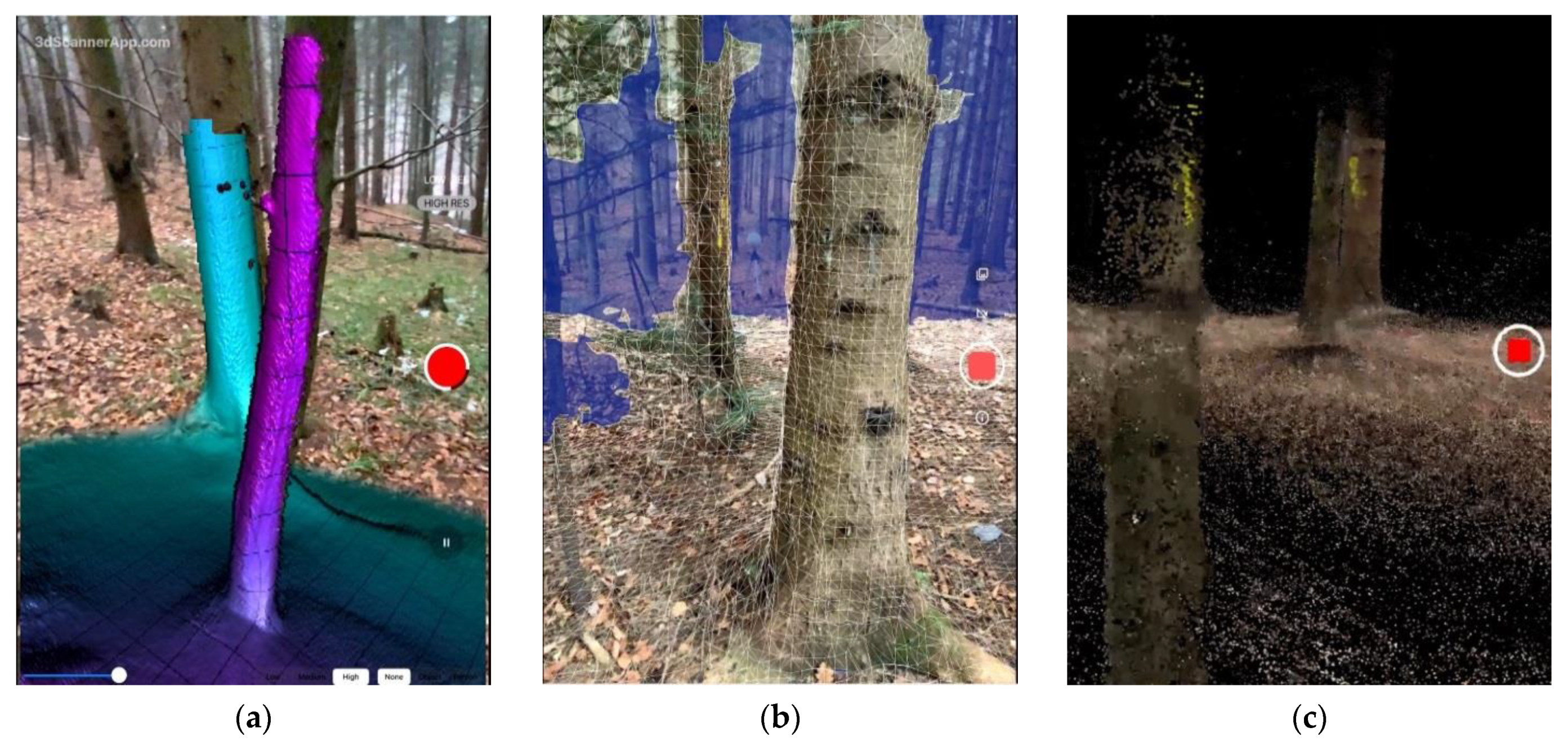
3D Scanner App 1.8.1 [75] (Laan Labs, New York, NY, USA) was used in High Res mode, with the following settings: max depth = 5 m; resolution = 10 mm; confidence = high; masking = off. The scans were colorless, and no postprocessing was required.
(ii)
Polycam 1.2.7 [76] (Polycam Inc., San Francisco, CA, USA) did not offer any setting options for the scan and was thus used in standard mode. Postprocessing of the scans was necessary and performed within the app, using the standard quality setting. As raw scan data were saved, postprocessing could be conducted any time after the completion of the scans.
(iii)
SiteScape 1.0.2 [77] (SiteScape Inc., New York, NY, USA) was used with the following settings: scan mode = max area; point density = low; point size = low. The scan was automatically post-processed in the app directly after scanning.

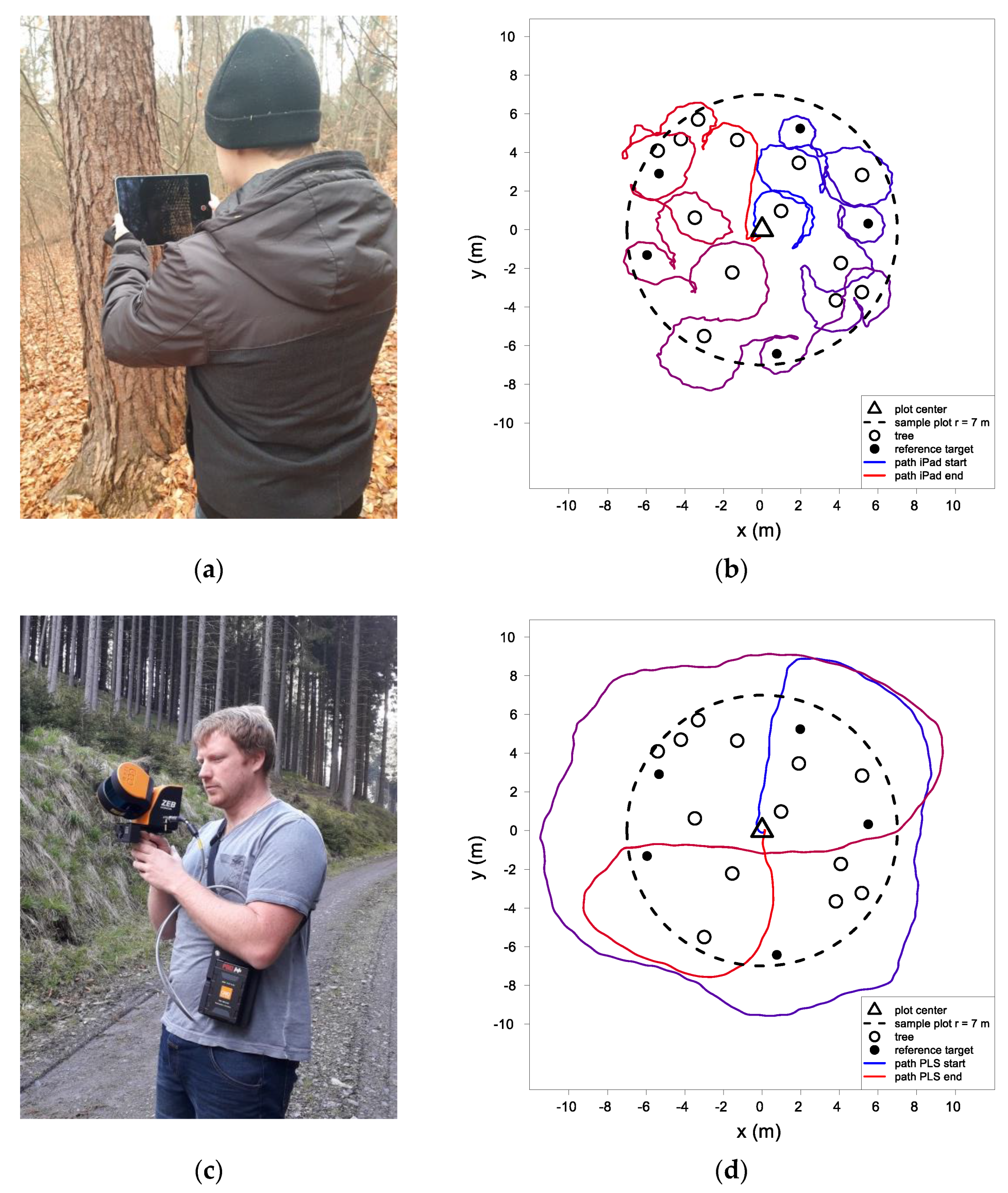
2.3. Data Collection

The data acquisition with the iPad laser scanner started at the sample plot center. After the initialization time (this was different among the tested scanning apps), the scan was performed by moving at walking speed while the LiDAR sensor collected the 3D measurement data. In preliminary tests, a proper solution was elaborated for the alignment of the walking path. As a consequence, the field worker surrounded every tree individually, and the iPad LiDAR sensor was pointed at the stems to guarantee that the 3D point cloud contained sufficient data of every single stem. The iPad was carried at a height of approximately 1.3 m, which ensured that both stems and the ground could be captured. The sample plot radius was constantly set to 7 m, plus an additional 1 m outer buffer zone. On average, the scan took approximately 5–10 min per sample plot, but the scan time slightly differed depending on the number of trees, the stand structure, terrain characteristics, and the resulting possible walking speed. The actual recording time was recorded manually by a second person. Details on how the iPad was carried across the plot as well as on the walking path can be found in Figure 2a,b. Screen shots from the iPad scans with all three apps can be found in Figure 3, and screen videos can be found in https://doi.org/10.5281/zenodo.5070671.
Extra PLS data were simultaneously collected with a GeoSLAM ZEB HORIZON (GeoSLAM Ltd., Nottingham, UK) [83] system on the same sample plots directly after the iPads scans were completed. The GeoSLAM ZEB HORIZON measures 300.000 points per second with a maximal measuring distance of 100 m and a range accuracy of ±3 cm, using time-of-flight technology. The angular field of view is 360° × 270° [83].
The walking path was carried out based on the findings of Gollob et al. [50], ensuring optimal coverage of the plot area, a low scanner range noise, and a low position accuracy drift. By starting at the plot center and walking in the north direction, the circular sample plot with a 7 m radius was surrounded once with a 2–3 m buffer zone and then crossed twice with the GeoSLAM PLS system. The scanning process ended at the plot center. A single PLS scan took approximately 3–7 min per sample plot. Details on how the PLS system was carried across the plot as well as on the walking path can be found in Figure 2c,d. For further information on the PLS scanner and the hardware parameter settings, the reader is referred to Gollob et al. [50,84].
To enable an easy co-registration of the iPad and PLS scans, five reference spheres with a 200 mm diameter were mounted on tripods and served as reference objects for the later co-registration of the 3D point clouds. On each plot, the spheres were regularly aligned in equal distances of approximately 6–7 m to the plot center.

2.4. Point Cloud Processing, Clustering, Detection of Tree Positions, and dbh Measurement

A step-by-step overview of the entire workflow and detailed parameter settings is given in Appendix A, Table A2.
When the iPad field data collection and postprocessing was completed, the scans from all three apps were exported as *.ply (Polygon File Format [85]) files to a desktop computer using iTunes [86]. PLS field data were transferred from the data logger to a desktop computer for the subsequent postprocessing with the GeoSLAM Hub 5.2.0 software [87]. The origin of each registered PLS point cloud lay at the start/end point of the walking path (local coordinate system). The PLS data for each of the 21 sample plots were exported in the LAS file format [88] using the GeoSLAM Hub settings “100% of points“, “time stamp: scan“, and “point color: none”.
For the comparison of the registered iPad and PLS point clouds, the iPad point clouds were rotated and translated to the coordinate system of the PLS data via the coordinates of the five reference spheres. First, the spheres were fit to the reverence targets in the point clouds using CloudCompare v2.10.2 [89]. With the help of the sphere’s center coordinates, the rotation and the translation were operated with CloudCompare’s align function. This step had an accuracy (RMS in CloudCompare) of 5–20 cm. The transformed iPad point clouds were exported in the LAS-file format. Examples of final point clouds from iPad and PLS can be found in Figure 4.
Further point cloud processing and analysis, including the DTM generation, the detection of tree positions, and the dbh measurement, was performed by using an algorithm presented by Gollob et al. [50] that was programmed in the statistical computing language R [90]. Henceforth, the point clouds of the scans with iPad and PLS were processed and analyzed with the same algorithms. A step-by-step overview of the algorithms and detailed parameter settings is given in Appendix A, Table A2. The diameter modeling was carried out with five different approaches, namely two regression spline models, two circle fit variants, and an ellipse fit. All diameter estimates were fitted to 15 cm wide cross-sections of the point cloud selected at 1–2.6 m (iPad: 0.2–1.8 m) height above ground. The d g a m estimate was obtained by a cyclic cubic regression spline. For the d t e g a m estimate, we used a bivariate cyclic tensor product smoother across both the vertical and the horizontal axis. The circle fit estimates d c i r c and d c i r c 2 were obtained by a circular cluster method and a least-squares-based algorithm, respectively. For the ellipse fit d e l l a direct least squares algorithm was used. A cross-section example of a single tree for the three different iPad apps and the PLS with different diameter approaches is shown in Figure 5. Differences in the individual parameters between the iPad and PLS can also be seen in Appendix A, Table A2. For further details on the algorithms, the reader is referred to Gollob et al. [50].

2.5. Evaluation of Point Cloud Quality and Diameter Fitting on Cylindrical Reference Objects

As the iPad with an integrated LiDAR sensor and the associated scanning apps were newly available on the market, the point cloud quality and the diameter estimation accuracy were also evaluated on six cylindrical objects (Figure 6). These objects were scanned under constant indoor lighting and weather conditions to assess the potential accuracy of the iPad under in vitro conditions and to exclude possible disturbance effects from the outdoor forest environment. The tests with the cylindric reference objects also eliminated other effects, which might be introduced by the different tree species or the bark structure and could produce a bias or an extra noise in the diameter estimation. Table 2 shows an overview of the different shapes, materials, and diameters of the objects. In general, the objects had a clean and even surface and consisted of plastic (objects 1, 4, and 6) and metallic (objects 2–3, 5) material. The diameters of the cylindrical objects (between 6.5 cm and 49.9 cm) were measured with a caliper. During the scanning process with the iPad and PLS, special care was taken that the objects received laser beams from all sides and that the laser beams did not hit the inner side of the hollow-shaped objects. For the latter purpose, the upper openings of the objects were covered with solid lids. The scanning process, the point cloud generation, and the processing were performed as described in Section 2.3 and Section 2.4.
In order to obtain individual object point clouds, PLS and iPad clouds were manually clipped and subsequently saved in the LAS file format [88] using CloudCompare v2.10.2 software [89]. Diameters d g a m and d c i r c 2 were fitted at the half object height using the methods described in Section 2.4. The deviation δ of the fitted diameters d ^ from the reference diameters d was calculated as follows:
δ = d ^ d .
The noise of the point clouds was assessed in terms of the standard deviation of the residuals from d g a m ( s d r e s _ g a m ). Both δ and s d r e s _ g a m were compared for each object between the iPad measures with the 3D Scanner App, Polycam, and SiteScape and with the PLS measures.

2.6. Reference Data

Reference data of the actual dbh values and tree positions were measured in a field campaign accomplished in December 2020. Based on a preliminary stem map that was produced in previous studies by Gollob et al. [14,50], the trees were recorded if their dbh (measured in direction to the plot center with calipers in 1.3 m height) was greater than or equal to a lower threshold of 5 cm and if their distance from the sample plot center was equal to or less than 8 m. New trees that had not been captured in the preliminary stem map were additionally recorded via the distances and angles to two other known tree positions. Due to possible deviations from the exact sample plot center as well as from the north direction, an affine transformation of the detected tree positions (from iPad or PLS) was carried out. The affine transformation was accomplished using the AffineTransformation() function in the R package vec2dtransf [91] with the coordinates of 10–15 trees per sample plot that were found by the algorithm (iPad and PLS trees) and that were also present in the reference data. The final alignment of the tree positions from the iPad and PLS scans to the reference coordinates was performed using the function pppdist() in the R package spatstat [92].

2.7. Accuracy of Tree Detection, dbh Measurement, and DTM

The accuracy of tree detection was calculated in terms of the following measures: detection rate d r ( % ) , commission error c ( % ) , and overall accuracy a c c ( % ) . These measures were calculated as follows:
d r ( % ) = n match n ref × 100 ,
c ( % ) = n falsepos n extr × 100 ,
a c c ( % ) = 100 % ( o ( % ) + c ( % ) ) ,
where n match is the number of correctly found reference trees, n ref is the total number of reference trees, n falsepos is the number of tree positions that could not be assigned to an existing tree in the reference data, n extr is the number of automatically detected tree positions ( n match + n falsepos ) and o ( % ) is the omission error defined as 100 % d r ( % ) . The detection rate d r   ( % ) measures the proportion of correctly detected tree locations, the commission error c   ( % ) measures the proportion of falsely detected tree locations, and the overall accuracy a c c ( % ) is a combination of the latter two metrics and represents a global quality criterion.
The accuracy and precision of the DTM and the dbh measurements were assessed by means of the root mean square error (RMSE) and the bias. For the tree positions, only the RMSE was calculated. RMSE and bias were calculated based on the deviation between the automatic measurement y ^ i and the corresponding reference measurement y i :
RMSE = 1 n match i = 1 n match ( y ^ i y i ) 2 .
bias = 1 n match i = 1 n match ( y ^ i y i ) .
The deviation between the automatic dbh measurement d b h ^ i and the corresponding reference measurement d b h i was computed analogously to Equation (1) and is termed δ d b h .
RMSE and bias were also calculated as relative measures (RMSE% and bias%):
RMSE % = RMSE y ¯ × 100 ,
bias % = bias y ¯ × 100 ,
with
y ¯ = 1 n match i = 1 n match y i
being the average of the reference data. Hereof, n match is the number of matched pairs from the extracted values to reference values. When the accuracy of the DTMs was analyzed, the elevation values of the raster cells from the PLS DTM served as reference values. To evaluate the tree position, the distances from each tree to its neighbors were calculated and compared with the reference distances from the PLS scans. This was only performed for those trees that were correctly found in all four scans (three iPad and PLS scans). To examine whether the performance of the iPad and PLS scans and the automatic routines showed tree size-dependent trends, the performance measures were separately evaluated for three different lower dbh thresholds of 5 cm, 10 cm, and 15 cm.

3. Results

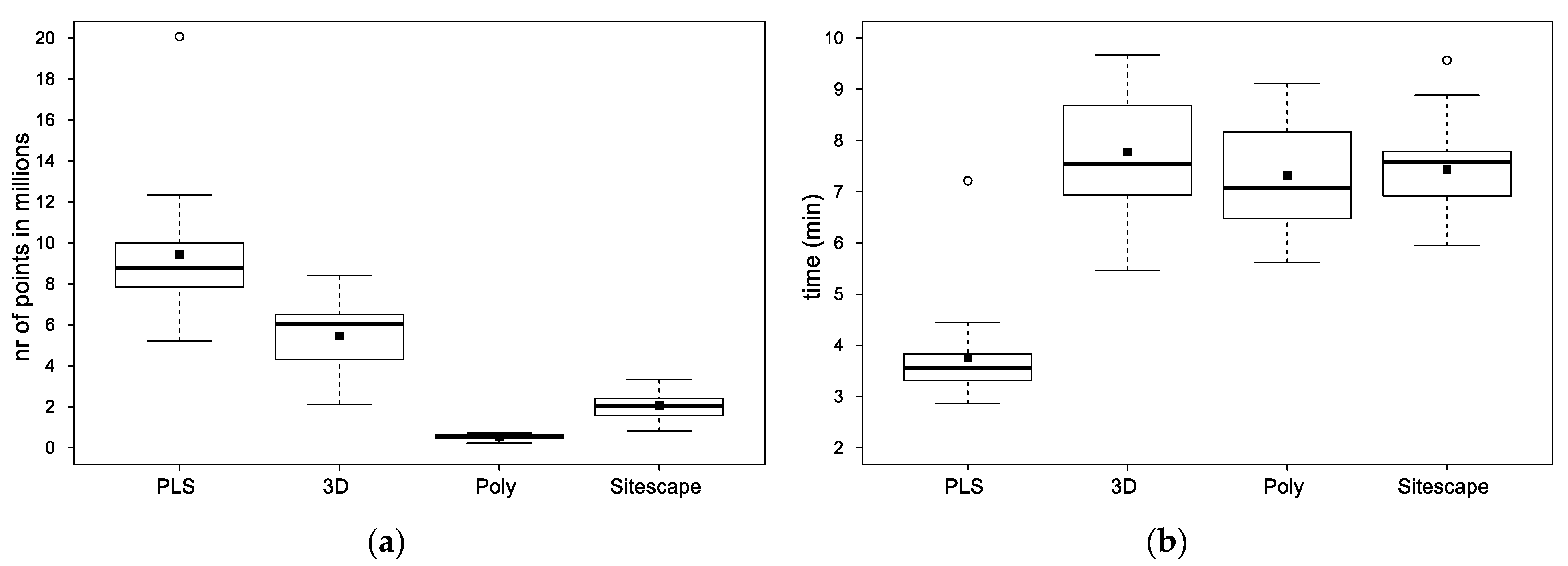
3.1. Acquisition Time and Number of Points

With the PLS, the acquisition time for the 21 sample plots (r = 7 m) ranged from 2.9 min to 7.2 min, and 5.2–20.1 million 3D points were collected per plot (Figure 7). The respective average values were 3.8 min and 9.4 million points, resulting in an average acquisition rate of 41,228 points per second. Thus, a large proportion of the 300,000 points per second sampled by the PLS fell outside of the sample plots. In general, the iPad scans (3D Scanner App, Polycam, and SiteScape) were produced in a higher acquisition time and had a lower number of 3D points. With the 3D Scanner App, the acquisition time ranged from 5.5 min to 9.7 min (average 7.8 min) and produced 2.1–8.4 million points (average 5.4). Polycam was able to capture between 0.2 and 0.7 million 3D points (average 0.5) within 5.6 min–9.1 min (average 7.3 min). The acquisition time for SiteScape ranged from 6.0 min to 9.6 min (average 7.4 min) and produced 0.8–3.3 million 3D points (average 2.1). The acquisition rate in points per second with the 3D Scanner App, Polycam, and SiteScape was 11,538, 1141, and 4730, respectively. Further details on the acquisition time and the cardinality of the point clouds per sample plot can be found in Appendix B, Table A5.

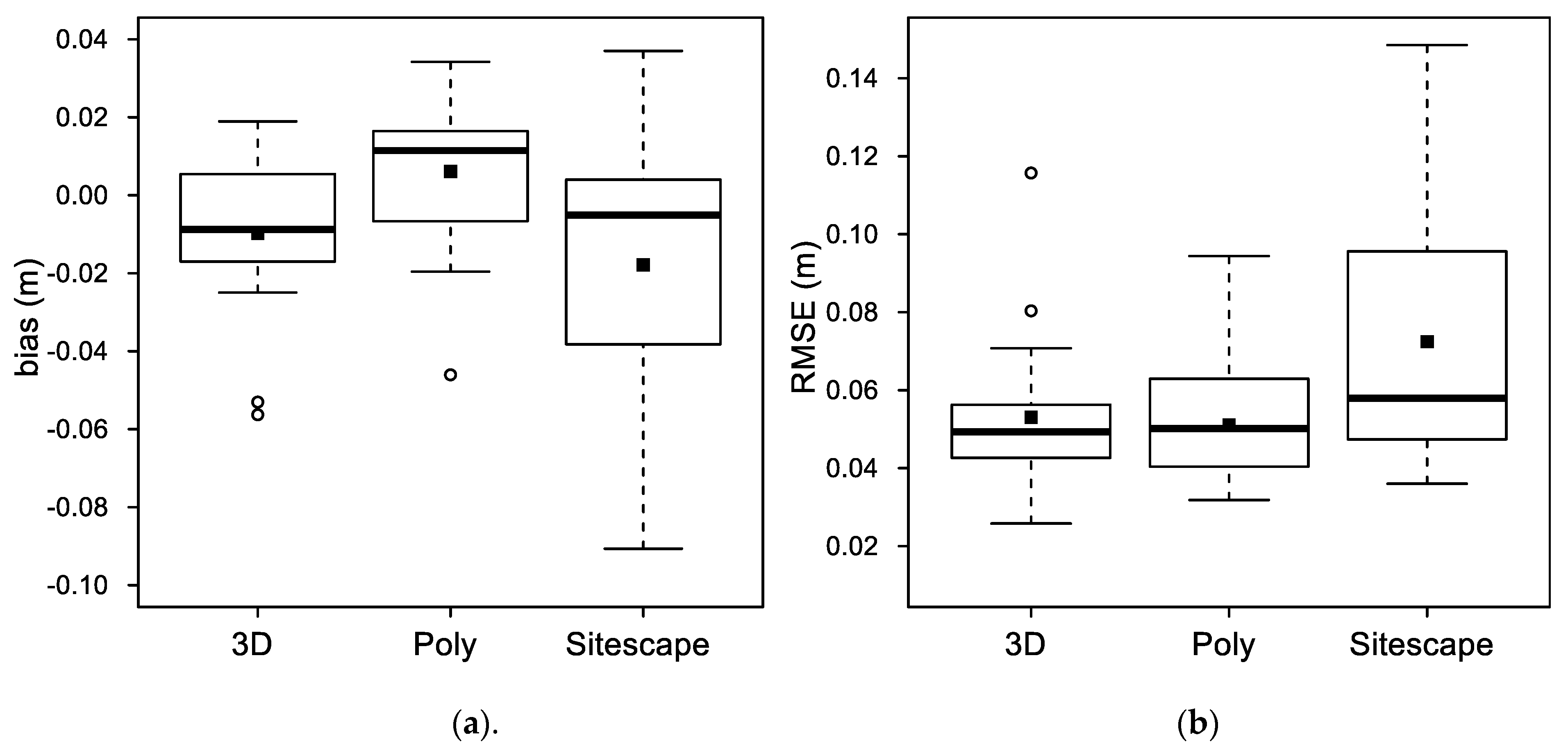
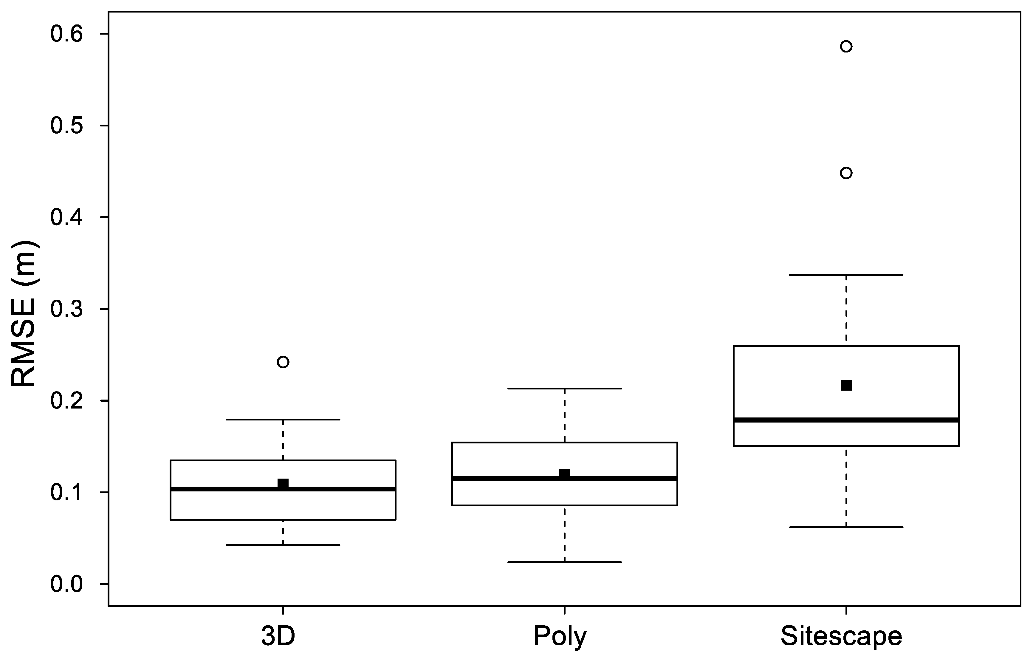
3.2. Digital Terrain Model (DTM)

The performance of the DTM models was assessed in terms of the deviation between the iPad DTM height estimates and the PLS DTM (Figure 8). The reference DTMs from the PLS data always provided full coverage of the entire sample plot area (coverage = 100%). In contrast, the iPad DTMs had empty cells, i.e., data were missing for some of the grid cells due to incomplete scans. The corresponding average coverage rates of the 3D Scanner App, Polycam, and SiteScape were 98.8%, 99.4%, and 99.6%, respectively. Missing values were not interpolated for the iPad DTMs, and only the available-data grid cells were considered for the evaluation of the DTMs. Evaluations of the DTMs from the 3D Scanner App showed an RMSE of 0.026–0.116 m (average: 0.053 m) and a bias of −0.056–0.019 m (average: −0.010 m). The Polycam DTMs had an RMSE of 0.032–0.094 m (average: 0.051 m) and a bias of −0.046–0.034 m (average: 0.006 m). The RMSE of the SiteScape DTMs was 0.036–0.149 m (average: 0.072 m), and the bias was −0.091–0.037 m (average: −0.018 m).

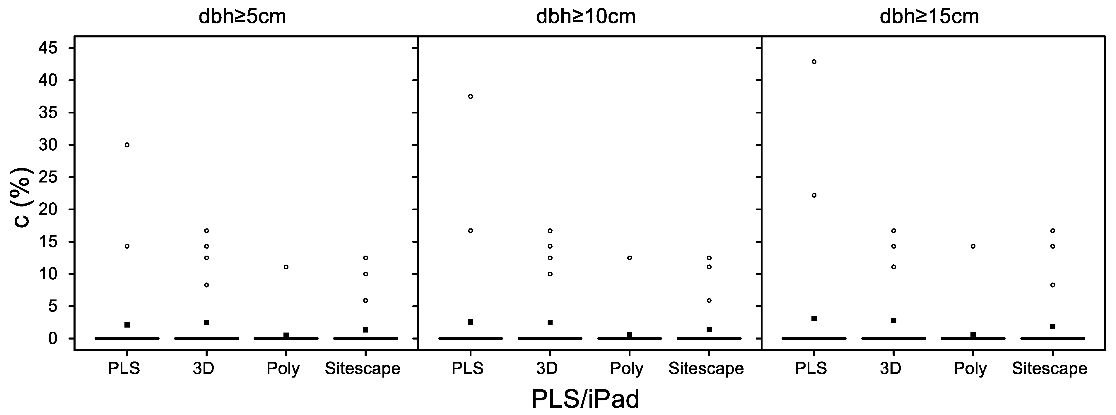
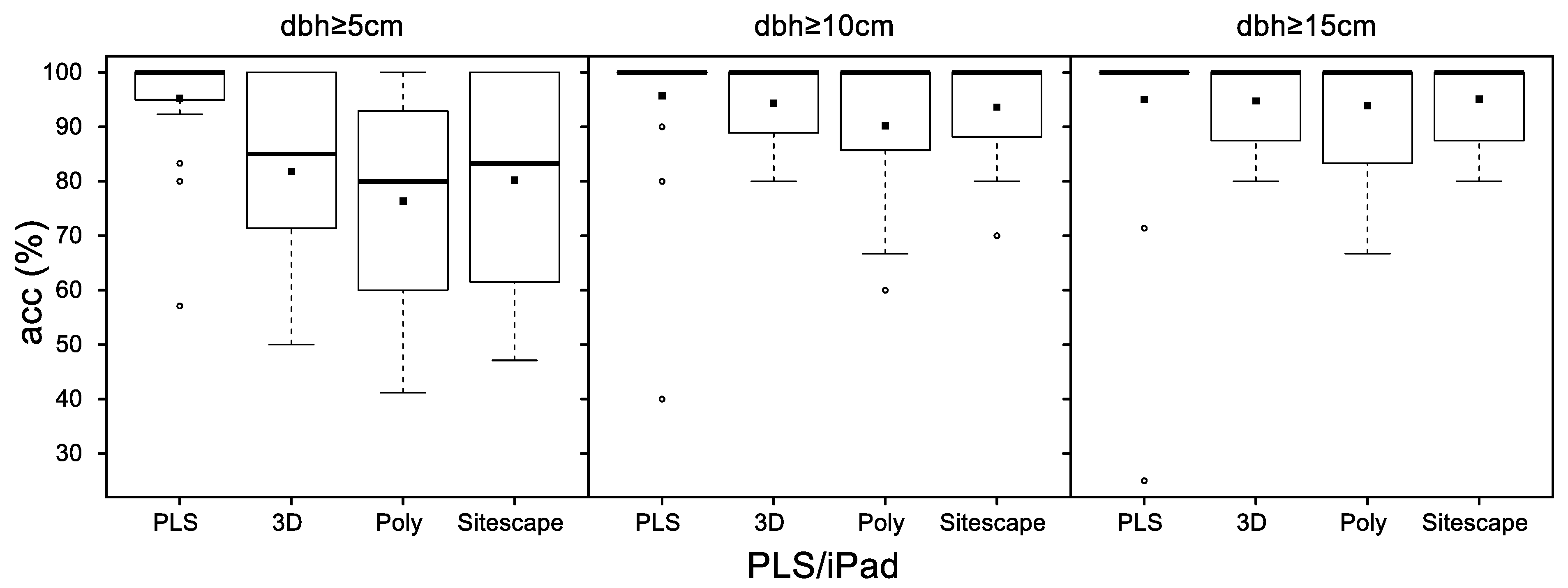
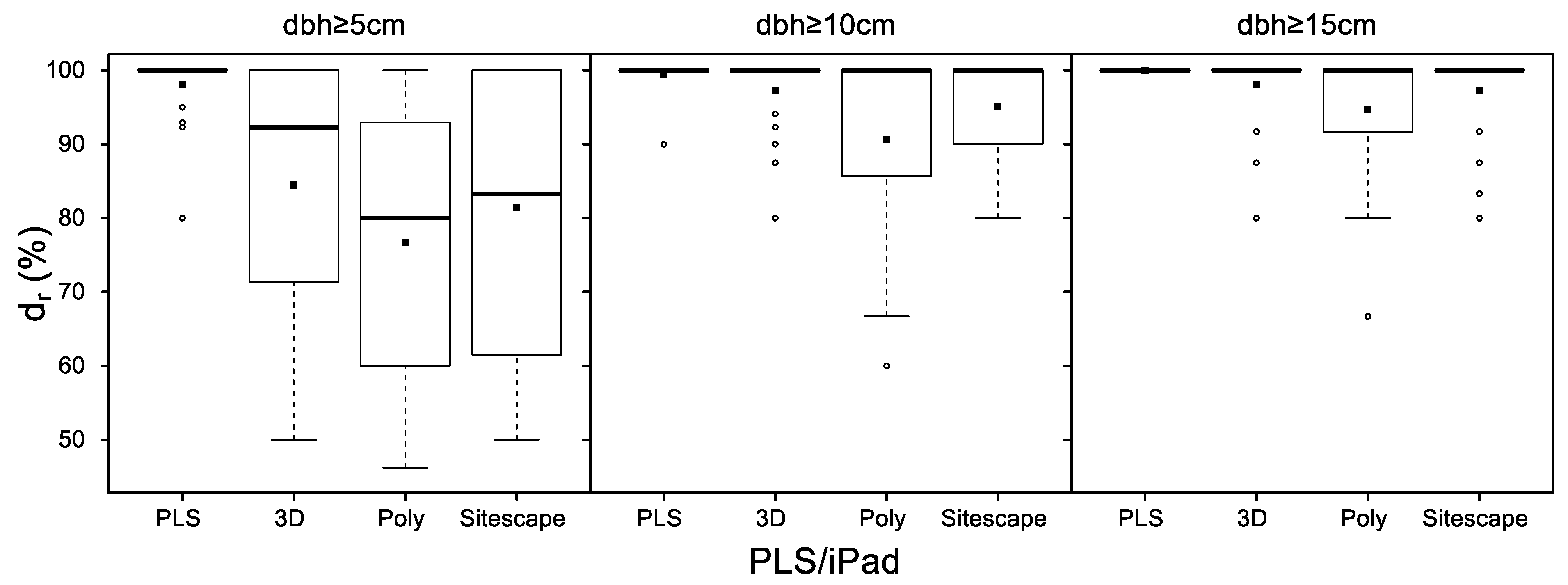
3.3. Detection of Tree Positions

The analysis of the 21 sample plots showed that the tree detection rate d r ( % ) was strongly dependent on the lower dbh threshold (Figure 9). In general, the detection rate showed an increasing trend with an increasing dbh threshold. Furthermore, the iPad scans (3D Scanner App, Polycam, and SiteScape) generally produced lower detection rates than the PLS scans, especially when a lower dbh threshold was considered. A steep increase in the detection rate with the iPad data was found for a lower dbh threshold between 5 cm and 10 cm. The range of possible detection rates with PLS was always smaller than with the iPad. The average detection rates over all 21 sample plots and dbh thresholds were 84.49–98.06% with the 3D Scanner App, 76.67–94.68% with Polycam, and 81.41–97.26% with SiteScape. The corresponding average detection rates with PLS ranged from 98.10% to 100%. Using a lower dbh threshold of 10 cm, the respective average detection rates with the 3D Scanner App, Polycam, SiteScape, and PLS were 97.33%, 90.65%, 95.06%, and 99.52%, respectively. For further details on the average detection rates, the reader is referred to Appendix B, Table A3, and for details on individual sample plot results, to Table A5. Using a lower dbh threshold of 10 cm, a detection rate of 100% was achieved on 76%, 52%, and 67% of the sample plots using 3D Scanner App, Polycam, and SiteScape, respectively. Using PLS, a detection rate of 100% with a lower dbh threshold of 10 cm was achieved on 95% of the sample plots; i.e., on all but one plot, all the existing tree positions were automatically detected. The average detection rate over all sample plots and for a 10 cm dbh threshold was 96.97%, 90.30%, 94.55%, and 99.40% with the 3D Scanner App, Polycam, SiteScape, and PLS, respectively.
The commission error   c ( % ) showed a slightly increasing trend with an increasing lower dbh threshold (Figure 10). In general, the average commission error and its range were smaller with all iPad apps than with PLS. Over all 21 sample plots and dbh thresholds, the average commission error was 2.47–2.80% with the 3D Scanner App, 0.53–0.68% with Polycam, and 1.35–1.87% with SiteScape. The corresponding average commission error with PLS was 2.11–3.10%. For further details on the average commission errors, the reader is referred to Appendix B, Table A3, and for details on the per-sample plot results, to Table A5. The overall commission errors, i.e., regardless of the individual sample plots, with a lower dbh threshold of 10 cm, were 2.44%, 0.67%, 1.89%, and 2.96% for the 3D Scanner App, Polycam, SiteScape, and PLS, respectively.
The overall accuracy rates a c c ( % )   as a joint quality criterion of the detection and commission rates, are presented in Figure 11. The overall accuracy showed similar trends as the detection rates dependent on a changing lower dbh threshold. The average overall accuracy across all 21 sample plots and dbh thresholds was 81.80–94.76% with the 3D Scanner App, 76.39–93.89 with Polycam, and 80.21–95.11% with SiteScape. The average overall accuracy with PLS varied between 95.07% and 95.27%. Using a lower dbh threshold of 10 cm, the average overall accuracies with the 3D Scanner App, Polycam, SiteScape, and PLS were 94.37%, 90.18%, 93.62%, and 95.71%, respectively. For further details on average overall accuracies, the reader is referred to Appendix B, Table A3, and for the details per sample plot, to Table A5. The overall accuracies with a lower dbh threshold of 10 cm, regardless of the individual sample plots, were 94.53%, 89.63%, 92.66%, and 96.36% for the 3D Scanner App, Polycam, SiteScape, and PLS, respectively.

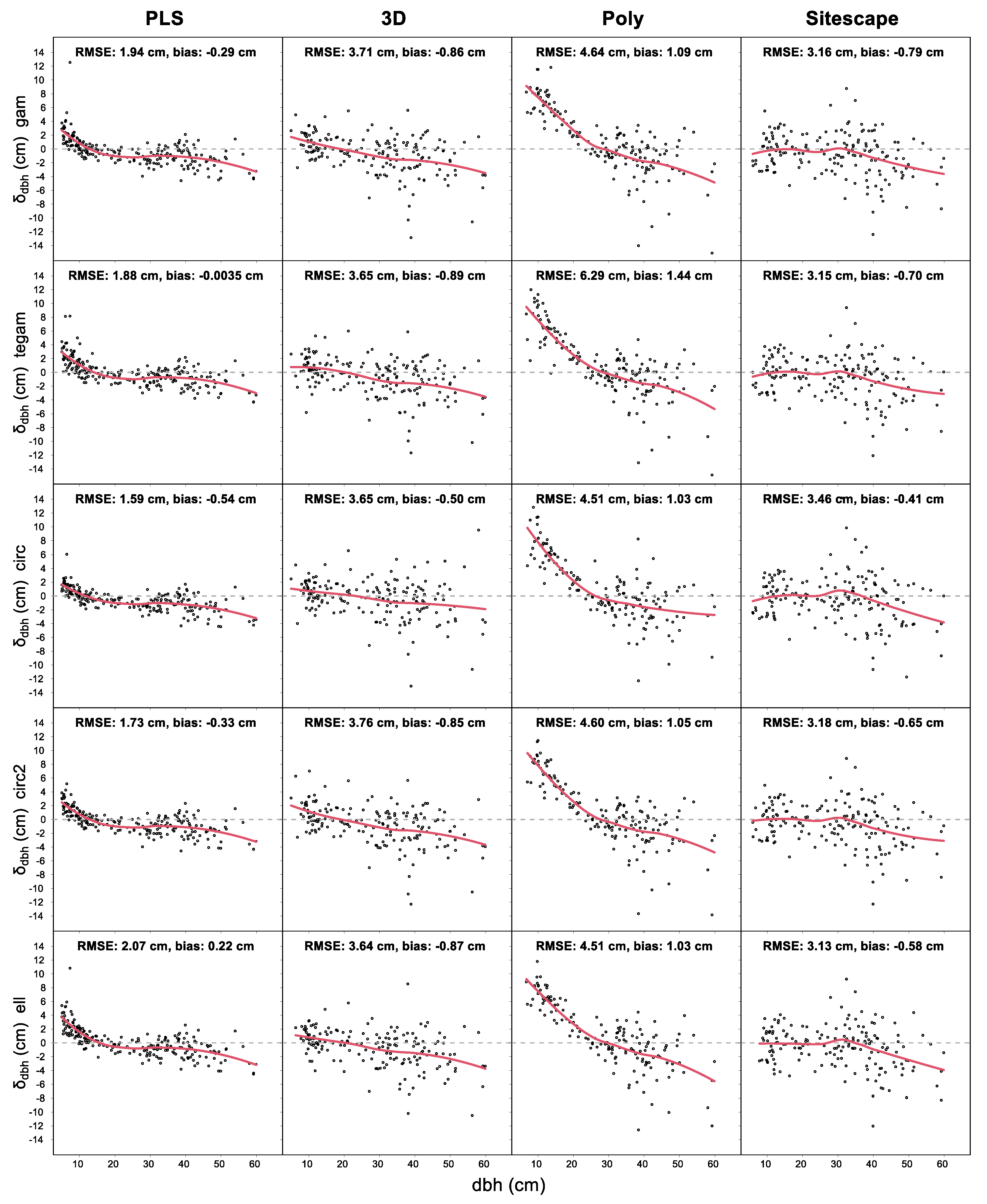
3.4. Estimation of dbh

The performance of the automatic dbh estimation, in terms of the deviation of the iPad and PLS dbh estimates from the field measurements, is shown in Figure 12. All dbh fitting methods (i.e., d g a m , d t e g a m , d c i r c , d c i r c , d c i r c 2 and d e l l ) showed similar trends in the dbh deviation, but differences existed among the various iPad apps and the PLS. With the 3D Scanner App and the PLS, the smaller diameters (dbh < 15 cm) were generally overestimated, while large diameters (dbh > 15 cm) were generally underestimated. With the Polycam data, trees with diameters less than 25 cm were generally overestimated, and trees with diameters greater than 25 cm were generally underestimated. SiteScape did not show a bias for a dbh less than approximately 30 cm, but underestimations were produced for a larger dbh. In sum, the underestimation increased with further increasing dbh, and the overestimation increased with decreasing dbh. When the various dbh fitting methods were further analyzed, the RMSE with the 3D Scanner App was 3.64–3.76 cm (12.65–13.21%), and the bias was −0.89–−0.50 cm (−3.13–−1.75%). The lowest RMSE was obtained by d e l l (3.64 cm = 12.65%), while the lowest bias was obtained by d c i r c (−0.50 cm = −1.75%). With Polycam, the RMSE of the dbh fitting methods was 4.51–6.29 cm (15.11–21.23%), and the bias was 1.03–1.44 cm (3.45–4.87%). The lowest RMSE (4.51 cm = 15.11%) and the lowest bias (1.03 cm = 3.45%) were obtained by d c i r c and d e l l . The RMSE of the various dbh fitting methods with SiteScape was 3.13–3.46 cm (10.50–11.81%), and the bias was −0.79–−0.41 cm (−2.71–−1.38%). The lowest RMSE was obtained by d e l l (3.13 cm = 10.50%), while the lowest bias was obtained by d c i r c (−0.41 cm = −1.38%). With the PLS scans, the RMSE of the dbh fitting methods was 1.59–2.07 cm (6.29–8.29%), and the bias was −0.54–0.22 cm (−2.16–0.89%). The lowest RMSE was obtained by d c i r c (1.59 cm = 6.29%), while the lowest bias was obtained by d t e g a m (−0.004 cm = −0.01%). For further details on average detection rates, the reader is referred to Appendix B, Table A4. Performance results of the dbh ( d e l l ,   d c i r c ) estimation per sample plot are presented in Appendix B, Table A5.

3.5. Tree Location

The accuracy of the tree location (Figure 13) was evaluated by means of the distances from each tree to its neighbors. Corresponding distances derived from the PLS scans served as reference data. The RMSE of the position finding with the 3D Scanner App was 0.042–0.242 m (average: 0.109 m), with Polycam was 0.024–0.213 m (average: 0.119 m), and with SiteScape was 0.062–0.586 m (average: 0.218 m). Individual sample plot results can also be found in Appendix B, Table A5.

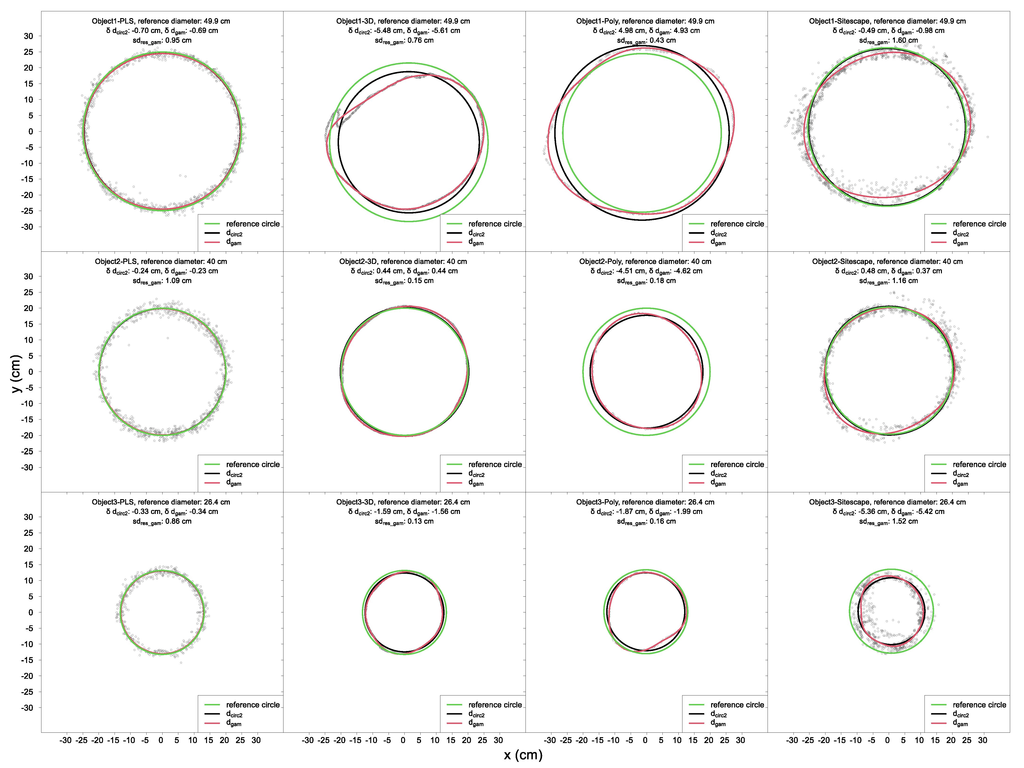
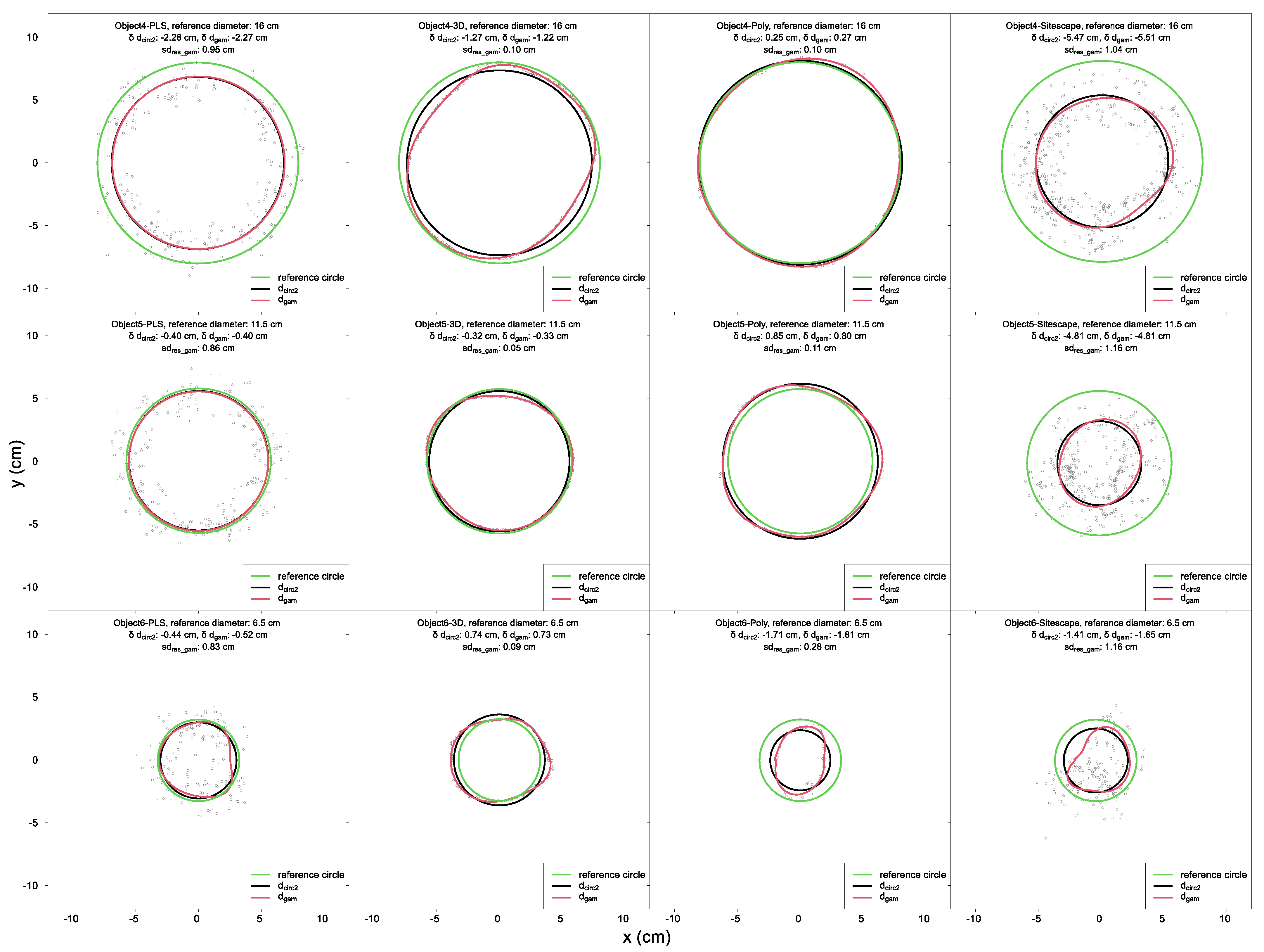
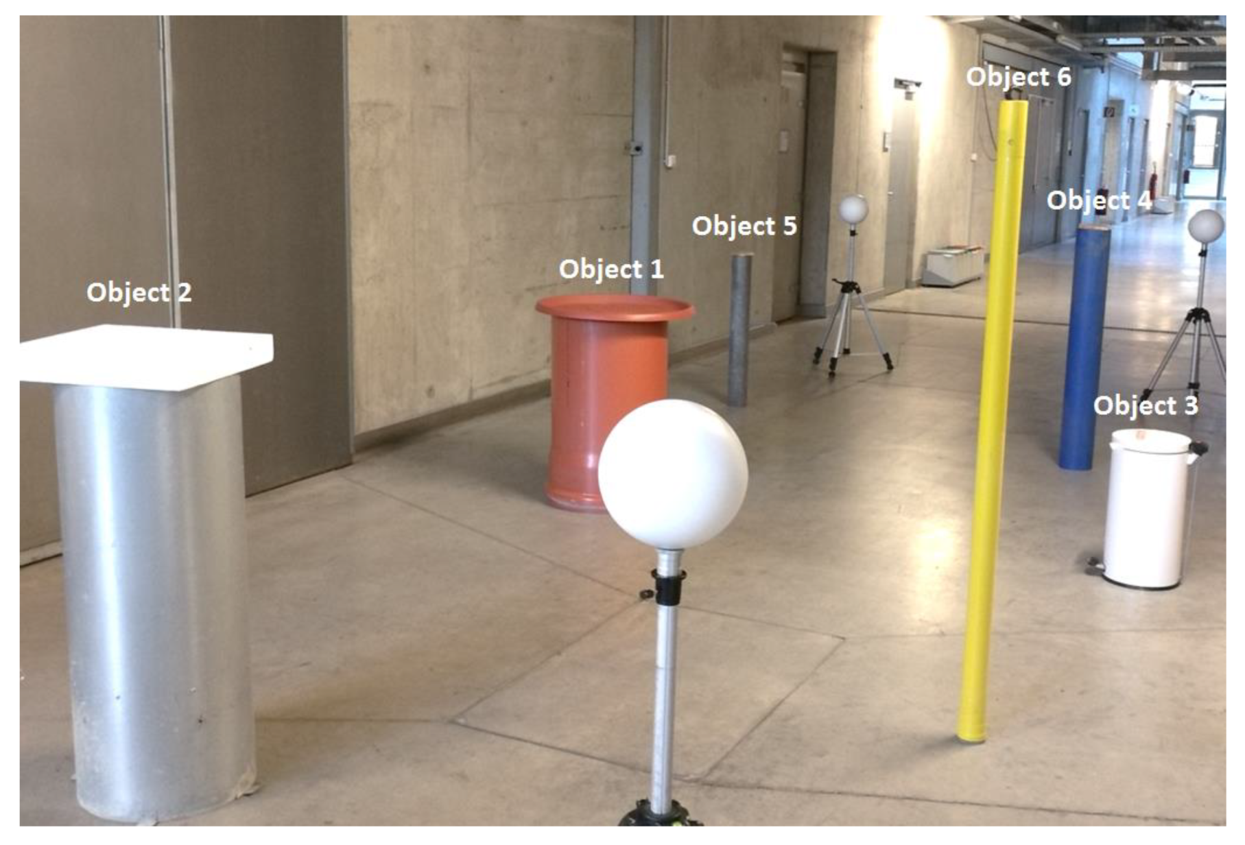
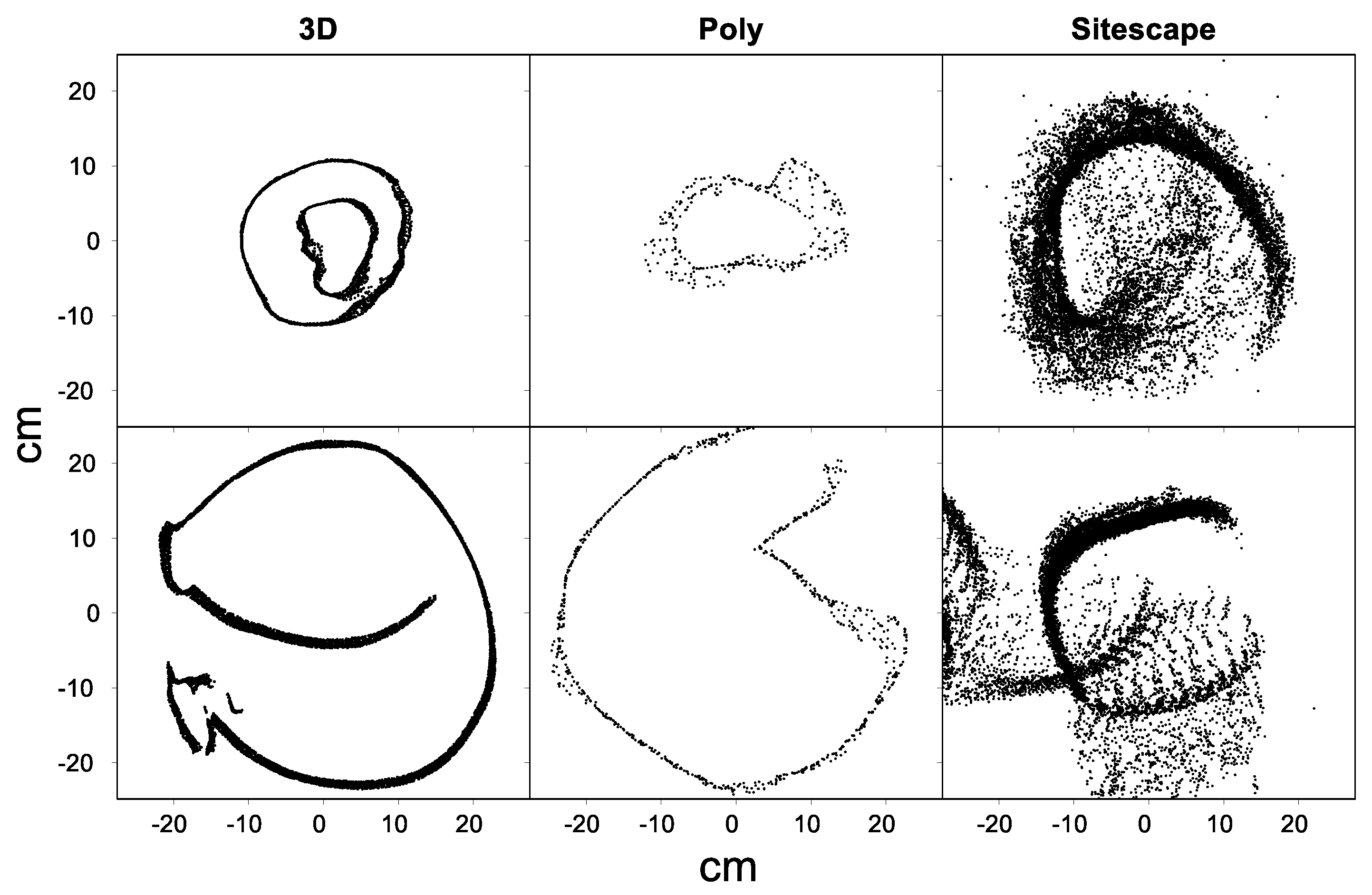
3.6. Cylindrical Reference Objects under In Vitro Conditions

The performance of the diameter measurement with the iPad scans and the quality of the iPad 3D point cloud data were further examined under in vitro conditions by means of the scans of six cylindrical objects. For the individual object point clouds from the iPad scanner apps and the PLS, the diameters d g a m and d c i r c 2 were calculated using the same algorithms as under in situ conditions in the forest. The mean standard deviation ( s d r e s _ g a m ) of the d g a m residuals was used as a measure for the noise of the point clouds. The evaluation of the three iPad scans and the PLS scan by means of the diameter deviation δ and the standard deviation of the residuals from the natural cubic spline s d r e s _ g a m   can be found in Table 3. In general, the deviations from the reference diameter were higher with the iPad than with PLS. Furthermore, the standard deviation of the residuals s d r e s _ g a m (noise in the point cloud) was relatively low with the 3D Scanner App (0.05–0.76 cm) and with Polycam (0.10–0.43 cm). s d r e s _ g a m was 1.04–1.60 cm with SiteScape and 0.83–1.09 cm with PLS. The deviations did not show a trend over changing reference diameters. The highest PLS diameter deviation occurred on object 4 (−2.28 cm). With the 3D Scanner App, object 1 had the highest deviation (−5.61 cm) in terms of the s d r e s _ g a m noise parameter. The PLS scans showed a systematic underestimation (−0.23 to −2.28 cm) of the diameters, while the three iPad apps produced both underestimations and overestimations (−5.61 cm to 4.98 cm). A comparison of the diameter fitting methods ( d g a m and d c i r c 2 ) showed that with the iPad and PLS, basically, a trend did not exist for lower or higher deviations. An overview of the six object cross-sections, including the fitted diameters, deviations, and standard deviations of the residuals, can be found in Appendix C, Figure A1 and Figure A2.

4. Discussion

4.1. DTM Modelling, Stem Detection and DBH Estimation

In this study, existing algorithms were used that were formerly developed by Gollob et al. [50]. All routines worked fully automatically with the scan data from the three iPad apps and with the PLS scans. Data acquisition with the iPad and the PLS was accomplished on the same days on all sample plots. That is, the different scanning methods (iPad and PLS) were tested under nearly constant environmental conditions and by means of the same reference data. However, the pre-processing of the LiDAR raw data was accomplished with different software programs; the PLS data were pre-processed with GeoSLAM Hub and the iPad data with the respective apps. The subsequent point cloud processing and analysis were performed with the statistical software R (R Foundation for Statistical Computing, Vienna, Austria) [90] and by using the CloudCompare software [89]. Hence, most of the workflow was carried out with freely available and programmable software. For each sample plot and scanner system (iPad and PLS), constant parameter settings were applied for the DTM models, for the cluster algorithms of tree position finding, and for the diameter estimation programs. Very few changes were necessary (see Appendix A, Table A2) in order to consider inherent differences in the completeness and quality of the point clouds between the iPad and the PLS. Nevertheless, the settings were held fixed among the three iPad apps (3D Scanner App, Polycam, and SiteScape) throughout.
The performance of the DTM modeling with the point clouds from the three iPad apps was evaluated by means of the PLS reference terrain model. Alternatively, the reference DTM could have also been measured in situ, e.g., by using a total station. However, this would have caused overly high labor costs. Besides, the DTMs that were automatically produced from the point clouds had a 20 cm pixel resolution. Hence, it was hardly possible to obtain such a high resolution using a traditional total station. In conclusion, it was assumed that the PLS delivers the most accurate DTM with the currently available technologies. The lowest RMSE from the PLS DTM was achieved with Polycam (5.1 cm), but the RMSE with the 3D Scanner App was only slightly higher (RMSE: 5.3 cm). The SiteScape app produced the highest RMSE with 7.2 cm. In addition to the RMSE, the percentage of the DTM covered by iPad apps was also considered by the evaluation since the combination of the RMSE and the coverage gives a fairer evaluation than the single RMSE parameter. The coverages for 3D Scanner App, Polycam, and SiteScape were 98.8%, 99.4%, and 99.6%, respectively, which showed that the apps captured almost the complete terrain of the sample plots.
Using the PLS scans resulted in better tree detection rates than with the scans of the iPad apps. Nonetheless, all three iPad apps were able to achieve detection rates greater than 90% for trees with a lower dbh threshold of 10 cm. Compared to traditional measurement techniques, the acquisition time with the iPad was 2.5 times faster. Compared to PLS, the iPad measurements were only twice as slow. Among the iPad apps, the 3D Scanner App achieved the highest detection rates. Using the 3D Scanner App and a dbh threshold of 10 cm, the detection rate was 97.33% (sd ± 5.48%) given an acquisition time of 7.77 min (sd ± 1.16 min). The detection rates of Polycam (90.65%, sd ± 12.46%) and SiteScape (94.68%, sd ± 7.83%) were significantly lower, and the increase in the acquisition time was not much higher, with 7.32 min (sd ± 1.06 min) and 7.44 min (±0.87 min), respectively.
For the three iPad apps, larger differences were found in the detection rates over a changing lower threshold dbh, especially for threshold diameters between 5 cm and 10 cm. This could be explained by the fact that the apps often failed in the mapping of thin objects. This problem was particularly evident when several objects were scanned in one scanning path, as this usually occurred on sample plots with a high stem density of smaller trees. With PLS and by using a lower dbh threshold of 10 cm, a detection rate of 99.52% (sd ±2.18%) was achieved. The corresponding acquisition time was 3.76 min (sd ±0.89 min). The proportion of falsely detected trees (commission error) was 2.55% (sd ±5.49%) with the 3D Scanner App, 0.60% (sd ±2.73%) with Polycam, 1.40% (sd ±3.69%) with SiteScape, and 2.58% (sd ±8.79%) with the PLS. Although the average commission error was relatively low, outliers were produced in very few cases with higher commission errors of approximately 10% across all iPad apps and the PLS. This was especially due to the occasionally small absolute number of reference trees on the relatively small sample plot area.
An accurate tree position finding is necessary to determine whether a tree is located on a particular plot and whether it is included by the sampling scheme. The accuracy of the tree position finding was evaluated by means of the distances from each tree to its neighbors using the corresponding distances from PLS as reference data. The 3D Scanner App had the highest accuracy in terms of the RMSE with 10.9 cm. Whereas, Polycam performed only slightly worse (RMSE: 11.9 cm), SiteScape produced the highest RMSE of 21.8 cm. An advantage of using this evaluation of the tree location accuracy via the tree neighbors is that possible inaccuracies in the rotation and translation of iPad and PLS point clouds in CloudCompare were eliminated.
It was generally found that small diameters were overestimated and that large diameters were rather underestimated with both the iPad and the PLS, irrespective of the fitting method. In fact, Gollob et al. [50] found that these systematic errors were actually introduced by the novel portable laser scanner technology, as an unbiased dbh estimation of the same trees with the same algorithms was possible using TLS data. The dbh threshold at which the positive bias turns into a negative was different among the iPad apps and the PLS. Whereas this threshold was located around 15 cm for the 3D Scanner App and for the PLS, it was around 25 cm for the Polycam app. Interestingly, the overestimation trend with Polycam was several times higher than with the other apps, and it was almost linearly dependent on dbh. However, SiteScape did not produce a bias for diameters less than approximately 30 cm.
It was found that the dbh estimates modeled with ellipses ( d e l l ) had the highest accuracy (RMSE: 3.64 cm, 4.51 cm, and 3.13 cm) with the iPad data from the 3D Scanner App, Polycam, and SiteScape. With PLS data, the highest accuracy (RMSE: 1.59 cm) was obtained by the circle fits ( d c i r c ). In general, the accuracy of the dbh estimation with PLS data was at least doubled compared to the three iPad apps. An interpretation of the overall bias is meaningless due to the trend of the bias over diameter.
The possible reason for the diameter overestimation of small trees with PLS was very likely the higher relative noise of the point clouds for smaller object sizes. In close conformance, it was also shown in Gollob et al. [50] that the overestimation increased with increasing noise, the latter measured by the standard deviation of the residuals from the dbh fit with natural cubic splines ( d g a m ). In fact, the three iPad apps did not produce a remarkably high noise, except the SiteScape app. This means that the reason for the overestimation and underestimation of iPad apps might be different from a possible high noise.
In ideal circumstances, the quality of the automatic algorithms used for the point cloud processing, DTM modeling, tree position finding, and dbh estimation is not affected by seasonal effects. In fact, shading effects can reduce the completeness of the point cloud during the vegetation period (i.e., in foliated stand conditions), in comparison to the situation in winter (i.e., in the defoliated stage), when our data were collected. In deciduous forests, a high stem density and lower branches, a multi-layered stand structure, or a dense understory of smaller trees could have more easily produced co-registration problems for the SLAM algorithms during the vegetation period. However, to more precisely quantify the possible seasonal effects, further research is required.

4.2. Point Cloud Quality and Field Experience

One of the major advantages of applied mobile and personal laser-scanning systems (iPad Pro [61] and PLS: GeoSLAM ZEB HORIZON [83]) is their rapid data acquisition time over the entire forest plot. Thus far, the high investment costs of TLS and PLS systems have hindered their wider application in the ground-based forest inventory practice. The PLS (GeoSLAM ZEB HORIZON) used in this study costs around EUR 50,000. Apple has recently integrated the LiDAR technology into the latest iPad Pro and iPhone 12. The price of such a consumer-level device is only around EUR 1000, providing broader community access to LiDAR technology. Although only the newest Apple devices were equipped with LiDAR sensors, and although app developers have only limited access to the sensor control, several useful apps have already been released for the 3D laser scanning with the iPad.
Initial trials with a broad collection of scanning apps (3D Scanner App [75], Polycam [76], SiteScape [77], LiDAR Scanner 3D [78], Heges [79], LiDAR Camera [80], 3Dim Capture [81], and Forge [82]) developed for Apple LiDAR showed that only the 3D Scanner App, Polycam, and SiteScape were well suited for practice applications on forest inventory sample plots. Further tests with the other apps (LiDAR Scanner 3D, Heges, LiDAR Camera, 3Dim Capture, and Forge) were stopped due to problems during the registration phase, frequent software crashes, or because the quality of the resulting point cloud was simply too weak. Out of the three abovementioned apps, the 3D Scanner App and SiteScape were cost-free, and the license price of Polycam’s pro version was only EUR 5 per month. Using the pro version was mandatory for using the data export function.
Initial tests showed that a sample plot size of 7 m radius was favorable. The point cloud data were incomplete when we used larger plot sizes, especially when the density of small trees was high. As a consequence, larger plot sizes mostly resulted in unacceptably low detection rates. Hence, the 7 m radius was subsequently used with all three iPad scanning apps.
For the scan data collected with the three iPad apps and the PLS, the registration of the points worked successfully on all sample plots. According to our field experience, the best operational procedure for scanning with the iPad was when two persons were involved during the scanning. One person was focused on the scanning while walking, while the second person stood outside the plot and supervised the trajectory and recognized the scanned/missed trees. Working in a two-person team was especially helpful in dense forest stands and when orientation was difficult as the on-the-fly visualization of the point cloud on the iPad screen did not perform well in such dense forests. In this regard, the 3D Scanner App and Polycam provide an extra useful feature in that the user can watch the background scenery via real-time imaging through the iPad camera. With SiteScape, the screen remains black; this made orientation difficult as the person had to check the screen and the environment simultaneously (Figure 3). In general, the iPad’s on-the-fly visualization of the point cloud is actually an effective pro compared to PLS with GeoSLAM; it makes flexible changes of the walking path possible.
Trials with different routes revealed that only the walking path with a surrounding scan of nearly every tree was feasible to achieve a complete point cloud of the trees on a sample plot. However, we also found that revisiting trees to obtain multiple scans per tree is actually not recommended as this easily produces misalignments. Some examples of such misalignments from revisiting scans of single trees are shown in Figure 14. In contrast to the scanning with the iPad, the scanning with the PLS is more time-efficient. The best operational procedure with PLS was that the sample plot area is first surrounded and then crossed.
In the common approach of scanning with the GeoSLAM PLS system, the scanner is exactly positioned at the same position for both the start point and the endpoint of the walking path. This mitigates registration problems and reduces noise in the point cloud. However, such an approach is not necessary for scanning with the iPad. Although the recorded iPad scan paths were less smooth and showed more zig-zagged moves than those of the GeoSLAM PLS, we could not find any differences in the quality of the point clouds from both devices. Furthermore, we could not find any differences in the quality of the point clouds when we compared the scans that were produced by a “closed” walking path (start point equals endpoint) against those obtained from an “open” walking path (start point is different from endpoint).
The energy consumption of the iPad LiDAR technology was considerably high. Although our iPad was shipped with a high-capacity 28.7 Wh battery, the battery was discharged in 2–3 h through the activated LiDAR sensor. We circumvented the problem of the high energy consumption by connecting the iPad to a power bank during travel times and longer breaks.
We found that the point clouds of the PLS and the SiteScape contained a larger proportion of noise points than those produced with the 3D Scanner App or with Polycam. It seemed to us that additional processing and filtering are used within the latter two iPad apps that cannot be controlled by the user. When we examined subset cross-sections from the point cloud of smaller trees, we found that concavity was often missing, i.e., the inner part of the stem disks contained a high density of points. This probably affected the precision of the automatic diameter measurement. Further tasks, such as modeling taper forms, branching architecture, timber assortments, bark structure, or tree species recognition, could be limited due to this higher noise. The lower noise of the point clouds produced with the 3D Scanner App and Polycam could have also resulted from the mesh triangulation plus extra filtering that is by default applied before the data are exported from the apps. Using reference data collected on six cylindrical objects under in vitro conditions showed similar results. From the photograph shown in Figure 6, it seemed that some of the reference objects had a relatively high reflectance that might have caused extra noise. In fact, the opposite was true, and we found that the in-vitro scans had much lower noise and a lower proportion of misaligned points than the in-situ scans. Besides, we could not find any evidence that the higher reflectance of visible light waves coincided with a higher proportion of deflected laser beams.
The GeoSLAM ZEB HORIZON has a maximum scanning range of 100 m and is, therefore, able to provide measurement data for upper stem diameters, tree heights, and canopy shapes. In contrast to this, the iPad scanner only provides measurements within a maximum distance of 5 m. In our practice tests, we found that the 5 m range was only reached under the in vitro indoor conditions, and the practical maximum range became much closer with 2–3 m under in situ conditions in the woods. Thus, a major disadvantage of the current iPad LiDAR sensor is obviously, its limited range which makes it nearly impossible to derive other information beyond the stem position and the dbh. That hinders the iPad from measuring upper stem diameters and tree heights, in particular. This drawback has been circumvented in other studies by using combined methods, in that dbhs and positions were acquired by TLS, while the tree heights were measured by extra techniques (e.g., [93,94]).
It is expected that the LiDAR technology in consumer-level devices will be quickly enhanced and that significantly higher ranges might be achieved in the near future. It was also noted that the iPad apps used in the present study had the following version numbers: 3D Scanner App—1.8.1 [75]; Polycam—1.2.7 [76]; and SiteScape—1.0.2 [77]. In fact, updates for these apps were provided almost every week. Future updates could provide enhanced performance and new features. It is also possible that we would have also achieved satisfactory results with newer versions of the apps that were initially discarded from this study. Furthermore, it is also very likely that completely new apps will be released that provide a higher performance than observed in our study. The further testing and development of such applications will be an essential task of future work.

4.3. Comparison with Other Studies

Table 4 shows a comparison of our results with other studies in which consumer-level devices or close-range photogrammetry (CPR) was used to automatically measure forest variables. In fact, a series of studies exist on the measurement of forest inventory parameters using point clouds derived from photogrammetry, RGB-D sensors, or LiDAR. However, the application of the iPad LiDAR sensor is novel. The following comparison focuses on recent studies in which low-cost equipment was used. In our study, we used the iPad Pro, representing the first consumer-level device with an integrated LiDAR scanner. The other studies can be grouped according to the following technologies: Google Tango [10,52], Microsoft Kinect [52,95], CRP [8,10,96], and other Red Green Blue Depth (RGB-D) sensors [97]. Results from the other studies were compared with ours derived for a lower threshold dbh of 10 cm.
Compared with the results of the other existing studies, we achieved higher detection rates and lower commission rates with the iPad LiDAR sensor. Regarding the RMSE and the bias of the dbh estimation, the tree position measurement, and the DTM quality, our results with the iPad were intermediate. It is worth noting that the complete set of quality measures (tree detection, dbh estimation, tree location, and DTM modeling) was not calculated in all studies. Furthermore, a fair comparison was difficult as the studies used different operational procedures and definitions.
In our former work, we found that choosing the correct walking path is crucial to mitigating the noise and avoiding registration problems in the resulting point cloud. In this study, we walked with the PLS so that the entire sample plot was surrounded and crossed. When we scanned with the iPad, we surrounded almost every tree. Tomaštík et al. [10] recorded point clouds carrying Tango on a “Spiral” and “Sun” walking path. They stated that it was nearly impossible to correct the drift and the inaccuracies in the tree positions resulting from the fact that the “Spiral” walking path had a different start point and endpoint. Contrary to this, we could not observe any drifts in the point cloud when we scanned with the iPad, although we similarly started and ended the scan at different locations.
In some of the existing studies (e.g., [52,95,96]), consumer-level technologies have been used to achieve scans of individual trees. Although results showed a high accuracy of the diameter estimation, a practical transfer to a forest inventory context is not yet possible. The same finding was also confirmed by Tomaštík et al. [10], who stated that Tango is mainly limited by its relatively short scanner range of only approximately 5 m.
Although software crashes have been frequently reported by others [10], especially when the number of recorded points exceeded a certain value, we did not make such observations, and the scanning of the 21 sample plots with the three iPad apps did not cause any problems. However, our preliminary trials showed that problems could occur if sample plots were scanned that had sizes much larger than the chosen 7 m radius. In these cases, the scanning was aborted by the app and finally resulted in an incomplete point cloud. As demonstrated in Section 4.2, local co-registration errors could be easily produced if the same tree was scanned multiple times from different observation positions along the walking path. Similar misalignment problems were also reported in other studies (e.g., [10,27,44,98,99]) when different technologies than LiDAR were used.
A comparative assessment of the performance measures from the various forest laser scanning studies is generally difficult, as the studies were usually conducted with different technologies and under different forest structural diversities. To date, a harmonized standard of common performance criteria is still lacking [6]. To provide an objective comparison of the different software routines applied to iPad (or any other consumer-level LiDAR device) scan data in a forest inventory context, a special benchmark project is scheduled for the future. In this view, our iPad and the PLS data, as well as the corresponding reference data of this study, were completely published with open access under https://doi.org/10.5281/zenodo.5070671.

4.4. Outlook into the Future

Research with low-cost or consumer-level LiDAR scanners is still at its early stage, as the iPad Pro and the iPhone 12 were only recently introduced as the very first devices offering LiDAR functionality. However, it is expected that other manufactures will also develop devices with integrated LiDAR technology. This will enable engineers and scientists to develop special applications for other disciplines and under other operating systems than Apple’s iOS. Nevertheless, it is worth noting that sensor and software developments in consumer-level devices are mainly driven by increasing demand in the field of augmented reality and the gaming sector and that forestry applications can be termed as a niche sector.
Our study demonstrated that the measurement of the most relevant forest inventory parameters—the tree positions and diameters—is feasible with the iPad laser scanner. However, we have only provided a small number of the possible applications of the novel iPad as a cost-saving alternative to the established PLS or TLS systems. From our experience, we would recommend others to test the iPad scanner in a broader range of forestry applications, such as in automated timber assortment, digital road mapping, or terrain modeling. However, before the iPad can be used in daily work practice by the broader user community of forest planning service companies, the scanning apps must provide more user-friendly interfaces and extra functionalities. Among other things, future apps should provide direct processing of the point clouds, on-the-fly 3D visualization, the morphological modeling of single trees and complete stands, and an instant output of summary forest inventory from the automatic measurements.

5. Conclusions

The goal of the present study was to evaluate the accuracy of DTM modeling, tree position finding, and diameter estimation in a forest inventory context using the new iPad and a PLS under multiple stand and terrain conditions. The iPad scans were collected with three different apps. The results of the iPad data were directly compared with PLS data from the same inventory plots and by using the same software programs. The DTM modeling, the tree detection, and the diameter estimation method worked fully automatically under manifold forest structural conditions. Parameter setup of the scanning devices and the algorithms for extracting tree information were kept fixed for the iPad and the PLS scans under the tested environmental conditions. With the best performing iPad app, the 3D Scanner App, an average detection rate of 97.3% was achieved, given a lower threshold dbh of 10 cm was used on a 7 m radius sample plot. The proportion of falsely detected trees was 2.6%. In comparison, with scan data from the GeoSLAM Zeb Horizon PLS system, the average detection rate was 99.5%, and the false-positive rate was 2.6%. Different methods were tested for the diameter estimation with point cloud data from iPad and PLS scans. The diameter estimation with the iPad data resulted in an RMSE of 3.13 cm and a bias of −0.58 cm using the best diameter estimation method ( d e l l ), and an RMSE of 1.59 cm and a bias of −0.54 cm were achieved with the PLS data using the best diameter estimation method ( d c i r c ). Across all scan apps and sample plots, the average scan time per plot was 7.51 min with the iPad, i.e., twice as long as with the PLS (3.76 min). However, this is a reduction in working time compared to the traditional measurement practice.
Low-cost end-user devices with novel LiDAR functionality, such as the iPad, can provide precise and efficient measurements in a broader range of possible forestry applications. However, the precision and efficiency of the established TLS and PLS were still higher. However, in contrast to the traditional instruments used in forest inventory practice, e.g., calipers, tapes, and goniometers, the iPad laser scanner performs better, and as an effective pro, the data storage is digital. Thus, the high-resolution point cloud data will remain accessible with novel software programs in the future. The novel iPad LiDAR technology represents the next step (i.e., after TLS, UAV, and PLS technology) towards an efficient and modern forest inventory methodology. It is also expected that low-budget laser scanners will be more often used in a forestry context as soon as the currently developed methods are freely available, in terms of software packages and built-in solutions in user-friendly apps.

Author Contributions

Conceptualization, C.G., T.R., R.K., A.T. and A.N.; data curation, C.G. and R.K.; investigation, C.G. and R.K.; formal analysis, C.G., T.R. and A.N.; methodology, C.G., T.R., R.K., A.T. and A.N.; software, C.G., T.R. and A.N.; supervision, A.N.; validation, C.G. and T.R.; writing—original draft, C.G., T.R., R.K., A.T. and A.N.; writing—review and editing, C.G., T.R., R.K., A.T. and A.N. All authors have read and agreed to the published version of the manuscript.

Funding

This research received no external funding.

Institutional Review Board Statement

Not applicable.

Informed Consent Statement

Not applicable.

Data Availability Statement

The data presented in this study are openly available (Creative Commons Attribution 4.0 International License—CC BY 4.0) in Zenodo repository at https://doi.org/10.5281/zenodo.5070671.

Acknowledgments

The authors appreciate the careful point cloud measurement and support during the fieldwork provided by Sabine Schweitzer and Martin Winder. The authors would like to thank the anonymous reviewers for their thoughtful comments and suggestions on the original manuscript.

Conflicts of Interest

The authors declare no conflict of interest.

Appendix A

Table A1. Plot descriptions of the 21 sample plots and summary statistics of sample plots: slope , slope of sample plot; p _ spr , proportion of Norway spruce; p _ bee , proportion of Common beech; p _ lar , proportion of European larch; p _ pin , proportion of Scots pine; p _ fir , proportion of Silver fir; dm , diameter of mean basal area tree; BA / ha , basal area per hectare; N / ha , number of trees per hectare; SDI , stand density index; CVdbh , coefficient of variation of diameter at breast height; Diff _ Fuel , dbh differentiation according to Füldner; CE , Clark and Evans aggregation index; shannon , Shannon index.
PlotStand ClassRegeneration s l o p e   ( % ) p _ s p r   ( % ) p _ b e e   ( % ) p _ l a r   ( % ) p _ p i n   ( % ) p _ f i r   ( % ) d m   ( cm ) dbh Range (cm) B A / h a   ( m 2 / ha ) N / h a   ( trees / ha ) S D I   ( trees / ha ) C V d b h D i f f _ F u e l C E S h a n n o n
12127.449600024.45.5–54.640.28598260.740.570.50.16
23222.487708832.59.2–43.334.34146300.360.410.440.79
33432.52060002046.833.0–54.727.41594350.180.180.730.95
42124.0673300033.35.0–50.258.266810580.560.390.550.64
53017.56717001730.19.3–47.045.46378590.420.360.460.87
63119.4257500042.229.2–51.535.62555900.180.220.410.56
73322.43356110038.16.0–59.936.33186270.620.520.460.94
81110.586800319.55.2–32.935.311787930.40.330.50.52
93223.150251201249.633.3–59.249.32557660.190.210.591.21
102047.1010000022.65.3–43.428.27005980.660.570.50
113324.0554500043.85.3–58.052.73508600.360.30.70.69
123114.2643600037.714.6–50.7393506760.310.280.480.66
132034.2444800024.95.1–42.641.78598520.730.50.470.96
142041.4503670733.39.8–51.438.94467070.380.360.61.09
152025.7395600021.85.0–46.548.8130510490.780.490.420.84
162036.401100028.06.0–42.629.44775720.530.430.460.35
173220.714430241936.56.0–59.269.866812260.520.510.451.3
182130.8079002129.95.6–56.253.776410190.660.510.460.51
192032.5010000020.85.3–38.937.811148280.760.520.430
202034.408600020.85.0–44.037.811148280.580.50.430.51
213028.707500026.06.0–49.332.26056460.680.50.360.56
Stand class: 1, dbh <22 cm; 2, >50% dbh 22–37 cm; 3, >50% dbh 37–52 cm. Regeneration: 0, no regeneration; 1, <1.3 m; 2, >1.3 m coverage <33%; 3, >1.3 m coverage 33–66%; 4, >1.3 m coverage >66%.
Table A2. Workflow and applied software functions and parameters based on Gollob et al. [50]. Black indicates steps for both iPad and PLS. Blue indicates steps for iPad solely and red indicates steps for PLS solely.
Step No.Step/SubstepSoftwarePackage/FunctionParameters
1Registration of point cloudGeoSLAM Hub
2Export in .las format 100% of points
time stamp: scan
point color: none
1Export in .ply format3D Scanner App, Polycam, SiteScape
2aImport, sphere fit, cloud transformationCloud-Comparefit sphere, align
2bExport in .las format save
3Import dataRlidRreadLAS()filter = “-keep_circle 0 0 8”
4Classify into ground points and non-ground pointslasground()csf(class_threshold = 0.05,
cloth_resolution = 0.2, rigidness = 1)
5Create DTMgrid_terrain()res = 0.2,
knnidw(k = 2000, p = 0.5)
6Normalize relative to DTMlasnormalize()
7Remove ground pointslasfilter()Classification = 1
8Sample random point per voxelTreeLStlsSample()voxelize(spacing = 0.02)
voxelize(spacing = 0.01)
9aClustering 2Dcalculate reachability of each pointdbscanoptics()eps = 0.025
eps = 0.030
minPts = 90
minPts = 90
9bDBSCAN clusteringextractDBSCAN()eps_cl = 0.025
eps_cl = 0.030
10Filter clustersvarious functions in basenr. of points ≥ 500
vertical extent ≥ 1.3 m
vertical extent ≥ 1.0 m
11aIf (extension ≥ 0.22 m2)
Clustering 3D
calculate reachability of each pointdbscanoptics()eps = 0.025
minPts = 20
11bDBSCAN clusteringextractDBSCAN()eps_cl = 0.02
11aif (extension < 0.22 m2)
Clustering 3D
calculate reachability of each pointdbscanoptics()eps = 0.025
minPts = 18
11bDBSCAN clusteringextractDBSCAN()eps_cl = 0.023
12Filter clustersvarious functions in basenr. of points ≥ 500
vertical extent ≥ 1.3 m
80% quantile intensity > 7900
vertical extent ≥ 1.0 m
13Stratification into 14 vertical layersvarious functions in basefrom 1 m to 2.625 m
from 0.2 m to 1.825 m
vertical extent = 0.15 m
overlap = 0.025 m
14aPreparing layers for diameter estimation d c i r c edcicircMclust()nx = 25
ny = 25
nr = 5
14b d e l l lconicfitEllipseDirectFit()
14cif(diam. < 0.3 m)
add buffer
various functions in base+ 0.06 m
14dif(diam. ≥ 0.3 m)
add buffer
various functions in base+ 0.09 m
15adiameter estimation d c i r c edcicircMclust()nx = 25
ny = 25
nr = 5
15b d e l l conicfitEllipseDirectFit()
15c d c i r c 2 conicfitLMcircleFit()
15d d g a m mgcvgam()
predict()
s(angle, bs = “cc”)
spatstatarea.owin()
15e d t e g a m mgcvgam()
predict()
te(angle, Z, bs = c(“cc”,”tp”))
Z = 1.3 m
15fspatstatarea.owin()
16aCheck criteria for diameters for 6 out of 14 layerssd XY position ( d c i r c and d e l l )various functions in base≤0.01 m
16bsd diameter ( d c i r c and d e l l )≤0.0185 m
17Calculate final position at 1.3 m (from d c i r c or d e l l )baselm()
18Calculate final dbh at 1.3 m for all diameter fitsbaselm()
19Affine transformation of tree positionsvec2dtransfAffineTransformation()
20Assign tree positionsspatstatpppdist()cutoff = 0.3

Appendix B

Table A3. Detection rates, commission errors, and overall accuracies for PLS/iPad and lower dbh thresholds.
Detection   Rate   d r ( % ) Commission   Error   c   ( % ) Overall   Accuracy   a c c   ( % )
dbhPLS3DPolySites-CapePLS3DPolySites-CapePLS3DPolySites-Cape
≥5 cm98.1084.4976.6781.412.112.470.531.3595.2781.8076.3980.21
≥10 cm99.5297.3390.6595.062.582.550.601.4095.7194.3790.1893.62
≥15 cm100.0098.0694.6897.263.102.800.681.8795.0794.7693.8995.11
Table A4. RMSE and bias of dbh estimation for PLS/iPad and lower dbh thresholds.
RMSE (cm)/RMSE (%)Bias (cm)/Bias (%)
dbhMethodPLS3DPolySitescapePLS3DPolySitescape
≥5 cmgam1.85 (6.98)3.12 (10.36)4.08 (13.76)3.20 (9.94)−0.51 (−1.36)−1.01 (−2.94)0.39 (3.04)−1.31 (−3.26)
tegam1.78 (6.80)3.10 (10.26)4.70 (16.26)3.18 (9.93)−0.21 (−0.26)−1.06 (−3.11)0.58 (3.96)−1.20 (−2.93)
circ1.64 (5.98)3.11 (10.10)3.85 (13.23)3.39 (10.63)−0.73 (−2.29)−0.39 (−1.45)0.44 (2.96)−0.90 (−1.94)
circ21.73 (6.49)3.19 (10.61)4.05 (13.69)3.21 (9.97)−0.54 (−1.50)−1.04 (−2.92)0.36 (2.93)−1.17 (−2.78)
ell1.92 (7.46)3.11 (10.10)4.20 (13.92)3.20 (9.93)−0.042 (0.58)−1.03 (−3.00)0.28 (2.80)−1.03 (−2.43)
≥10 cmgam1.65 (5.06)3.18 (9.93)3.84 (12.15)3.20 (9.46)−1.05 (−3.23)−1.17 (−3.47)0.08 (1.52)−1.28 (−3.16)
tegam1.50 (4.64)3.17 (9.91)3.80 (11.99)3.21 (9.56)−0.73 (−2.28)−1.18 (−3.43)0.04 (1.48)−1.17 (−2.84)
circ1.65 (5.01)3.18 (9.70)3.55 (11.38)3.41 (10.21)−1.13 (−3.46)−0.52 (−1.86)0.12 (1.39)−0.83 (−1.77)
circ21.64 (5.01)3.24 (10.14)3.80 (12.02)3.22 (9.55)−1.01 (−3.10)−1.20 (−3.46)0.05 (1.41)−1.16 (−2.78)
ell1.52 (4.68)3.18 (9.77)3.96 (12.39)3.20 (9.49)−0.66 (−1.96)−1.15 (−3.35)0.01 (1.48)−1.03 (−2.46)
≥15 cmgam1.78 (4.83)3.38 (9.40)3.09 (8.51)3.26 (8.80)−1.28 (−3.49)−1.52 (−4.17)−0.87 (−1.79)−1.38 (−3.32)
tegam1.56 (4.23)3.36 (9.34)3.14 (8.59)3.28 (8.89)−1.00 (−2.74)−1.52 (−4.13)−0.83 (−1.62)−1.28 (−3.05)
circ1.77 (4.76)3.37 (9.17)2.88 (8.03)3.48 (9.48)−1.32 (−3.60)−0.79 (−2.38)−0.80 (−1.78)−0.89 (−1.96)
circ21.77 (4.78)3.40 (9.44)3.05 (8.39)3.28 (8.87)−1.24 (−3.38)−1.56 (−4.26)−0.90 (−1.88)−1.26 (−2.99)
ell1.60 (4.31)3.36 (9.22)3.29 (9.02)3.21 (8.63)−0.98 (−2.64)−1.46 (−3.93)−0.92 (−1.73)−1.08 (−2.44)
Table A5. Performance of tree detection, diameter estimation, and DTM modeling for iPad/PLS with a lower dbh threshold of 10 cm.
Plot d r ( % ) c   ( % ) a c c   ( % ) R M S E   dbh   ( cm ) b i a s   dbh   ( cm ) R M S E   DTM   ( m ) R M S E pos (m)time (min)
PLS3DPolySitePLS3DPolySitePLS3DPolySitePLS3DPolySitePLS3DPolySite3DPolySite3DPolySitePLS3DPolySite
1100.090.070.080.00.00.012.511.1100.090.060.0070.01.533.044.582.73−0.96−1.10−0.98−1.630.070.060.050.140.190.154.58.29.17.9
2100.0100.0100.0100.00.00.00.00.0100.0100.0100.0100.01.022.043.504.09−0.751.502.25−0.440.050.040.050.240.170.063.68.36.87.4
3100.0100.0100.0100.00.00.00.00.0100.0100.0100.0100.02.692.362.563.49−2.40−1.83−1.91−3.460.050.050.050.040.120.097.26.96.36.0
4100.0100.0100.0100.00.00.00.00.0100.0100.0100.0100.01.934.141.703.24−1.430.87−0.170.500.050.050.070.150.120.203.87.37.77.6
5100.092.3100.0100.00.00.00.00.0100.092.3100.0100.00.699.184.002.09−0.17−2.24−0.38−0.570.030.030.040.130.170.223.59.78.77.8
6100.0100.083.3100.00.014.30.00.0100.083.383.3100.01.443.631.084.00−0.86−3.05−0.28−1.820.070.040.090.130.120.263.37.26.56.9
7100.0100.0100.0100.037.50.00.00.040.0100.0100.0100.02.542.204.411.67−1.76−0.772.57−0.410.040.040.060.090.150.243.76.66.56.8
8100.094.188.294.10.00.00.05.9100.094.188.288.21.101.154.451.57−0.940.163.630.670.040.040.040.060.100.172.99.27.18.2
9100.0100.080.080.00.016.70.00.0100.080.080.080.02.541.853.464.58−2.01−1.43−2.64−4.380.060.070.100.070.080.453.35.56.16.2
10100.0100.0100.0100.00.00.00.00.0100.0100.0100.0100.01.622.144.282.04−1.44−0.441.74−0.220.080.040.150.150.070.344.09.28.99.6
11100.0100.066.7100.00.00.00.00.0100.0100.066.7100.02.353.776.673.68−1.16−0.67−4.13−1.910.120.090.060.100.020.073.57.37.16.9
12100.080.0100.0100.00.00.00.00.0100.080.0100.0100.01.176.446.646.820.17−4.58−4.57−5.500.060.050.060.150.210.233.17.16.97.7
13100.087.5100.0100.00.00.00.000.0100.087.5100.0100.01.193.134.013.84−0.90−2.18−1.79−1.090.050.060.110.050.150.263.88.98.18.9
14100.0100.0100.083.30.00.00.00.0100.0100.0100.083.31.692.412.222.97−1.20−0.971.130.580.050.070.100.070.050.313.65.85.66.4
15100.0100.0100.0100.00.00.00.00.0100.0100.0100.0100.01.761.483.343.49−1.52−0.230.941.680.040.050.050.090.090.183.28.38.27.8
16100.0100.090.090.016.70.00.00.080.0100.090.090.02.062.233.164.12−1.40−1.252.262.960.040.050.130.070.120.592.96.97.46.5
17100.0100.085.7100.00.012.50.012.5100.085.785.785.71.963.747.114.25−1.69−1.84−3.78−3.350.040.040.080.110.100.183.56.96.26.97
18100.0100.088.9100.00.00.00.00.0100.0100.088.9100.01.014.264.501.27−0.71−2.761.27−0.790.060.040.100.120.150.134.27.56.57.75
19100.0100.0100.088.90.010.00.00.0100.088.9100.088.91.301.403.402.74−0.88−0.211.49−2.060.060.060.050.180.170.163.78.68.58.08
2090.0100.060.080.00.00.00.00.090.0100.060.080.01.233.282.722.05−0.94−1.770.25−0.410.040.040.060.080.090.164.29.16.87.67
21100.0100.090.9100.00.00.00.00.0100.0100.090.9100.01.822.875.452.55−0.790.673.25−0.010.040.070.050.090.070.133.68.78.77.27

Appendix C

Figure A1. Overview of three object cross-sections, including the fitted diameters, deviations, and standard deviations of the residuals. The solid red and black circles indicate the diameter d gam and d circ 2 , respectively. The solid green circle indicates the diameter of the reference circle.
Remotesensing 13 03129 g0a1
Figure A2. Overview of three object cross-sections, including the fitted diameters, deviations, and standard deviations of the residuals. The solid red and black circles indicate the diameter d gam and d circ 2 , respectively. The solid green circle indicates the diameter of the reference circle.
Remotesensing 13 03129 g0a2

References

  1. Kershaw, J.A.; Ducey, M.J.; Beers, T.W.; Husch, B. Forest Mensuration; John Wiley & Sons, Ltd.: Chichester, UK, 2016; ISBN 9781118902028. [Google Scholar]
  2. Köhl, M.; Magnussen, S.; Marchetti, M. Sampling Methods, Remote Sensing and GIS Multiresource Forest Inventory; Tropical Forestry; Springer Berlin Heidelberg: Berlin, Heidelberg, 2006; ISBN 978-3-540-32571-0. [Google Scholar]
  3. Kauffman, J.B.; Arifanti, V.B.; Basuki, I.; Kurnianto, S.; Novita, N.; Murdiyarso, D.; Donato, D.C.; Warren, M.W. Protocols for the Measurement, Monitoring, and Reporting of Structure, Biomass, Carbon Stocks and Greenhouse Gas Emissions in Tropical Peat Swamp Forests; Center for International Forestry Research (CIFOR): Bogor, Indonesia, 2017. [Google Scholar]
  4. Kramer, H.; Akça, A. Leitfaden zur Waldmesslehre, 5th ed.; Sauerländer, J D: Frankfurt/Main, Germany, 1995; ISBN 3793908305. [Google Scholar]
  5. Liang, X.; Kankare, V.; Hyyppä, J.; Wang, Y.; Kukko, A.; Haggrén, H.; Yu, X.; Kaartinen, H.; Jaakkola, A.; Guan, F.; et al. Terrestrial laser scanning in forest inventories. ISPRS J. Photogramm. Remote Sens. 2016, 115, 63–77. [Google Scholar] [CrossRef]
  6. Liang, X.; Hyyppä, J.; Kaartinen, H.; Lehtomäki, M.; Pyörälä, J.; Pfeifer, N.; Holopainen, M.; Brolly, G.; Francesco, P.; Hackenberg, J.; et al. International benchmarking of terrestrial laser scanning approaches for forest inventories. ISPRS J. Photogramm. Remote Sens. 2018, 144, 137–179. [Google Scholar] [CrossRef]
  7. Ritter, T.; Schwarz, M.; Tockner, A.; Leisch, F.; Nothdurft, A. Automatic mapping of forest stands based on three-dimensional point clouds derived from terrestrial laser-scanning. Forests 2017, 8, 265. [Google Scholar] [CrossRef]
  8. Piermattei, L.; Karel, W.; Wang, D.; Wieser, M.; Mokroš, M.; Surový, P.; Koreň, M.; Tomaštík, J.; Pfeifer, N.; Hollaus, M. Terrestrial Structure from Motion Photogrammetry for Deriving Forest Inventory Data. Remote Sens. 2019, 11, 950. [Google Scholar] [CrossRef] [Green Version]
  9. Liang, X.; Kukko, A.; Hyyppä, J.; Lehtomäki, M.; Pyörälä, J.; Yu, X.; Kaartinen, H.; Jaakkola, A.; Wang, Y. In-situ measurements from mobile platforms: An emerging approach to address the old challenges associated with forest inventories. ISPRS J. Photogramm. Remote Sens. 2018, 143, 97–107. [Google Scholar] [CrossRef]
  10. Tomaštík, J.; Saloň, Š.; Tunák, D.; Chudý, F.; Kardoš, M. Tango in forests—An initial experience of the use of the new Google technology in connection with forest inventory tasks. Comput. Electron. Agric. 2017, 141, 109–117. [Google Scholar] [CrossRef]
  11. Strahler, A.H.; Jupp, D.L.; Woodcock, C.E.; Schaaf, C.B.; Yao, T.; Zhao, F.; Yang, X.; Lovell, J.; Culvenor, D.; Newnham, G.; et al. Retrieval of forest structural parameters using a ground-based lidar instrument (Echidna®). Can. J. Remote Sens. 2008, 34, S426–S440. [Google Scholar] [CrossRef] [Green Version]
  12. Moskal, L.M.; Zheng, G. Retrieving forest inventory variables with terrestrial laser scanning (TLS) in urban heterogeneous forest. Remote Sens. 2012, 4, 1–20. [Google Scholar] [CrossRef] [Green Version]
  13. Schilling, A.; Schmidt, A.; Maas, H.-G. Tree Topology Representation from TLS Point Clouds Using Depth-First Search in Voxel Space. Photogramm. Eng. Remote Sens. 2012, 78, 383–392. [Google Scholar] [CrossRef]
  14. Gollob, C.; Ritter, T.; Wassermann, C.; Nothdurft, A. Influence of Scanner Position and Plot Size on the Accuracy of Tree Detection and Diameter Estimation Using Terrestrial Laser Scanning on Forest Inventory Plots. Remote Sens. 2019, 11, 1602. [Google Scholar] [CrossRef] [Green Version]
  15. Ritter, T.; Gollob, C.; Nothdurft, A. Towards an optimization of sample plot size and scanner position layout for terrestrial laser scanning in multi-scan mode. Forests 2020, 11, 1099. [Google Scholar] [CrossRef]
  16. Watt, P.J.; Donoghue, D.N.M. Measuring forest structure with terrestrial laser scanning. Int. J. Remote Sens. 2005, 26, 1437–1446. [Google Scholar] [CrossRef]
  17. Maas, H.-G.; Bienert, A.; Scheller, S.; Keane, E. Automatic forest inventory parameter determination from terrestrial laser scanner data. Int. J. Remote Sens. 2008, 29, 1579–1593. [Google Scholar] [CrossRef]
  18. Vonderach, C.; Vögtle, T.; Adler, P.; Norra, S. Terrestrial laser scanning for estimating urban tree volume and carbon content. Int. J. Remote Sens. 2012, 33, 6652–6667. [Google Scholar] [CrossRef]
  19. Liu, J.; Liang, X.; Hyyppä, J.; Yu, X.; Lehtomäki, M.; Pyörälä, J.; Zhu, L.; Wang, Y.; Chen, R. Automated matching of multiple terrestrial laser scans for stem mapping without the use of artificial references. Int. J. Appl. Earth Obs. Geoinf. 2017, 56, 13–23. [Google Scholar] [CrossRef] [Green Version]
  20. Ritter, T.; Nothdurft, A. Automatic assessment of crown projection area on single trees and stand-level, based on three-dimensional point clouds derived from terrestrial laser-scanning. Forests 2018, 9, 237. [Google Scholar] [CrossRef] [Green Version]
  21. Henning, J.G.; Radtke, P.J. Detailed Stem Measurements of Standing Trees from Ground-Based Scanning Lidar. For. Sci. 2006, 52, 67–80. [Google Scholar] [CrossRef]
  22. Moorthy, I.; Miller, J.R.; Berni, J.A.J.; Zarco-Tejada, P.; Hu, B.; Chen, J. Field characterization of olive (Olea europaea L.) tree crown architecture using terrestrial laser scanning data. Agric. For. Meteorol. 2011, 151, 204–214. [Google Scholar] [CrossRef]
  23. Panagiotidis, D.; Surový, P.; Kuželka, K. Accuracy of Structure from Motion models in comparison with terrestrial laser scanner for the analysis of DBH and height influence on error behaviour. J. For. Sci. 2016, 62, 357–365. [Google Scholar] [CrossRef] [Green Version]
  24. Mikita, T.; Janata, P.; Surový, P.; Hyyppä, J.; Liang, X.; Puttonen, E. Forest Stand Inventory Based on Combined Aerial and Terrestrial Close-Range Photogrammetry. Forests 2016, 7, 165. [Google Scholar] [CrossRef] [Green Version]
  25. Mokroš, M.; Liang, X.; Surový, P.; Valent, P.; Čerňava, J.; Chudý, F.; Tunák, D.; SaloňSaloSaloň, Š.; Merganič, J. Geo-Information Evaluation of Close-Range Photogrammetry Image Collection Methods for Estimating Tree Diameters. ISPRS Int. J. Geo-Inf. 2018, 7, 93. [Google Scholar] [CrossRef] [Green Version]
  26. Liu, J.; Feng, Z.; Yang, L.; Mannan, A.; Khan, T.U.; Zhao, Z.; Cheng, Z. Extraction of sample plot parameters from 3D point cloud reconstruction based on combined RTK and CCD continuous photography. Remote Sens. 2018, 10, 1299. [Google Scholar] [CrossRef] [Green Version]
  27. Liang, X.; Jaakkola, A.; Wang, Y.; Hyyppä, J.; Honkavaara, E.; Liu, J.; Kaartinen, H. The use of a hand-held camera for individual tree 3D mapping in forest sample plots. Remote Sens. 2014, 6, 6587–6603. [Google Scholar] [CrossRef] [Green Version]
  28. Liang, X.; Wang, Y.; Jaakkola, A.; Kukko, A.; Kaartinen, H.; Hyyppa, J.; Honkavaara, E.; Liu, J. Forest Data Collection Using Terrestrial Image-Based Point Clouds From a Handheld Camera Compared to Terrestrial and Personal Laser Scanning. IEEE Trans. Geosci. Remote Sens. 2015, 53, 5117–5132. [Google Scholar] [CrossRef]
  29. Mokros, M.; Polat, N.; Stovall, A.; Wang, D.; Wang, J. International Benchmarking of Terrestrial Image-Based Point Clouds for Forestry-ISPRS Scientific Initiative 2019-Final Report Final Report International Benchmarking of Terrestrial Image-Based Point Clouds for Forestry ISPRS Scientific Initiative 2019. 2020. Available online: https://www.google.at/url?sa=t&rct=j&q=&esrc=s&source=web&cd=&ved=2ahUKEwjkg8Sp5ZvyAhVLPOwKHXmNARoQFnoE-CAoQAw&url=https%3A%2F%2Fwww.isprs.org%2Fsociety%2Fsi%2FSI-2019%2FTC3-Report_International_Benchmarking_of_terrestrial_Image-based_Point_Clouds_for_Forestry.pdf&usg=AOvVaw2cSlL6d-v2QODGfm7vQIu- (accessed on 21 June 2021).
  30. Maltamo, M.; Næsset, E.; Vauhkonen, J. Forestry Applications of Airborne Laser Scanning: Concepts and Case Studies. Manag. For. Ecosyst. 2014, 27, 3–41. [Google Scholar]
  31. Lindberg, E.; Hollaus, M. Comparison of methods for estimation of stem volume, stem number and basal area from airborne laser scanning data in a hemi-boreal forest. Remote Sens. 2012, 4, 1004–1023. [Google Scholar] [CrossRef] [Green Version]
  32. Korhonen, L.; Vauhkonen, J.; Virolainen, A.; Hovi, A.; Korpela, I. Estimation of tree crown volume from airborne lidar data using computational geometry. Int. J. Remote Sens. 2013, 34, 7236–7248. [Google Scholar] [CrossRef]
  33. Vauhkonen, J.; Næsset, E.; Gobakken, T. Deriving airborne laser scanning based computational canopy volume for forest biomass and allometry studies. ISPRS J. Photogramm. Remote Sens. 2014, 96, 57–66. [Google Scholar] [CrossRef]
  34. Yu, X.; Hyyppä, J.; Kaartinen, H.; Maltamo, M. Automatic detection of harvested trees and determination of forest growth using airborne laser scanning. Remote Sens. Environ. 2004, 90, 451–462. [Google Scholar] [CrossRef]
  35. Brede, B.; Calders, K.; Lau, A.; Raumonen, P.; Bartholomeus, H.M.; Herold, M.; Kooistra, L. Non-destructive tree volume estimation through quantitative structure modelling: Comparing UAV laser scanning with terrestrial LIDAR. Remote Sens. Environ. 2019, 233. [Google Scholar] [CrossRef]
  36. Puliti, S.; Dash, J.P.; Watt, M.S.; Breidenbach, J.; Pearse, G.D. A comparison of UAV laser scanning, photogrammetry and airborne laser scanning for precision inventory of small-forest properties. For. An Int. J. For. Res. 2019. [Google Scholar] [CrossRef]
  37. Brede, B.; Lau, A.; Bartholomeus, H.; Kooistra, L. Comparing RIEGL RiCOPTER UAV LiDAR Derived Canopy Height and DBH with Terrestrial LiDAR. Sensors 2017, 17, 2371. [Google Scholar] [CrossRef]
  38. Li, J.; Yang, B.; Cong, Y.; Cao, L.; Fu, X.; Dong, Z. 3D forest mapping using a low-cost UAV laser scanning system: Investigation and comparison. Remote Sens. 2019, 11, 717. [Google Scholar] [CrossRef] [Green Version]
  39. Bruggisser, M.; Hollaus, M.; Kükenbrink, D.; Pfeifer, N. Comparison of forest structure metrics derived from UAV lidar and ALS data. In ISPRS Annals of the Photogrammetry, Remote Sensing and Spatial Information Sciences; Copernicus GmbH: Göttingen, Germany, 2019; Volume 4, pp. 325–332. [Google Scholar]
  40. Cao, L.; Liu, H.; Fu, X.; Zhang, Z.; Shen, X.; Ruan, H. Comparison of UAV LiDAR and Digital Aerial Photogrammetry Point Clouds for Estimating Forest Structural Attributes in Subtropical Planted Forests. Forests 2019, 10, 145. [Google Scholar] [CrossRef] [Green Version]
  41. Puliti, S.; Solberg, S.; Granhus, A. Use of UAV Photogrammetric Data for Estimation of Biophysical Properties in Forest Stands Under Regeneration. Remote Sens. 2019, 11, 233. [Google Scholar] [CrossRef] [Green Version]
  42. Krause, S.; Sanders, T.G.M.; Mund, J.-P.; Greve, K. UAV-Based Photogrammetric Tree Height Measurement for Intensive Forest Monitoring. Remote Sens. 2019, 11, 758. [Google Scholar] [CrossRef] [Green Version]
  43. Surový, P.; Almeida Ribeiro, N.; Panagiotidis, D. Estimation of positions and heights from UAV-sensed imagery in tree plantations in agrosilvopastoral systems. Int. J. Remote Sens. 2018, 39, 4786–4800. [Google Scholar] [CrossRef]
  44. Liang, X.; Kukko, A.; Kaartinen, H.; Hyyppä, J.; Yu, X.; Jaakkola, A.; Wang, Y. Possibilities of a Personal Laser Scanning System for Forest Mapping and Ecosystem Services. Sensors 2014, 14, 1228–1248. [Google Scholar] [CrossRef] [PubMed]
  45. Maltamo, M.; Bollandsas, O.M.; Naesset, E.; Gobakken, T.; Packalen, P. Different plot selection strategies for field training data in ALS-assisted forest inventory. Forestry 2011, 84, 23–31. [Google Scholar] [CrossRef] [Green Version]
  46. Holopainen, M.; Kankare, V.; Vastaranta, M.; Liang, X.; Lin, Y.; Vaaja, M.; Yu, X.; Hyyppä, J.; Hyyppä, H.; Kaartinen, H.; et al. Tree mapping using airborne, terrestrial and mobile laser scanning–A case study in a heterogeneous urban forest. Urban For. Urban Green. 2013, 12, 546–553. [Google Scholar] [CrossRef]
  47. Liang, X.; Hyyppa, J.; Kukko, A.; Kaartinen, H.; Jaakkola, A.; Yu, X. The Use of a Mobile Laser Scanning System for Mapping Large Forest Plots. IEEE Geosci. Remote Sens. Lett. 2014, 11, 1504–1508. [Google Scholar] [CrossRef]
  48. Ryding, J.; Williams, E.; Smith, M.; Eichhorn, M. Assessing Handheld Mobile Laser Scanners for Forest Surveys. Remote Sens. 2015, 7, 1095–1111. [Google Scholar] [CrossRef] [Green Version]
  49. Chen, S.; Liu, H.; Feng, Z.; Shen, C.; Chen, P. Applicability of personal laser scanning in forestry inventory. PLoS ONE 2019, 14, e0211392. [Google Scholar] [CrossRef]
  50. Gollob, C.; Ritter, T.; Nothdurft, A. Forest Inventory with Long Range and High-Speed Personal Laser Scanning (PLS) and Simultaneous Localization and Mapping (SLAM) Technology. Remote Sens. 2020, 12, 1509. [Google Scholar] [CrossRef]
  51. Balenović, I.; Liang, X.; Jurjević, L.; Hyyppä, J.; Seletković, A.; Kukko, A. Hand-held personal laser scanning–current status and perspectives for forest inventory application. Croat. J. For. Eng. 2020, 42, 165–183. [Google Scholar] [CrossRef]
  52. Hyyppä, J.; Virtanen, J.P.; Jaakkola, A.; Yu, X.; Hyyppä, H.; Liang, X. Feasibility of Google Tango and kinect for crowdsourcing forestry information. Forests 2017, 9, 6. [Google Scholar] [CrossRef] [Green Version]
  53. Bailey, T.; Durrant-Whyte, H. Simultaneous localization and mapping (SLAM): Part II. IEEE Robot. Autom. Mag. 2006, 13, 108–117. [Google Scholar] [CrossRef] [Green Version]
  54. Engelhard, N.; Endres, F.; Hess, J.; Sturm, J.; Burgard, W. Real-time 3D visual SLAM with a hand-held RGB-D camera Input: Stream of RGB-D images. In Proceedings of the RGB-D Workshop on 3D Perception in Robotics at the European Robotics Forum, Vasteras, Sweden, 6–8 April 2011. [Google Scholar]
  55. Ostovar, A. Enhancing Forestry Object Detection using Multiple Features. Master’s Thesis, Umeå University, Faculty of Science and Technology, Umeå, Sweden, 2011. [Google Scholar]
  56. Pordel, M.; Hellström, T.; Ostovar, A. Integrating kinect depth data with a stochastic object classification framework for forestry robots. In Proceedings of the 9th International Conference on Informatics in Control, Automation and Robotics, Rome, Italy, 28–31 July 2012; Volume 2, pp. 314–320. [Google Scholar] [CrossRef]
  57. Brouwer, T. Low Budget Ranging for Forest Management: A Microsoft Kinect Study. Master’s Thesis, Wageningen University and Research Centre, Wageningen, The Netherlands, 2013. [Google Scholar]
  58. Azure Kinect DK–Develop AI Models|Microsoft Azure. Available online: https://azure.microsoft.com/en-us/services/kinect-dk/ (accessed on 16 April 2021).
  59. Kinect-Windows App Development. Available online: https://developer.microsoft.com/en-us/windows/kinect/ (accessed on 16 April 2021).
  60. Lenovo Phab 2 Pro|Google Tango-Enabled Smartphone|Lenovo UK. Available online: https://www.lenovo.com/gb/en/tango/ (accessed on 16 April 2021).
  61. iPad Pro-Apple. Available online: https://www.apple.com/ipad-pro/ (accessed on 19 April 2021).
  62. iPhone 12 Pro and iPhone 12 Pro Max-Apple. Available online: https://www.apple.com/iphone-12-pro/ (accessed on 19 April 2021).
  63. Vogt, M.; Rips, A.; Emmelmann, C. Comparison of iPad Pro®’s LiDAR and TrueDepth Capabilities with an Industrial 3D Scanning Solution. Technologies 2021, 9, 25. [Google Scholar] [CrossRef]
  64. Heinrichs, B.E.; Yang, M. Bias and Repeatability of Measurements from 3D Scans Made Using iOS-Based Lidar. SAE Tech. Paper 2021. [Google Scholar] [CrossRef]
  65. Schodterer, H. Einrichtung eines permanenten Stichprobennetzes im Lehrforst. Master’s Thesis, University of Natural Resources and Life Sciences, Austria, Vienna, 1987. [Google Scholar]
  66. Bitterlich, W. Die Winkelzählprobe. Allg. Forst Holzwirtsch. Ztg. 1948, 59, 4–5. [Google Scholar] [CrossRef]
  67. Bitterlich, W. Die Winkelzählprobe. Forstwiss. Cent. 1952, 71, 215–225. [Google Scholar] [CrossRef]
  68. Bitterlich, W. The Relascope Idea. Relative Measurements in Forestry; Commonwealth Agricultural Bureau: Wallingford, UK, 1984; ISBN 0851985394. [Google Scholar]
  69. Reineke, L.H. Perfecting a stand-density index for evenage forests. J. Agric. Res. 1933, 46, 627–638. [Google Scholar]
  70. Fueldner, K. Strukturbeschreibung von Buchen-Edellaubholz-Mischwäldern. Ph.D. Thesis, Georg-August-Universitaet, Goettingen, Germany, 1995. [Google Scholar]
  71. Clark, P.J.; Evans, F.C. Distance to Nearest Neighbor as a Measure of Spatial Relationships in Populations. Ecology 1954, 35, 445–453. [Google Scholar] [CrossRef]
  72. Shannon, C.E. A Mathematical Theory of Communication. Bell Syst. Tech. J. 1948, 27, 379–423. [Google Scholar] [CrossRef] [Green Version]
  73. Breaking Down iPad Pro 11’s LiDAR Scanner|EE Times. Available online: https://www.eetimes.com/breaking-down-ipad-pro-11s-lidar-scanner/# (accessed on 21 June 2021).
  74. Apple ARKit-Augmented Reality-Apple Developer. Available online: https://developer.apple.com/augmented-reality/arkit/ (accessed on 21 April 2021).
  75. Laan Labs 3D Scanner App-LIDAR Scanner for iPad & iPhone Pro. Available online: https://www.3dscannerapp.com/ (accessed on 21 April 2021).
  76. Polycam-LiDAR 3D Scanner. Available online: https://poly.cam/ (accessed on 21 April 2021).
  77. SiteScape. Available online: https://www.sitescape.ai/ (accessed on 21 April 2021).
  78. LiDAR Scanner 3D—3D Reconstruction on 2020 iPad Pros with LiDAR. Available online: https://lidarscanner.app/ (accessed on 13 May 2021).
  79. Heges—The iOS 3D Scanner App|Using FaceID or LiDAR to Make Scans. Available online: https://hege.sh/ (accessed on 13 May 2021).
  80. Lidar Camera on the AppStore. Available online: https://apps.apple.com/us/app/lidar-camera/id1516495709 (accessed on 13 May 2021).
  81. 3Dim Capture App|Description and pricing. Available online: https://www.3dim.ai/capture (accessed on 13 May 2021).
  82. Forge-3D Scanner. Available online: https://www.forge.cam/ (accessed on 13 May 2021).
  83. ZEB Horizon-GeoSLAM. Available online: https://geoslam.com/solutions/zeb-horizon/ (accessed on 13 January 2020).
  84. Gollob, C.; Ritter, T.; Nothdurft, A. Comparison of 3D point clouds obtained by terrestrial laser scanning and personal laser scanning on forest inventory sample plots. Data 2020, 5, 103. [Google Scholar] [CrossRef]
  85. Polygon File Format (PLY) Family. Available online: https://www.loc.gov/preservation/digital/formats/fdd/fdd000501.shtml (accessed on 1 May 2021).
  86. iTunes-Apple. Available online: https://www.apple.com/itunes/ (accessed on 30 April 2021).
  87. Hub-GeoSLAM. Available online: https://geoslam.com/solutions/geoslam-hub/ (accessed on 13 January 2020).
  88. LAS (LASer) File Format, Version 1.4. Available online: https://www.loc.gov/preservation/digital/formats/fdd/fdd000418.shtml (accessed on 20 February 2020).
  89. Girardeau-Montaut, D.C. 3D Point Cloud and Mesh Processing Software; Telecom ParisTechs: Palaiseau, France, 2017. [Google Scholar]
  90. R Core Team. R: A Language and Environment for Statistical Computing; R Version 3.5.1; R Foundation for Statistical Computing: Vienna, Austria, 2020. [Google Scholar]
  91. CRAN—Package vec2dtransf. Available online: https://cran.r-project.org/web/packages/vec2dtransf/index.html (accessed on 13 January 2021).
  92. Baddeley, A.; Turner, R. spatstat: An R package for analyzing spatial point patterns. J. Stat. Softw. 2005, 12, 1–42. [Google Scholar] [CrossRef] [Green Version]
  93. Giannetti, F.; Puletti, N.; Quatrini, V.; Travaglini, D.; Bottalico, F.; Corona, P.; Chirici, G. Integrating terrestrial and airborne laser scanning for the assessment of single-tree attributes in Mediterranean forest stands. Eur. J. Remote Sens. 2018, 51, 795–807. [Google Scholar] [CrossRef] [Green Version]
  94. Dai, W.; Yang, B.; Liang, X.; Dong, Z.; Huang, R.; Wang, Y.; Li, W. Automated fusion of forest airborne and terrestrial point clouds through canopy density analysis. ISPRS J. Photogramm. Remote Sens. 2019, 156, 94–107. [Google Scholar] [CrossRef]
  95. McGlade, J.; Wallace, L.; Hally, B.; White, A.; Reinke, K.; Jones, S. An early exploration of the use of the Microsoft Azure Kinect for estimation of urban tree Diameter at Breast Height. Remote Sens. Lett. 2020, 11, 963–972. [Google Scholar] [CrossRef]
  96. Mokroš, M.; Výbošt’ok, J.; Tomaštík, J.; Grznárová, A.; Valent, P.; Slavík, M.; Merganič, J. High precision individual tree diameter and perimeter estimation from close-range photogrammetry. Forests 2018, 9, 696. [Google Scholar] [CrossRef] [Green Version]
  97. Fan, Y.; Feng, Z.; Shen, C.; Khan, T.U.; Mannan, A.; Gao, X.; Chen, P.; Saeed, S. A trunk-based SLAM backend for smartphones with online SLAM in large-scale forest inventories. ISPRS J. Photogramm. Remote Sens. 2020, 162, 41–49. [Google Scholar] [CrossRef]
  98. Rönnholm, P.; Liang, X.; Kukko, A.; Jaakkola, A.; Hyyppä, J. Quality Analysis and Correction of Mobile Backpack Laser Scanning Data. ISPRS Ann. Photogramm. Remote Sens. Spat. Inf. Sci. 2016, III-1, 41–47. [Google Scholar] [CrossRef] [Green Version]
  99. Tang, J.; Chen, Y.; Kukko, A.; Kaartinen, H.; Jaakkola, A.; Khoramshahi, E.; Hakala, T.; Hyyppä, J.; Holopainen, M.; Hyyppä, H.; et al. SLAM-Aided Stem Mapping for Forest Inventory with Small-Footprint Mobile LiDAR. Forests 2015, 6, 4588–4606. [Google Scholar] [CrossRef] [Green Version]
Figure 1. (a) iPad Pro 11”, rear view. (b) Rear camera cluster with LiDAR module, consisting of SPAD NIR CMOS (single-photon avalanche diode array-based near infra-red complementary metal-oxide-semiconductor image sensor) receptor (circled with white dashed line) and VCSEL DOE (vertical-cavity surface-emitting laser with diffraction optics element) emitter (circled with solid white line).
Remotesensing 13 03129 g001
Figure 2. (a) iPad Pro in operation. (b) Walking path for the iPad data acquisition (starting and ending in plot center). (c) PLS ZEB HORIZON in operation. (d) Walking path for the PLS data acquisition (starting and ending in plot center).
Remotesensing 13 03129 g002
Figure 3. (a) Data acquisition with 3D Scanner App. (b) Data acquisition with Polycam. (c) Data acquisition with SiteScape.
Remotesensing 13 03129 g003
Figure 4. (a) Point cloud with 3D Scanner App. (b) Point cloud with Polycam. (c) Point cloud with SiteScape. (d) Point cloud with PLS.
Remotesensing 13 03129 g004
Figure 5. Cross-section at breast height (1.3 m above the ground) of one exemplarily tree, obtained with the three different iPad apps and PLS and with different diameter fitting approaches.
Remotesensing 13 03129 g005
Figure 6. Cylindrical reference objects for evaluation of point cloud quality and diameter fitting.
Remotesensing 13 03129 g006
Figure 7. (a) Distribution of number of points for PLS/iPad. (b) Distribution of acquisition time for iPad/PLS. Black squares represent average values over all sample plots.
Remotesensing 13 03129 g007
Figure 8. (a) Distribution of DTM bias for iPad. (b) Distribution of DTM RMSE for iPad. Black squares represent average values over all sample plots.
Remotesensing 13 03129 g008
Figure 9. Distribution of detection rates for PLS/iPad and lower dbh thresholds. Black squares represent average detection rates over all sample plots.
Remotesensing 13 03129 g009
Figure 10. Distribution of commission errors for PLS/iPad and lower dbh thresholds. Black squares represent average detection rates over all sample plots.
Remotesensing 13 03129 g010
Figure 11. Distribution of overall accuracies for PLS/iPad and lower dbh thresholds. Black squares represent average detection rates over all sample plots.
Remotesensing 13 03129 g011
Figure 12. dbh deviation, δ dbh , for different methods of dbh estimation (ell, circ2, circ, tegam, and gam) over 21 sample plots for PLS/iPad. The dashed gray line is zero-reference. The solid red line is a locally weighted scatterplot smoothing (LOESS) fit with a span of ¾.
Remotesensing 13 03129 g012
Figure 13. Distribution of tree location RMSE for iPad.
Remotesensing 13 03129 g013
Figure 14. Cross-sections examples of misalignments with the iPad.
Remotesensing 13 03129 g014
Table 1. Summary statistics of sample plots: s l o p e , slope of sample plot; d m , diameter of mean basal area tree; B A / h a , basal area per hectare; N / h a , number of trees per hectare; S D I , stand density index; C V d b h , coefficient of variation of diameter at breast height; D i f f _ F u e l , dbh differentiation according to Füldner; C E , Clark and Evans aggregation index; s h a n n o n , Shannon index.
# of Sample Plots21
# of Trees424
# of Trees/Sample Plot20.2
dbh Range (cm)5.0–59.9
MeanSDMinMaxq (0.05)q (0.25)q (0.5)q (0.75)q (0.95)
s l o p e (%)27.18.910.547.114.222.425.732.541.4
d m (cm)31.69.019.549.620.824.430.137.746.8
B A / h a (m2/ha)41.510.727.469.828.235.338.948.858.2
N / h a (trees/ha)64333315913052553506378591178
S D I (trees/ha)78319343512265726307938591058
C V d b h 0.500.200.180.780.180.360.530.660.76
D i f f _ F u e l 0.410.120.180.570.210.330.430.510.57
C E 0.500.090.360.730.410.440.460.500.70
s h a n n o n 0.670.3601.3000.510.660.941.21
Table 2. Overview of the objects in terms of shape, material, and diameter.
ShapeMaterialDiameter (cm)
Object 1cylinderplastic49.9
Object 2cylindermetal40.0
Object 3cylindermetal26.4
Object 4cylinderplastic16.0
Object 5cylindermetal11.5
Object 6cylinderplastic6.5
Table 3. Evaluation of iPad and PLS on reference objects.
ObjectReference Diameter (cm)3D Scanner AppPolycamSiteScapePLS
Scan Time: 4.7 minScan Time: 4.3 minScan Time: 3.9 minScan Time: 1 min
δ circ2 (cm) δ gam (cm) s d r e s _ g a m   ( cm ) δ circ2 (cm) δ gam (cm) s d r e s _ g a m   ( cm ) δ circ2 (cm) δ gam (cm) s d r e s _ g a m   ( cm ) δ circ2 (cm) δ gam (cm) s d r e s _ g a m   ( cm )
Object 149.90−5.48−5.610.764.984.930.43−0.49−0.981.60−0.70−0.690.95
Object 240.000.440.440.15−4.51−4.620.180.480.371.16−0.24−0.231.09
Object 326.40−1.59−1.560.13−1.87−1.990.16−5.36−5.421.52−0.33−0.340.86
Object 416.00−2.28−2.270.950.250.270.10−5.47−5.511.040.050.040.11
Object 511.50−0.32−0.330.050.850.800.11−4.81−4.811.16−0.40−0.400.86
Object 66.500.740.730.09−1.71−1.810.28−1.41−1.651.16−0.44−0.520.83
Table 4. Comparison of current results with previous studies.
ReferenceMethod/TechnologySingle/Multiple TreesDetection Rate (%)Commission Rate (%)dbh RMSE (cm)dbh Bias (cm)Tree Location RMSE (cm)DTM RMSE (cm)
This studyiPad/3D Scanner Appmultiple97.332.553.64−0.8710.95.3
iPad/Polycammultiple90.650.604.511.0311.95.1
iPad/SiteScapemultiple94.681.403.13−0.5821.87.2
PLS/GeoSLAM ZEB HORIZONmultiple99.522.581.590.22
Tomaštík et al. [10]Tango/Lenovo Phab 2 Promultiple 1.15 20.0
CRP/Canon EOS 5D Mark IImultiple 1.83 4.0
Hyyppä et al. [52]Tango/Lenovo Phab 2 Prosingle 0.730.33
Kinect/regular computersingle 1.900.54
Brouwer [57]Kinect/regular laptopmultiple83.7512.251.30
TLS/Riegl VZ-400multiple91.755.250.74
McGlade et al. [95]Azure Kinect/regular laptopsingle 8.432.05
Fan et al. [97]RTAB-Map/Lenovo Phab 2 Promultiple 47.7
Trunk-based Backend/Lenovo Phab 2 Promultiple 8.3
Mokroš et al. [96]CRP/Canon 70D non-fisheye lenssingle 0.42–0.71
CRP/Canon 70D fisheye lenssingle 0.39–0.60
Piermattei et al. [8]CRP/Nikon D800multiple84.259.173.09−1.11 4.07
TLS/Riegl VZ-2000multiple93.7514.401.78−0.70
Publisher’s Note: MDPI stays neutral with regard to jurisdictional claims in published maps and institutional affiliations.

