Semantic Segmentation Deep Learning for Extracting Surface Mine Extents from Historic Topographic Maps

Abstract

Historic topographic maps, which are georeferenced and made publicly available by the United States Geological Survey (USGS) and the National Map’s Historical Topographic Map Collection (HTMC), are a valuable source of historic land cover and land use (LCLU) information that could be used to expand the historic record when combined with data from moderate spatial resolution Earth observation missions. This is especially true for landscape disturbances that have a long and complex historic record, such as surface coal mining in the Appalachian region of the eastern United States. In this study, we investigate this specific mapping problem using modified UNet semantic segmentation deep learning (DL), which is based on convolutional neural networks (CNNs), and a large example dataset of historic surface mine disturbance extents from the USGS Geology, Geophysics, and Geochemistry Science Center (GGGSC). The primary objectives of this study are to (1) evaluate model generalization to new geographic extents and topographic maps and (2) to assess the impact of training sample size, or the number of manually interpreted topographic maps, on model performance. Using data from the state of Kentucky, our findings suggest that DL semantic segmentation can detect surface mine disturbance features from topographic maps with a high level of accuracy (Dice coefficient = 0.902) and relatively balanced omission and commission error rates (Precision = 0.891, Recall = 0.917). When the model is applied to new topographic maps in Ohio and Virginia to assess generalization, model performance decreases; however, performance is still strong (Ohio Dice coefficient = 0.837 and Virginia Dice coefficient = 0.763). Further, when reducing the number of topographic maps used to derive training image chips from 84 to 15, model performance was only slightly reduced, suggesting that models that generalize well to new data and geographic extents may not require a large training set. We suggest the incorporation of DL semantic segmentation methods into applied workflows to decrease manual digitizing labor requirements and call for additional research associated with applying semantic segmentation methods to alternative cartographic representations to supplement research focused on multispectral image analysis and classification.

1. Introduction

Patterns of land cover and land use (LCLU) change can be very complex, especially when investigated over long time periods and/or in areas with multiple and changing drivers of alteration [1,2,3,4,5,6]. Mapping and quantifying LCLU change is particularly difficult in topographically complex landscapes where inaccurate terrain correction can result in misalignment between analyzed datasets [7] and in heterogenous landscapes with many and varied transitions between thematic classes [8,9,10]. Long time series of moderate spatial resolution satellite imagery have been of great value in documenting and quantifying LCLU change during their operational lifespans [1,5,6]. For example, the Landsat program, which first collected data in the early 1970s and currently collects data with the instruments onboard Landsat 8, has been used to map changes across the United States (US) as part of the National Land Cover Database (NLCD) [5,6]. Unfortunately, such products have a limited historic scope since moderate spatial resolution Earth observation data from civilian sensors only extend back to the early 1970s, with more frequent collections and finer temporal resolutions only offered more recently [11,12]. Thus, in order to more completely document and quantify the historic extent and associated impacts of LCLU change, additional data sources should be investigated.

As a specific example, understanding LCLU change and associated environmental impacts resulting from surface coal mining and subsequent reclamation could benefit from extending the land change record. In the Appalachian region of the eastern United States specifically, coal mining began in the late 1800s, with significant intensification in the early-to-mid-1900s resulting from railroad expansion, industrialization, and increased demand [13,14,15]. Further, the modes and intensity of mining have changed substantially over time as a result of technological advances and economic drivers. For example, in the coalfields of southern Appalachia, including southern West Virginia (WV), eastern Kentucky (KY), southwestern Virginia (VA), and eastern Tennessee (TN), surface mining was historically dominated by highwall and contour mining while more recent extraction has relied on mountaintop removal [16,17,18]. Additionally, mine reclamation practices have changed over time; for example, reclamation requirements were greatly expanded by the US Surface Mining Control and Reclamation Act (SMCRA) of 1977 [19,20].

In the US, 1:24,000-scale, 7.5-min quadrangle topographic maps offer a wealth of historic information that could be integrated with Earth observation data to expand the historic record. The United States Geological Survey (USGS) topographic map program was operational from 1947 to 1992, with some map revisions continuing until 2006, during which time more than 55,000 maps were produced across the 48 states of the conterminous US [21]. Thus, such data could offer a means to extend change mapping by several decades for disturbances that were consistently documented on these maps. Unfortunately, such features are not commonly in a format that can be easily integrated into analyses (e.g., geospatial vector point, line, or polygon data).

Figure 1 shows an area of surface mine disturbance represented on a 1:24,000-scale topographic map of the Offutt quadrangle in the state of KY. This map represents the 1954 landscape, and surface mining disturbance is denoted using a pink “disturbed surface” symbol. As evident in this example, mining is well differentiated on these maps; however, automating the extraction of such features is complicated by inconsistencies between maps, differences in mine disturbance symbology, and overprinting with contour lines, text and labels, and other features [22,23,24,25].

Given the complexity of extracting such features, in this study, we investigate the use of deep learning (DL), modified UNet semantic segmentation using convolutional neural networks (CNNs) as a technique for extracting surface mine features from historic topographic maps. We make use of digitized and georeferenced historic topographic maps made publicly available by the USGS [26] along with manually digitized extents produced by the USGS Geology, Geophysics, and Geochemistry Science Center (GGGSC) [23]. Our primary objectives are to (1) quantify how well models trained on a subset of topographic maps in KY generalize to different maps in KY, VA, and Ohio (OH) and (2) assess the impact of training sample size, or the number of manually digitized topographic maps available, on model performance. This study does not attempt to develop a new DL semantic segmentation algorithm or compare a variety of existing algorithms for this specific mapping task. Our primary focus in this study is the use of DL-based semantic segmentation for extracting historic information from cartographic maps, which provide a wealth of information to extend land change studies and further quantify anthropogenic landscape alterations. Such methods are needed to take full advantage of current and historic data.

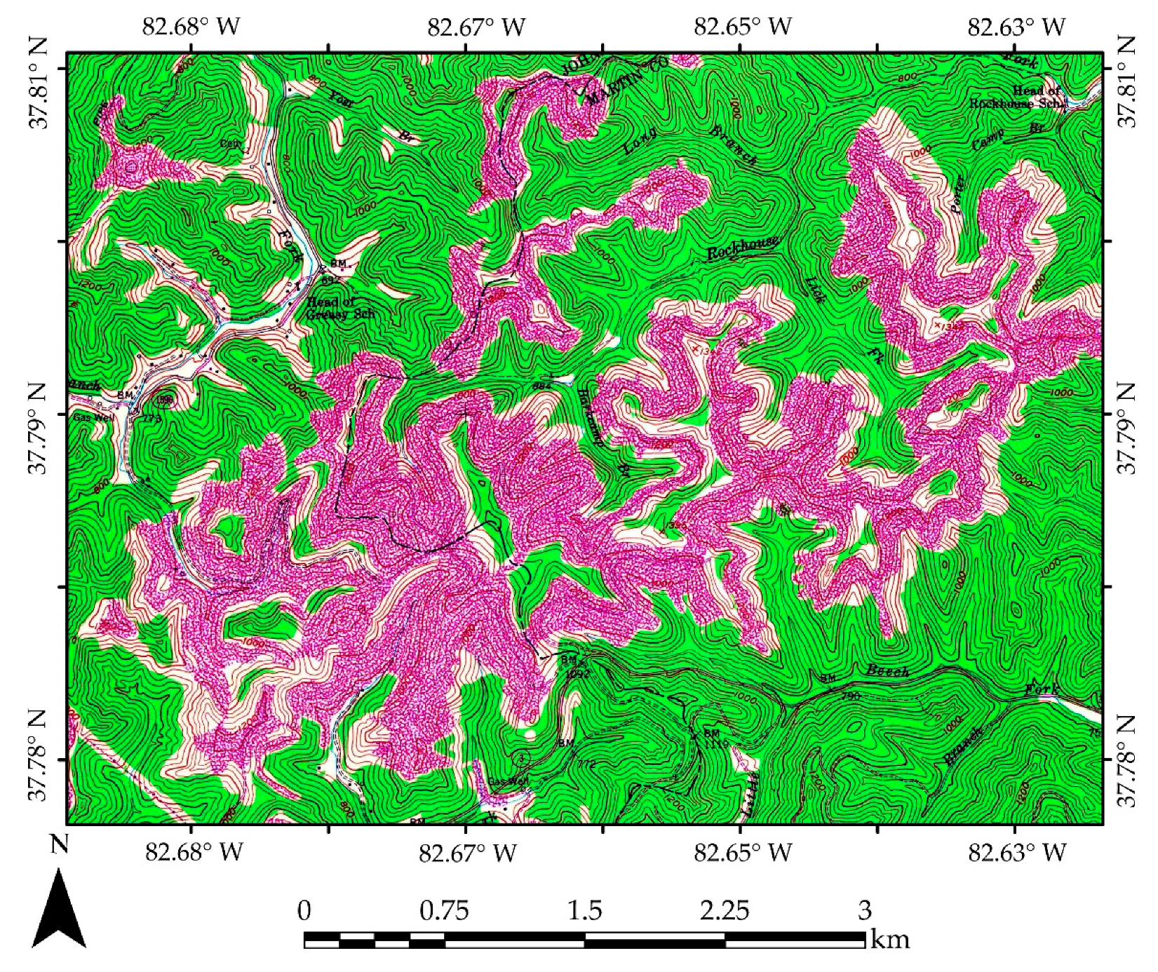
1.1. Topographic Maps

The first USGS topographic map was produced in 1879; however, the number of maps produced was limited until the 1940s and 1950s when aerial photo acquisition and photogrammetric methods became routine for deriving elevation data from overlapping stereo images. The largest-scale maps produced for the entire conterminous US, which are used in this study, were produced on a 1:24,000 scale and span 7.5 min of latitude and longitude, known as 7.5-minute quadrangles [27]. When the program ended in 2006, it was replaced by the US Topo program, which generates digital maps and associated geospatial databases. Paper maps from the prior program were scanned and georeferenced into the National Map’s Historical Topographic Map Collection (HTMC) and can be accessed as digital raster graphics (DRGs) for use in geographic information systems [28,29,30,31]. Currently, maps can be viewed and downloaded using topoView, which includes an interactive web map (https://ngmdb.usgs.gov/topoview/) [32].

Historic topographic maps document a wide variety of mining and prospecting features including pits, strip mines, disturbed surfaces, mine dumps, quarries, and tailings using point symbols, areal symbols, and text, which are the product of manual photograph interpretation and some field validations. Areas of surface mining disturbance are generally symbolized using a generic brown and/or pink pattern (see Figure 1) with some more unique symbols for specific features, such as tailings [23]. Such areal, thematic features are the focus of this study.

1.2. Surface Mine Mapping

Despite the large database of historic cartographic representations of mining, much effort has been placed on the use of remotely sensed data for mapping and monitoring surface mining and subsequent reclamation. For example, Townsend et al. [33] documented surface mine extent change in portions of central Appalachia from 1976 to 2006 using a Landsat time series, while Pericak et al. [34] and Xiao et al. [35] used Landsat data and Google Earth Engine cloud-based computation to map surface mining in the mountaintop mining region of the eastern US and the Shengli coalfields of Inner Mongolia, respectively. Also using Landsat data, Sen et al. [36] applied disturbance/recovery trajectories for differentiating mining and mine reclamation from other forest displacing practices. Several studies have compared commercial satellite imagery, aerial orthophotography, and the combination of imagery and light detection and ranging (LiDAR) for mapping of mining and mine reclamation [37,38,39,40].

Despite the existing research on mine mapping from remotely sensed data, a review of the literature suggests that there is a lack of studies focused on extracting surface mine features from topographic maps and other cartographic representations. In fact, research on the use of machine learning (ML) or DL to extract features from topographic maps is generally limited. Li et al. [24] explored the recognition of text on topographic maps using DL while Uhl et al. [25] investigated the mapping of human settlements from maps using CNNs. Lui et al. [41] explored CNNs for the general segmentation of topographic maps. There has been some success in applying DL methods to other types of digital data, beyond the primary focus on multispectral satellite or aerial imagery. For example, DL has been applied to the detection of features from digital terrain data; Behrens et al. [42] investigated the application of digital elevation data and DL for digital soil mapping while Trier et al. [43] investigated the mapping of archeological features from LiDAR data. In a mining-related study, Maxwell et al. [44] used LiDAR-derived slopeshades and the Mask Regional-CNN (Mask R-CNN) DL algorithm for detecting instances of valley fill faces, which are an artificial landform resulting from mountaintop removal mining and reclamation practices. As these studies highlight, DL methods have been shown to be of value for mapping and extracting features from a variety of geospatial data layers, suggesting that further investigation of their application to historic topographic maps is merited.

1.3. Deep Learning Semantic Segmentation

Extraction of thematic information from geospatial data is both a common operational task and an active area of research [45]. Supervised classification, which relies on user-provided training data, using ML algorithms is often undertaken since these methods have been shown to be more robust to complex feature space than parametric methods [46,47]. However, the incorporation of spatial context information is limited when the pixel is used as the unit of analyses and no textural measures are included as predictor variables [48,49]. To overcome this lack of spatial context, especially when high spatial resolution data are used, geographic object-based image analysis (GEOBIA) first groups adjacent pixels into objects or polygons based on similarity. These regions then become the unit for subsequent analysis and classification [48,50,51]. CNN-based DL for semantic segmentation further expands the incorporation of spatial context information, and offers a natural extension of prior methods [52,53,54,55].

DL is an extension of artificial neural networks (ANNs). An ANN consists of neurons organized into layers where input layers represent input predictor variables, such as image bands, while output layers represent the desired output, such as land cover categories. Between the input and output layers are one or more hidden layers containing multiple neurons. Within the network, connections between neurons have associated weights that can be learned or updated. By applying a bias and a non-linear activation function while iteratively adjusting the weights through multiple passes, or epochs, on the training data while monitoring a loss metric, patterns in the data can be learned to make new predictions [46,56,57]. DL expands upon this ML framework to include many hidden layers and associated nodes (i.e., tens or hundreds), which can allow for the modeling of more complex patterns and a greater abstraction of the input data [52,53,54,55].

DL and its applications in remote sensing science and image analysis have expanded greatly with the inclusion of convolutional layers, which allow CNNs to learn spatial patterns by updating weights associated with spatial filters or kernels. These learned filters then pass over the image as a moving window to perform convolution and generate spatial abstractions of the data, or feature maps. When applied to DL, it is common for hundreds of such filters to be learned. Initially, CNNs were applied to scene labelling problems where an entire image is categorized. Advancements in CNNs have allowed for semantic segmentation, where each pixel is classified, similar to traditional remote sensing classification methods, or instance segmentation, where individual instances of a class are differentiated [52,53,54,55]. We make use of semantic segmentation in this study.

Fully convolutional neural networks (FCNs) offer one means to perform semantic segmentation with CNN-based architectures using a combination of convolution and deconvolution with up-sampling (i.e., increasing the size of the data array that represents the image). Example FCNs include SegNet [58], which was originally developed for semantic segmentation of digital photographs and introduced in 2017, and UNet [59,60,61], which was developed for segmentation of medical imagery and introduced in 2015. In this study, we use a modified version of UNet.

A conceptualization of a generic UNet is provided in Figure 2. First, in the convolution, contracting, or encoder component, spatial patterns are modeled at multiple scales by iteratively adjusting weights associated with a series of 3 × 3 2-dimensional (2D) convolutional layers and by applying 2 × 2 max pooling, which decreases the size of the data array by returning the maximum value of the feature maps within 2 × 2 pixel windows. This allows for spatial patterns to be learned at multiple scales since feature maps generated by the prior convolutional layer are used as input to the subsequent layer following the max pooling operation. Next, these same feature maps are used to convert the data back to the original dimensions using 2D deconvolution to output a semantic, or pixel-level, classification from the reconstruction. This is the deconvolution, expanding, or decoding component [59,60,61].

In Figure 2, the example UNet accepts training data as image chips with dimensions of 128 pixels (height) × 128 pixels (width) × 3 channels (for example, red, green, and blue). As the data are fed through the encoder component, 3 × 3 2D convolution is used to learn spatial filters, and the dimensions of the data array decrease (128 → 64 → 32 → 16 → 8) as a result of the max pooling operations while the number of filters increases (64 → 128 → 256 → 512 → 1024). In the decoding component, the size of the array increases as a result of 2 × 2 2D deconvolution applied to the feature maps learned in the encoding component while the number of filters decreases. In the final phase of the architecture, 64 channels or feature maps are used as input to perform a classification at each pixel location, where each pixel location is treated as a vector containing 64 values or predictor variables. The output is a probability of each pixel belonging to each of the defined classes, with the total of all class probabilities at each pixel location summing to 1.

UNet and other semantic segmentation methods have been applied to a variety of feature extraction and classification problems and have also been applied to a variety of geospatial and remotely sensed data. For example, modifications of UNet have been applied to the mapping of general land cover change [62], coastal wetlands [63], palm trees [64], cloud and cloud shadows [65], urban buildings and change detection [66,67,68], roads [69], and landslides [70]. Generally, UNet and other FCNs have shown great promise due to their ability to model complex spatial patterns and context while generating data abstractions that generalize well to new data [54,55]. Given the complex patterns present in topographic maps, where features may be overprinted with contour lines, points symbols, and/or text, and inconsistencies between different scanned topographic maps in regard to tone, hue, contrast, and/or sharpness, we hypothesize that this is an optimal method to explore for this mapping problem.

2. Materials and Methods

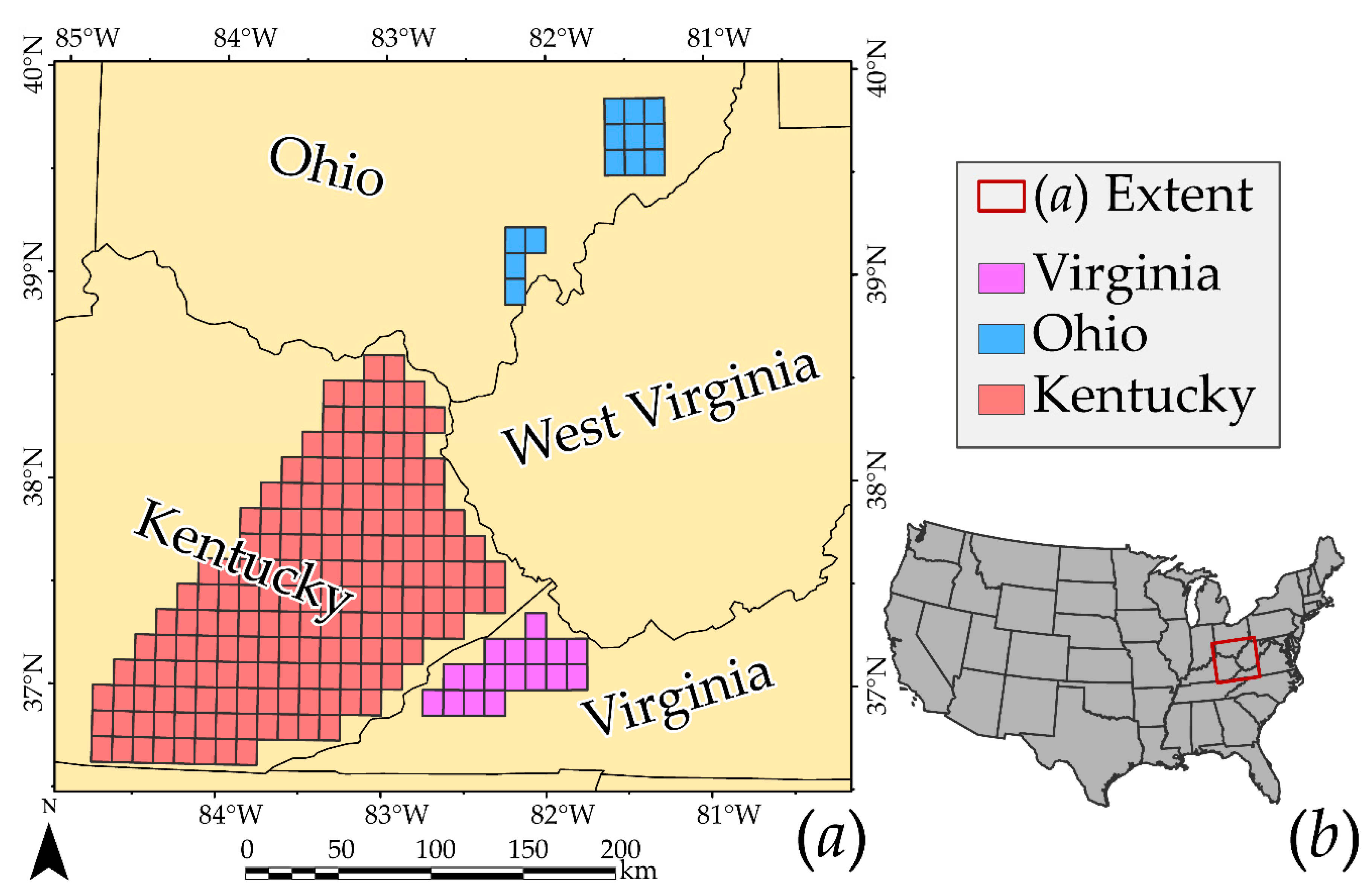
2.1. Study Areas and Input Data

In this study, we focus on the surface coal mining region of Appalachia in the eastern US due to the availability of historic topographic maps and training data and an abundance of historic surface mine disturbance. As shown in Figure 3, eastern KY is the primary area of study. Within this region, 100 7.5-minute quadrangles were selected (

Table 1. Number of unique 1:24,000-scale, 7.5-minute topographic quadrangles within each dataset. A unique map is defined based on a SCANID. The Unique Quads column provides the number of unique quadrangle names in each dataset. The chips columns represent the number of 128-by-128 pixel chips in each dataset that contain mining and/or not mining pixels, only no mining pixels, and the total number of chips. The compilation years of the oldest and newest maps within each dataset are also provided.

Dataset	Unique Maps (SCANID)	Unique Quads (Name)	Mining and Absence Chips	Absence Only Chips	Total Chips	Oldest Year	Newest Year
KY Training	84	70	17,792	12,600	30,392	1949	1980
KY Testing	18	15	2588	2700	5288	1953	1992
KY Validation	20	15	3849	3000	6849	1951	1992
OH Validation	23	10	6849	3450	10,299	1960	2002
VA Validation	25	12	12,140	3750	15,890	1957	1968

KY = Kentucky, OH = Ohio, and VA = Virginia.

). Since multiple maps can be generated for each quadrangle representing different dates and historic conditions, a total of 122 maps were included in the study. Any topographic map that did not include any mapped surface mine disturbance was removed. In order to assess how well the trained models generalize to different topographic maps and new geographic extents, we selected 23 additional topographic maps in OH and 25 in VA based on the prevalence of surface mine features. A total of 170 historic topographic maps were included in the study.

Example mine extents were obtained from the publicly available USGS GGGSC prospect- and mine-related features database. This is an ongoing project, and data are not currently available for all historic maps and states. For example, data for WV is not yet complete [23]. This database contains manually digitized point and polygon features interpreted from mine symbols on historic topographic maps available in the HTMC. Examples of the historic topographic maps and mining features data are shown in Figure 4. We only used polygon features digitized from 1:24,000-scale maps in this study. Also, any features categorized as a pond were removed from the dataset, and we maintained all features that were denoted using the standard brown or pink “surface disturbance” pattern or symbols associated with tailings. In the public HTMC database, each historic topographic map is identified with a unique SCANID. We found that it was not possible to simply match the digitized features with the correct map based on this identifier, as features near quadrangle boundaries were not re-digitized if they were already captured in adjacent quads or if the features were captured in a prior version of the topographic map and did not change. So, all features that intersected the extent of the quadrangle were extracted and then manually inspected for all 170 maps. Features that were not present on the map were removed, and any missing features were added; however, missing features were a rare occurrence, as the database was very comprehensive.

DL models that make use of CNNs require that training data be provided as small image chips. When semantic segmentation is being performed, labels must be provided as raster masks where each category is assigned a unique code or cell value [52,53,54,55]. Image chips and associated label masks were generated using the Export Training Data for Deep Learning Tool in the ArcGIS Pro software environment [71,72]. Chips were produced at a size of 128-by-128 pixels, as this allowed for the generation of a large number of chips, the use of a large batch size during training and validation, and did not overwhelm the computational resources. Given the large number of available chips, and to decrease correlation amongst the data, no overlap was used so that each chip covered a unique extent. Moreover, only full chips were produced. Thus, chips from near the edge of maps, which do not allow for a complete set of 128-by-128 rows and columns of data, were not included. All chips that contained at least some cells occurring in the historic mine extents were used. In order to incorporate a variety of examples of the background, absence, or “not mining” class, we randomly selected an additional 150 absence-only chips from each topographic map. This subsample from the complete dataset of absence-only chips was selected to reduce class imbalance in the training process. Table 1 above summarizes the number of chips used in each dataset. In total, the model was trained using 30,392 examples (KY Training) and evaluated at the end of each training epoch with 5288 chips (KY Testing). To validate the final model, 6849 chips were withheld from the KY data (KY Validation); these chips did not overlap with the training or testing data. We also validated in the new regions within OH and VA using 10,299 and 15,890 chips, respectively (OH Validation and VA Validation). Example image chips and associated masks are shown in Figure 5.

In order to minimize autocorrelation in the training, testing, and validation datasets, all image chips from the same SCANID were included in the same partition. Moreover, all chips from the same quadrangle, as identified by the quad name, were included in the same partition. These divisions were determined using random sampling.

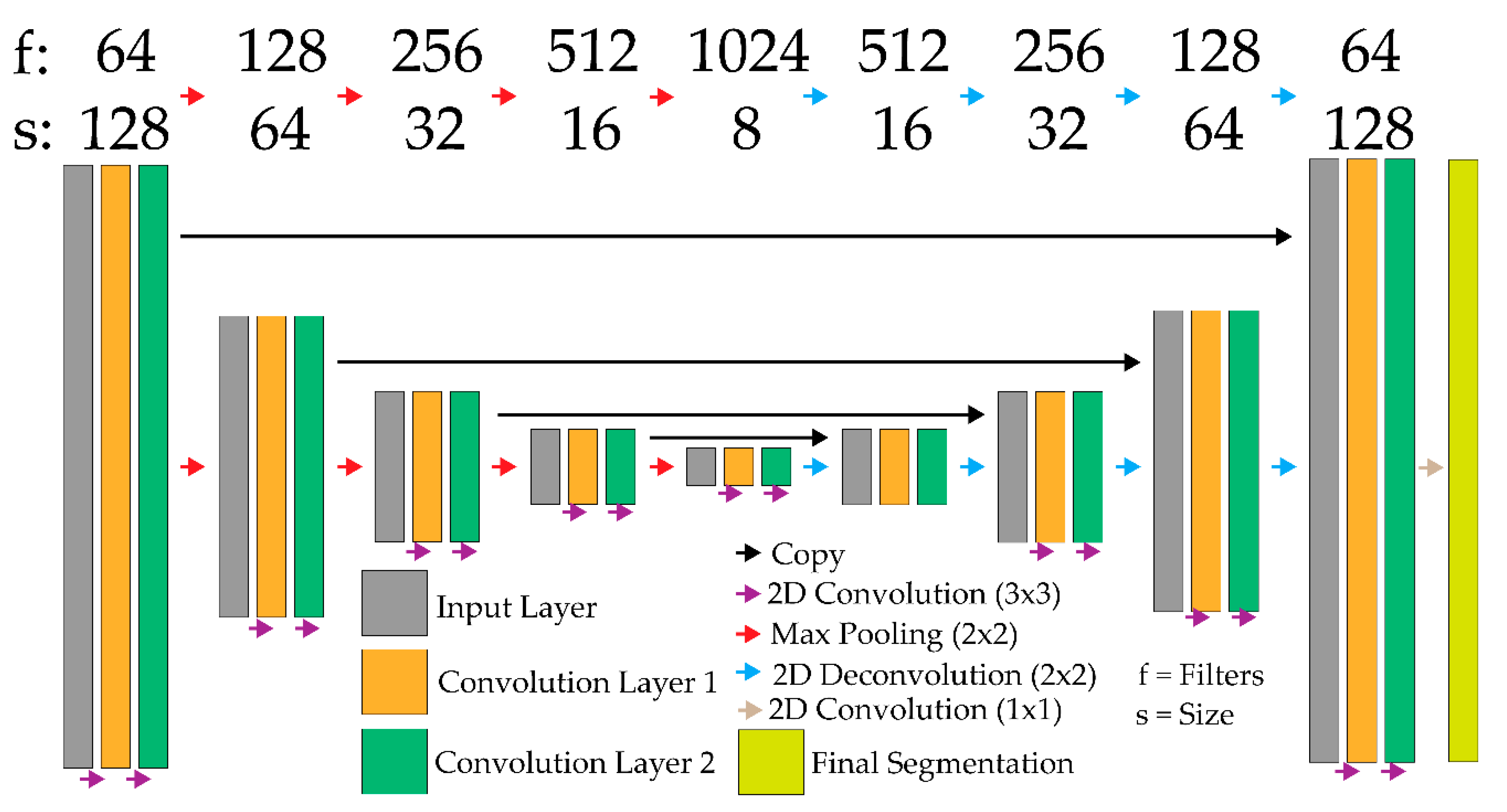
2.2. Modeling Training

DL model training and assessment were conducted using the R statistical and data science computational environment and language [73]. Specifically, models were generated using the keras [74] and tensorflow [75] packages. The keras package interfaces with the Keras Application Programming Interface (API) [76], which is written in Python [77] and can interface with several DL and tensor math backends, including Google’s TensorFlow [78]. The reticulate package [79] allows for an interface between R and Python, and was used to allow the keras package to make use of the Python API. For image manipulation and preparation, we used the magick package [80], which provides bindings to the ImageMagick open-source image processing library. In order to implement and modify UNet specifically, we referenced the UNet example provided by RStudio and available on GitHub and as part of the online keras package documentation [81,82]. All experiments were conducted on a Microsoft Azure virtual machine, which provided access to an NVIDIA Tesla T4 graphics processing unit (GPU).

The UNet model used in this study is described in

Table 2. Semantic segmentation algorithm architecture used in this study and modified from UNet.

Parameter	Value
Trainable Number of Parameters	34,527,041
Non-Trainable Number of Parameters	13,696
Input Image Size (Height × Width × Channels)	128 × 128 × 3
Kernel Size	3 × 3
Padding	“Same”
Max Pooling	2 × 2
Max Pooling Stride	2 × 2
Number of Downsampling Blocks	4
Number of Upsampling Blocks	4
Convolutional Layers per Block (Downsampling)	2
Convolutional Layers per Block (Upsampling)	3
Number of Filters	64, 128, 256, 512, 1024
CNN Activation	Leaky ReLU
Classification Activation	Sigmoid
Loss Metric	Dice Coefficient Loss
Optimizer	AdaMax

. Similar to the default architecture, we used 4 downsampling blocks in the encoder and 4 upsampling blocks in the decoder. The downsampling blocks each contained 2 convolutional layers, while the upsampling blocks contained 3. The default number of filters per block and kernel size were maintained. The architecture was designed to accept input tensors of shape 128 × 128 × 3 (height, width, channels) and differentiate two classes: mining features, coded to 1, and not-mining features, coded to 0. Since this is a binary classification problem, a sigmoid activation function [83] was used in the final layer, which resulted in a probabilistic prediction between 0 and 1, where 1 represents a predicted high likelihood of a mine feature occurring at the pixel location. In order to maintain the size of the arrays, padding was used along with a max pooling size and stride of 2 × 2. A total of 34,527,041 trainable parameters were included in the model.

Some changes were made to the default UNet architecture. First, we used the leaky rectified linear unit (ReLU) activation function as opposed to a traditional ReLU in the convolutional layers to avoid “dying ReLU” issues [84]. We also used the AdaMax optimizer [85] instead of Adam (Adaptive momentum estimation) or RMSProp (Root Mean Square Propagation) and included a callback to reduce the learning rate if the loss plateaued for more than 5 epochs. Lastly, we used Dice coefficient loss as opposed to binary cross-entropy loss due to issues of class imbalance and our desire to balance omission and commission error rates for the mine features class [86,87,88].

The model was trained for 100 epochs using all the training examples in batches of 32 image chips, and the final model was selected as the model with the lowest Dice coefficient loss for the KY Testing data. The training examples were randomly shuffled between each epoch, and random data augmentations were included to increase the data variability and combat overfitting. Specifically, image chips were randomly flipped left-to-right and/or up-and-down. Slight random adjustments of brightness, contrast, saturation, and/or hue were also applied. Lastly, batch normalization was implemented for all convolutional layers. The model took roughly 24 h to train on the Microsoft Azure virtual machine using the available GPU.

2.3. Prediction and Model Validation

Once a final prediction was obtained, the keras package was used to predict the withheld validation image chips in KY, OH, and VA and to calculate assessment metrics. We also developed a custom R script to apply the prediction to entire topographic maps, which broke the input data into 128-by-128 pixel arrays, used the model to predict each subset, then merged the results to reproduce the topographic map extent. In order to remove poor predictions near edges of each chip, the outer 20 rows and columns of each chip were removed, and a 50% overlap between adjacent chips was applied so that only the center of each chip was used in the final, merged prediction. Any cell with a mine feature probability higher than 0.5 was coded to the mine features class while all other cells were coded to the not mine feature class. Using our custom script, an entire topographic map could be predicted in roughly 15 minutes.

For validation, we relied on common binary classification accuracy assessment metrics including precision, recall, specificity, the F1 score, and overall accuracy.

Table 3. Example binary confusion matrix and associated terminology.

		Reference Data
		True	False
Classification Result	True	TP	FP
	False	FN	TN

describes the terminology used to define these metrics. True positive (TP) samples are those that are in the positive class and are correctly mapped as positive, in this case mine features, while false positives (FPs) are not in the positive class but are incorrectly mapped as a positive. True negatives (TNs) are correctly mapped as negative, while false negatives (FNs) are mapped as negative when they are actually positive. Precision (Equation (1)) represents the proportion of the samples that is correctly classified within the samples predicted to be positive, and is equivalent to the user’s accuracy (1—commission error) for the positive class. Recall or sensitivity (Equation (2)) represents the proportion of the reference data for the positive class that is correctly classified, and is equivalent to producer’s accuracy (1—omission error) for that class. The Dice coefficient or F1 score (Equation (3)) are equivalent and represent the harmonic mean of precision and recall, while specificity (Equation (4)) represents the proportion of negative reference samples that is correctly predicted, and is thus equivalent to the producer’s accuracy for the negative class. Lastly, overall accuracy or binary accuracy (Equation (5)) represents the proportion of correctly classified features [86,87,88,89].

$$\mathrm{Precision} = \frac{\mathrm{TP}}{\mathrm{TP} + \mathrm{FP}}$$

(1)

$$\mathrm{Recall} \mathrm{or} \mathrm{Sensitivity} = \frac{\mathrm{TP}}{\mathrm{TP} + \mathrm{FN}}$$

(2)

$$\mathrm{Dice} \mathrm{Coefficient} \mathrm{or} \mathrm{F}1 \mathrm{Score} = \frac{2 \times \mathrm{Precision} \times \mathrm{Recall}}{\mathrm{Precision} + \mathrm{Recall}}$$

(3)

$$\mathrm{Specificity} = \frac{\mathrm{TN}}{\mathrm{TN} + \mathrm{FP}}$$

(4)

$$\mathrm{Overall} \mathrm{Accuracy} \mathrm{or} \mathrm{Binary} \mathrm{Accuracy} = \frac{\mathrm{TP} + \mathrm{TN}}{\mathrm{TP} + \mathrm{TN} + \mathrm{FP} + \mathrm{FN}}$$

(5)

Model assessments were performed using the validation image chips in KY, OH, and VA, a total of 33,038 examples. Given that these chips did not incorporate all areas of the topographic maps, we also calculated assessment metrics for each validation topographic map. We argue that this is a more robust validation of the map products, as the entire extent of each map is assessed as opposed to just chips containing surface mine features or a subset of randomly selected absence-only chips. The model was validated on a total of 68 topographic maps that were not include in the KY Training or KY Testing sets.

2.4. Sample Size Comparisons

In order to assess the impact of sample size on model performance and model generalization, we also trained models on subsets of the available KY Training dataset. This was accomplished by randomly selecting all chips assigned to a defined number of topographic maps. In the random selection, the probability of selection was weighted by the relative land area of mining in each topographic map, since it was assumed that analysts undertaking manual digitizing over a small set of available maps would select maps with many mining examples present. In order to assess model variability at different sample sizes, 5 random subsets of the training topographic maps and associated chips were selected for 2, 5, 10, and 15 topographic maps each, or a total of 20 models. All models were trained for 100 epochs using the same settings used for the model that incorporated all KY Training image chips. We also included the same random image augmentations. The model, which consists of the learned weights at the end of the training epoch, with the largest Dice coefficient for the KY Testing data was selected as the final model for each sample. We also evaluated the results by predicting to the KY, OH, and VA validation datasets. We did not perform a validation at the topographic map scale due to computational constraints and processing time required to predict all the validation topographic maps using all 20 models.

3. Results

Figure 6 summarizes the results of the training process for the KY Training and KY Testing datasets for the 100 training epochs. As the model iterated through the KY Training set and the weights were updated, the training accuracy continued to increase while the pattern for the testing data was more variable or noisy. However, the overall trend was that accuracy for both the training and testing datasets stabilized quickly (i.e., after roughly 30 epochs). Following the initial rapid improvement, small gains in the training data accuracy were observed while the testing data performance stopped improving. Generally, overfitting was not observed. Performance on the KY Testing data stabilized with a Dice coefficient of 0.960 to 0.970 (Figure 6a), and the best performance on the testing data occurred at epoch 75, which was selected as the final model for predicting to the three validation datasets. Also, precision and recall were similar, suggesting a balance between errors of commission and omission for the mining features class (Figure 6c,d).

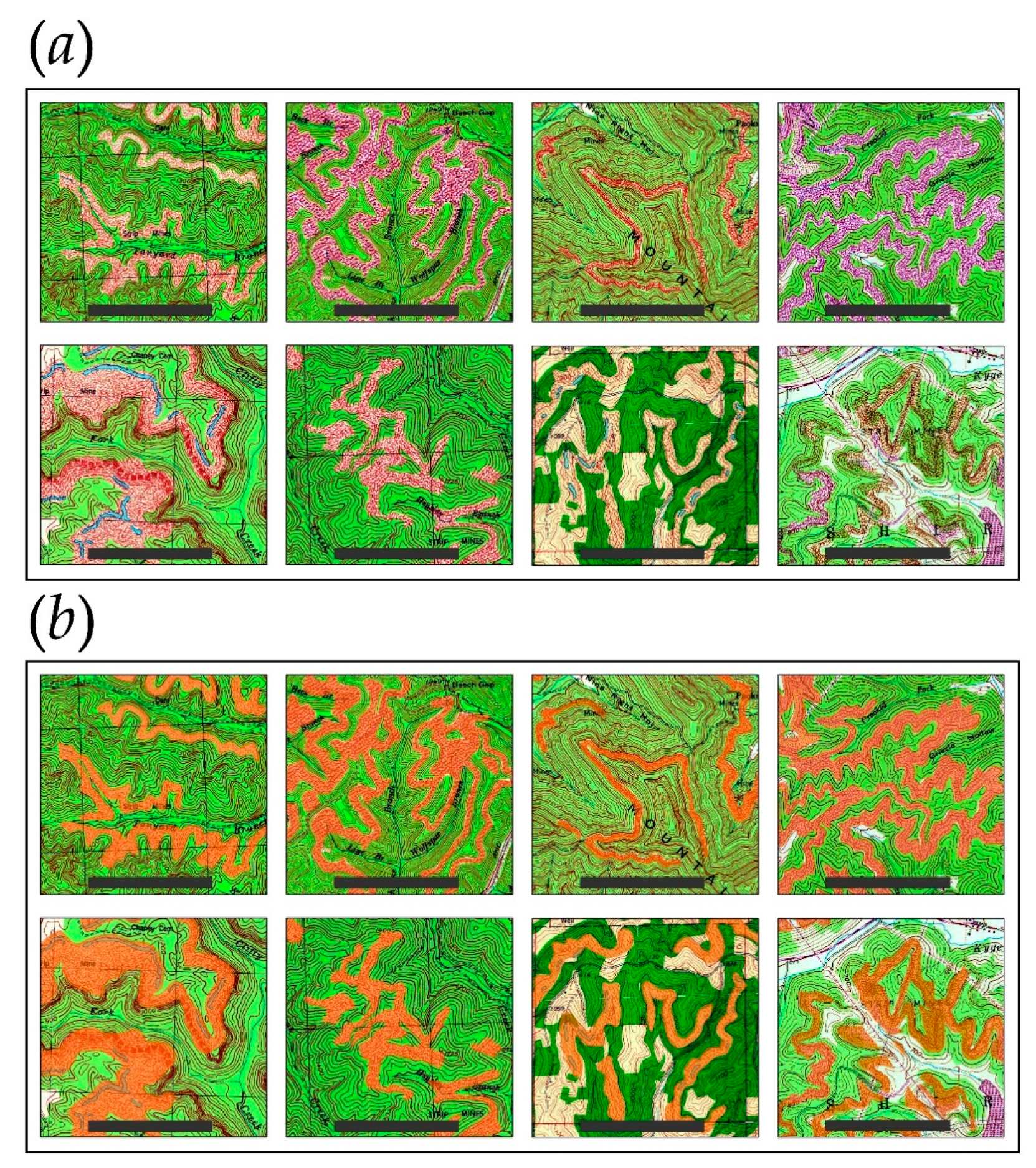
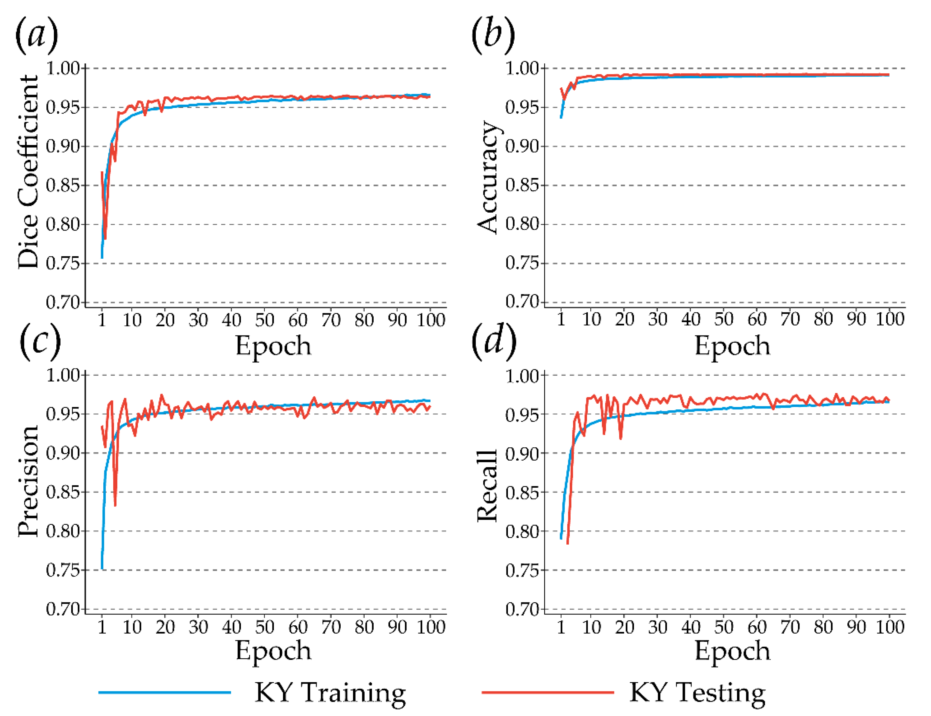
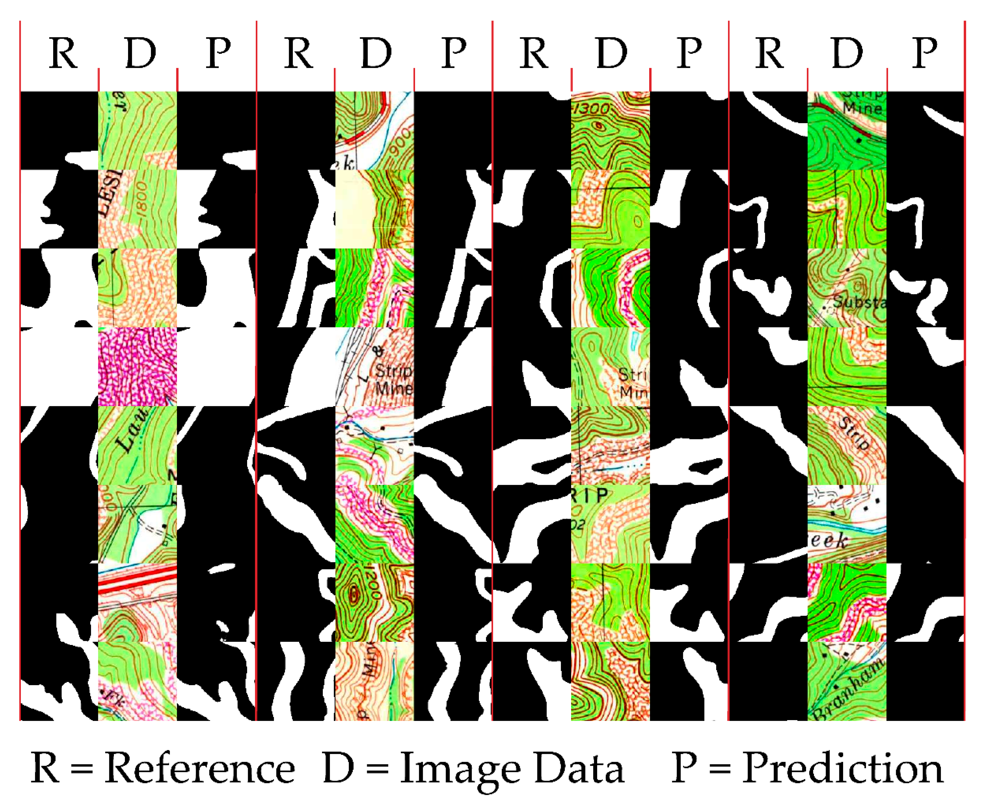
3.1. Chip-Based Assessment

Figure 7 provides example results for a random selection of image chips from the KY Validation dataset. This visualization generally suggests the model can identify most of the mine areas, based on the strong similarities between the reference and predicted masks, despite the presence of clutter such as text, other annotated features, and/or contour lines. Some errors of commission, or false positives, were observed, such as the inclusion of features that used similar thematic symbology. For example, some highways and small ponds were incorrectly detected.

Table 4. Validation results using image chips. N = number of chips in the dataset.

Dataset	Dice/F1 Score	Precision	Recall	Accuracy	N
KY Training	0.959	0.967	0.951	0.990	30,392
KY Testing	0.965	0.967	0.963	0.993	5288
KY Validation	0.949	0.954	0.944	0.989	6849
OH Validation	0.894	0.966	0.835	0.963	10,299
VA Validation	0.837	0.971	0.741	0.942	15,890

summarized the assessment results for all datasets as calculated using the image chips. Assessment results for the KY Training data were included for comparison; however, this assessment could be misleading due to overfitting. Generally, overall or binary accuracies were high, which we attribute to the large number of background pixels in the image chips. For the KY Testing and Validation data, precision and recall were generally well balanced, whereas precision rates were higher for the OH and VA validation data in comparison to recall, which suggest higher levels of omission error than commission error when the model is generalized to new geographic areas. This could potentially be attributed to differences in the representation or presentation of mine features in the new data. For the KY Testing and KY Validation data, the Dice coefficients or F1 scores were above 0.944. For the OH and VA validation chips, the Dice coefficients were 0.894 and 0.837, respectively. Similar to the results of Maxwell et al. [44], who investigated the mapping of valley fill faces from high spatial resolution digital elevation data, these results suggest some reduced performance when DL models are used to predict to new geographic extents; however, performance is still strong, suggesting that the model is valuable for predicting new data.

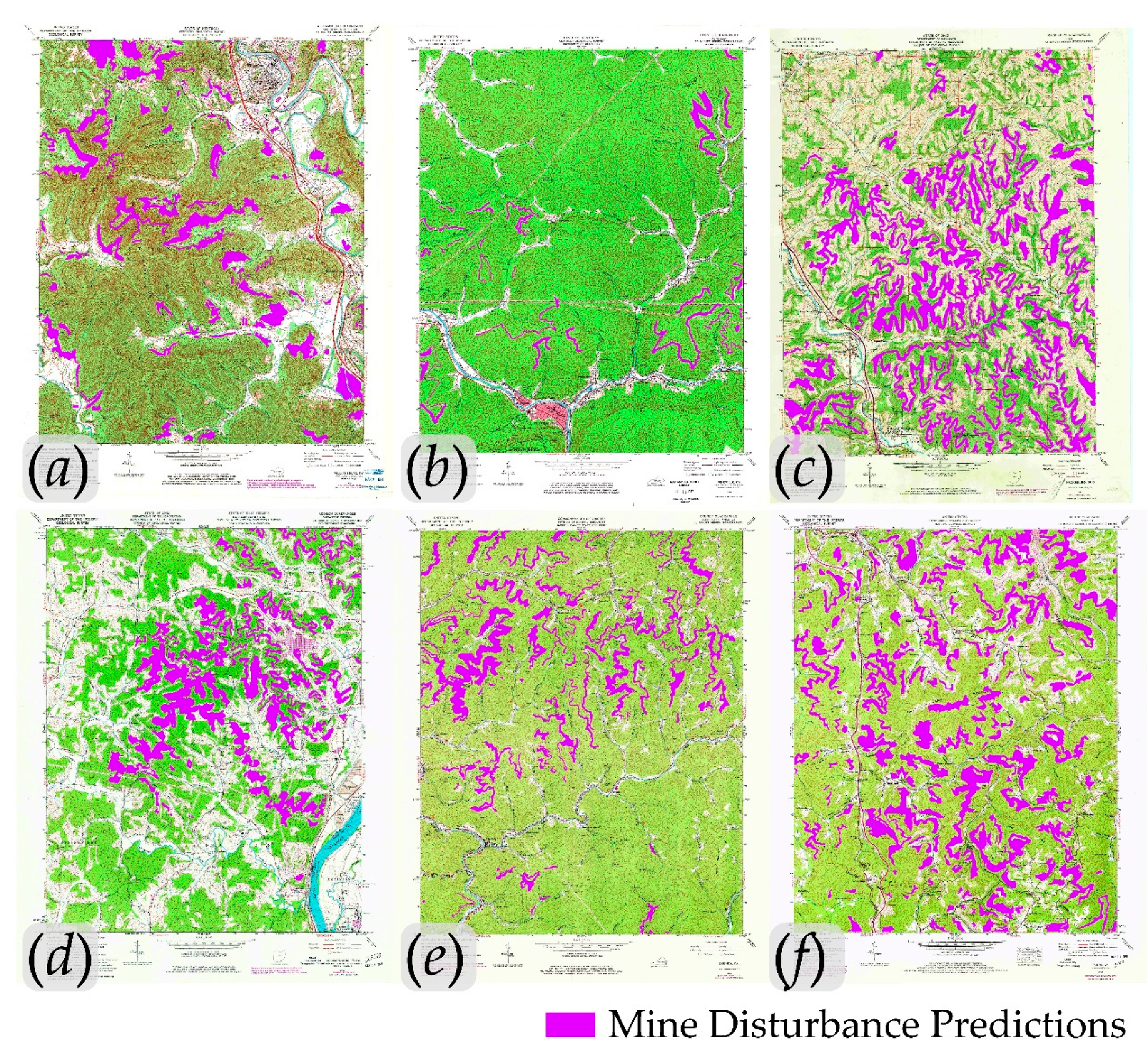
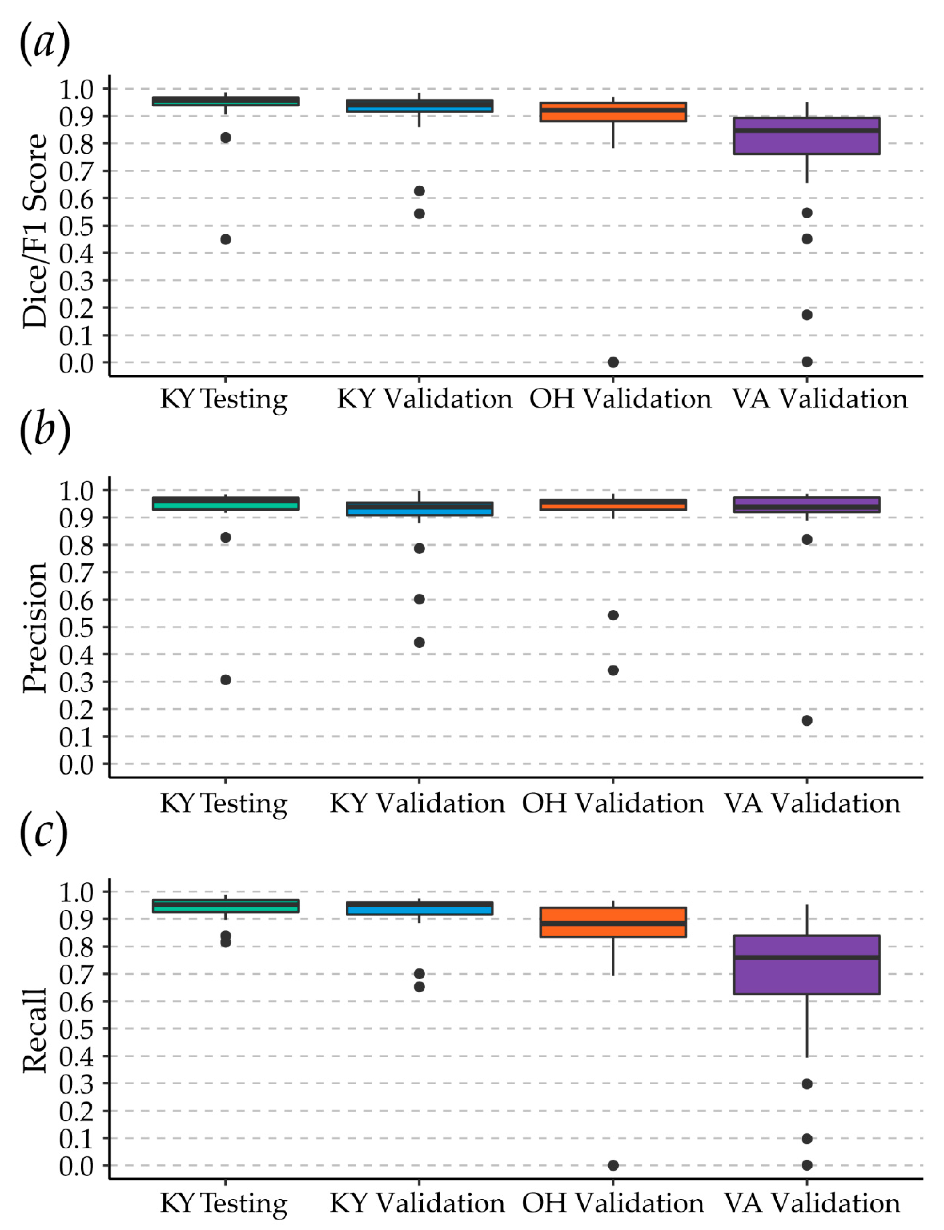
3.2. Topographic Map-Based Assessment

Table 5. Validation results using topographic maps. Values represent the mean values for all topographic maps in the set. N = number of image chips in the dataset.

Dataset	Dice/F1 Score	Precision	Recall	Specificity	Accuracy	N
KY Testing	0.920	0.914	0.939	0.999	0.999	18
KY Validation	0.902	0.891	0.917	0.999	0.998	20
OH Validation	0.837	0.905	0.811	0.998	0.992	23
VA Validation	0.763	0.910	0.686	0.998	0.983	25

summarizes the assessment results for the topographic map-based assessment while Figure 8 provides some example results as two topographic maps from each state validation dataset. These results generally agree with those obtained using the chip-based validation. Strongest performance was generally observed when predicting to new topographic maps within KY (i.e., the KY Testing and KY Validation datasets). Overall accuracy and specificity were generally high, suggesting that most of the background pixels were correctly classified. For the OH and VA validation datasets, recall was generally lower than precision, suggesting higher levels of omission error. For all datasets, precision was above 0.890, suggesting low commission error rates.

Figure 9 further summarizes the distribution of model performance for the testing and validation data. Generally, there was more variability in the prediction of the VA data than the other datasets. However, all datasets had some outlying topographic maps where model performance was poor. Visual inspection of these poorly classified maps suggest that they were obtained for maps with a small percentage or land area of surface mining where small proportions of omission or commission error had large weight and thus greatly impacted the reported metrics.

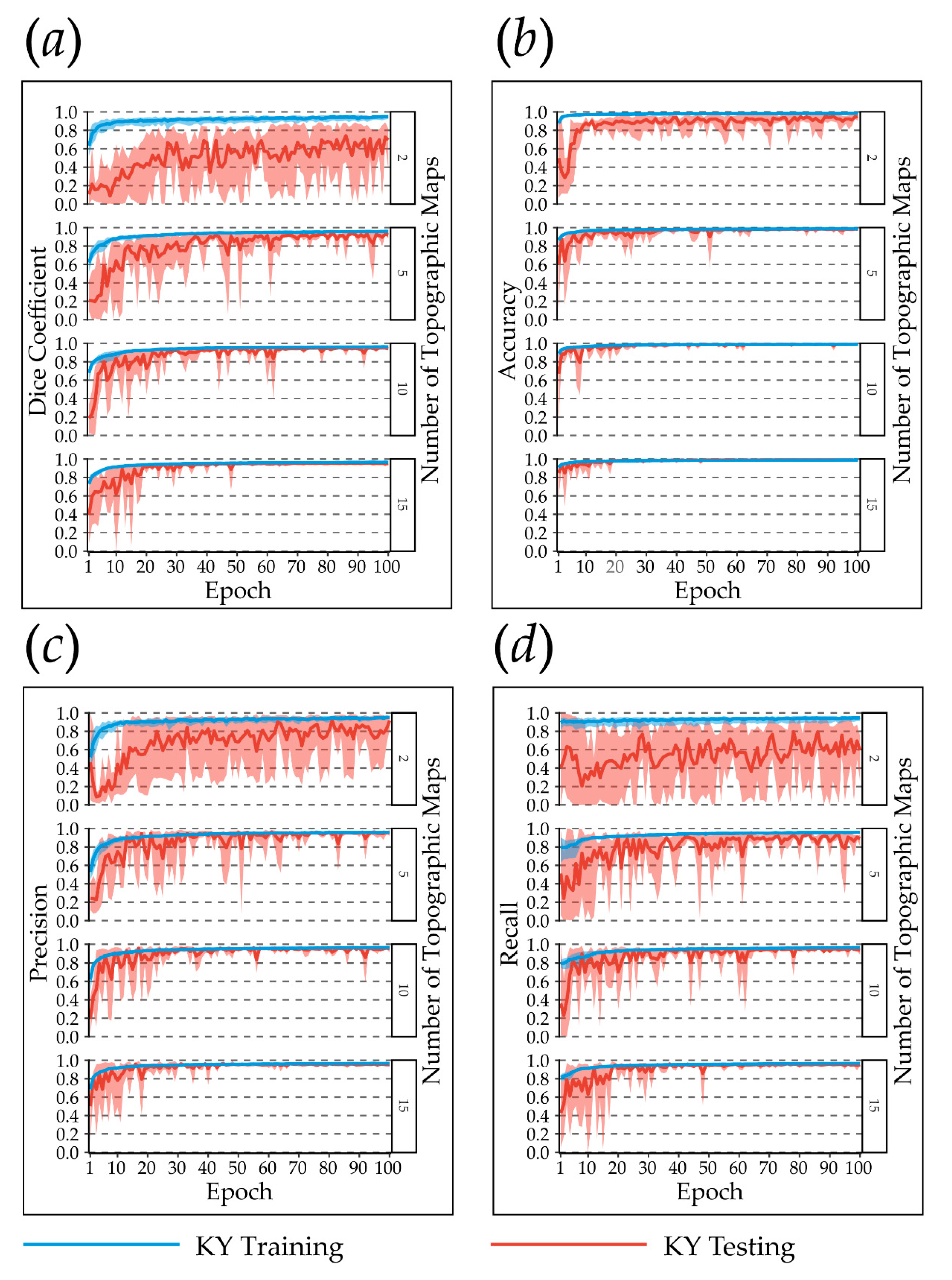
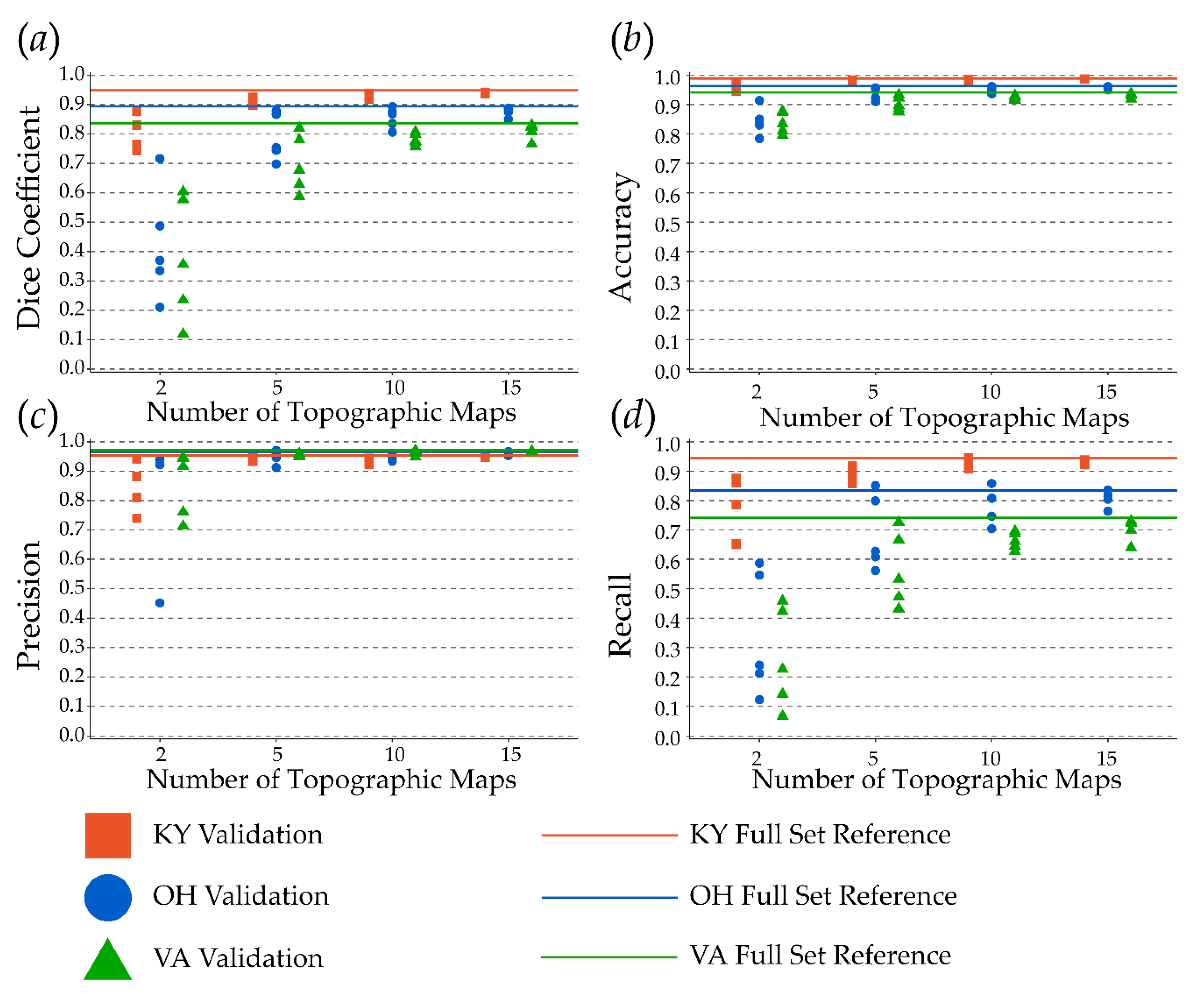
3.3. Sample Size Comparisons

Figure 10 and Figure 11 below describe the results of the sample size comparison. Figure 10 shows the changes in performance metrics for predicting the KY Training and KY Testing chips by epoch. Generally, reducing the number of topographic maps used to train the model decreased model performance and increased variability between the different random subsets, as represented with the ribbons in the graphs that represent the range at each epoch. When chips from only two topographic maps were used, the Dice coefficient, precision, and recall (Figure 10a–c) varied greatly at the same training epoch, even after many training iterations. Also, the model generalized poorly to the KY Testing data; for example, the mean Dice coefficient for all five models across all epochs never rose above 0.800 for the KY Testing set but stabilized above 0.950 for the KY Training data. When the number of topographic maps was increased to 10 or 15, variability between the models decreased, overfitting was reduced, based on a comparison between the training and testing results, and the performance approached that obtained when using the entire training datasets of 84 maps and associated chips. This generally suggests that quality results can be obtained with a smaller dataset, which reduces manual labor requirements for training and validating DL models and adds practicality to including DL semantic segmentation into production-level data generation over large spatial extents and/or large volumes of data.

Adding to the results summarized in Figure 10, Figure 11 shows the results when the models trained with a reduced sample size were used to predict to the KY, OH, and VA validation sets. Similar to the results for the model trained with all the training samples, these models generalized better to the KY Validation data as opposed to the OH and VA sets. For all sample sizes, the performance for the VA data was the lowest. Variability between different random sets tended to decrease as the number of topographic maps used in the training process increased. Models using 15 topographic maps approached the performance levels reached with the full training dataset in which chips were derived from 84 topographic maps. For example, the average Dice coefficients for the 15 topographic map models were 0.940, 0.875, and 0.813 for the KY, OH, and VA validation sets, respectively. For comparison, the model using all the training samples yielded Dice coefficients of 0.949, 0.894, 0.837 for the same validation sets. This generally suggests that, although more samples can improve the results, a reduced sample size can be adequate, which would minimize manual labor requirements for generating and validating models.

4. Discussion

Based on an evaluation on multiple datasets, our results suggest that DL semantic segmentation can be successfully applied to historic topographic maps to extract the extent of mining-related landscape disturbance. Although model performance decreased when generalized to new geographic extents, performance was still strong with Dice coefficients above 0.760. Practically, DL semantic segmentation can offer a means to reduce workloads and manual digitizing time for deriving vector geospatial data from historic, georeferenced topographic maps. This is especially true given that a reduced sample size can still yield accurate results, as demonstrated by our sample size reduction experimentation. Further, errors when generalizing to new data and geographic extents were dominated by omission error, as measured with recall, and precision remained above 0.890 for all datasets, even when the number of training topographic maps in the datasets were reduced to 15. In general, we would recommend large-area mapping projects to take advantage of DL methods to decrease manual labor and shorten project timelines. Results from DL models can then be further refined using manual interpretation by digitizing missing features, removing false positives, and refining feature outlines, a process that would require much less time than manually digitizing all features from scratch. Some components would still need to rely on manual interpretation, such as labeling the feature type associated with the digitized polygons. Given that DL semantic segmentation and its application to geospatial data has not yet matured, there is still a need to integrate these methods into data creation workflows and routine and operational mapping tasks. It should be noted that DL methods, including UNet, have been integrated into commercial, geospatial software tools, such as ArcGIS Pro [90]. This further simplifies their use in applied mapping tasks.

Generally, this research supports the value of topographic maps as a source of historic landscape data to assess change and reinforces some prior study’s findings, such as the work of García et al. [22] that explored changes in river corridors and Uhl et al. [25] that mapped human settlement footprints. Reinforcing the findings of Uhl et al. [25] specifically, our study highlights the value of large, quality training datasets for training DL semantic segmentation algorithms to recognize features in topographic maps. Lastly, our study reinforces the documented strong performance of the UNet semantic segmentation method for extracting features and classifying pixels from a wide variety of data sources to support varying mapping tasks (for example, [54,55,62,63,64,65,66,67,69,70,91,92,93]). Such techniques, including future advancements and modifications, may eventually replace traditional ML methods, such as random forests (RF) and support vector machines (SVM), as operational standards in the field [46,52,53,54,55].

This study has some notable limitations. First, it was not possible to fully assess the impact of hyperparameter selection and UNet architecture due to required computational time and cost, an issue which has been raised in prior DL studies (for example, [44]). The Dice coefficient was a valuable loss measure in this study due to class imbalance and because overall accuracy was generally high and did not adequately quantify errors. The use of the Dice coefficient, precision, and recall allowed for a more detailed quantification of omission and commission errors. Our sample size experimentation was informative but could be expanded to include more replicates and sample sizes. However, training many models is computationally demanding; for example, the 20 models used in this study to assess sample size impacts took over a week to train on a Microsoft Azure virtual machine with GPU support. In future research, we plan to further assess the impact of training data size and the number of available manually interpreted topographic maps and using transfer learning to refine models trained in on area for use in new geographic extents were the presentation of surface mining may be different. We also plan to combine surface mining extents extracted from historic topographic maps with recent maps of mine disturbance, such as those generate by Pericak et al. [34], to more fully quantify the cumulative landscape alterations and impacts of surface coal mining in Appalachia.

Future research should investigate the mapping of additional features from historic topographic maps, such as the extent of forests and wetlands. DL could also be applied to other cartographic representations that characterize historic landscapes, represent the cumulative efforts of many professionals over many decades, and are not readily available for use in spatial analysis and change studies. For example, features could be extracted from historic reference and geologic maps. As in the lead author’s prior study [44], we argue that there is a need to develop multiple and varied benchmark datasets to support DL semantic segmentation research, including those derived from image datasets and other geospatial data, such as digital terrain data, historic topographic maps, and other cartographic presentations. Such datasets will be of great value in comparative studies and for further development and refinement of algorithms. Comparisons of algorithms were not a focus of this study. Since DL semantic and instance segmentation algorithm development and refinement are still actively being studied, there will be a continued need to investigate these new and refined methods for a wide variety of mapping tasks. For example, high-resolution networks (HRNets) [94,95,96,97] have recently been shown to be of value for dealing with issues of intra-class heterogeneity and inter-class homogeneity. Further, gated shape CNNs have been shown to be useful for differentiating features based on unique shape characteristics [98,99]. This further highlights the need for the development of a wide variety of benchmark datasets. Comparison of DL algorithms is complicated by processing time and computational costs, which makes it difficult to consistently and systematically compare algorithms, assess the impact of algorithm settings and architecture, experiment with reductions in sample size and generalization to new data and/or geographic extents, and incorporate multiple datasets into studies [44,54,55]. Since this study relied on a modified UNet algorithm and explored a single mapping task and input dataset, our findings associated with sample size and model generalization may not translate to other algorithms and/or classification problems, which further highlights the need for additional research.

5. Conclusions

This study highlights the value of DL semantic segmentation methods for extracting data from historic topographic maps, which offer a valuable record of historic landscape conditions that can be combined with more recent data, such as those derived from moderate spatial resolution satellite imagery, for extending the LCLU change record and more completely quantifying anthropogenic landscape alterations. This is especially true for disturbances with a long and complex historic record that pre-date the era of satellite-based Earth observation missions. We further documented model generalization to new data and geographic extents and the impact of reduced sample size. Overall, this research suggests that currently available semantic segmentation methods are applicable and generalizable, with some reduced performance. Further, large sample sizes may not be necessary to train models that generalize well, which can greatly reduce manual labor requirements.

DL techniques should be applied to these historic datasets to further extend the land change record. For programs that are attempting to digitize such features, such as the USGS GGGSC, augmenting processes with DL output will allow for more efficient production, which is very important given the volume of data that needs to be interpreted. To obtain accurate results, operational workflows must be developed that allow for training data generation, model development, prediction to new geographic extents and data, and manual digitizing to improve results where necessary. The data used in this study are made available through the West Virginia View website (http://www.wvview.org/data_services.html) while the code can be obtained from the associated GitHub repository (https://github.com/maxwell-geospatial/topoDL). We hope that these data and resources will aid in future DL research.

References

1. Drummond, M.A.; Loveland, T.R. Land-use Pressure and a Transition to Forest-cover Loss in the Eastern United States. BioSscience 2010, 60, 286–298. [Google Scholar] [CrossRef]
2. Midekisa, A.; Holl, F.; Savory, D.J.; Andrade-Pacheco, R.; Gething, P.W.; Bennett, A.; Sturrock, H.J.W. Mapping land cover change over continental Africa using Landsat and Google Earth Engine cloud computing. PLoS ONE 2017, 12, e0184926. [Google Scholar] [CrossRef] [PubMed]
3. Potapov, P.; Hansen, M.C.; Kommareddy, I.; Kommareddy, A.; Turubanova, S.; Pickens, A.H.; Adusei, B.; Tyukavina, A.; Ying, Q. Kommareddy Landsat Analysis Ready Data for Global Land Cover and Land Cover Change Mapping. Remote Sens. 2020, 12, 426. [Google Scholar] [CrossRef] [Green Version]
4. Brown, D.G.; Johnson, K.M.; Loveland, T.R.; Theobald, D.M. Rural land-use trends in the conterminous United States, 1950–2000. Ecol. Appl. 2005, 15, 1851–1863. [Google Scholar] [CrossRef] [Green Version]
5. Homer, C.; Dewitz, J.; Yang, L.; Jin, S.; Danielson, P.; Xian, G.; Coulston, J.; Herold, N.; Wickham, J.; Megown, K. Completion of the 2011 National Land Cover Database for the Conterminous United States—Representing a Decade of Land Cover Change Information. Photogramm. Eng. Remote Sens. 2015, 81, 346–354. [Google Scholar] [CrossRef]
6. Yang, L.; Jin, S.; Danielson, P.; Homer, C.; Gass, L.; Bender, S.M.; Case, A.; Costello, C.; Dewitz, J.; Fry, J.; et al. A new generation of the United States National Land Cover Database: Requirements, research priorities, design, and implementation strategies. ISPRS J. Photogramm. Remote Sens. 2018, 146, 108–123. [Google Scholar] [CrossRef]
7. Chance, C.M.; Hermosilla, T.; Coops, N.C.; Wulder, M.A.; White, J.C. Effect of topographic correction on forest change detection using spectral trend analysis of Landsat pixel-based composites. Int. J. Appl. Earth Obs. Geoinf. 2016, 44, 186–194. [Google Scholar] [CrossRef]
8. Buchner, J.; Yin, H.; Frantz, D.; Kuemmerle, T.; Askerov, E.; Bakuradze, T.; Bleyhl, B.; Elizbarashvili, N.; Komarova, A.; Lewińska, K.E.; et al. Land-cover change in the Caucasus Mountains since 1987 based on the topographic correction of multi-temporal Landsat composites. Remote Sens. Environ. 2020, 248, 111967. [Google Scholar] [CrossRef]
9. Batar, A.; Watanabe, T.; Kumar, A. Assessment of Land-Use/Land-Cover Change and Forest Fragmentation in the Garhwal Himalayan Region of India. Environments 2017, 4, 34. [Google Scholar] [CrossRef] [Green Version]
10. Kassawmar, T.; Eckert, S.; Hurni, K.; Zeleke, G.; Hurni, H. Reducing landscape heterogeneity for improved land use and land cover (LULC) classification across the large and complex Ethiopian highlands. Geocarto Int. 2016, 33, 53–69. [Google Scholar] [CrossRef] [Green Version]
11. Campos-Taberner, M.; García-Haro, F.J.; Martínez, B.; Sánchez-Ruiz, S.; Gilabert, M.A.; Campos-Taberner, M.; Haro, G.-; Sanchez-Ruiz, S. A Copernicus Sentinel-1 and Sentinel-2 Classification Framework for the 2020+ European Common Agricultural Policy: A Case Study in València (Spain). Agronomy 2019, 9, 556. [Google Scholar] [CrossRef] [Green Version]
12. Claverie, M.; Ju, J.; Masek, J.G.; Dungan, J.L.; Vermote, E.F.; Roger, J.-C.; Skakun, S.V.; Justice, C. The Harmonized Landsat and Sentinel-2 surface reflectance data set. Remote Sens. Environ. 2018, 219, 145–161. [Google Scholar] [CrossRef]
13. WVGES Geology: History of West Virginia Coal Industry. Available online: http://www.wvgs.wvnet.edu/www/geology/geoldvco.htm (accessed on 5 October 2020).
14. Lasson, K. A History of Appalachian Coal Mines. In Legal Problems of Coal Mine Reclamation: A Study in Maryland, Ohio, Pennsylvania and West Virginia; U.S. Government Printing Office: Washington, DC, USA, 1972; 20p. [Google Scholar]
15. Höök, M.; Aleklett, K. Historical trends in American coal production and a possible future outlook. Int. J. Coal Geol. 2009, 78, 201–216. [Google Scholar] [CrossRef]
16. Bernhardt, E.S.; Palmer, M. The environmental costs of mountaintop mining valley fill operations for aquatic ecosystems of the Central Appalachians: Mountaintop mining impacts on aquatic ecosystems. Annals of the New York Academy of Sciences. Ann. N. Y. Acad. Sci. 2011, 1223, 39–57. [Google Scholar] [CrossRef]
17. Palmer, M.; Bernhardt, E.S.; Schlesinger, W.H.; Eshleman, K.N.; Foufoula-Georgiou, E.; Hendryx, M.S.; Lemly, A.D.; Likens, G.E.; Loucks, O.L.; Power, M.E.; et al. Mountaintop Mining Consequences. Science 2010, 327, 148–149. [Google Scholar] [CrossRef] [Green Version]
18. US EPA. Basic Information about Surface Coal Mining in Appalachia. Available online: https://www.epa.gov/sc-mining/basic-information-about-surface-coal-mining-appalachia (accessed on 22 September 2020).
19. Henrich, C. Acid Mine Drainage: Common Law, SMCRA, and the Clean Water Act. J. Nat. Resour. Environ. Law 1994, 10, 235–260. [Google Scholar]
20. Zipper, C.E.; Barnhisel, R.I.; Darmody, R.G.; Daniels, W.L. Coal Mine Reclamation, Acid Mine Drainage, and the Clean Water Act. In Reclamation of Drastically Disturbed Lands; John Wiley & Sons, Ltd.: Hoboken, NJ, USA, 2015; pp. 169–191. ISBN 978-0-89118-233-7. [Google Scholar]
21. Topographic Maps. Available online: https://www.usgs.gov/core-science-systems/national-geospatial-program/topographic-maps (accessed on 22 September 2020).
22. Horacio, J.; Dunesme, S.; Piégay, H. Can we characterize river corridor evolution at a continental scale from historical topographic maps? A first assessment from the comparison of four countries. River Res. Appl. 2019, 36, 934–946. [Google Scholar] [CrossRef]
23. Horton, J.D.; San Juan, C.A. Prospect- and Mine-Related Features from U.S. Geological Survey 7.5- and 15-Minute Topographic Quadrangle Maps of the United States; U.S. Geological Survey: Reston, VA, USA, 2017.
24. Li, H.; Liu, J.; Zhou, X. Intelligent Map Reader: A Framework for Topographic Map Understanding with Deep Learning and Gazetteer. IEEE Access 2018, 6, 25363–25376. [Google Scholar] [CrossRef]
25. Uhl, J.; Leyk, S.; Chiang, Y.-Y.; Duan, W.; Knoblock, C. Extracting Human Settlement Footprint from Historical Topographic Map Series Using Context-Based Machine Learning. In Proceedings of the 8th International Conference of Pattern Recognition Systems (ICPRS 2017), Madrid, Spain, 11–13 July 2017. [Google Scholar]
26. Davis, L.R.; Fishburn, K.A.; Lestinsky, H.; Moore, L.R.; Walter, J.L. US Topo Product Standard (Ver. 2.0, February 2019): U.S. Geological Survey Techniques and Methods Book 11, Chap. B2, 20p, 3 Plates, Scales 1:24,000, 1:25,000, and 1:20,000. Available online: https://doi.org/10.3133/tm11b2 (accessed on 11 December 2020).
27. Topographic Mapping Booklet. Available online: https://pubs.usgs.gov/gip/topomapping/topo.html (accessed on 6 October 2020).
28. Fishburn, K.A.; Allord, G.J. Historical Topographic Map Collection Bookmark; General Information Product; U.S. Geological Survey: Reston, VA, USA, 2017.
29. Fishburn, K.A.; Davis, L.R.; Allord, G.J. Scanning and Georeferencing Historical USGS Quadrangles; Fact Sheet; U.S. Geological Survey: Reston, VA, USA, 2017; p. 2.
30. Allord, G.J.; Fishburn, K.A.; Walter, J.L. Standard for the U.S. Geological Survey Historical Topographic Map Collection; Techniques and Methods; Version 1, 2011; Version 2, July 2014; U.S. Geological Survey: Reston, VA, USA, 2014; p. 20. Available online: https://pubs.er.usgs.gov/publication/tm11B03 (accessed on 11 December 2020).
31. Allord, G.J.; Walter, J.L.; Fishburn, K.A.; Shea, G.A. Specification for the U.S. Geological Survey Historical Topographic Map Collection; Techniques and Methods; U.S. Geological Survey: Reston, VA, USA, 2014; p. 78. Available online: https://pubs.usgs.gov/tm/11b6/ (accessed on 11 December 2020).
32. topoView. USGS. Available online: https://ngmdb.usgs.gov/maps/topoview/ (accessed on 6 October 2020).
33. Townsend, P.A.; Helmers, D.P.; Kingdon, C.C.; McNeil, B.E.; De Beurs, K.M.; Eshleman, K.N. Changes in the extent of surface mining and reclamation in the Central Appalachians detected using a 1976–2006 Landsat time series. Remote Sens. Environ. 2009, 113, 62–72. [Google Scholar] [CrossRef]
34. Pericak, A.A.; Thomas, C.J.; Kroodsma, D.A.; Wasson, M.F.; Ross, M.R.V.; Clinton, N.E.; Campagna, D.J.; Franklin, Y.; Bernhardt, E.S.; Amos, J.F. Mapping the yearly extent of surface coal mining in Central Appalachia using Landsat and Google Earth Engine. PLoS ONE 2018, 13, e0197758. [Google Scholar] [CrossRef] [Green Version]
35. Xiao, W.; Deng, X.; He, T.; Chen, W. Mapping Annual Land Disturbance and Reclamation in a Surface Coal Mining Region Using Google Earth Engine and the LandTrendr Algorithm: A Case Study of the Shengli Coalfield in Inner Mongolia, China. Remote Sens. 2020, 12, 1612. [Google Scholar] [CrossRef]
36. Sen, S.; Zipper, C.E.; Wynne, R.H.; Donovan, P.F. Identifying Revegetated Mines as Disturbance/Recovery Trajectories Using an Interannual Landsat Chronosequence. Photogramm. Eng. Remote Sens. 2012, 78, 223–235. [Google Scholar] [CrossRef]
37. Maxwell, A.E.; Strager, M.P.; Warner, T.A.; Zégre, N.P.; Yuill, C.B. Comparison of NAIP orthophotography and RapidEye satellite imagery for mapping of mining and mine reclamation. GISci. Remote Sens. 2014, 51, 301–320. [Google Scholar] [CrossRef]
38. Maxwell, A.E.; Warner, T.A.; Strager, M.P.; Conley, J.F.; Sharp, A.L. Assessing machine-learning algorithms and image- and lidar-derived variables for GEOBIA classification of mining and mine reclamation. Int. J. Remote Sens. 2015, 36, 954–978. [Google Scholar] [CrossRef]
39. Maxwell, A.E.; Warner, T.A. Differentiating mine-reclaimed grasslands from spectrally similar land cover using terrain variables and object-based machine learning classification. Int. J. Remote Sens. 2015, 36, 4384–4410. [Google Scholar] [CrossRef] [Green Version]
40. Maxwell, A.E.; Warner, T.A.; Strager, M.P.; Pal, M. Combining RapidEye Satellite Imagery and Lidar for Mapping of Mining and Mine Reclamation. Photogramm. Eng. Remote Sens. 2014, 80, 179–189. [Google Scholar] [CrossRef]
41. Liu, T.; Miao, Q.; Xu, P.; Zhang, S. Superpixel-Based Shallow Convolutional Neural Network (SSCNN) for Scanned Topographic Map Segmentation. Remote Sens. 2020, 12, 3421. [Google Scholar] [CrossRef]
42. Behrens, T.; Schmidt, K.; Macmillan, R.A.; Viscarra Rossel, R.A. Multi-scale digital soil mapping with deep learning. Sci. Rep. 2018, 8, 15244. [Google Scholar] [CrossRef] [Green Version]
43. Trier, Ø.D.; Cowley, D.C.; Waldeland, A.U. Using deep neural networks on airborne laser scanning data: Results from a case study of semi-automatic mapping of archaeological topography on Arran, Scotland. Archaeol. Prospect. 2019, 26, 165–175. [Google Scholar] [CrossRef]
44. Maxwell, A.E.; Pourmohammadi, P.; Poyner, J.D. Mapping the Topographic Features of Mining-Related Valley Fills Using Mask R-CNN Deep Learning and Digital Elevation Data. Remote Sens. 2020, 12, 547. [Google Scholar] [CrossRef] [Green Version]
45. Warner, T.A.; Nellis, M.D.; Foody, G.M. The SAGE Handbook of Remote Sensing; SAGE: Newcastle upon Tyne, UK, 2009; ISBN 978-1-4462-0676-8. [Google Scholar]
46. Maxwell, A.E.; Warner, T.A.; Fang, F. Implementation of machine-learning classification in remote sensing: An applied review. Int. J. Remote Sens. 2018, 39, 2784–2817. [Google Scholar] [CrossRef] [Green Version]
47. Mountrakis, G.; Im, J.; Ogole, C. Support vector machines in remote sensing: A review. ISPRS J. Photogramm. Remote Sens. 2011, 66, 247–259. [Google Scholar] [CrossRef]
48. Blaschke, T.; Hay, G.J.; Kelly, M.; Lang, S.; Hofmann, P.; Addink, E.; Queiroz Feitosa, R.; Van Der Meer, F.; Van Der Werff, H.; Van Coillie, F.; et al. Geographic Object-Based Image Analysis—Towards a new paradigm. ISPRS J. Photogramm. Remote Sens. 2014, 87, 180–191. [Google Scholar] [CrossRef] [Green Version]
49. Warner, T. Kernel-Based Texture in Remote Sensing Image Classification. Geogr. Compass 2011, 5, 781–798. [Google Scholar] [CrossRef]
50. Chen, G.; Weng, Q.; Hay, G.J.; He, Y. Geographic object-based image analysis (GEOBIA): Emerging trends and future opportunities. GISci. Remote Sens. 2018, 55, 159–182. [Google Scholar] [CrossRef]
51. Kucharczyk, M.; Hay, G.J.; Ghaffarian, S.; Hugenholtz, C.H. Geographic Object-Based Image Analysis: A Primer and Future Directions. Remote Sens. 2020, 12, 2012. [Google Scholar] [CrossRef]
52. Zhu, X.X.; Tuia, D.; Mou, L.; Xia, G.-S.; Zhang, L.; Xu, F.; Fraundorfer, F. Deep Learning in Remote Sensing: A Comprehensive Review and List of Resources. IEEE Geosci. Remote Sens. Mag. 2017, 5, 8–36. [Google Scholar] [CrossRef] [Green Version]
53. Zhang, L.; Zhang, L.; Du, B. Deep Learning for Remote Sensing Data: A Technical Tutorial on the State of the Art. IEEE Geosci. Remote Sens. Mag. 2016, 4, 22–40. [Google Scholar] [CrossRef]
54. Hoeser, T.; Bachofer, F.; Kuenzer, C. Object Detection and Image Segmentation with Deep Learning on Earth Observation Data: A Review—Part II: Applications. Remote Sens. 2020, 12, 3053. [Google Scholar] [CrossRef]
55. Hoeser, T.; Kuenzer, C. Object Detection and Image Segmentation with Deep Learning on Earth Observation Data: A Review—Part I: Evolution and Recent Trends. Remote Sens. 2020, 12, 1667. [Google Scholar] [CrossRef]
56. Atkinson, P.M.; Tatnall, A.R.L. Introduction Neural networks in remote sensing. Int. J. Remote Sens. 1997, 18, 699–709. [Google Scholar] [CrossRef]
57. Mas, J.; Flores, J.J. The application of artificial neural networks to the analysis of remotely sensed data. Int. J. Remote Sens. 2007, 29, 617–663. [Google Scholar] [CrossRef]
58. Badrinarayanan, V.; Kendall, A.; Cipolla, R. SegNet: A Deep Convolutional Encoder-Decoder Architecture for Image Segmentation. arXiv 2016, arXiv:1511.00561. [Google Scholar] [CrossRef]
59. Christ, P.F.; Elshaer, M.E.A.; Ettlinger, F.; Tatavarty, S.; Bickel, M.; Bilic, P.; Rempfler, M.; Armbruster, M.; Hofmann, F.; D’Anastasi, M.; et al. Automatic Liver and Lesion Segmentation in CT Using Cascaded Fully Convolutional Neural Networks and 3D Conditional Random Fields. Lect. Notes Comput. Sci. 2016, 9901, 415–423. [Google Scholar] [CrossRef] [Green Version]
60. Li, X.; Chen, H.; Qi, X.; Dou, Q.; Fu, C.-W.; Heng, P.-A. H-DenseUNet: Hybrid Densely Connected UNet for Liver and Tumor Segmentation from CT Volumes. IEEE Trans. Med. Imaging 2018, 37, 2663–2674. [Google Scholar] [CrossRef] [Green Version]
61. Ronneberger, O.; Fischer, P.; Brox, T. U-Net: Convolutional Networks for Biomedical Image Segmentation. arXiv 2015, arXiv:1505.04597. [Google Scholar]
62. Peng, D.; Zhang, Y.; Guan, H. End-to-End Change Detection for High Resolution Satellite Images Using Improved UNet++. Remote Sens. 2019, 11, 1382. [Google Scholar] [CrossRef] [Green Version]
63. Cui, B.; Zhang, Y.; Li, X.; Wu, J.; Lu, Y. WetlandNet: Semantic Segmentation for Remote Sensing Images of Coastal Wetlands via Improved UNet with Deconvolution. In Genetic and Evolutionary Computing; Pan, J.-S., Lin, J.C.-W., Liang, Y., Chu, S.-C., Eds.; Springer: Singapore, 2020; pp. 281–292. [Google Scholar]
64. Freudenberg, M.; Nölke, N.; Agostini, A.; Urban, K.; Wörgötter, F.; Kleinn, C. Large Scale Palm Tree Detection in High Resolution Satellite Images Using U-Net. Remote Sens. 2019, 11, 312. [Google Scholar] [CrossRef] [Green Version]
65. Jiao, L.; Huo, L.; Hu, C.; Tang, P. Refined UNet: UNet-Based Refinement Network for Cloud and Shadow Precise Segmentation. Remote Sens. 2020, 12, 2001. [Google Scholar] [CrossRef]
66. Li, L.; Wang, C.; Zhang, H.; Zhang, B.; Wu, F. Urban Building Change Detection in SAR Images Using Combined Differential Image and Residual U-Net Network. Remote Sens. 2019, 11, 1091. [Google Scholar] [CrossRef] [Green Version]
67. Wagner, F.H.; Dalagnol, R.; Tarabalka, Y.; Segantine, T.Y.F.; Thomé, R.; Hirye, M.C.M. U-Net-Id, an Instance Segmentation Model for Building Extraction from Satellite Images—Case Study in the Joanópolis City, Brazil. Remote Sens. 2020, 12, 1544. [Google Scholar] [CrossRef]
68. Wang, C.; Li, L. Multi-Scale Residual Deep Network for Semantic Segmentation of Buildings with Regularizer of Shape Representation. Remote Sens. 2020, 12, 2932. [Google Scholar] [CrossRef]
69. Ren, Y.; Yu, Y.; Guan, H. DA-CapsUNet: A Dual-Attention Capsule U-Net for Road Extraction from Remote Sensing Imagery. Remote Sens. 2020, 12, 2866. [Google Scholar] [CrossRef]
70. Qi, W.; Wei, M.; Yang, W.; Xu, C.; Ma, C. Automatic Mapping of Landslides by the ResU-Net. Remote Sens. 2020, 12, 2487. [Google Scholar] [CrossRef]
71. ArcGIS. Pro Help—ArcGIS Pro. Documentation. Available online: https://pro.arcgis.com/en/pro-app/help/main/welcome-to-the-arcgis-pro-app-help.htm (accessed on 7 October 2020).
72. Export Training Data for Deep Learning (Image Analyst)—ArcGIS Pro. Documentation. Available online: https://pro.arcgis.com/en/pro-app/tool-reference/image-analyst/export-training-data-for-deep-learning.htm (accessed on 7 October 2020).
73. R Core Team. R: A Language and Environment for Statistical Computing; R Foundation for Statistical Computing: Vienna, Austria, 2020. [Google Scholar]
74. Allaire, J.J.; Chollet, F. Keras: R Interface to “Keras”. 2020. Available online: https://cran.r-project.org/web/packages/keras/index.html (accessed on 11 December 2020).
75. Allaire, J.J.; Tang, Y. Tensorflow: R Interface to “TensorFlow”. 2020. Available online: https://cran.r-project.org/web/packages/tensorflow/index.html (accessed on 11 December 2020).
76. Team, K. Keras Documentation: Keras API Reference. Available online: https://keras.io/api/ (accessed on 7 October 2020).
77. Welcome to Python.org. Available online: https://www.python.org/doc/ (accessed on 7 October 2020).
78. TensorFlow. Available online: https://www.tensorflow.org/ (accessed on 7 October 2020).
79. Ushey, K.; Allaire, J.J.; Tang, Y. Reticulate: Interface to “Python”. 2020. Available online: https://cran.r-project.org/web/packages/reticulate/index.html (accessed on 11 December 2020).
80. Ooms, J. Magick: Advanced Graphics and Image-Processing in R. 2020. Available online: https://cran.r-project.org/web/packages/magick/index.html (accessed on 11 December 2020).
81. Rstudio/Keras. Available online: https://github.com/rstudio/keras (accessed on 7 October 2020).
82. Unet. Available online: https://keras.rstudio.com/articles/examples/unet.html (accessed on 7 October 2020).
83. Nwankpa, C.; Ijomah, W.; Gachagan, A.; Marshall, S. Activation Functions: Comparison of trends in Practice and Research for Deep Learning. arXiv 2018, arXiv:1811.03378. [Google Scholar]
84. Dubey, A.K.; Jain, V. Comparative Study of Convolution Neural Network’s ReLu and Leaky-ReLu Activation Functions. In Applications of Computing, Automation and Wireless Systems in Electrical Engineering; Springer: Berlin/Heidelberg, Germany, 2019; pp. 873–880. [Google Scholar]
85. Zeng, X.; Zhang, Z.; Wang, D. AdaMax Online Training for Speech Recognition. 2016, pp. 1–8. Available online: http://cslt.riit.tsinghua.edu.cn/mediawiki/images/d/df/Adamax_Online_Training_for_Speech_Recognition.pdf (accessed on 17 December 2020).
86. Shamir, R.R.; Duchin, Y.; Kim, J.; Sapiro, G.; Harel, N. Continuous Dice Coefficient: A Method for Evaluating Probabilistic Segmentations. arXiv 2019, arXiv:1906.11031. [Google Scholar]
87. Tustison, N.; Gee, J. Introducing Dice, Jaccard, and Other Label Overlap Measures to ITK. Insight J. 2009, 707. Available online: http://hdl.handle.net/10380/3141 (accessed on 11 December 2020).
88. Tharwat, A. Classification assessment methods. Appl. Comput. Inform. 2018. [Google Scholar] [CrossRef]
89. Maxwell, A.E.; Warner, T.A. Thematic Classification Accuracy Assessment with Inherently Uncertain Boundaries: An Argument for Center-Weighted Accuracy Assessment Metrics. Remote Sens. 2020, 12, 1905. [Google Scholar] [CrossRef]
90. How U-Net Works? ArcGIS for Developers. Available online: https://developers.arcgis.com/python/guide/how-unet-works/ (accessed on 8 October 2020).
91. De Albuquerque, A.O.; Júnior, O.A.D.C.; De Carvalho, O.L.F.; De Bem, P.P.; Ferreira, P.G.; Moura, R.D.S.D.; Silva, C.R.; Gomes, R.A.T.; Guimarães, R.F.; De Bem, P.P. Deep Semantic Segmentation of Center Pivot Irrigation Systems from Remotely Sensed Data. Remote Sens. 2020, 12, 2159. [Google Scholar] [CrossRef]
92. Schuegraf, P.; Bittner, K. Automatic Building Footprint Extraction from Multi-Resolution Remote Sensing Images Using a Hybrid FCN. ISPRS Int. J. Geo-Inf. 2019, 8, 191. [Google Scholar] [CrossRef] [Green Version]
93. Yi, Y.; Zhang, Z.; Zhang, W.; Zhang, C.; Li, W.; Zhao, T. Semantic Segmentation of Urban Buildings from VHR Remote Sensing Imagery Using a Deep Convolutional Neural Network. Remote Sens. 2019, 11, 1774. [Google Scholar] [CrossRef] [Green Version]
94. Sun, K.; Zhao, Y.; Jiang, B.; Cheng, T.; Xiao, B.; Liu, D.; Mu, Y.; Wang, X.; Liu, W.; Wang, J. High-Resolution Representations for Labeling Pixels and Regions. arXiv 2019, arXiv:1904.04514. [Google Scholar]
95. Wang, F.; Piao, S.; Xie, J. CSE-HRNet: A Context and Semantic Enhanced High-Resolution Network for Semantic Segmentation of Aerial Imagery. IEEE Access 2020, 8, 182475–182489. [Google Scholar] [CrossRef]
96. Wang, J.; Sun, K.; Cheng, T.; Jiang, B.; Deng, C.; Zhao, Y.; Liu, D.; Mu, Y.; Tan, M.; Wang, X.; et al. Deep High-Resolution Representation Learning for Visual Recognition. IEEE Trans. Pattern Anal. Mach. Intell. 2020, 1. [Google Scholar] [CrossRef] [Green Version]
97. Zhang, J.; Lin, S.; Ding, L.; Bruzzone, L. Multi-Scale Context Aggregation for Semantic Segmentation of Remote Sensing Images. Remote Sens. 2020, 12, 701. [Google Scholar] [CrossRef] [Green Version]
98. Francis, N.S.; Francis, N.J.; Xu, Y.; Saqib, M.; Aljasar, S.A. Identify Cancer in Affected Bronchopulmonary Lung Segments Using Gated-SCNN Modelled with RPN. In Proceedings of the 2020 IEEE 6th International Conference on Control Science and Systems Engineering (ICCSSE), Beijing, China, 17–19 July 2020; pp. 5–9. [Google Scholar]
99. Takikawa, T.; Acuna, D.; Jampani, V.; Fidler, S. Gated-SCNN: Gated Shape CNNs for Semantic Segmentation. arXiv 2019, arXiv:1907.05740. [Google Scholar]
Figure 1. Example of surface mine features as represented on part of a historic topographic map (Quad = Offutt, State = Kentucky (KY), Year = 1954, SCANID = 709431). Topographic map obtained from the United States Geological Survey (USGS) and the National Map’s Historical Topographic Map Collection.
Remotesensing 12 04145 g001
Figure 2. Conceptualization of UNet semantic segmentation architecture.
Remotesensing 12 04145 g002
Figure 3. (a) 1:24,000-scale, 7.5-minute USGS quadrangle boundaries occurring within the study area extents in Kentucky (KY), Virginia (VA), and Ohio (OH). (b) extent of (a) within the conterminous US.
Remotesensing 12 04145 g003
Figure 4. Example of input data. (a) shows examples of surface mine features as represented on the historic topographic maps. (b) orange areas represent the mapped extent of historic mining provided by the USGS Geology, Geophysics, and Geochemistry Science Center (GGGSC) and used as training data in this study. Scale bars represent a distance of 1 kilometer.
Remotesensing 12 04145 g004
Figure 5. Example 128-by-128 pixel image chips and, in each adjacent column, associated masks used to train, test, and validate the semantic segmentation model. White areas in the mask indicate pixels mapped to the mine feature class while black indicates background. Topographic maps obtained from the USGS and the National Map’s Historical Topographic Map Collection.
Remotesensing 12 04145 g005
Figure 6. Accuracy metrics by epoch for the KY Training and KY Testing data. (a) Dice coefficient or F1 score, (b) overall accuracy, (c) precision, and (d) recall.
Remotesensing 12 04145 g006
Figure 7. Reference labels, image data, and classification results for 36 randomly selected image chips from the KY Validation set. Topographic maps obtained from the USGS and the National Map’s Historical Topographic Map Collection.
Remotesensing 12 04145 g007
Figure 8. Example predicted mine disturbance results for entire 1:24,000-scale quadrangles (a) Quad = Williamsburg, State = KY, Year = 1969, SCANID = 710018; (b) Quad = Pineville, State = KY, Year = 1974, SCANID = 709535; (c) Quad = Macksburg, State = Ohio (OH), Year = 1961, SCANID = 225684; (d) Quad = Addison, State = OH, Year = 1960, SCANID = 224689; (e) Quad = Gundy, State = Virginia (VA), Year = 1963, SCANID = 185241; (f) Quad = Pound, State = VA, Year = 1957, SCANID = 186333. Topographic maps obtained from the USGS and the National Map’s Historical Topographic Map Collection.
Remotesensing 12 04145 g008
Figure 9. Boxplots showing the distribution of assessment metrics for entire quadrangles for different datasets. (a) Dice coefficient or F1 score, (b) precision, and (c) recall.
Remotesensing 12 04145 g009
Figure 10. Comparison of accuracy metrics by epoch for the KY Training data and the KY Testing data using subsamples of available topographic maps and associated image chips. Shaded ribbons represent the range of performance of the five models at each epoch. (a) Dice coefficient or F1 score, (b) overall accuracy, (c) precision, and (d) recall.
Remotesensing 12 04145 g010
Figure 11. Comparison of model performance for predicting validation datasets with a changing number of training topographic maps and chips. Solid lines represent the results obtained when using the full training dataset, or all KY Training topographic maps and associated chips. (a) Dice coefficient or F1 score, (b) overall accuracy, (c) precision, and (d) recall.
Remotesensing 12 04145 g011