Abstract
Spatially explicit information on tree species composition is important for both the forest management and conservation sectors. In combination with machine learning algorithms, very high-resolution satellite imagery may provide an effective solution to reduce the need for labor-intensive and time-consuming field-based surveys. In this study, we evaluated the possibility of using multispectral WorldView-3 (WV-3) satellite imagery for the classification of three main tree species (Quercus robur L., Carpinus betulus L., and Alnus glutinosa (L.) Geartn.) in a lowland, mixed deciduous forest in central Croatia. The pixel-based supervised classification was performed using two machine learning algorithms: random forest (RF) and support vector machine (SVM). Additionally, the contribution of gray level cooccurrence matrix (GLCM) texture features from WV-3 imagery in tree species classification was evaluated. Principal component analysis confirmed GLCM variance to be the most significant texture feature. Of the 373 visually interpreted reference polygons, 237 were used as training polygons and 136 were used as validation polygons. The validation results show relatively high overall accuracy (85%) for tree species classification based solely on WV-3 spectral characteristics and the RF classification approach. As expected, an improvement in classification accuracy was achieved by a combination of spectral and textural features. With the additional use of GLCM variance, the overall accuracy improved by 10% and 7% for RF and SVM classification approaches, respectively.
1. Introduction
To reduce labor-intensive and time-consuming field-based forest surveys, the potential of remote sensing for forestry applications has long been investigated by both researchers and practicing foresters [1,2]. Over the last few decades, the rapid development of different remote sensing sensors and instruments has resulted in the development of various methods and techniques for retrieval of various types of forest information from remote sensing data [3,4]. As a result, remote sensing has been experimentally and practically used for diverse forestry tasks (e.g., inventory, management, modeling, ecology, protection, health, etc.) [4].
The sensors most commonly used in remote sensing are optical (multispectral or hyperspectral) [4,5]. Moderate (e.g., Landsat) [6,7,8] or high spatial (e.g., SPOT—fra. Satellite Pour l’Observation de la Terre, RapidEye) [9,10,11,12] resolution satellite imagery have been proven to be very efficient for land use and land cover mapping of large areas, which is one of the most common applications for remote sensing [4]. Very high resolution (VHR) satellite imagery (e.g., IKONOS, Pleidas, and WorldView) provide much more detailed information on the observed object of interest at both local and regional scales. In combination with constantly evolving automatic classification approaches, such as contemporary machine learning algorithms, multispectral VHR satellite imagery presents an effective tool for detailed assessment of large areas. Therefore, the possibility of their application for individual tree species classification has been examined by a number of studies in the last few decades [5].
Regardless of the forest or vegetation type (managed, natural, and urban forest, and plantations), Fassnacht et al. [5] stressed the importance of spatially explicit information on tree species composition for a wide variety of applications in forest management and conservation sectors. These applications include various types of resource inventories, biodiversity assessment and monitoring, hazard and stress assessment, etc.
Immitzer et al. [13] classified tree species in temperate Austrian forests dominated by Norway spruce, Scots pine, European beech, and Pedunculate oak using VHR WorldView-2 (WV-2) satellite imagery. To test the classification accuracy, a total of 1465 individual tree samples were manually determined for 10 tree species. Tree species were classified with a random forest (RF) algorithm and by applying object- and pixel-based approaches. The results showed that the object-based approach outperformed the pixel-based approach, which was also reported by Ghosh et al. [14]. Immitzer et al. [13] reported the overall accuracy for classifying 10 tree species as being around 82% for the object-based approach and all eight bands. The species-specific producer’s accuracies ranged between 33% and 94%, while the user’s accuracies ranged between 57% and 92%. Immitzer et al. [13] further showed that the use of four additional channels (coastal, yellow, red edge, and near infrared 2) of the WV-2 satellite imagery only had a limited impact on classification accuracy for the four main tree species but led to significant improvements in classification accuracy when the other six secondary tree species were included.
Similar promising results for tree species classification with overall accuracy values ranging from 68% to 89% were obtained in several subsequent studies based solely on the classification of spectral bands of WV-2 satellite imagery [15,16,17,18]. Perrbhay et al. [15] used partial least squares discriminant analysis to classify six commercial tree species in a plantation in South Africa, with an overall accuracy of 85.4%. In another study from South Africa, Omer et al. [17] compared support vector machine (SVM) and artificial neural network (ANN) algorithms for pixel-based classification of six tree species in a mixed indigenous coastal forest. Both algorithms provided similar classification results; the overall accuracies for SVM and ANN were 77% and 75%, respectively. In the same study area (mixed indigenous coastal forest, South Africa), Cho et al. [16] used an SVM algorithm to compare pixel- and object-based approaches for pixel-based classification of three dominant tree species. The overall accuracies values were 85% and 89% for pixel- and object-based approaches, respectively. Karlson et al. [18] applied an RF algorithm for object-based classification of five dominant tree species in parkland landscape in Burkina Faso, West Africa, achieving an overall accuracy of 78.4%.
Besides the commonly used spectral characteristics, multispectral VHR imagery provides additional features that can be used to improve tree species classification. Waser et al. [19] reported that the additional use of vegetation indices in combination with spectral characteristics significantly improved the classification accuracy of different levels of damaged ash trees but only slightly improved tree species classification. Several studies [14,20,21] reported that the addition of texture features to spectral characteristics can considerably improve tree species classification accuracy. For example, Ferreira et al. [20] reported an increase of more than 25% in average producer’s accuracies after combining pan-sharpened WorldView-3 (WV-3) imagery with gray level cooccurrence matrix (GLCM) texture features for eight tree species in tropical, semi-deciduous, and old-growth forests in Brazil. The Haraclick’s [22] GLCM texture is the most used texture measure in remote sensing applications [20,23].
The abovementioned studies have confirmed the usefulness of VHR satellite imagery for tree species classification. However, previous studies were predominantly based on WV-2 imagery and covered a limited area, mostly focused on Africa. Only several studies dealt with tree species classification using more advanced satellite imagery, such as WV-3 [20,24,25]. Therefore, further research over different regions and forest types is needed to prove the applicability of VHR satellite imagery (e.g., WV-3) to tree species classification. According to the results of previous studies [14,20,21], additional metrics such as texture features can considerably improve the classification accuracy and therefore have to be considered as an additional contributive input in further studies. Furthermore, a number of classification algorithms have been evaluated, but mostly individually. A limited number of studies have evaluated and compared two [13,14,17,24] or more [21] algorithms using the same imagery, study area, and field reference data. Such studies are essential for identifying which algorithm provides the best results for certain forest areas using imagery and applying imagery characteristics (spectral, textural, etc.).
The main goal of this study was to assess the possibility of tree species classification in a lowland, mixed deciduous forest using the pixel-based supervised classification of WV-3 satellite imagery with two machine learning algorithms (RF and SVM). In addition to spectral characteristics, the contribution of various GLCM texture features from WV-3 imagery to tree species classification was evaluated. To the best of our knowledge, no similar studies have been conducted in this or similar forest conditions; the vast majority of previous studies were conducted in less complex forest conditions, and only a few studies dealt with the more advanced satellite imagery such as WV-3.
2. Materials
2.1. Study Area
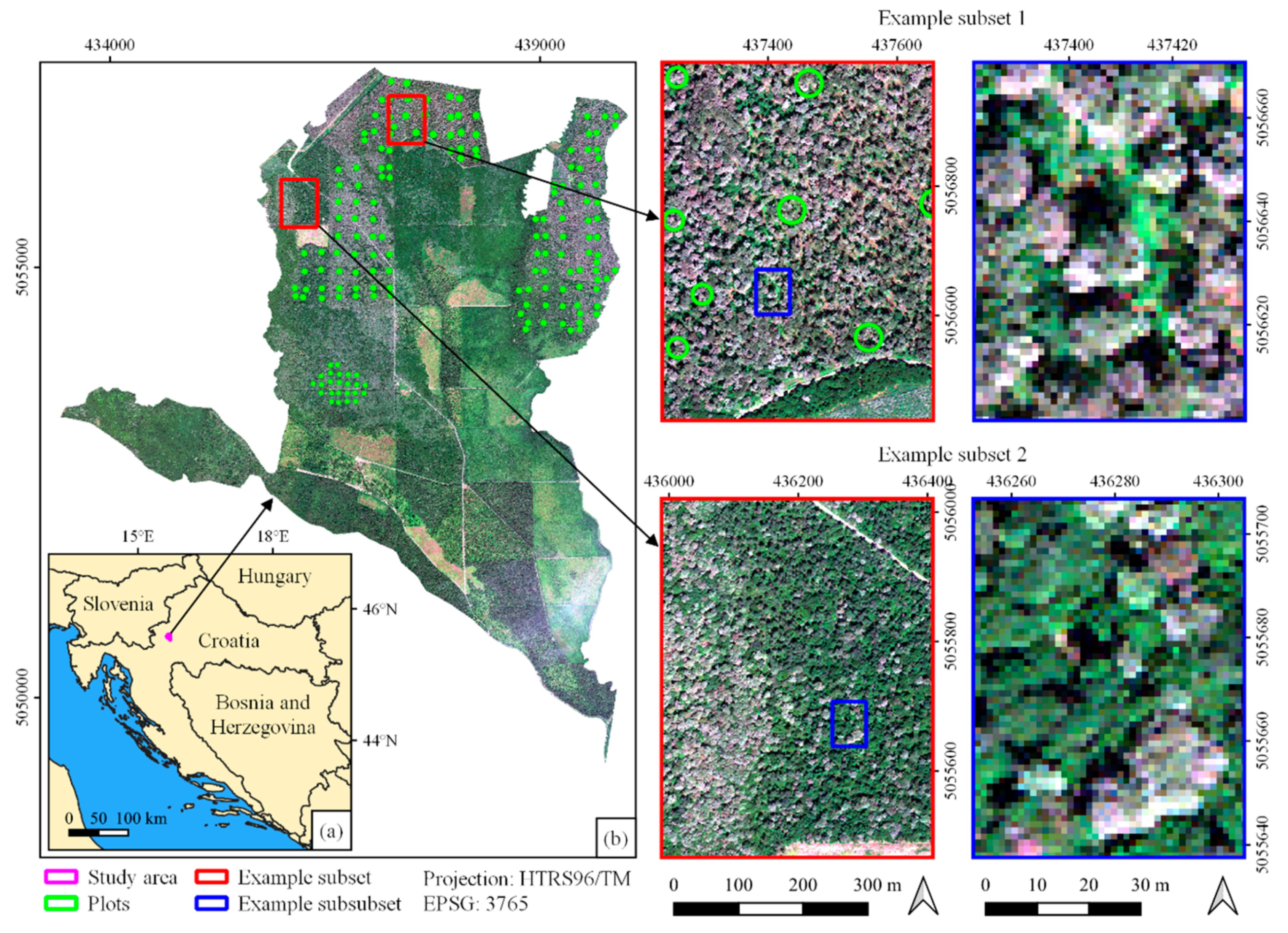
The study area is located in the Jastrebarski lugovi management unit in central Croatia, near the city of Jastrebarsko, 35 km southwest of Zagreb (Figure 1). It covers an area of 2128.77 ha of lowland deciduous forests and is a part of the Pokupsko Basin forest complex (≈12,000 ha). The main forest type (management class) in the study area is even-aged pedunculate oak (Quercus robur L.) forests of different age classes, covering 77% of the study area. The oak stands are commonly mixed with secondary tree species, such as common hornbeam (Carpinus betulus L.), black alder (Alnus glutinosa (L.) Geartn.), and narrow-leaved ash (Fraxinus angustifolia Vahl.). Other secondary tree species that occur sporadically throughout the study area are European white elm (Ulmus laevis Pall.), silver (white) birch (Betula pendula Roth.), lime (Tilia sp.), and poplars (Populus sp.). In addition to oak management class, two other forest types present in the study area are even-aged narrow-leaved ash and even-aged common hornbeam management classes, covering 17% and 6% of the study area, respectively. Unlike the oak stands, ash and hornbeam stands are more homogeneous and less mixed with secondary tree species. The forests of the study area are state-owned, and they are actively managed for sustained timber based on 140- (oak stands), 80- (ash stands), and 70-year (hornbeam stands) rotation cycles, with two or three regeneration fellings during the last 10 years of the rotation. The terrain is mostly flat with ground elevations ranging from 105 to 118 m above sea level (a.s.l.).
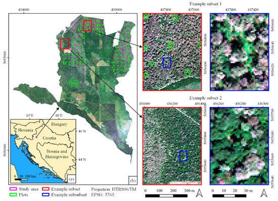
Figure 1.
(a) Location of the study area in Croatia and (b) the study area with two example subset locations (red squares) and sublocations (blue squares) for visual assessment (background: true-color composite of WorldView-3 imagery bands: red-green-blue).
2.2. Field Data
Field data (tree species and tree locations) were collected from a total of 164 circular samples between March and June 2017. Sample plots were systematically distributed (100 × 100 m, 100 m × 200 m, 200 × 100 m, and 200 × 200 m) throughout the 30 stands (subcompartments) within the study area. Of 164 sampled plots, 156 plots were located in 28 oak stands of different ages ranging from 33 to 163 years, while 8 plots were located in two 78-year-old ash stands. The sample plots had radii of 8, 15, or 20 m depending on stand age and stand density. To obtain the precisely measured locations of the plot centers, the Global Navigation Satellite System Real-Time Kinematic (GNSS RTK) method was applied using the Stonex S9IIIN receiver (Stonex, Milan, Italy) connected to the Croatian network of GNSS reference stations [26,27]. The plot centers were measured during leaf-off conditions in the beginning of March 2017. The applied method and service provided fixed solutions for 53 plot centers with an average positioning precision (standard deviation reported by the receiver) of 0.038 m; for 111 plot centers, float solutions were obtained with an average positioning precision of 0.155 m. Within each plot, tree species were determined and recorded, and tree positions were measured for all trees with a diameter at breast height (dbh) above 10 cm. The position of each tree in the plot was recorded by measuring the distance and azimuth from plot center to each tree using a Vertex III hypsometer (Haglöf, Långsele, Sweden) and Haglöf compass (Haglöf, Långsele, Sweden), respectively. In total, species were recorded and positions were measured for 4953 trees within the 164 sample plots. Tree density in sampled plots ranged from 56 to 1840 trees·ha−1, with an average of 526 trees·ha−1 and standard deviation (SD) of 303 trees·ha−1. Table 1 shows the summary statistics of tree density at the plot level for the entire set of 164 field sample plots and for the plots grouped into age classes. Sample plots were not equally distributed across the different age classes due to the irregular distribution of age classes in the study area.

Table 1.
Summary statistics (mean; Min, minimum; Max, maximum; and SD, standard deviation) of tree density (trees·ha−1) at the plot level for the entire set of 164 field sample plots and for the plots grouped into age classes.
2.3. WorldView-3 Satellite Imagery
The WV-3 multispectral imagery used in this study was acquired over the study area in June 2017 with a 2-m spatial resolution at a mean off nadir view angle of 29.2°; with mean in-track and cross-track view angles of −29.2° and −0.5°, respectively; and with mean Sun azimuth and Sun elevation angle of 158.6° and 66.6°, respectively. The WorldView-3 sensor provides eight multispectral bands: coastal blue (B1, 400–450 nm), blue (B2, 450–510 nm), green (B3, 510–580 nm), yellow (B4, 585–625 nm), red (B5, 630–690 nm), red-edge (B6, 705–745 nm), near-infrared 1 (NIR1; B7, 770–895 nm), and near-infrared 2 (NIR2; B8, 860–1040 nm). The satellite also has a panchromatic sensor (Pan, 450–800 nm) that provides imagery with a 0.5-m spatial resolution. However, in this study, only multispectral imagery was used.
3. Methods
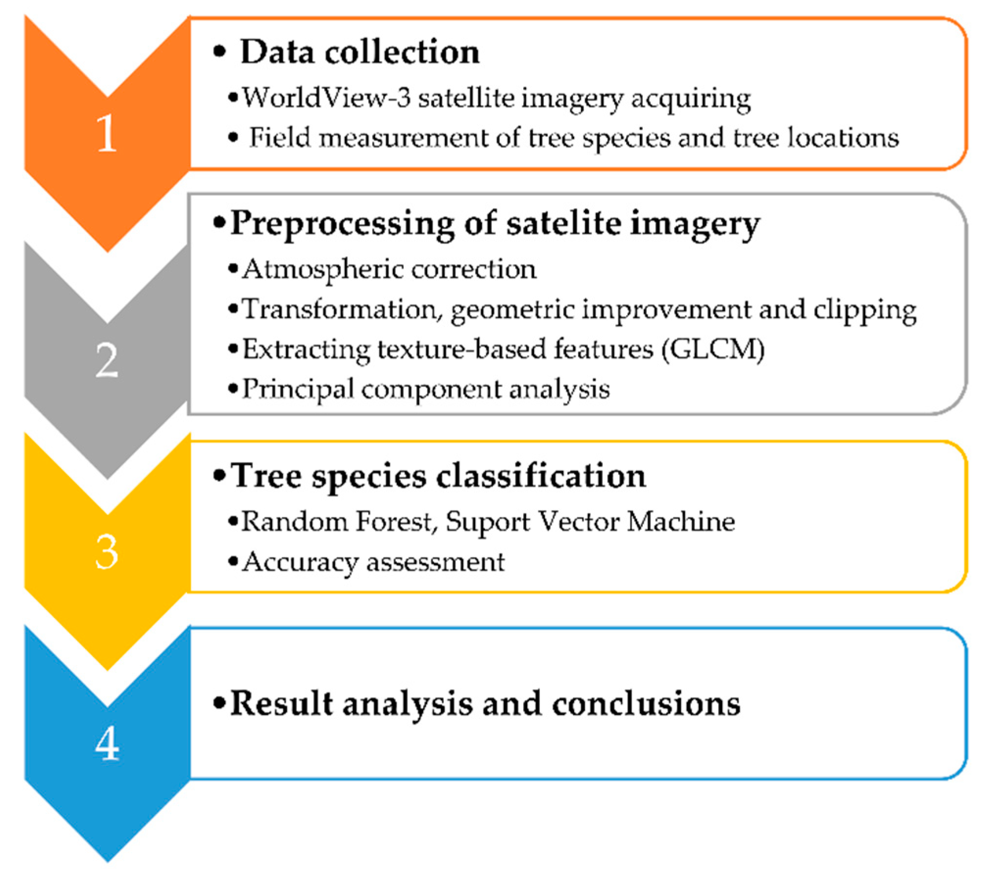
The research workflow in this study was divided into four phases (Figure 2). The entire research was conducted using open source software, e.g., Orfeo ToolBox (6.6.1), Quantum GIS (3.10.1), SAGA GIS (7.0.0), SNAP (7.0.), and Grass GIS (7.8.1).

Figure 2.
Research workflow of tree species classification in mixed deciduous forest using very high spatial resolution satellite imagery and machine learning algorithms.
3.1. Preprocessing of the WorldView-3 Satellite Imagery
To classify tree species using WV-3 imagery, several preprocessing steps were required. As a first step, atmospheric correction was performed. Imagery was transformed into the value of the reflection at the top of the atmosphere (top of atmosphere (TOA) reflectance). Atmospheric correction of the WV-3 satellite imagery was performed according to the second simulation of satellite signal in the solar spectrum (6S) algorithm using the i.atcorr module in GRASS GIS (version 7.8.1.). Based on information about the surface reflectance and atmospheric conditions, this model provides the reflectance of objects at the TOA [28].
Since the field data and satellite imagery did not use the same coordinate system, WV-3 was re-projected from WGS84 UTM 33N to the HTRS96/TM reference coordinate system. The geometric accuracy of WV-3 was improved in two steps: sensor orientation and orthorectification [29]. Sensor orientation was based on rational polynomial coefficients with a shift or zero-order (RPC0) bias correction using seven ground control points (GCPs). The two-dimensional positions of GPCs were recorded using a digital orthophoto map (DOF5), which was an official state map with a scale of 1:5000. Gašparović et al. [30] assessed the accuracy of the digital orthophoto map (DOF5) and WV-2 satellite imagery. The root mean square error (RMSE) for the tested DOF5 ranged between 0.37 and 0.46 m and was more than three times more accurate, on average, compared to orthorectified WV-2 satellite imagery. Since we used MS WV-3 imagery with a 2-m spatial resolution and the accuracy of DOF5 is below 0.5 m, the two-dimensional positions of GPCs recorded from DOF5 have sufficient accuracy. GPCs were acquired in an open-source program, Quantum GIS (QGIS) version 3.10.1, in the HTRS96/TM reference coordinate system. After sensor orientation, WV-3 was orthorectified using a global Shuttle Radar Topography Mission (SRTM) digital elevation model (DEM) with open-source software Orfeo ToolBox (OTB) version 6.6.1. The OTB algorithm for orthorectification was assessed using Monteverdi. Finally, in the last step of preprocessing, satellite imagery was cropped along the border of the Jastrebarski lugovi management unit.
3.2. Visual Interpretation of Reference Polygons for Image Classification
Reference polygons, i.e., polygons used for training and validation of tree species classification, were defined by visual interpretation of WV-3 imagery (B8 = NIR2, B3 = green, and B2 = blue) and by using field data on tree species and tree locations (Figure 3). Due to the complex forest structure in terms of the number of tree species and stand density, visual interpretation of tree species and creation of reference polygons were demanding. Therefore, reference polygons were defined only for the most common tree species (Q. robur, C. betulus, and A. glutinosa) within the field plots as well as for the classes “bare land”, “low vegetation”, and “shadow”. Interpretation was conducted using different imagery compositions for which “true” and “false” color compositions were the most commonly used. One reference polygon mostly contained several neighboring trees of the same species in which crowns were merged or overlapped. A total of 306 reference polygons was collected for tree species, and 67 polygon samples were collected for other classes. All collected reference polygons were randomly divided into training (64%) and validation (36%) datasets (Table 2).
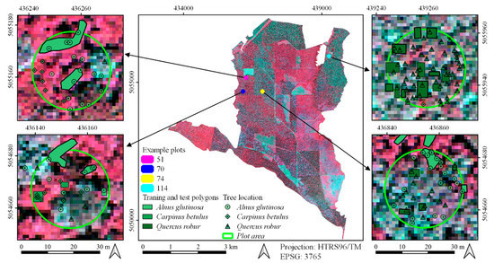
Figure 3.
An example of a visual interpretation of reference polygons on four exemplary field plots (51, 70, 74, and 114) (background: false-color composite of WorldView-3 from 2017, bands: red-green-blue): the measured tree locations from field survey are shown on enlarged maps.

Table 2.
Number of visually interpreted reference polygons (training and validation polygons) for observed tree species and other observed classes (bare land, low vegetation, and shadow).
3.3. Machine Learning Image Classification
In this study, pixel-based supervised image classification was performed using two machine learning algorithms: random forest (RF) and support vector machine (SVM).
RF is an automatic learning algorithm introduced by Breiman [31] and was improved by Adele Cutler [32]. Supervised RF pixel-based classification has been confirmed as useful in separating classes by spectral properties and has therefore been applied in a number of tree species classification studies [13,24,33,34]. RF represents a combination of tree predictors, where each tree depends on the values of a random vector sampled independently. All trees in the forest have the same distribution [31]. The algorithm input is a vector with every single decision tree. The result is a classification label with the most “votes”. The RF classifier uses the Gini index [35]. The Gini index, as an attribute selection criterion, measures the impurity of an attribute in relation to the classes. A comprehensive overview of RF can be found in other studies [31,32,35,36]. To run a RF classifier, open-source software SAGA GIS (7.0.0) was used. Immtzer et al. [33] found that the default values of the Orfeo ToolBox (OTB) parameters for training and classification processes provide optimal results. According to Belgiu and Dragut [36], many studies have investigated the influence of nTree and Mtry parameters on the accuracy of RF classifiers. The most common recommendation, which was applied in this study as well, is to set the nTree parameter to 500 and Mtry to the square root of the number of input variables. In this study, a wide range of values for other parameters were tested, e.g., maximum tree depth of 1 to 1000 and minimum sample count of 1 to 100. Finally, the most accurate results for the RF algorithm were obtained when the maximum depth of the tree was set to 10, while the minimum sample count was set to 2. Regression accuracy was set to 0.01.
Another machine learning algorithm used in this study, the SVM algorithm, was developed by Cortes and Vapnik [37]. In general, SVMs are based on statistical learning theory and define the optimal hyperplane as a linear decision function with a maximal margin between the vectors of two classes. The support vector defines the margin of the largest separation between the two classes. SVM has been shown to be insensitive to high data dimensionality and to be robust in terms of small training sample sizes [38,39]. As in preview studies [17,21,24], the radial basis function (RBF) kernel was used in this study. Cost value and gamma are two user-defined parameters that influence the classification accuracy [40]. Cost value is used to fit the classification errors in the training data set [41] and gamma. The parameters of RBF were set as cost value = 1 and gamma = 0.0001, and probability thresholds were set to zero to avoid unclassified pixels. As well as for RF, to run an SVM classifier, open-source software SAGA GIS (7.0.0) was used.
3.4. Texture Features for Image Classification Improvement
Texture features are one of the important characteristics used for identifying objects from satellite imagery [23]. The most commonly used textural measure is the GLCM [22]. The GLCM is a record of how often different combinations of pixel brightness values (gray levels) occur in imagery [42]. According to Hall-Beyer [42], GLCM features can be categorized into three groups: contrast (contrast, dissimilarity, and homogeneity), orderliness (angular second moment and entropy), and statistics (mean, variance, and correlation). Several studies reported improved classification accuracy when combining GLCM texture and spectral features [43,44]. According to previous research [45,46], to reduce data redundancy, GLCM calculations were performed only for the red channel, which showed the highest entropy among of all bands.
Within this study, we used the GLCM implementation provided with the ESA Sentinel Application Platform SNAP (7.0.). It calculates the 10 Haralick measures: mean, variance, homogeneity, contrast, dissimilarity, energy, entropy, angular second moment, maximum probability, and correlation. Here, we combined the GLCM variance as a measure of the dispersion of the values around the mean with spectral features. The variance was measured according to Equation (1) [42]:
where i is the row number, j is the column number, is the normalized value in the cell i,j, and N is the number of rows or columns. According to Chen et al. [47], who found that for spectrally homogenous classes smaller window sizes improve classification accuracy, GLCM features were computed with a small 5 × 5 pixel window size over all directions, a pixel displacement of 2, and a 32-level quantization.
To extract the most useful texture information from imagery, principal component analysis (PCA) was further applied. PCA is a dimension-reduction technique that can be used to reduce a large set of variables to a small set that still contains most of the information in the original set. PCA finds common factors in a given dataset and ranks them in order of importance [48]. In recent years, PCA has been used extensively in remote sensing classification problems, especially for hyperspectral imagery [49,50,51]. As with GLCM texture extraction, PCA was performed in SNAP (7.0.). The PCA of 10 GLCM measures was performed for WV-3 imagery.
3.5. Accuracy Assessment
For image classification, three different methods were applied and tested in this study:
- Image classification using eight multispectral bands of WV-3 only and RF classifier (RFMS),
- Image classification using eight multispectral bands of WV-3 combined with texture features extracted from WV-3 and the RF classifier (RFMS-GLCM), and
- Image classification using eight multispectral bands of WV-3 combined with texture features extracted from WV-3 and the SVM classifier (SVMMS-GLCM).
The accuracy assessment of image classification and, particularly, the accuracy assessment of tree species classification was conducted using a validation polygon dataset (Table 2).
To evaluate the results of the RF and SVM algorithms, a confusion matrix was produced and the producer’s accuracies (PAs) and user’s accuracies (UAs) for each class were calculated, as were the overall accuracy (OA) [52] and Kappa coefficient (k) [53]. The confusion matrix provided an overview of the classification errors between species. The diagonal represents correctly classified pixels according to reference data, while off-diagonals were misclassified. PA and UA were calculated by dividing the number of correctly classified pixels in each category by the total number of pixels in the corresponding column (PA) or row (UA). OA was computed by dividing the total number of correctly classified pixels by the total number of reference pixels. Besides the OA, within the confusion matrix, omission (O) and commission (C) errors were analyzed.
Developed by Cohen [53], k measures the proportion of agreement after chance agreements were removed from consideration and is calculated using the following equation [53]:
where is the relative observed agreement among raters and is the hypothetical probability of chance agreement. Since the Kappa coefficient has certain limitations identified by Pontius and Millones [54], the figure of merit (FoM) was also calculated as an additional statistical measure (Equation (3)):
where OA represents overall accuracy, O is the number of omissions, and C is the number of commissions.
4. Results
For GLCM texture information extraction, various window sizes were tested (5 × 5, 7 × 7, and 9 × 9). The GLCM feature computed with a 5 × 5-pixel window size produced the best results (as confirmed by Chen et al. [47]), and it was used further in our research. Based on the extracted GLCM features and the conducted PCA, the GLCM variance was confirmed as the most important texture measure, with an eigenvalue considerably greater than that for other GLCM features (Table 3). Therefore, only GLCM variance was included in image classification (RFMS+GLCM and SVMMS+GLCM).

Table 3.
Eigenvalues of principal component analysis (PCA) on 10 gray level cooccurrence matrix (GLCM) texture features.
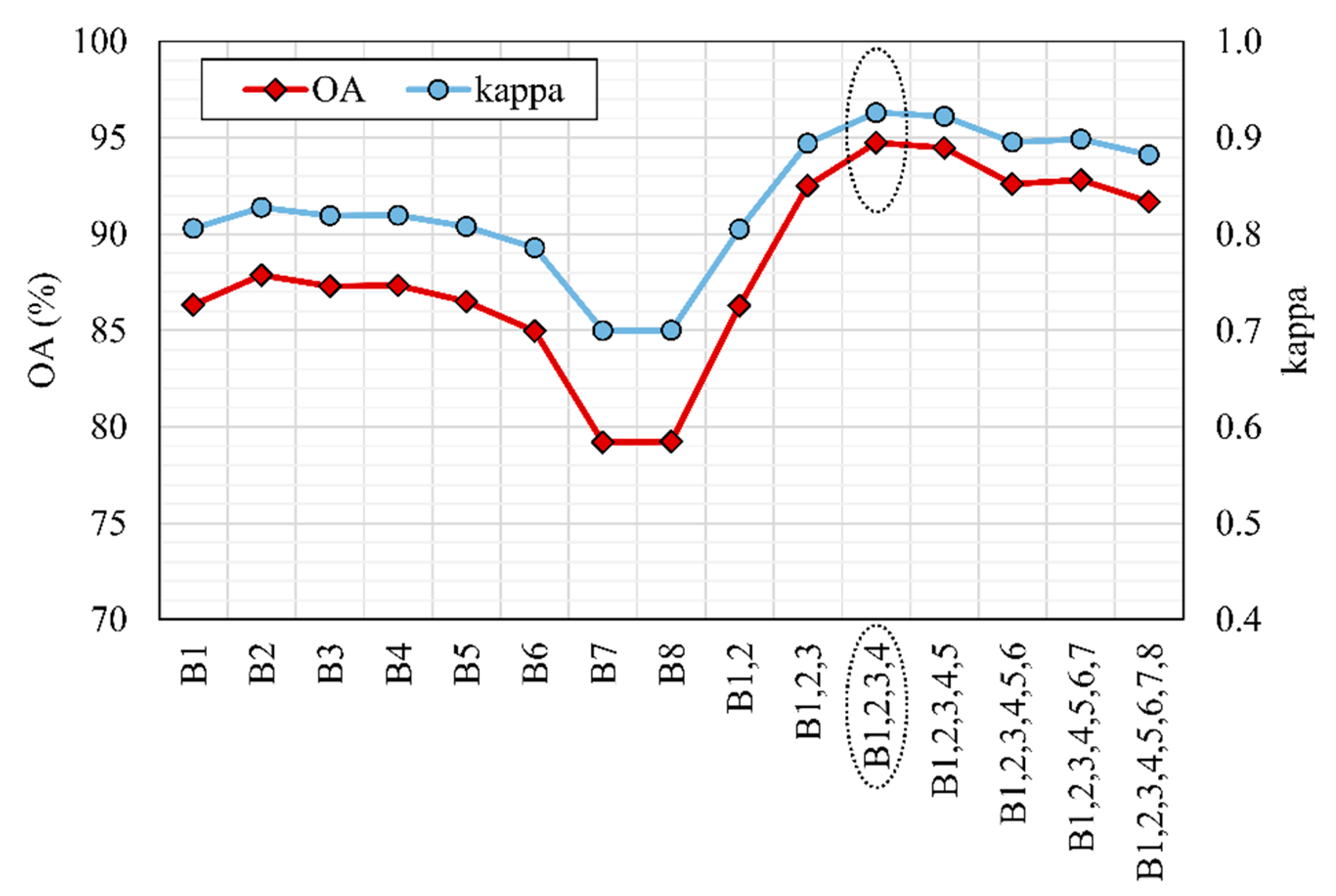
After the most important GLCM feature was determined, the GLCM variance for all eight MS bands was calculated. Prior to tree species classification, additional analysis (experimental classifications) was conducted for the study area to determine for which band or combination of bands GLCM variance provides the best results. In experimental classifications, GLCM variance was calculated for each band separately as well as for different combinations of all eight bands (Figure 4). The obtained results demonstrated that the highest effectiveness of GLCM variance was calculated for the first four bands (B1, B2, B3, and B4). The addition of the GLCM variance of the other bands did not improve the classification accuracy.
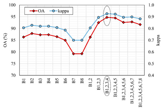
Figure 4.
Overall accuracy (OA) and Kappa values for random forest (RF) experimental classifications based on spectral characteristics of all 8 bands and additional GLCM variance calculated for each band separately as well as for different combinations of bands: labels on the x-axis represent the band or bands for which GLCM variance was calculated, and the dashed oval emphasizes the combination with the highest OA and Kappa value.
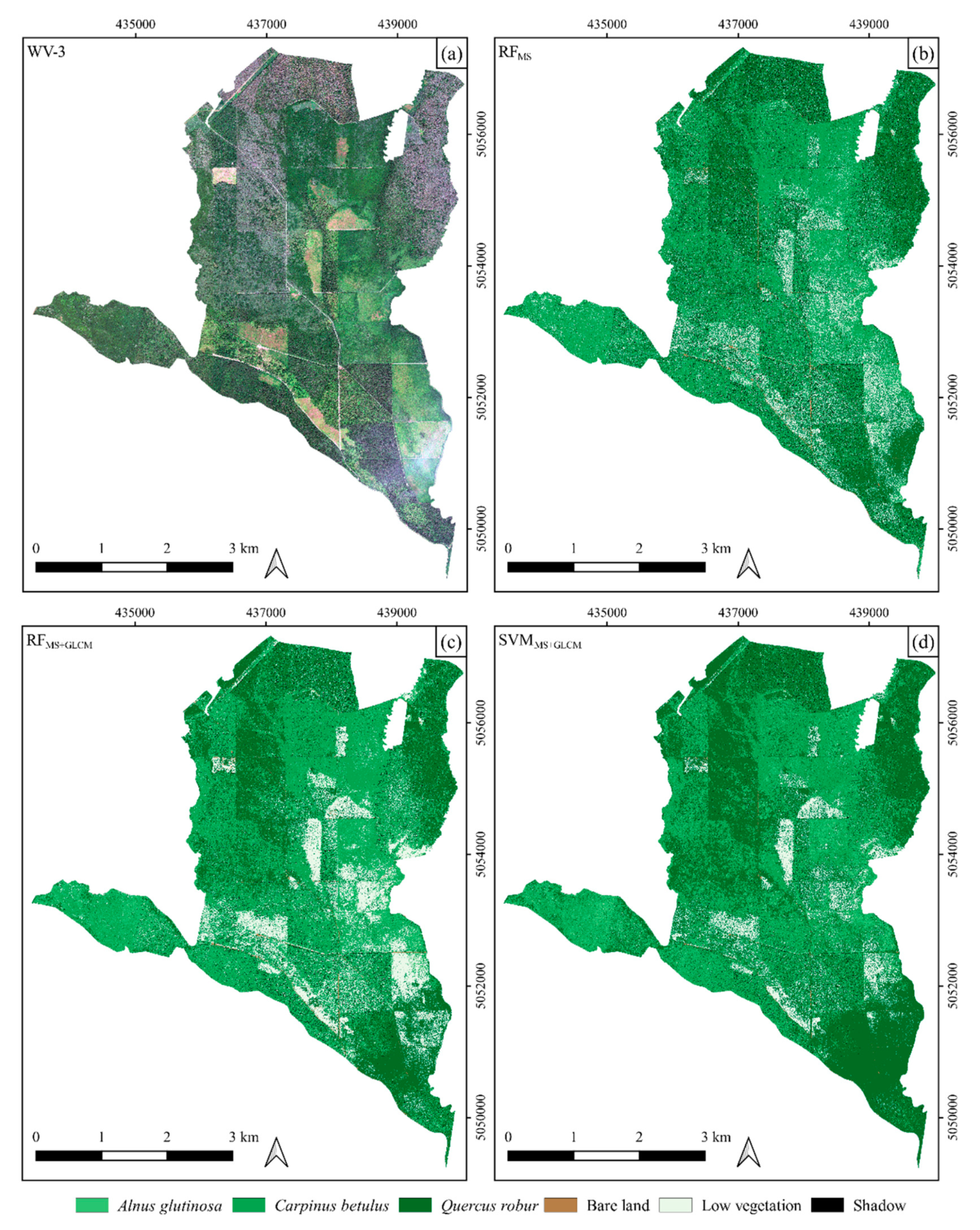
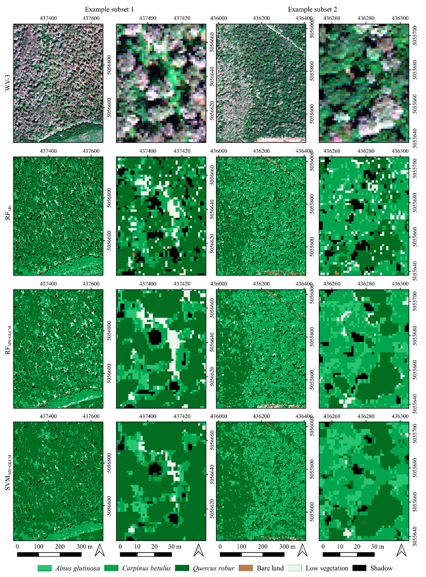
The classification of the WV-3 imagery using three different approaches (RFMS, RFMS-GLCM, and SVMMS-GLCM) and visual analysis of the classification results was conducted for the entire study area; a detailed statistical accuracy assessment was conducted using validation polygons only (Table 2). The results of image classification for the entire study area are shown in Figure 5 (WV-3 true-color composite), whereas Figure 6 presents more detailed classification results for two example subsets.

Figure 5.
Study area shown as WV-3 true-color composite (a) and image classification maps derived by three different approaches: (b) using eight bands of WV-3 imagery and an RF classifier (RFMS); (c) using eight bands of WV-3 combined with texture features extracted from WV-3 imagery and an RF classifier (RFMS+GLCM); and (d) using eight bands of WV-3 combined with texture features extracted from WV-3 and a support vector machine (SVM) classifier (SVMMS+GLCM).
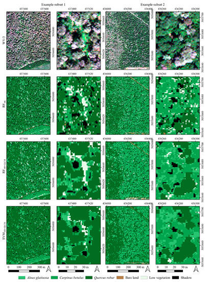
Figure 6.
Two example subsets in the study area: (first row) WV-3 true-color composite; (second row) classification map derived using eight bands of WV-3 imagery and an RF classifier (RFMS); (third row) classification map derived using eight bands of WV-3 combined with texture features extracted from WV-3 imagery and an RF classifier (RFMS+GLCM); and (fourth row) classification map using eight bands of WV-3 combined with texture features extracted from WV-3 imagery and an SVM classifier (SVMMS+GLCM).
An initial visual analysis of the performed classification for the entire study area showed that similar results were obtained using both algorithms (RF and SVM) when eight bands of WV-3 imagery were used in combination with its texture features. This can also be observed in Figure 7, which shows the proportion of observed tree species for the entire study. In other words, the initial visual assessment showed that the RFMS+GLCM and SVMMS+GLCM approaches (methods) provided similar results in automatic classification of mixed deciduous forests for the present study area whereas, when the RFMS approach was applied, i.e., when only multispectral bands of WV-3 imagery were used, different and slightly worse results were obtained. As shown in Figure 5, the classification of WV-3 using only spectral bands (RFMS) produced noisy distribution of tree species classes. This is particularly evident for Alnus glutinosa, which has similar spectral properties to Carpinus betulus.

Figure 7.
The share of observed tree species (Alnus glutinosa, Carpinus betulus, and Quercus robur) for the entire study area obtained with three different approaches (RFMS, RFMS-GLCM, and SVMMS-GLCM).
Besides visual analysis, the classification accuracy was assessed and evaluated using a detailed statistical analysis performed on 136 validation polygons (Table 4). The obtained results showed that, for both algorithms (RF and SVM), the classification accuracy was considerably improved when the texture features (GLCM variance) of WV-3 imagery were considered in addition to the spectral characteristics. Namely, compared to the RFMS classification approach (based solely on WV-3 spectral characteristics), the OA values for RFMS-GLCM and SVMMS-GLCM approaches (both based on WV-3 spectral and texture characteristics) increased by 10% and 7%, respectively. Compared to the RFMS approach, the k values for the RFMS-GLCM and SVMMS-GLCM approaches increased by 0.13 and 0.09, respectively.

Table 4.
Results of accuracy of WV-3 imagery classification using three different approaches (RFMS, RFMS-GLCM, and SVMMS-GLCM) performed on 136 validation polygons. UA, user accuracy; PA, producer accuracy.
Observed by tree species and regardless of the applied classification approach, the lowest classification accuracy was obtained for Alnus glutinosa, with a UA ranging from 43% to 87%. Considerably higher accuracy was obtained for Carpinus betulus (UA = 94–98%), while the highest classification accuracy was obtained for Quercus robur (UA = 97–100%). The classification accuracy for A. glutinosa was considerably improved when the texture feature was added to classification; compared to RFMS approach, the UA values for the RFMS-GLCM and SVMMS-GLCM approaches increased by 40% and 44%, respectively. Slight improvements in classification accuracy were also observed for Q. robur, where UA increased by 2% for RFMS-GLCM and by 3% for the SVMMS-GLCM approach compared to RFMS. Inclusion of the texture feature in classification slightly deteriorated the accuracy for C. betulus compared to the RFMS approach, by 3% and 4% for RFMS-GLCM and SVMMS-GLCM, respectively.
All of the abovementioned were confirmed by an additional accuracy assessment (Table 5) based on FoM, O, C, and A measures. As well as PA and UA, FoM accuracy metrics showed that, for both algorithms (RF and SVM), the classification accuracy was improved by adding texture feature (GLCM variance) to the spectral characteristics.

Table 5.
Additional accuracy assessment of WV-3 imagery classification using three different approaches (RFMS, RFMS-GLCM, and SVMMS-GLCM). FoM, Figure of merit; O, omission; C, commission; A, overall agreement.
5. Discussion
In this study, we evaluated the possibility of tree species classification in a mixed deciduous forest using supervised pixel-based classification of WV-3 satellite imagery with two machine learning algorithms (RF and SVM). Additionally, the contribution of GLCM texture features from WV-3 imagery in tree species classification was evaluated. In general, our findings agree with a number of recent studies [13,15,17,19], which confirmed the potential of very high spatial resolution satellite imagery for tree species classification. However, compared to most of the previous studies conducted in a less complex forest environment [14,18,24,45,55], this research focused on a mixed deciduous forest with pedunculate oak as the main tree species and with large shares of other deciduous tree species. The proportion of tree species varied among the 164 plots distributed within 30 stands of different ages ranging from 33 to 163 years.
Within this study, we evaluated the contribution of 10 GLCM texture features for improvements of tree species classification using PCA. According to Hall-Breyer [56], PCA loadings show that contrast, dissimilarity, entropy, and GLCM variance are generally associated with visual edges of land-cover patches and that homogeneity, GLCM mean, GLCM correlation, and angular second moment are associated with patch interiors. The results obtained in this study confirmed that GLCM variance is the most (and only) important texture feature (Table 3) and, therefore, was the only texture feature included in further analysis.
Window size is an important component of texture analysis. Small windows can increase the differences and can increase the noise content, whereas larger windows cannot effectively extract texture information [57]. Therefore, the effect of window size on classification accuracy was additionally explored by calculating the GLCM with pixel window sizes of 5 × 5, 7 × 7, and 9 × 9. As in Chen et al. [47], the GLCM feature computed with a small 5 × 5 pixel window size produced the most accurate results. In the next step, the GLCM variance that was calculated for each of the eight bands of WV-3 imagery was tested in various combinations (individually for each band or grouped bands) with RF or SVM classifications based on all eight bands (Figure 4). The results showed that GLCM variance calculated for the first four bands (B1, B2, B3, and B4) in combination with the RF or SVM spectral classifications of all eight bands produced the most accurate results.
We also found that, for the applied RF algorithm, the addition of the texture feature (GLCM variance) to the spectral characteristics considerably improved the image classification accuracy (Table 4 and Table 5). The SVM algorithm also produced very accurate results. Almost all accuracy parameters, including FoM, showed improvements for all tree species. These results are in line with other similar studies that also reported an increased overall tree species classification accuracy when spectral and texture features of very high resolution satellite imagery were combined [14,20,21,58,59]. However, the type and number of selected and used texture features differed among studies. For example, eight GLCM texture features (mean, variance, homogeneity, contrast, dissimilarity, entropy, angular second moment, and correlation) were successfully used to improve the species classification in two studies [20,58]. Wang et al. [59] used two texture features (mean, Angular Second Moment (ASM), and entropy) to improve the classification of coastal wetland vegetation from high spatial resolution Pleiades imagery. In several studies that used various remote sensing data for different aims [60,61,62], contrast, entropy, and GLCM mean were chosen as the most contributive texture features to predict forest structural parameters from WV-2 imagery [60], to identify old-growth forests from Sentinel-2 data [61], and to improve the classification in urban areas from SPOT imagery [62]. In this study, GLCM mean and contrast features were the second and third most important variables, respectively, but in comparison to GLCM variance, their contribution to tree species classification accuracy was nonsignificant (Table 3). In contrast to the abovementioned findings and those in this study, Yang et al. [63] reported that GLCM textural features did not improve the classification accuracy of tree species in two observed sites (homogeneous park forest and heterogeneous management forest) in China when combined with spectral features.
In this research, by combining spectral and textural features, the accuracy of tree species classification in mixed deciduous forest was improved for 10% (RF classification approach).
One of the crucial preprocessing steps is the generation of reference polygons. Reference polygons need to fulfill a number of requirements: training and validation polygons must be statistically independent, class-balanced, and representative of the target classes, and the training polygons needs to be large enough to accommodate the increased number of data dimensions [36]. According to Sabat-Tpomala et al. [64], the accuracy of any machine learning procedure is directly related to the quality of the reference polygons used for training and validation of a given classifier. Since, in this study, the research area consisted of natural mixed lowland forest, generation of reference polygons was complex and a time-intensive task. Compared to the other tree species, Alnus glutinosa had the smallest number of reference polygons (Table 2) and, according to the obtained UA and PA values, had the lowest classification accuracy (Table 4). The SVMMS-GLCM approach improved Alnus glutinosa classification accuracy by 4% and 10% in terms of UA and PA, respectively. The SVM algorithm is more resistant to smaller numbers of training patterns compared to the RF algorithm [64].
We demonstrated the potential of both RF and SVM to integrate spectral and textural features for the management of remotely sensed complex data [65,66,67]. Both algorithms classified tree species and other classes within the study area with high accuracy; OAs were 92% and 95% for SVMMS-GLCM and RFMS-GLCM, respectively. Kupidura et al. [67] compared the efficacy of several texture analysis methods as tools for improving land use/land cover classification in satellite imagery and concluded that the choice of the classifier is often less important than adequate data preprocessing to obtain accurate results. Future research will consider other classification algorithms too, especially deep learning convolutional neural networks [68,69,70,71].
6. Conclusions
We confirmed the considerable potential of very high-resolution satellite imagery (WorldView-3) for tree species classification, even in areas with complex, natural, and mixed deciduous forest stands. A total of 373 polygon samples was collected by visual interpretation for six classes (Quercus robur, Carpinus betulus, Alnus glutinosa, bare land, low vegetation, and shadow). Image classification was based on 237 training polygons using pixel-based supervised classification conducted with two machine learning algorithms (RF and SVM). For accuracy assessment, 136 validation polygons were used. The validation results showed the relatively high overall accuracy (85%) for tree species classification based solely on WorldView-3 spectral characteristics and the RF classification approach. As expected, the classification accuracy was improved by a combination of spectral and textural features. With the additional use of GLCM variance calculated for the first four bands, overall accuracy improved by 10% and 7% using the RF and SVM classification approaches, respectively. Principal component analysis confirmed that GLCM variance was the most significant texture feature, whereas additional analysis where GLCM variance was calculated for various combinations of spectral bands demonstrated the greatest effectiveness of GLCM variance when calculated for the first four bands (B1, B2, B3, and B4). The findings of this research should serve as a basis for further studies that should test object-based imagery analysis as well as the influence of the use of pansharpened imagery on the classification accuracy.
Author Contributions
Conceptualization, M.D. and M.G.; methodology, M.D.; software, M.D.; validation, M.D., M.G., and I.B.; formal analysis, M.D. and M.G.; investigation, M.D.; resources, M.D. and M.G.; data curation, M.D., M.G., and I.B.; writing—original draft preparation, M.D.; writing—review and editing, M.D., M.G., and I.B.; visualization, M.D. and M.G.; supervision, M.G. and I.B.; project administration, M.G. and I.B.; funding acquisition, M.G. and I.B. All authors have read and agreed to the published version of the manuscript.
Funding
This research has been supported by projects: Retrieval of Information from Different Optical 3D Remote Sensing Sources for Use in Forest Inventory (3D-FORINVENT), funded by the Croatian Science Foundation (HRZZ IP-2016-06-7686); Operational Sustainable Forestry with Satellite-Based Remote Sensing (MySustainableForest), funded by the European Union’s Horizon 2020 research and innovation program under grant agreement No 776045; and Advanced photogrammetry and remote sensing methods for environmental change monitoring (grant No. RS4ENVIRO), funded by the University of Zagreb.
Conflicts of Interest
The authors declare no conflict of interest.
References
- Gering, L.R.; May, D.M.; Teuber, K.B. The use of aerial photographs and angle-gauge sampling of tree crown diameters for forest inventories. In Proceedings of the State-Of-The-Art Methodology of Forest Inventory, Syracuse, NY, USA, 30 July–5 August 1989; pp. 286–289. [Google Scholar]
- Balenović, I.; Milas, A.S.; Marjanović, H. A Comparison of Stand-Level Volume Estimates from Image-Based Canopy Height Models of Different Spatial Resolutions. Remote Sens. 2017, 9, 205. [Google Scholar] [CrossRef]
- McRoberts, R.E.; Cohen, W.B.; Næsset, E.; Stehman, S.V.; Tomppo, E.O. Using remotely sensed data to construct and assess forest attribute maps and related spatial products. Scand. J. For. Res. 2010, 25, 340–367. [Google Scholar] [CrossRef]
- Lechner, A.M.; Foody, G.M.; Doreen, S.; Boyd, D.S. Applications in Remote Sensing to Forest Ecology and Management. One Earth 2020, 2, 405–412. [Google Scholar] [CrossRef]
- Fassnacht, F.E.; Latifi, H.; Sterenczak, K.; Modzelewska, A.; Lefsky, M.; Waser, L.T.; Straub, C.; Ghosh, A. Review of studies on tree species classification from remotely sensed data. Remote Sens. Environ. 2016, 186, 64–87. [Google Scholar] [CrossRef]
- Knorn, J.; Rabe, A.; Radeloff, V.C.; Kuemmerle, T.; Kozak, J.; Hostert, P. Land cover mapping of large areas using chain classification of neighboring Landsat satellite images. Remote Sens. Environ. 2009, 113, 957–964. [Google Scholar] [CrossRef]
- Griffiths, P.; Linden, S.; Kuemmerle, T.; Hostert, P. A pixel-based Landsat compositing algorithm for large area land cover mapping. IEEE J. Sel. Top. Appl. Earth Obs. Remote Sens. 2013, 6, 2088–2101. [Google Scholar] [CrossRef]
- Chaves, M.E.D.; Picoli, C.A.M.; Sanches, I.D. Recent Applications of Landsat 8/OLI and Sentinel-2/MSI for Land Use and Land Cover Mapping: A Systematic Review. Remote Sens. 2020, 12, 3062. [Google Scholar] [CrossRef]
- Li, X.; Chen, W.; Cheng, X.; Liao, Y.; Chen, G. Comparison and integration of feature reduction methods for land cover classification with RapidEye imagery. Multimed. Tools Appl. 2017, 76, 23041–23057. [Google Scholar] [CrossRef]
- Mas, J.F.; Lemoine-Rodríguez, R.; González-López, R.; López-Sánchez, J.; Piña-Garduño, A.; Herrera-Flores, E. Land use/land cover change detection combining automatic processing and visual interpretation. Eur. J. Remote Sens. 2017, 50, 626–635. [Google Scholar] [CrossRef]
- Nampak, H.; Pradhan, B.; Rizeei, H.M.; Park, H.J. Assessment of land cover and land use change impact on soil loss in a tropical catchment by using multitemporal SPOT-5 satellite images and Revised Universal Soil Loss Equation model. Land Degrad. Dev. 2018, 29, 3440–3455. [Google Scholar] [CrossRef]
- Saini, R.; Ghosh, S.K. Analyzing the impact of red-edge band on land use land cover classification using multispectral RapidEye imagery and machine learning techniques. J. Appl. Remote Sens. 2019, 13, 044511. [Google Scholar] [CrossRef]
- Immitzer, M.; Atzberger, C.; Koukal, T. Tree Species Classification with Random Forest Using Very High Spatial Resolution 8-Band WorldView-2 Satellite Data. Remote Sens. 2012, 4, 2661–2693. [Google Scholar] [CrossRef]
- Ghosh, A.; Joshi, P.K. A comparison of selected classification algorithms for mapping bamboo patches in lower Gangetic plains using very high resolution WorldView 2 imagery. Int. J. Appl. Earth Obs. Geoinf. 2014, 26, 298–311. [Google Scholar] [CrossRef]
- Peerbhay, K.Y.; Mutanga, O.; Ismail, R. Investigating the capability of few strategically placed WorldView-2 multispectral bands to discriminate forest species in KwaZulu-Natal, South Africa. IEEE J. Sel. Top. Appl. Earth Obs. Remote Sens. 2013, 7, 307–316. [Google Scholar] [CrossRef]
- Cho, M.A.; Malahlela, O.; Ramoelo, A. Assessing the utility worldview-2 imagery for tree species mapping in south african subtropical humid forest and the conservation implications: Dukuduku forest patch as case study. Int. J. Appl. Earth Obs. Geoinf. 2015, 38, 349–357. [Google Scholar] [CrossRef]
- Omer, G.; Mutanga, O.; Abdel-Rahman, E.M.; Adam, E. Performance of Support Vector Machines and Artificial Neural Network for Mapping Endangered Tree Species Using WorldView-2 Data in Dukuduku Forest, South Africa. IEEE J. Sel. Top. Appl. Earth Obs. Remote Sens. 2015, 8, 4825–4840. [Google Scholar] [CrossRef]
- Karlson, M.; Ostwald, M.; Reese, H.; Roméo, B.; Boalidioa, T. Assessing the potential of multi-seasonal WorldView-2 imagery for mapping West African agroforestry tree species. Int. J. Appl. Earth Obs. Geoinf. 2016, 50, 80–88. [Google Scholar] [CrossRef]
- Waser, L.T.; Küchler, M.; Jütte, K.; Stampfer, T. Evaluating the Potential of WorldView-2 Data to Classify Tree Species and Different Levels of Ash Mortality. Remote Sens. 2014, 6, 4515–4545. [Google Scholar] [CrossRef]
- Ferreira, M.P.; Wagner, F.H.; Aragão, L.E.; Shimabukuro, Y.E.; de Souza, C.R.F. Tree species classification in tropical forests using visible to shortwave infrared WorldView-3 images and texture analysis. ISPRS J. Photogramm. Remote Sens. 2019, 149, 119–131. [Google Scholar] [CrossRef]
- Xie, Z.; Chen, Y.; Lu, D.; Li, G.; Chen, E. Classification of Land Cover, Forest, and Tree Species Classes with ZiYuan-3 Multispectral and Stereo Data. Remote Sens. 2019, 11, 164. [Google Scholar] [CrossRef]
- Haralick, R.M. Statistical and structural approaches to texture. Proc. IEEE 1979, 67, 786–804. [Google Scholar] [CrossRef]
- Gašparović, M.; Dobrinić, D. Comparative Assessment of Machine Learning Methods for Urban Vegetation Mapping Using Multitemporal Sentinel-1 Imagery. Remote Sens. 2020, 12, 1952. [Google Scholar] [CrossRef]
- Li, D.; Ke, Y.; Gong, H.; Li, X. Object-Based Urban Tree Species Classification Using Bi-Temporal WorldView-2 and WorldView-3 Images. Remote Sens. 2015, 7, 16917–16937. [Google Scholar] [CrossRef]
- Majid, I.A.; Latif, Z.A.; Adnan, N.A. Tree Species Classification Using WorldView-3 Data. In Proceedings of the IEEE 7th Control and System Graduate Research Colloquium, Shah Alam, Malaysia, 8 August 2016; pp. 73–76. [Google Scholar]
- Dragčević, D.; Pavasović, M.; Bašić, T. Accuracy validation of official Croatian geoid solutions over the area of City of Zagreb. Geofizika 2016, 33, 183–206. [Google Scholar] [CrossRef]
- Jurjević, L.; Gašparović, M.; Milas, A.S.; Balenović, I. Impact of UAS Image Orientation on Accuracy of Forest Inventory Attributes. Remote Sens. 2020, 12, 404. [Google Scholar] [CrossRef]
- Vermote, E.F.; Tanre, D.; Deuze, J.L.; Herman, M.; Morcrette, J.J. Second simulation of the satellite signal in the solar spectrum, 6S: An overview. IEEE Trans. Geosci. Remote Sens. 1997, 35, 675–686. [Google Scholar] [CrossRef]
- Gašparović, M.; Dobrinić, D.; Medak, D. Geometric accuracy improvement of WorldView-2 imagery using freely available DEM data. Photogramm. Rec. 2019, 34, 266–281. [Google Scholar] [CrossRef]
- Gašparović, M.; Dobrinić, D.; Medak, D. Spatial accuracy analysis of aerial and satellite imagery of Zagreb. Geodetski List. 2018, 72, 1–14. [Google Scholar]
- Breiman, L. Random Forests. Mach. Learn. 2001, 45, 5–32. [Google Scholar] [CrossRef]
- Cutler, D.R.; Edwards, T.C.; Beard, K.H.; Cutler, A.; Hess, K.T.; Gibson, J.; Lawler, J.J. Random Forests For Classification In Ecology. Ecology 2007, 88, 2783–2792. [Google Scholar] [CrossRef]
- Immitzer, M.; Vuolo, F.; Atzberger, C. First Experience with Sentinel-2 Data for Crop and Tree Species Classifications in Central Europe. Remote Sens. 2016, 8, 166. [Google Scholar] [CrossRef]
- Huesca, M.; Roth, K.L.; García, M.; Ustin, S.L. Discrimination of Canopy Structural Types in the Sierra Nevada Mountains in Central California. Remote Sens. 2019, 11, 1100. [Google Scholar] [CrossRef]
- Pal, M. Random forest classifier for remote sensing classification. Int. J. Remote Sens. 2005, 26, 217–222. [Google Scholar] [CrossRef]
- Belgiu, M.; Drăguţ, L. Random forest in remote sensing: A review of applications and future directions. ISPRS J. Photogramm. Remote Sens. 2016, 114, 24–31. [Google Scholar] [CrossRef]
- Cortes, C.; Vapnik, V. Support vector network. Mach. Learn. 1995, 3, 273–297. [Google Scholar] [CrossRef]
- Van der Linden, S. Classifying segmented hyperspectral data from a heterogeneous urban environment using support vector machines. J. Appl. Remote Sens. 2007, 1, 013543. [Google Scholar] [CrossRef]
- Brown, M.; Gunn, S.R.; Lewis, H.G. Support vector machines for optimal classification and spectral unmixing. Ecol. Model. 1999, 120, 167–179. [Google Scholar] [CrossRef]
- Burges, C.J. A tutorial on support vector machines for pattern recognition. Data Min. Knowl. Discov. 1998, 2, 121–167. [Google Scholar] [CrossRef]
- Adam, E.; Mutanga, O.; Odindi, J.; Abdel-Rahman, E.M. Land-use/cover classification in a heterogeneous coastal landscape using RapidEye imagery: Evaluating the performance of random forest and support vector machines classifiers. Int. J. Remote Sens. 2014, 35, 3440–3458. [Google Scholar] [CrossRef]
- Hall-Beyer, M. GLCM Texture: A Tutorial v. 3.0 March 2017; University of Calgary: Calgary, Canada, 2017. [Google Scholar]
- Johansen, K.; Phinn, S. Mapping Structural Parameters and Species Composition of Riparian Vegetation Using IKONOS and Landsat ETM+ Data in Australian Tropical Savannahs. Photogramm. Eng. Remote Sens. 2006, 72, 71–80. [Google Scholar] [CrossRef]
- Mallinis, G.; Koutsias, N.; Tsakiri, M.; Karteris, M. Object-based classification using Quickbird imagery for delineating forest vegetation polygons in a Mediterranean test site. ISPRS J. Photogramm. Remote Sens. 2008, 63, 237–250. [Google Scholar] [CrossRef]
- Pu, R.; Landry, S. A comparative analysis of high spatial resolution IKONOS and WorldView-2 imagery for mapping urban tree species. Remote Sens. Environ. 2012, 124, 516–533. [Google Scholar] [CrossRef]
- Dorigo, W.; Lucieer, A.; Podobnikar, T.; Carni, A. Mapping invasive Fallopia japonica by combined spectral, spatial, and temporal analysis of digital orthophotos. Int. J. Appl. Earth Obs. Geoinf. 2012, 19, 185–195. [Google Scholar] [CrossRef]
- Chen, D.; Stow, D.A.; Gong, P. Examining the effect of spatial resolution and texture window size on classification accuracy: An urban environment case. Int. J. Remote Sens. 2004, 25, 2177–2192. [Google Scholar] [CrossRef]
- Snap Documentation. Available online: https://docs-snaplogic.atlassian.net/wiki/home (accessed on 7 May 2020).
- Lee, J.; Cai, X.; Lellmann, J.; Dalponte, M.; Malhi, Y.; Butt, N.; Morecroft, M.; Schönlieb, C.B.; Coomes, D. Individual Tree Species Classification From Airborne Multisensor Imagery Using Robust PCA. IEEE J. Sel. Top. Appl. Earth Obs. Remote Sens. 2016, 9, 2554–2567. [Google Scholar] [CrossRef]
- Deng, J.S.; Wang, K.; Deng, Y.H.; Qi, G.J. PCA-based land-use change detection and analysis using multitemporal and multisensor satellite data. Int. J. Remote Sens. 2008, 29, 4823–4838. [Google Scholar] [CrossRef]
- Knauer, U.; von Rekowski, C.S.; Stecklina, M.; Krokotsch, T.; Pham Minh, T.; Hauffe, V.; Kilias, D.; Ehrhardt, I.; Sagischewski, H.; Chmara, S.; et al. Tree Species Classification Based on Hybrid Ensembles of a Convolutional Neural Network (CNN) and Random Forest Classifiers. Remote Sens. 2019, 11, 2788. [Google Scholar] [CrossRef]
- Congalton, R.G. A review of assessing the accuracy of classifications of remotely sensed data. Remote Sens. Environ. 1991, 37, 35–46. [Google Scholar] [CrossRef]
- Cohen, J. A Coefficient of Agreement for Nominal Scales. Educ. Psychol. Meas. 1960, 20, 37–46. [Google Scholar] [CrossRef]
- Pontius, R.G.; Millones, M. Death to Kappa: Birth of quantity disagreement and allocation disagreement for accuracy assessment. Int. J. Remote Sens. 2011, 32, 4407–4429. [Google Scholar] [CrossRef]
- Gebreslasie, M.T.; Ahmed, F.B.; van Aardt, J.A.N. Extracting structural attributes from IKONOS imagery for Eucalyptus plantation forests in KwaZulu-Natal, South Africa, using image texture analysis and artificial neural networks. Int. J. Remote Sens. 2011, 32, 7677–7701. [Google Scholar] [CrossRef]
- Hall-Beyer, M. Practical guidelines for choosing GLCM textures to use in landscape classification tasks over a range of moderate spatial scales. Int. J. Remote Sens. 2017, 38, 1312–1338. [Google Scholar] [CrossRef]
- Attarchi, S.; Gloaguen, R. Classifying Complex Mountainous Forests with L-Band SAR and Landsat Data Integration: A Comparison among Different Machine Learning Methods in the Hyrcanian Forest. Remote Sens. 2014, 6, 3624–3647. [Google Scholar] [CrossRef]
- Wang, H.; Zhao, Y.; Pu, R.; Zhang, Z. Mapping Robinia Pseudoacacia Forest Health Conditions by Using Combined Spectral, Spatial, and Textural Information Extracted from IKONOS Imagery and Random Forest Classifier. Remote Sens. 2015, 7, 9020–9044. [Google Scholar] [CrossRef]
- Wang, M.; Fei, X.; Zhang, Y.; Chen, Z.; Wang, X.; Tsou, J.Y.; Liu, D.; Lu, X. Assessing Texture Features to Classify Coastal Wetland Vegetation from High Spatial Resolution Imagery Using Completed Local Binary Patterns (CLBP). Remote Sens. 2018, 10, 778. [Google Scholar] [CrossRef]
- Ozdemir, I.; Karnieli, A. Predicting forest structural parameters using the image texture derived from WorldView-2 multispectral imagery in a dryland forest, Israel. Int. J. Appl. Earth Obs. Geoinf. 2011, 13, 701–710. [Google Scholar] [CrossRef]
- Spracklen, B.D.; Spracklen, D.V. Identifying European Old-Growth Forests using Remote Sensing: A Study in the Ukrainian Carpathians. Forests 2019, 10, 127. [Google Scholar] [CrossRef]
- Shaban, M.A.; Dikshit, O. Improvement of classification in urban areas by the use of textural features: The case study of Lucknow city, Uttar Pradesh. Int. J. Remote Sens. 2001, 22, 565–593. [Google Scholar] [CrossRef]
- Yang, G.; Zhao, Y.; Li, B.; Ma, Y.; Li, R.; Jing, J.; Dian, Y. Tree Species Classification by Employing Multiple Features Acquired from Integrated Sensors. J. Sens. 2019, 2019, 1–12. [Google Scholar] [CrossRef]
- Sabat-Tomala, A.; Raczko, E.; Zagajewski, B. Comparison of Support Vector Machine and Random Forest Algorithms for Invasive and Expansive Species Classification Using Airborne Hyperspectral Data. Remote Sens. 2020, 12, 516. [Google Scholar] [CrossRef]
- Dye, M.; Mutanga, O.; Ismail, R. Combining spectral and textural remote sensing variables using the random forest ensemble: Predicting the age of Pinus patula forests in KwaZulu-Natal, South Africa. Spat. Sci. 2012, 57, 197–215. [Google Scholar]
- Zhang, L.; Liu, Z.; Ren, T.; Liu, D.; Ma, Z.; Tong, L.; Zhang, C.; Zhou, T.; Zhang, X.; Li, S. Identification of Seed Maize Fields With High Spatial Resolution and Multiple Spectral Remote Sensing Using Random Forest Classifier. Remote Sens. 2020, 12, 362. [Google Scholar] [CrossRef]
- Kupidura, P. The Comparison of Different Methods of Texture Analysis for Their Efficacy for Land Use Classification in Satellite Imagery. Remote Sens. 2019, 11, 1233. [Google Scholar] [CrossRef]
- Nezami, S.; Khoramshahi, E.; Nevalainen, O.; Pölönen, I.; Honkavaara, E. Tree Species Classification of Drone Hyperspectral and RGB Imagery with Deep Learning Convolutional Neural Networks. Remote Sens. 2020, 12, 1070. [Google Scholar] [CrossRef]
- Miyoshi, G.T.; Arruda, M.S.; Osco, L.P.; Junior, J.M.; Gonçalves, D.N.; Imai, N.N.; Tommaselli, A.M.G.; Honkavaara, E.; Gonçalves, W.N. A Novel Deep Learning Method to Identify Single Tree Species in UAV-Based Hyperspectral Images. Remote Sens. 2020, 12, 1294. [Google Scholar] [CrossRef]
- Schiefer, F.; Kattenborn, T.; Frick, A.; Frey, J.; Schall, P.; Koch, B.; Schmidtlein, S. Mapping forest tree species in high resolution UAV-based RGB-imagery by means of convolutional neural networks. ISPRS J. Photogramm. Remote Sens. 2020, 170, 205–215. [Google Scholar] [CrossRef]
- Grinias, I.; Panagiotakis, C.; Tziritas, G. MRF-based Segmentation and Unsupervised Classification for Building and Road Detection in Peri-urban Areas of High-resolution. ISPRS J. Photogramm. Remote Sens. 2016, 122, 145–166. [Google Scholar] [CrossRef]
Publisher’s Note: MDPI stays neutral with regard to jurisdictional claims in published maps and institutional affiliations. |
© 2020 by the authors. Licensee MDPI, Basel, Switzerland. This article is an open access article distributed under the terms and conditions of the Creative Commons Attribution (CC BY) license (http://creativecommons.org/licenses/by/4.0/).

