Article

Combining SfM Photogrammetry and Terrestrial Laser Scanning to Assess Event-Scale Sediment Budgets along a Gravel-Bed Ephemeral Stream

by
Carmelo Conesa-García
1,*,
Carlos Puig-Mengual
2,
Adrián Riquelme
3,
Roberto Tomás
3,
Francisco Martínez-Capel
2,
Rafael García-Lorenzo
1,
José L. Pastor
3,
Pedro Pérez-Cutillas
1 and
Miguel Cano Gonzalez
3
1
Department of Physical Geography, University of Murcia, 30001 Murcia, Spain
2
Institut d’Investigació per a la Gestió Integrada de Zones Costaneres (IGIC), Universitat Politècnica de València (UPV), 46730 Gandia, Spain
3
Department of Civil Engineering, University of Alicante, 03080 Alicante, Spain
*
Author to whom correspondence should be addressed.
Remote Sens. 2020, 12(21), 3624; https://doi.org/10.3390/rs12213624
Submission received: 16 October 2020 / Revised: 28 October 2020 / Accepted: 30 October 2020 / Published: 4 November 2020
(This article belongs to the Special Issue Quantifying Landscape Evolution and Erosion by Remote Sensing)

Abstract

:
Stream power represents the rate of energy expenditure along a stream reach and can be calculated using topographic data acquired via structure-from-motion (SfM) photogrammetry and terrestrial laser scanning (TLS). This study sought to quantitatively relate morphological adjustments in the Azohía Rambla, a gravel-bed ephemeral stream in southeastern Spain, to stream power (ω), critical power (ωc), and energy gradients (∂ω/∂s), along different reference channel reaches of 200 to 300 m in length. High-resolution digital terrain models (HRDTMs), combined with ortophotographs and point clouds from 2018, 2019, and 2020, and ground-based surveys, were used to estimate the spatial variability of morphological sediment budgets and to assess channel bed mobility during the study period at different spatial scales: reference channel reaches (RCRs), pilot bed survey areas (PBSAs), and representative geomorphic units (RGUs). The optimized complementary role of the SfM technique and terrestrial laser scanning allowed the generation of accurate and reliable HRDTMs, upon which a 1-D hydrodynamic model was calibrated and sediment budgets calculated. The resulting high-resolution maps allowed a spatially explicit analysis of stream power and transport efficiency in relation to volumes of erosion and deposition in the RCR and PBSA. In addition, net incision or downcutting and vertical sedimentary accretion were monitored for each flood event in relation to bedforms and hydraulic variables. Sediment sources and sinks and bed armoring processes showed different trends according to the critical energy and stream power gradient, which were verified from field observations. During flows exceeding bankfull discharges (between 18 and 24 m3 s−1 according to channel reach), significant variations in ∂ω/∂s values and ω/ωc ratios (e.g., −15 < ∂ω/∂s < 15 Wm−3; ω/ωc > 2 for a peak discharge of 31 m3 s−1) were associated with a large amount of bedload mobilized upstream and vertical accretion along the middle reach (average rise height of 0.20 to 0.35 m for the same event). By contrast, more moderate peak flows (≤10 m3 s−1) only produced minor changes resulting in surface washing, selective transport, and local bed scouring.

Graphical Abstract

1. Introduction

Ephemeral streams are dry, irregular, and often unpredictable watercourses, particularly sensitive to short-term climatic changes and to human impacts. Consequently, their response can be highly variable, ranging from slight river-bed adjustments [1] to overall changes in channel geometry after flash floods [2,3,4]. This type of stream is found in large areas around the world, in arid and semi-arid environments, where quite fragile hydromorphological systems often form, subjected to a metastable dynamic equilibrium that strongly depends on the frequency and magnitude of floods. During periods of relatively more frequent and lower magnitude peak flows, surface bed washing and downcutting phenomena can produce secondary channels, lateral erosion, and partial destruction of low bars [5]. Infrequent and large floods affect the entire main channel, modifying its global geometry, and create prominent features of aggradation and incision, depending on the bed materials [2].
Although ephemeral streams tend to maintain similar flow characteristics over long periods of time [6], there are semi-arid Mediterranean areas whose dry and intermittent streams are being subjected to the effects of the current climate change and have begun to show signs of relatively rapid geomorphic adjustment. A clear example of this is the coastal drainage system in southeastern Spain, mainly composed of ephemeral gravel-bed streams. These ephemeral channels usually transport a high tractive load from heavily weathered headwater areas and alluvial channel banks, producing an abundant amount of coarse sediment (gravel and pebbles). In general, they are channels with a high width-to-depth ratio, which, except in sections of structural geological control, run through poorly consolidated alluvial formations, showing great dynamism and instability. Their upper reaches dissect steep alluvial fans, giving rise to entrenched and deep channels subjected to downcutting and basal erosion, which cause frequent breaks and collapses of material. In addition, downstream, these gravel-bed streams experience channel widening, aggradation, and bed armoring [7]. As a result, the streambed often is very permeable, so flood peak discharges decrease sharply downstream due to transmission losses [8,9]. Due to high infiltration rates, incision, and transport capacity decrease, while vegetation tends to grow locally on stable bars and subsurface moisture storage increases, promoting positive feedback for instream aggradation [10,11,12]. Downstream, alluvium within the channel increases in thickness and smooths the bed slope, creating a channel profile that is straighter than concave, unlike in perennial rivers [13,14].
The scientific literature on spatial morphological variability in this type of ephemeral streams in relation to erosion volumes, deposition, and sediment transport (sediment budget) on a detailed scale is scarce. Recently, high-resolution techniques, such as structure-from-motion (SfM) photogrammetry and terrestrial laser scanning (TLS), have been tested to evaluate morphological adjustments in ephemeral streams [15,16,17,18,19].
In this paper, we propose an approach to assess the event-scale sediment budget along an ephemeral gravel-bed channel that couples the results of the structure-from-motion multi-view stereo (SfM-MVS) and TLS techniques. The use of SfM-MVS in a low-altitude unmanned aerial vehicle (UAV) allows the development of orthomosaics and high-resolution digital elevation models (<5 cm per pixel) [20,21]. This survey product offers significantly better resolution and much lower processing costs than others generated by traditional imaging platforms, such as satellites or aircraft [22,23,24,25]. In geomorphological studies, UAV technology has already been applied to monitor fluvial system changes and dynamics [26,27,28]. The high temporal resolution offered by UAV allows assessment of the rapid evolution of river ecosystems. The UAV-SfM technique, when compared to traditional photogrammetry and other topographic surveying approaches (e.g., total station and DGPS), has proven to be particularly effective for the detection of channel morphological changes [29,30,31].
Laser Imaging Detection and Ranging (LiDAR) is a land surveying technique that accurately measures and collects millions of points in a few minutes, providing geometrical information from a scene by precisely measuring the time-of-flight of laser beams. A laser scanner device can be mounted on moving vehicles, such as UAVs or ground-based vehicles (for TLS). The 3-D point cloud (3DPC) datasets obtained from these techniques have usually exploited geometrical features’ identification and extraction, providing unlimited possibilities in geomorphology and, more specifically, in fluvial geomorphology [20,32,33,34].
In order to estimate the morphological sediment budgets in the study of the gravel-bed stream, three analyses were performed using SfM-MVS and TLS, as follows: (1) An analysis of hydraulic variables at the cell scale was performed for the flash floods under study, based on rasterized information from cross-section data and using 1-D hydrodynamic modeling and high-resolution digital terrain models (HRDTMs); (2) erosion and deposition values and net sediment budgets were extracted from datasets of SfM and TLS for periods with different numbers and magnitudes of events; (3) the 3DPC datasets were used to calculate a set of statistical parameters, regarding elevation and volume differences after each event in reference channel reaches (RCRs), pilot bed survey areas (PBSAs), and representative geomorphic units (RGUs).

2. Study Area and Field Surveys

The SfM and TLS surveys were carried out in the Rambla de la Azohía, located in southeastern Spain (Region of Murcia) (Figure 1). The area drained by this ephemeral stream and its tributaries is relatively small (13 km2), to the point that it could be completely covered by a single storm. The climate of the study area presents strong seasonal contrasts, with extreme droughts and monthly potential evapotranspiration values higher than 140 mm in the summer season. These conditions, together with a scarce vegetation cover and very irregular and intense rains, with records above 50 mm/h, often cause large flash floods [35]. This watercourse is part of a littoral hydrological system made up of numerous ephemeral gravel-bed channels, draining directly into the Mediterranean Sea. Steep slopes modeled on metamorphic poorly permeable materials (mainly phyllites, schists, and quartzites), subjected to intense weathering, constitute an important source of sediments and ensure the supply of coarse particles to the channel when heavy rains occur. As a result of this, the Rambla de la Azohía exhibits a particularly active morphodynamics, ranging from minor bed alterations to large morphological channel changes.
Instead of using a monthly or annual time scale, singular extreme hydrological events, isolated in time, were analyzed to determine overall and local morphological channel changes and sediment budgets at different spatial scales: RCR, PBSA, and RGU (Figure 1 and Figure 2). Specifically, morphological changes were monitored in three stages: (1) September 2018 to September 2019, including the events of 18 November 2018 and April 2019 (31.3 m3 s−1) (from SfM data); (2) December 2018 to September 2019, including only the flash flood on 19–20 April 2019 (from TLS data); and (3) September 2019 to January 2020, in which peak flows occurred on 12–13 September 2019 (10.9 m3 s−1) and 2 December 2019 (from TLS data). Only the April event exceeded the bankfull discharge and locally affected the active flood area in non-entrenched cross-sections.
The first two flow events of the analysis period (18 November 2018 and 19–20 April 2019) were monitored by UAV and TLS, covering survey areas with different extensions (Figure 2). The UAV-SfM of September 2018 covered a wide area (>600 m in length) along the upper, middle, and lower sections of the study stream, while the TLS only comprised the RCR, upper (UPR) and middle (MDR) shortened reaches (<200 m long), and their respective PBSA within them. After the aforementioned peak flows, a date and common study area were chosen to carry out both SfM-MVS and TLS, in order to obtain the same georeferencing, compare the associated errors, and analyze the possibility of the complementary optimal use in time of both techniques. In fact, the morphological changes produced after the peak flows of 12–13 September and 2 December 2019 were only detected by TLS (Figure 2).

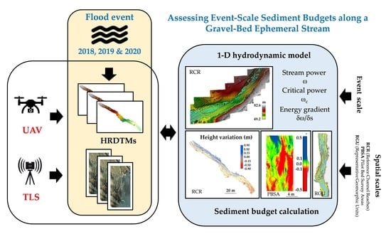
3. Material and Methods

The affected areas, elevation differences, volumes of erosion and deposition, and sediment budgets were obtained for the two RCR (upper (UPR) and middle (MDR) stretches), using data derived from UAV-SfM and TLS. To detect changes in bedload budgets at the bed level exclusively, an analysis was performed using TLS in pilot survey bed areas (PSBAs) with higher point density. The RCRs were delineated using the limits of the water sheet generated by the hydraulic model for each flood event. In addition, the values of the total area of interest (m2), total volume difference average (m3), net thickness difference (m) for the area of interest, and percent imbalance (departure from equilibrium), among other variables, were provided by both techniques for each RGU.

3.1. SfM-MVS Photogrammetry

The remote information was collected with a Phantom 4 Pro, with a 20 Mpx camera and a 1-inch sensor. The photogrammetric parameters of the flights were set before the development of the first field survey and the inspection of the study area, using the software tool DJI GS Pro© with equivalent values for all the surveys; this procedure ensured optimum comparability among the digital elevation models generated at different sites and on different dates. The average flight height was c. 50 m above ground level, resulting in images with a resolution of c. 1 cm.
Standard targets extracted from Agisoft PhotoScan Pro 1.2.2© (Agisoft, St. Petersburg, Russia) were used as ground control points (GCPs) for georeferencing and analyzing the quality of the reconstructed HRDTM. These targets were randomly distributed throughout each of the stream segments and were surveyed using a Prexiso G5© (Leica, Wetzlar, Germany) GPS-RTK instrument. The GPS-RTK instrument was connected to the regional network of GPS GNSS (Network of Reference Stations in the Autonomous Community of Murcia “Meristemum”) via mobile signal, to obtain differential corrections in real time. In each survey, c. 66% of the measured points were subsequently integrated into the model for georeferencing purposes and the remaining 34% were used as checkpoints for the validation of the HRDTM. Permanent GCPs were also installed, using FENO survey markers in each of the GRSs to define common reference points for all surveys and methodologies. All the GPS points were recorded in the WGS84 global reference system.
We selected images with a high level of overlap (80–90%) to ensure successful subsequent image matching [36]. These images and the coordinates of the GCPs’ were uploaded into structure-from-motion photogrammetry software, Agisoft PhotoScan Pro v.1.2.2© (Agisoft, Russia), and aligned using high-precision settings and generic pair preselection to create a sparse point cloud [37,38]. We optimized the image alignment using the GCPs’ data and regenerated the model using the same settings as previously; consequently, the HRDTM, orthophoto, and dense point cloud were exported for further analysis in a global georeferencing system (WGS84).
The difference between the UAVs-collected HRDTM (DoD) in different field surveys, as well as between the TLS-generated HRDTM, was calculated in ArcGis 10.5 © (ESRI, Redlands, CA, USA), by subtracting the final topography from the previous topography for the same area [17]. The same polygon was used for the comparison of the complete RCR, and similarly for the RGU, to maintain the boundaries for change detection, and the HRDTMs were created with equal pixel size (0.02 × 0.02 m), starting from a specific point, so that the grid cells were fully coincident. To assess the sediment budgets and morphological bed changes, we used statistical data on differences in area, volume, height, and percent imbalance for each of the RGUs. In addition, histograms of the volume and bar graphs were used to represent the trends of elevations.

3.2. Terrestrial Laser Scanning (TLS)

In this study, a terrestrial 3-D laser scanner (Leica ScanStation C10 model) was used. This instrument captures the coordinates of points up to 200 m away and the returned energy, and estimates the RBG color using a digital camera. The precision of the instrument is 2 mm. The TLS captures the evenly spaced points when the surface is vertical, but when it is sub-horizontal, the scanned points are sparse. Consequently, to scan the bedforms, it is necessary to choose elevated positions for the scanner, when possible. Another option is to perform multiple scanning stations and to register them, merging sparse point clouds and reducing the point spacing and the shadow areas.
Several scans were made from different stations placed strategically along the bedforms for detailed geometrical definition using TLS. For each date, several scanning stations were made and registered using HDS targets. In addition, the FENO survey markers were also scanned in order to register the TLS point clouds described in the previous section and the SfM datasets. The scan performed on 5 September 2019 was used as the benchmark for all the TLS scans. On that date, the SfM and TLS data were acquired. The coordinates of the FENO survey markers were extracted from that SfM dataset and the TLS dataset was registered using those coordinates. Consequently, the 2018 and 2020 scans were registered to that benchmark using existing buildings as the reference. The registration was performed using the ICP plugin of CloudCompare [39] and was applied to existing buildings, which were considered as stable areas for the whole study period. Then, the registration was evaluated using the M3C2 plugin of CloudCompare. Both registrations had a mean error of 2 mm.
To study the elevation differences and volume changes, two pilot bed survey areas (PBSAs) with higher point density, within the UPR and MDR reference channel reaches, were selected: the upper area (8.55 × 17.7 m2), and the middle area (16.3 × 27.55 m2). The existing vegetation (scrub, bushes, and trees) was removed using the Canupo (CAractérisation de NUages de POints) CloudCompare plugin with specific trainings for both areas [40] (Figure 3). Then, each area was rasterized using a 5-cm grid and empty areas were interpolated.

3.3. Criteria for the Selection of Reference Channel Reaches (RCRs), Pilot Bed Survey Areas (PBSAs), and Representative Geomorphic Units (RGUs)

Reference upper and middle reaches (upper and middle RCR) were chosen depending on the accessibility and the presence of potentially active surface areas. In addition, these stream stretches better represent the variations in the sediment budget and morphological adjustments within the main channel, as opposed to the lower reach, whose global changes are the product of sediment-laden flood water spills, affecting crevasse splays and a wide active flood bed. In fact, the choice of the upper and middle RCR in this ephemeral gravel-bed stream is intended to reflect the clear influence that coarse grain-sizes and bedload, as the dominant transport modality, have on the morphological sediment budget within the channel itself [41]. Downstream, along the lower reach to the mouth of this stream, a distributary drainage system exists, which implies that the budget of more complex sediments needs to be evaluated, accounting for mixed sources (hillslopes and secondary channels), for the temporary storage of sediment in bars and alluvial plains [42].
The upper RCR is an entrenched channel stretch that enabled one scanning station at an elevated position. The rest of the scans were performed on the ground close to the bedforms. In the middle RCR, where bedforms arises and the vegetation cover is scarce, only scanning stations on the ground were performed, reducing the density of the points. The choice of PBSA is intended to detect and quantify precise changes in bed sediment budgets and bed load mobility, while the RGU monitoring allows us to analyze behavior patterns and spatial variability of forms associated with scouring and deposition areas within the channel.

3.4. Hydrometeorological and Hydraulic Data

A rainfall-runoff model was used to simulate runoff on the basis of rainfall events during the budget period. Five pre-simulated runoff events were defined on the basis of the rainfall amount, initial wetness conditions, and initial discharge and were subsequently adjusted according to the real flow heights measured by water pressure sensors. The HEC-HMS 3.5 program [43] was combined with a DTM in grid format and 4 × 4 m cell resolution [44] in order to generate the drainage patterns and catchment limits. Then, in accordance with [45], we assembled the headwater sub-basins that are homogeneous in texture and roughness and individualized those affected by confluences with important breaks in the bed slope. The main abstraction used was the infiltration curve number (NC) of each sub-basin, following the methodology of the Soil Conservation Service of the US Department of Agriculture [46]. The geometries and data tables, referring to the vector lithological layer of the Geological and Mining Institute of Spain (IGME) at a scale of 1: 50,000, and the land use map of the Corine Land Cover (CLC), Level 3 (2012) were combined using GIS to estimate this parameter, according to the different hydrological soil groups and substrate textures. Using the antecedent conditions of dry soil and pluviometric data for intervals of 5 min at the Cuesta del Cedacero station, we calculated the dimensionless unit hydrograph of the SCS and its peak unit flow (qp) (m3 s−1) (Equation (1)):
q p = 2.08   A T p ,
where A is the area of the basin (km2) and Tp the time to peak (h), estimated according to Equation (2):
T p = D 2 + t p ,
where D is the duration of the effective rainfall (h) and tp is the lag time, in our case, 0.6 times the concentration time of the catchment [47].
The output data (Figure 4) were then transferred to the 1-D hydrodynamic model HEC-RAS [48], supported by HRDTM, to obtain the channel profile and cross-sections and hydraulic variables. A total of 212 cross-sections were used, with an average separation of 2.0–3.5 between them in both channel reaches. The theoretical hydrometeorological discharge, estimated for the conditions of a subcritical flow regime, was calibrated using that from the real water height data. Variations in the water level during each flood event were recorded with levelogger sensors and corrected using barometric calibration devices (barologger sensors), located in a station intermediate between the upper and middle reaches. For all the cross-sections, information concerning the flow surface area, hydraulic radius, velocity, shear stress, and stream power was obtained. The power per unit length of stream (Ω) and mean stream power (ω) at peak flood discharge (Qp) were calculated, according to Equations (3) and (4), respectively [49], for each cell i between each pair of cross-sections:
Ω =   γ QS w ,
ω = Ω w ,
where γ is the specific weight of water (Nm−3); Q is the discharge (m3 s−1); Sw is the water surface slope (m m−1), which is used to estimate the energy gradient; w is the water-surface width (m); Ω represents the energy dissipation per unit channel length (Wm−1); and ω the energy expenditure per unit bed area (Wm−2).
The mean stream power gradient (∂ω/∂s) was calculated by subtracting ω in cross-sectional cell i from ω in cell i−1 and dividing the difference by the distance between the centroid of each pair of consecutive cells along the channel centerline. In this way, positive ∂ω/∂s values indicate downstream increases in ω, while a negative ∂ω/∂s indicates that ω is decreasing from one cell to the next [50]. The energy expenditure beyond the critical mean stream power (ωc) and the stream power (ω)/resisting power (ωc) ratios (ω/ωc) were estimated in each cross-sectional cell to determine the spatial variability of the energy available for sediment transport and explain morphological changes during peak flows. The ωc was obtained using Equations (10) and (16) from Parker et al. [51], which relate ωc to slope and grain size. A representative reach pebble count was made in the RCR along transect stretches from one stream bank to the other, while the RGU were sampled by volumetric extraction of bed-material to differentiate surface and subsurface particle-size distributions. The median grain size (D50) and 84th percentile (D84) [49] were calculated for each transect and set of cross-sections.

3.5. Sediment Budget Calculation and Detection of RGU Adjustments

The sediment budgets in an EBGS accounts for the rates and processes of erosion and bedload transport within the channel, and for the temporary storage of coarse grain-size material in bars and pools along bends and runs. Significant rates of weathering and breakdown of sediment, during transport or storage, are also frequent in semi-arid environments, such as this one [42]. Variations in bedload transport downstream lead to adjustments in the erosion and deposition volumes, affecting the sediment budget, and vice versa, changes in this budget could condition the amount of material entrained [52]. This premise makes the estimation of sediment budgets a useful and necessary task for the determination of the magnitude of morphological bed changes. An analysis relating event-scale bedload transport to changes in channel morphology is generally difficult, because this requires a detailed topographic survey of the channel immediately before and after each flow event [53]. This consideration is particularly relevant in ephemeral streams, where the channel remains dry most of the time and only carries water in flash floods that last a few hours. Consequently, the monitoring of morphological bed adjustments and the calculation of sediment budgets at the event scale can provide more realistic results than the analysis of long study periods. In our case, a strategy based on the combined use of high-definition topographic products was adopted to reveal the geomorphological effects of isolated events or, at most, two events of different magnitudes.
High-density 3DPC and HRDTM, generated from SfM-MVS and TLS, were overlain to obtain good accuracy in the sediment budget calculation. At the event level, this evaluation went further, because it allowed us to relate the net bed variations to the characteristics of the hydrograph in question. The errors associated with the use of two surface models to determine volumetric sediment budgets were described and assumed for each comparative survey analysis, according to Brasington et al. [54]. The same procedure was applied to detect morphological adjustments attributed to erosion or deposition in the RGU (Figure 5), overlaying the 3DPC on the raster image derived from a vector layer that contained the polygons of these geomorphic units within the wetted channel perimeter in each flow event.

4. Results and Discussion

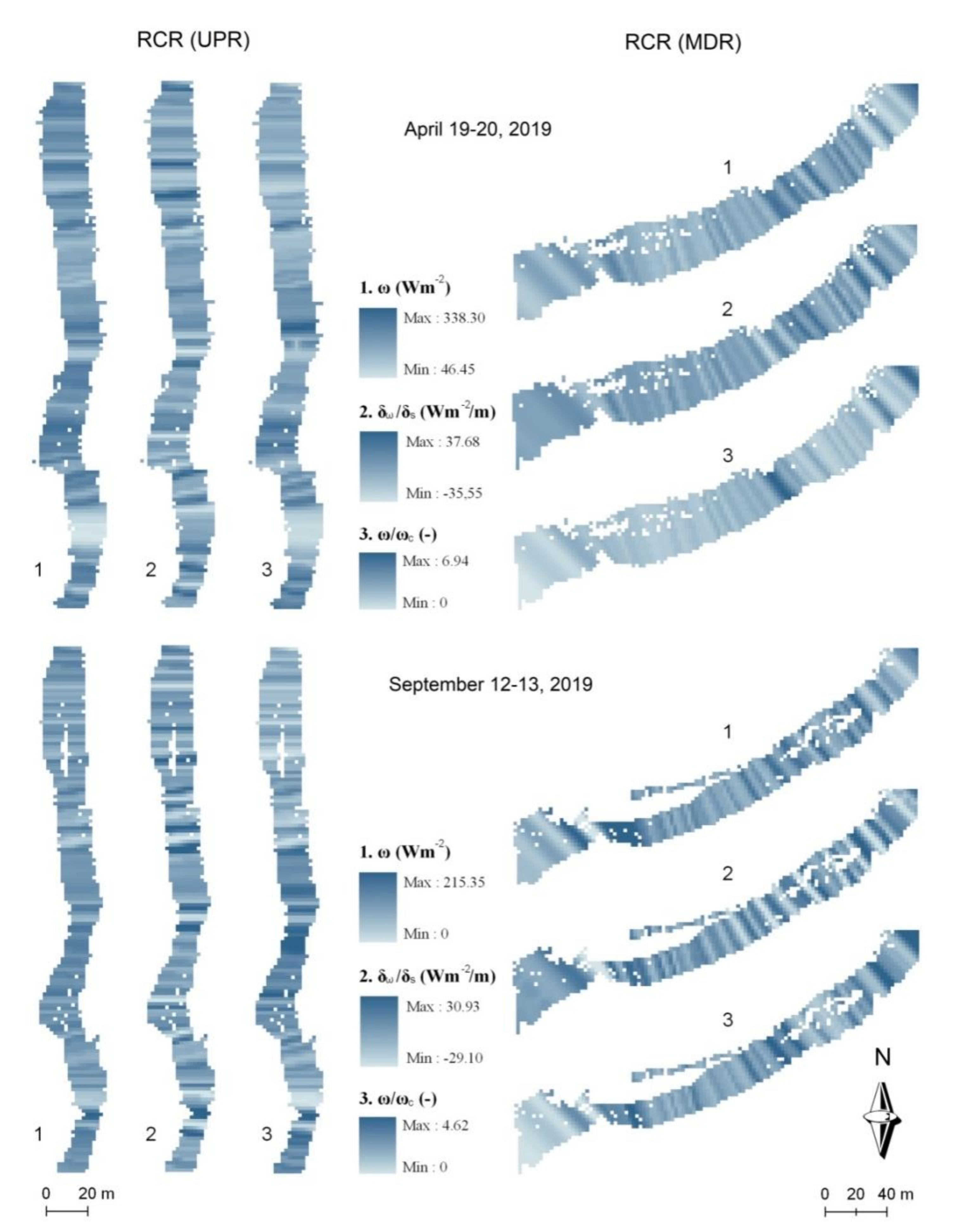
4.1. Stream Power Maps

The mean stream power (ω), energy gradient (∂ω/∂s), and mean stream power (ω)/resisting power (ωc) ratio (ω/ωc) were estimated discreetly along each of the RCR for the most significant flood events: 19–20 April 2019 and 12–13 September 2019. Figure 6 shows the grids of these variables for the UPR and MDR during these events. The resulting maps were then related to the spatial patterns of sediment budgets in order to explain better the processes that control the morphological channel adjustments.
In the study RCR, the ω during the peak flow of 19–20 April 2019 varied from 0.6 to 371.4 W m−2 and the stream power gradient from −40.8 to 51.2 Wm−3 (the upper limits of color displayed in Figure 6 for these variables encompass 95% of the data; that is, 338.3 Wm−2 and 37.7 Wm−3, respectively). Note, however, that more than 75% of the set of values of ∂ω/∂s in this event fell within the range 15 to −15 Wm−3 and that the extreme data reflect sharp local changes in ω. As in the case of the flow velocity and the shear stress, the highest values of ω were concentrated in entrenched channel cross-sections, along straight to slightly sinuous stretches, and locally over steep riffles characterized by high near-bed velocity gradients. This pattern is linked to incision processes in several Mediterranean ephemeral streams [35,55,56]. However, we observed a significantly different behavior in the gravel beds studied here, where important transitory erosion was often accompanied by extraordinary bedload mobility and high deposition rates, which tended to cause channel aggradation.
The distribution of the ω/ωc ratios was also skewed for both RCR and the flood events, with maximum values very distant from the mean and median. In the events of April and September, maximum ratios around 10 and 7 were reached, respectively, in the two reference stretches, with much lower and different medians depending on the section. Specifically, during the peak flood of 19–20 April 2019, the ω/ωc medians ranged from 2.7 in RCR (UPR) to 1.2 in RCR (MDR).

4.2. Spatial Sediment Budgets and Morphological Changes Along RCR and PBSA

4.2.1. Sediment Budgets in RCR Determined from SfMData

Gravel-bed erosion and aggradation are recurrent geomorphological processes that discretely affect the global evolution of ephemeral gravel-bed channels over time. Changes at the event scale are usually very disparate; in some cases, scour and downcutting phenomena predominate, and in others deposition. The present study contributes to a better understanding of the current behavior of this type of channel and the subsequent trend of its minor adjustments, but it contributes little in relation to possible long-term morphodynamic changes. A good indicator of these adjustments is the sediment budget in the reaches with the highest bedload. In particular, in the RCR analyzed here, the bedload experienced important spatial variations at the event scale, significantly affecting the sediment sources (areas of erosion) and sinks (areas of deposition) in the short period of analysis. In the September 2018–September 2019 stage, lateral erosion from steep alluvial banks, active low bars, partially destroyed coarse bar heads, and finer-grained bar tails provided a large bedload in the downstream direction. As a result, the greatest deposition thicknesses were recorded in the flanks of the longitudinal and medial alluvial bars, in both RCR (see Figure 7, drawn up on the basis of SfM-MVS data).
Previous field observations suggest that during low-water stages, as in the event of November 2018, when the top of the bar emerged, vertical accretion of these bars ceases and new secondary channels form, causing small island bars to migrate. The flash flood of 19–20 April 2019 resumed the aggradation process, with very widespread increases in bed height. The SfM statistical data in Table 1 show significant cumulative changes in ground surface elevation after the flow events of 19 November 2018 and 19–20 April 2019. An average net thickness difference of around 22 and 21 cm was found in the upper and middle reaches, respectively. The sedimentary balance was positive in both RCR, verifying a clear dominance of deposition over erosion. The proximity of both reaches to abundant sources of coarse sediment, mainly due to locally strong connectivity between the channel bed and active alluvial banks, together with a similar bed slope, promoting a notable mobility of the bedload, explains the scarce variation between the RCR in the average sediment budget. The high average deposition rate observed in the middle reach (unit TVSL = 0.218 m3 m−2) was not accompanied by equally significant unit volumes of erosion upstream (unit TVSR = 0.128 m3 m−2). This suggests that the sources of sediments include not only the upper RCR but also other more entrenched sections close to the headwater area and intermediate sections between the two RCR, where bank breaking and gravel bar removal are especially active processes. In addition, the minor unit net erosion recorded here during this event decreased even more downstream, reaching 0.086 m3 m−2 in the middle reach (Table 1), so the bed cutting could not progress in a downstream direction.
Heterogeneities due to differences in grain sizes and bedforms may create substantial velocity and shear stress variations across the channel or downstream during a single discharge [57]. This can explain the patchwork of ω values in both reaches (Figure 7) and, thus, the spatial changes in sediment budgets displayed in Table 1. The upper RCR registered the highest average unit volume of surface raising and lowering (0.13 and 0.23 m3 m−2, respectively), in line with the highest mean values of ω (72.4 Wm−2), but also the highest SD in the net thickness differences and in the ∂ω/∂s gradients (16.4 Wm−3).

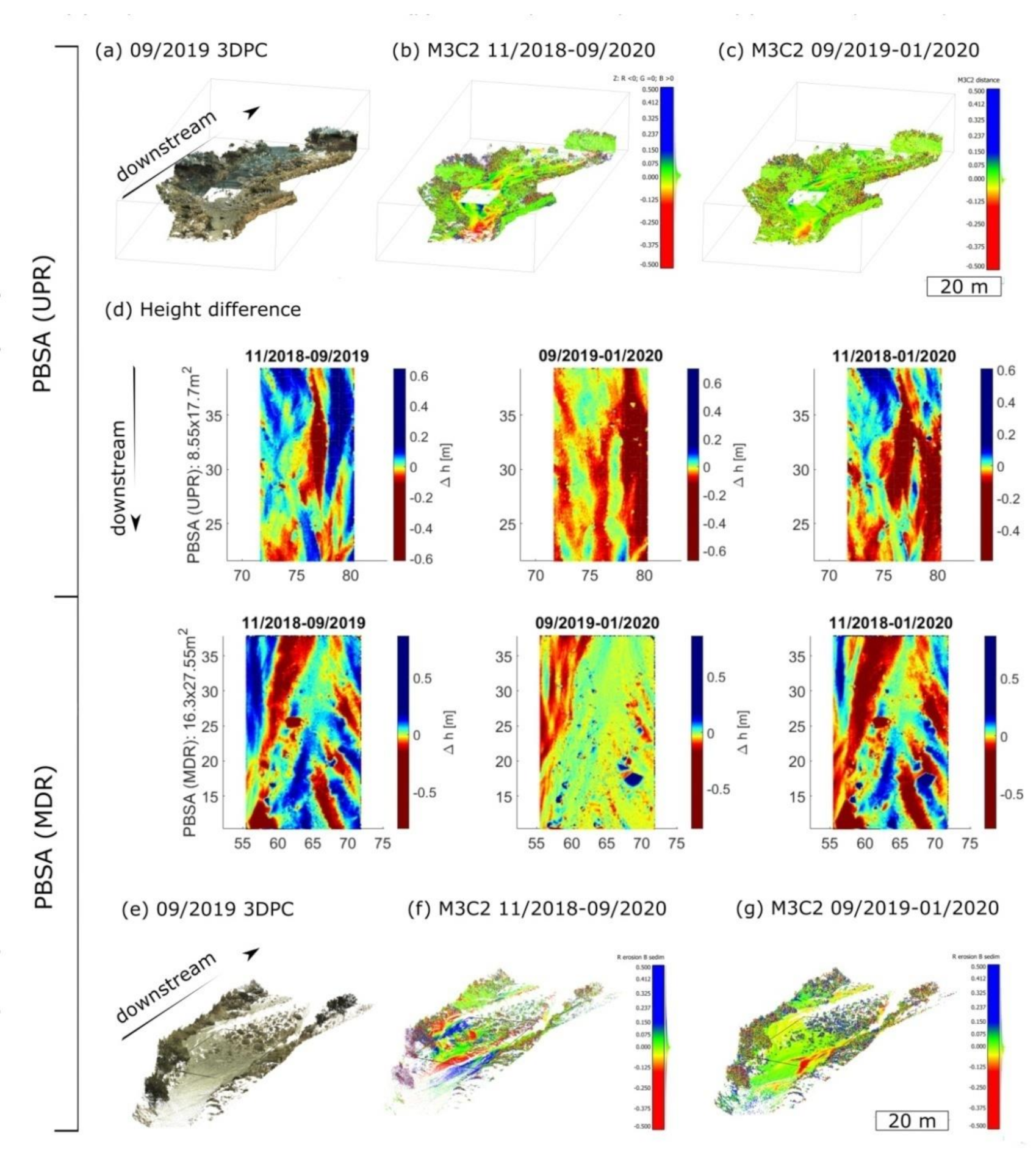
4.2.2. Sediment Budget and Stream Power in PBSA Estimated from TLS Data

The results in Table 1 (SfM-based results) differ from those obtained using TLS for the same reference channel reach during the period of December 2018 to September 2019, for two reasons. Firstly, there were differences caused by the fact that the UAV-SfM surveys included an event (the peak flow of November 18, 2018) that was not monitored with TLS. Secondly, it is widely accepted that the evaluation of sediment budgets is sensitive to differences in DTM quality and in the process used to suppress vegetation cover, since they inherently incorporate errors into the generated terrain models [54]. Although this type of error was considered small in the two reference reaches, given the high resolution of the DTMs used, this factor cannot be completely discounted in the more vegetated areas.
In addition, the high-density 3-D point clouds generated from TLS were applied to pilot bed areas (PBSAs) in order to detect detailed changes in bedload budgets. In Figure 8 and Figure 9 and Table 2, the results obtained during three periods are shown: November 2018–September 2019, September 2019–January 2020, and November 2018–January 2020. The first of these periods offers information on the morphological sediment budgets attributable to the flash flood of 19–20 April 2019; the second includes the peak flows of 12–13 September 2019 and 2 December 2019; and the third covers all three events. In the areas detailed, a positive balance was detected after the first event, with an average unit volume of 21.55 dm3 m−2 in PBAS (UPR) and 10.03 dm3 m−2 in PBAS (MDR), whereas there was a negative average balance during the second period, when erosion removed 54.12 and 26.25 dm3 m−2, respectively, in these two areas.
The analysis of budgets expressed in unit volume for 10-cm elevation intervals show that the largest volumetric variations implied morphological adjustments, ranging between −0.2 and +0.2 m in bed elevation (Table 2). Within these intervals, the greatest unit volume of deposition (41.3 dm3 m−2) corresponded to PBSA (MDR) after the April 2019 event, and the greatest erosion volume (48.9 dm3 m−2) to PBSA (UPR) after the two minor events of the period September 2019 to January 2020. These data are consistent with those displayed for both cases in the normalized histograms of elevation differences (Figure 9), where the interval from 0 to +0.2 m had a cumulative frequency greater than 60% and that from 0 to −0.2 m exceeded 70%.
Likewise, the variations and signs of the mean energy gradient faithfully reflected the different patterns observed in the bedload budgets of each PBSA. Assuming that ∂ω/∂s represents the clearest expression of sediment change in the nearest cell downstream, we can hypothesize that this hydraulic variable had a strong influence on the net erosion or deposition, and on the total mean bedload volume per unit area. However, while the net deposition pattern expected with a higher positive ∂ω/∂s did occur, the same did not happen with the net erosion pattern, since the most negative ∂ω/∂s registered in PBSA (UPR), during the flood peak on 19 April 2019, finally translated into a unit net volume of downcutting lower than the one accumulated by the minor events of September 2019 and January 2020. The larger flow event in April generated significantly higher mean ∂ω/∂s valuesthan the minor peak flow in September, with a negative sign in PBSA (UPR) and a positive one in PBSA (MDR), which resulted in a decrease from −3.8 to −0.4 Wm−3 for the first case and from 1.9 to 1.6 Wm−3 for the second (Table 3). This suggests that in the major event, a much larger bed load was mobilized and replaced than in the minor event, and that during the latter the energy expenditure was used for scouring and there was not enough surplus (ω/ωc = 1.6vs. 2.6 in the April flood) to drag and deposit the material transported from upstream.
Such results corroborate the hypothesis that in this ephemetal gravel-bed stream, the events of greater magnitude (Qp ≥30 m3 s−1) produce vertical sedimentary accretion on the bed [41], exceeding even the critical stress of the coarsest particles (gravel and pebbles) in PBSA (UPR) (mean ω/ωc >2) and thus moving a large bedload downstream. In contrast, more moderate peak flow rates (Qp ≤10 m3 s−1) were only able to exert a surface washing action, selective transport, and local scouring. In both cases, all the events analyzed tended to reinforce and arm the bed, as seen in situ, making it more resistant to erosion in future floods.

4.2.3. Morphological Bed Adjustments Observed in RCR from TLS Data

The detailed topographic survey performed for each channel reach prior to and following a bedload-transporting flow event made it possible to detect precise changes in channel morphology in relation to event-scale bedload fluxes. Such an approach was highly recommended by Kasprak et al. [53], when an HRDTM is available, and by Singer and Michaelides [58] for the case of ephemeral channels, where topography appears to remain unchanged.
In Figure 10, the morphological changes observed along the channel center line of both reference reaches using TLS datasets. From this, different patterns of spatial variability were inferred, depending on the reference site, the magnitude of the flood, and the textural and topographic characteristics immediately prior to the occurrence of each event.
In the upper RCR, the major morphological bed changes corresponded to two types of channel narrowing: at the exit of a meander and that due to structural control in less sinuous reaches. In the first case, the forms of excavation and vertical accretion reflected a marked bed alteration just 15 m in length, the incision prevailing in the largest event and the deposition in the least torrential (Figure 10c in UPR). In the second case, downstream narrowing, the major event caused significant variations in the topography of the bed, creating new active bars that later, in the event of September 2019, were partially or totally destroyed. These morphological adjustments must have been caused by high stream power values concentrated in short distances, as already suggested by Conesa-García et al. [59] for entrenched channel cross-sections, along stretches with sudden changes in bed roughness. This pattern has been found to be linked to channel degradation in semi-arid ephemeral streams (e.g., [35,56]).
However, we observed significantly different behavior in the gravel beds studied here, where important transitory erosion was often followed by considerable replenishment of coarse-grained sediments, finally producing bed aggradation. The rest of the stretch showed slight changes in the inter-bends or runs transition zones and significant homogeneous variation in the final part, where progressive erosion downstream caused by the flash flood of April 2019 was partially offset by aggradation processes during the following minor event.
The middle RCR presents two spatial patterns of geomorphic change: one of them around an extensive central bar (65 m long), characterized by important variations of different sign, depending on whether it is the anterior sector, the bar itself, or the posterior area in a downstream direction. At the back of the bar head, an incision of 0 to −0.5 m was observed, while the head and platform of the bar experienced vertical accretion in both events, and the tail suffered a lowering in height of up to −0.3 m. The minor event in September introduced hardly any variations in this reach except in the final part of the platform, which was lowered by around −0.4 m (Figure 10c in MDR). The second pattern, represented in the rest of the reference channel reaches, arises from a certain bed stability, only interrupted by slight alternative adjustments of incision and vertical accretion, resulting in net elevation differences between +0.2 and −0.2 m.

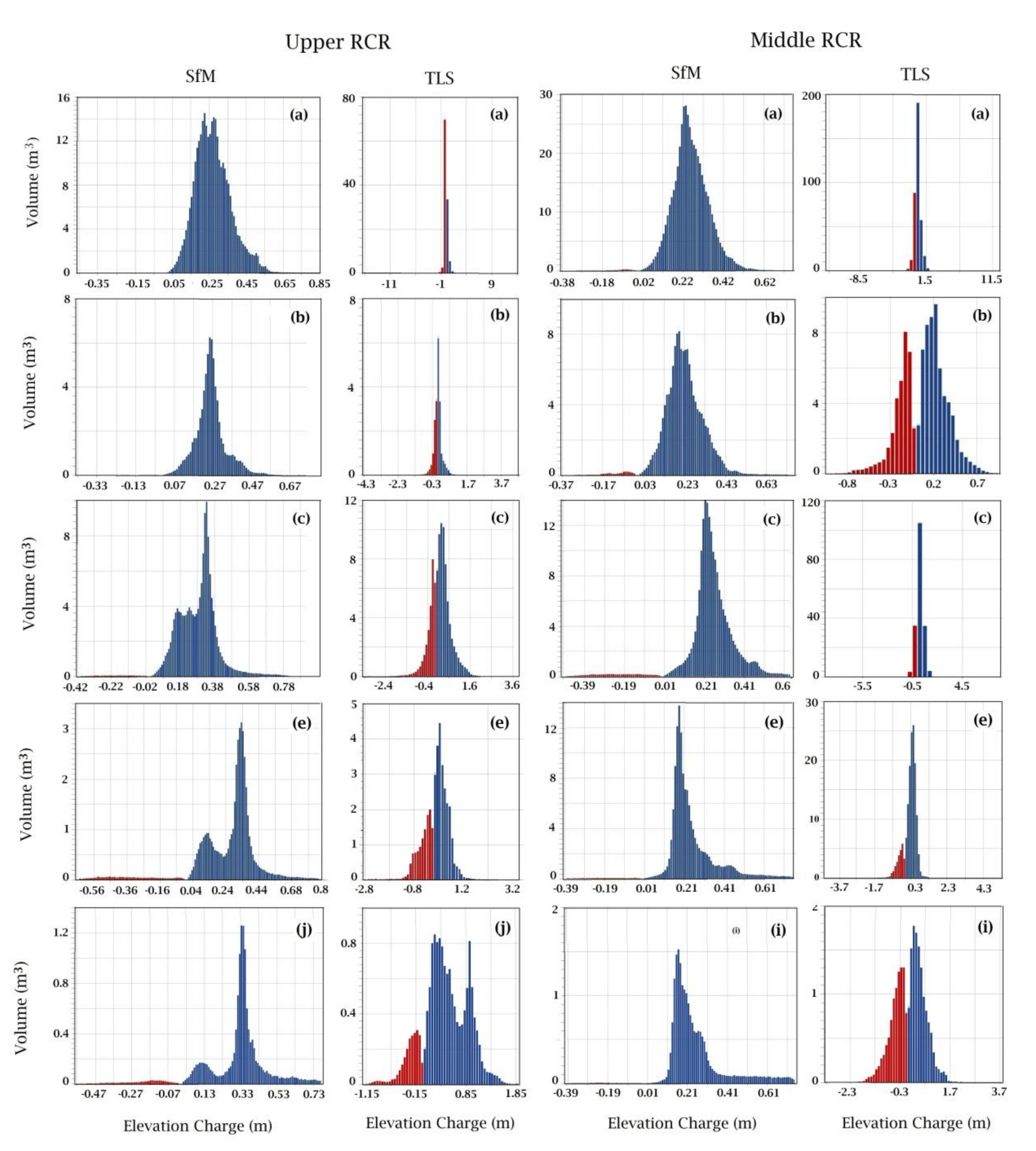
4.3. Sediment Budgets for Different RGUs in Relation to Stream Power Data and Field Surveys

In Table 4, standard variables commonly used in sediment budgeting (sediment area and volume) for each representative geomorphic unit (RGU) and RCR are shown, derived from SfM and TLS data, concerning the peak flows produced during their respective field surveys. As mentioned above, the SfM monitoring periods included one more event than those of the TLS; therefore, despite offering fairly similar surface area data for each RGU, they provided different volume data and errors.
Although the time interval considered (September 2018 to September 2019) is relatively short, and only covers one or two events, depending on the type of survey performed, the fact that almost all RGUs registered a positive total average balance in favor of deposition is striking (Table 4 and Figure 11). Only the inter-bar active bed in the upper RCR scored a slightly negative budget, according to the TLS data, after the flash flood of 19–20 April 2019. This result, added to the fact that the difference in average total thickness or the average unit volume difference for each RGU was always lower with TLS than with SfM, undoubtedly shows that the November 2018 peak flow, although lower than that of April 2019, also contributed to the deposition.
In summary, it can be considered that almost all the bed forms experienced over-sedimentation and, therefore, vertical accretion. The maximum accumulation produced after both events (0.18 to 0.23 m3/m2) took place on the active bed zones and on the scarcely vegetated gravel bars, which behaved as somewhat unstable forms (Table 4 and Figure 11). Even the main active bed in run stretches within the middle reach rose. The positive sediment budget in lateral tail and high bars could be misleading (average total thickness difference around 0.20 m), but, nevertheless, corresponds to local collapses of material caused by basal undermining in high detrital banks (Figure 12(1,2)) and lateral accretion by the adjoining of finer sediments (sand and gravel) in alternate and central bars (Figure 12(4)). However, this contribution was not sufficient to explain the large imbalance between the average volume of sediment returned to the channel through bank collapse (equivalent to 11% of the total flux) and the net volume of sand and gravel deposited on the bars (66% of the total budget).
Consequently, most of the bedload mobilized and deposited in both stream stretches could come from upper sediment sources, associated with intense downcutting processes in deep gullies that dissect the apical zone of thick alluvial fans. López-Bermúdez et al. [60], Harvey [61], and Aguilar et al. [62] found similar results when studying steep alluvial fans dissected by gullies in semi-arid and arid environments. Simultaneously, low-order gravel bed tributaries at the headwaters currently develop high geomorphic activity, leading to considerable variations in downstream sediment yield, which is consistent with the pattern described by Lisle et al. [63] and Yuill et al. [64] for this type of ephemeral gravel-bed channel.
By comparing the sediment budgets obtained using TLS after the flash flood of April 2019 with the stream power indicators referring to this event (see Figure 6), we observed that the ω/ωc ratio exerted a greater influence than ∂ω/∂s on the incision and vertical accretion processes, depending on the predominant type of RGU in each set of cells. Specifically, in sites with dominant changing RGU, such as active channel inter-bars or runs (a), low, active non-vegetated bars (b), and low, scarcely vegetated bars (c), strong relationships were found between the average total thickness difference and the ω/ωc ratio (r2 ≈ 0.89 in both channel reaches). The relationship of surface height change with ∂ω/∂s was also statistically significant but not as strong as that with the average relative excess energy (r2 = 0.83 and 0.66 in UPR and MDR respectively, p-value < 0.05 for the 95%confidence interval). In any case, a different behavior could be intuited in the most unstable bars of each of the RCR in relation to the ratios ∂ω/∂s and ω/ωc estimated for each channel stretch. In the upper RCR cell sets, where these RGUs predominated, average values of ∂ω/∂s and ω/ωc of −4.4 Wm−3 and 2.3, respectively, were found, which led to a slight lowering in the active bed (−0.024 m on overage) and a general increase in height of only 5 cm in longitudinal non-vegetated bars (Figure 12(4)). In contrast, smaller values of ∂ω/∂s and ω/ωc (−1.6 Wm−3 and 1.5, respectively) at the front and head of a mid-channel bar (central island), crossing the middle RCR, caused a thicker deposit (average bed rise of 11 to 15 cm) and greater morphological adjustments (Figure 12(5)).
Field observations immediately after this event showed that such sediment budgets were accompanied by a relocation of the bed material and changes in bed texture (Figure 12). Along all the upper RCR, riffles proved to be the most stable bedforms and preserved the coarsest particles. Additionally, a large amount of gravel was deposited on runs or pool exit-point bars in bed stretches, in agreement with the results obtained by Thompson et al. [65] and Wohl [57] in steep bed-gravel streams.
In the ascending part of the hydrograph, the steepened water-surface gradients over alternate bars and runs in the upper RCR must have promoted bed dissection and removal of finer particles, which were then stored in pools downstream. This geomorphic process was described by Lisle and Hilton [66] when studying the fine bed material in pools of natural gravel-bed channels.
Downstream, in the middle RCR, new deposits at the head of the mid-bar referred to earlier contributed to raising its surface, mainly with sand and fine gravel (Figure 12(5)). The somital platform of the central bar was not totally submerged, and acted as a roughness element that must have locally increased the vertical velocity of the flow on the flanks, in turn driving the lateral vortex cells, with the consequent start or reactivation of entrainment of the less coarse particles. As the flow cells enlarged and moved locally, incision occurred in secondary active channels around the bar, increasing the bedload pulses downstream.
A similar contrast is provided by the comparison of the differences in absolute net volumes with the corresponding variations in elevation (negative or positive) detected with SfM and TLS. The total net deposition volumes were considerably higher than the erosion in all RGUs and in both RCR, according to the SfM data. Among these bedforms, within the upper RCR, the active bed registered the highest absolute volume increase (12 to 14 m3), associated with bed raising of 0.2 to 0.3 m (Figure 13). Active bars and unstable scarcely vegetated low bars also experienced a significant increase in volume, but with different ranges of heights. The largest net deposition volumes (from 4 to 8 m3) meant increases in height from 0.15 to 0.30 m in the first case (leptokurtic distribution), and from 0.1 to 0.4 m in the second (dominant mesokurtic distribution). The high sparsely vegetated bars and vegetated tail only exhibited occasional variations that had little impact on the overall channel adjustments. The middle RCR showed a somewhat different pattern, characterized by Gaussian distributions and a single mode in most RGUs. Here, the active bed once again scored by far the highest volume charge, with maximums of 30 to 37 m3 accompanied by the same bed rises (0.20 to 0.35 m) as in the upper RCR. The rest of the bedforms received, with respect to the upstream reference reach, a greater sedimentary contribution that did not translate into substantial morphological changes since the accretion height hardly varied. The reason for this could be the greater wetted channel width and the presence of transverse and central bars in the middle RCR, compared to the relative channel narrowness and development of longitudinal bars in the upper reach.
The TLS results for the April event provided quite different patterns, with single-mode leptokurtic distributions in the most unstable bed forms: in a, b, and c of the upper RCR and in a and c of the middle RCR. The only exception was in the behavior of the active bars without vegetation, whose distribution showed two pointed curves in the central part, representing modes of erosion (average depth of lowering of −0.1 to −0.2 m) and deposition (average rise height of 0.20 to 0.35 m), respectively. This was probably due to unequal morphological adjustments, after transitory erosion occurred in both cases. Field observations verified lower rates of transitory erosion (only 5 cm for this event) in this morphosedimentary unit than in the active bed itself, where depths of 20 to 25 cm were reached (Figure 12(7)). In the rest of the RGUs, the net volumes of deposition exceeded those of erosion.
On a local scale, it is worth noting the bimodal distribution observed in the scarcely vegetated banks or tail, especially in the middle RCR, where the maximum volume of erosion supposed an average lowering of the bed surface of around 5 cm and that of deposition an average raising of 7 cm.
Consequently, all the patterns of spatial variability in the sediment budgets, described with SfM and TLS data, showed a clear tendency to increase bedload and granular bed armoring. The supplies of gravel in both RCR exceeded the volume of scour, causing an increasing alluvium that tends to make it more and more difficult to lower the bed surface by downcutting, increases the hydraulic resistance of the bed materials, and redirects the energy expenditure towards the banks. The result is a gradual widening of the channel and an increase in the width-to-depth ratio, particularly significant in sites of the middle and lower reaches, not subject to geological constrictions.

5. Conclusions

An excess or deficit of sediment in a sediment budget implies different responses of the channel morphology and bed forms. In the case of ephemeral gravel-bed streams, where the morphological adjustments are the product of complex flow dynamics at the event scale, the approach proposed here, based on the integrated use of UAV-SfM and TLS, has allowed this budget assessment to be satisfactorily addressed. Additionally, such an approach means economic savings and optimization of monitoring resources, through the synchronized application of both techniques, and the use of one or the other, depending on the magnitude of the event and the type of geomorphic change (overall channel adjustments or changes in bedforms). The SfM-MVS proved to be an appropriate technique for estimating sediment budgets in longer stream stretches, such as RCR over 100 m in length, while TLS provided excellent results for the determination of changes in bedload budgets at more detailed spatial scales (PBSA and RGU). Different complex morphodynamic processes, including total scouring-and-bedload transport and transitory erosion, which must have taken place simultaneously during each flood, could not be directly quantified. Nevertheless, the sediment budgets expressed in terms of net bed elevations and volumes were calculated with high accuracy for the wetted channel perimeter and the RGU during the monitored peak flows. This information was very useful, especially when coupled with in situ observations made after each event and the stream power parameters, obtained from the calibrated 1-D hydrodynamic model. The results from the study sites provided detailed information on the bed loading budgets, location of sediment sources and sinks, and changes in bedforms but also contributed to a better knowledge of the current morphodynamics of ephemeral gravel-bed channels in semi-arid Mediterranean coastal areas. With the support of field research, several hypotheses were verified, the most significant of which relates the magnitude of the events with the geomorphic process and morphological adjustments. Specifically, we found that flows exceeding bankfull discharge tend to produce vertical sedimentary accretion (0.20 to 0.35 m for a peak flow of 31 m3 s−1), after having mobilized a large amount of bedload upstream. Great variations in the stream power gradient and high average excess energy (−15< ∂ω/∂s <15 Wm−3; mean ω/ωc ratios>2 for the same event) occurred during this process. By contrast, more moderate peak discharges (≤10 m3 s−1) were only capable of exerting surface washing, selective transport, and local scouring, mainly affecting active low bars. The lowest net thickness of deposition detected by SfM and TLS in the upper stretch (less than 0.06 m) often masked an extraordinary mobility of the gravel deposits, crossing riffles and inter-bar runs, which could only be proved by measuring transitory erosion in the field (0.20 to 0.25 m at the upper RCR). Regardless of the magnitude of the monitored events, bed armoring was identified in situ, which tends to make the bed more resistant to erosion in future floods. If an increase in the frequency of flash floods due to climate change is confirmed in southeastern Spain, it is foreseeable that in the short and medium term, the trend of bed aggradation will continue in these ephemeral gravel streams, fed by the increasing inputs of coarse particles from the slopes, thus promoting lateral erosion and widening the channel, as has already occurred in more arid environments.

Author Contributions

Conceptualization, C.C.-G.; methodology, C.C.-G., A.R., R.T., R.G.-L. and P.P.-C.; data acquisition, C.C.-G., A.R., R.T., J.L.P., M.C.G., F.M.-C. and C.P.-M.; formal analysis, C.C.-G., A.R., R.T., C.P.-M., P.P.-C. and R.G.-L.; writing—original draft preparation, C.C.-G.; writing—review and editing, C.C.-G., A.R., R.T., J.L.P., M.C.G., F.M.-C. and R.G.-L.; supervision, C.C.-G.; project administration, C.C.-G.; funding acquisition, C.C.-G. All authors have read and agreed to the published version of the manuscript.

Funding

This research was funded by ERDF/Spanish Ministry of Science, Innovation and Universities - State Research Agency/Project CGL2017-84625-C2-1-R (CCAMICEM); State Program for Research, Development and Innovation Focused on the Challenges of Society, the Spanish Ministry of Economy and Competitiveness (MINECO) and EU FEDER under Project TEC2017-85244-C2-1-P and by the University of Alicante (vigrob-157 and GRE18-05).

Acknowledgments

We would like to thank the Segura River Hydrographic Confederation Center (SHC), Government of Spain, for its collaboration.

Conflicts of Interest

The authors declare no conflict of interest.

Notation

D50median grain size (m)
D84particle size corresponding to the 84% of the sample weight (m)
∂ω/∂s mean stream power gradient [Wm−3]
γspecific weight of water (Nm−3),
icell at i cross-section
Ωcross-sectional stream power [W m−1]
ωmean stream power [Wm−2]
ωccritical mean stream power [W m−2]
qppeak unit flow (m3 s−1)
r2determination coefficient
Swwater surface slope [m m−1]
tbbase time (h)
tb* base time of the unit hydrograph (h)
thhydrograph duration (h)
tptime of peak (h)
tp* time of peak of the unit hydrograph (h)
wwater-surface width (m)
ADLAverage depth of lowering
ADRAverage depth of raising
ANTDAverage net thickness difference (m) for the area of interest
ATTD Average total thickness difference (m) for area of interest
3DPC 3D point cloud
FSField survey
GCPs Ground Control Points
GNSSGlobal Navigation Satellite System
HRDTMHigh-resolution Digital Terrain Models
MDRMiddle reach
MVSMulti-View Stereo
OVROverall channel reach
PBSAPilot bed survey area
PI Percent imbalance (departure from equilibrium)
RCRReference channel reach
RGURepresentative geomorphic unit
RPASRemotely Piloted Air Systems
SfMStructure from Motion
TAITotal area of interest (m2)
TASLTotal area of surface lowering (m2)
TASRTotal area of surface raising (m2)
TLSTerrestrial Laser Scanner
TNVD Total net volume difference (m3)
TVDA Total volume difference average (m3)
UAVUnmanned aerial vehicles
UPRUpper reach
UVSLAverage unit volume of surface lowering (m3 m−2)
UVSRAverage unit volume of surface raising (m3 m−2)
SD *Standard deviation of the net thickness differences (m)

References

  1. Segura-Beltrán, F.; Sanchis-Ibor, C. Assessment of channel changes in a Mediterranean ephemeral stream since the early twentieth century. The Rambla de Cervera, eastern Spain. Geomorphology 2013, 201, 199–214. [Google Scholar] [CrossRef]
  2. Conesa-Garcia, C. Torrential flow frequency and morphological adjustments of ephemeral channels in southeast Spain. In River Geomorphology; Hickin, E.J., Ed.; John Wiley & Sons: Chichester, UK, 1995; pp. 169–192. [Google Scholar]
  3. Sutfin, N.A.; Shaw, J.; Wohl, E.E.; Cooper, D. A geomorphic classification of ephemeral channels in a mountainous, arid region, southwestern Arizona, USA. Geomorphology 2014, 221, 164–175. [Google Scholar] [CrossRef]
  4. Norman, L.M.; Sankey, J.B.; Dean, D.; Caster, J.; Delong, S.; Delong, W.; Pelletier, J.D. Quantifying geomorphic change at ephemeral stream restoration sites using a coupled-model approach. Geomorphology 2017, 283, 1–16. [Google Scholar] [CrossRef]
  5. Graf, W.L. Fluvial Processes in Dryland Rivers; Springer: New York, NY, USA, 1988. [Google Scholar]
  6. Bull, L.J.; Kirkby, M.J. Dryland rivers characteristics and concepts. In Dryland Rivers: Hydrology and Geomorphology of Semi-arid Channels; Bull, L.J., Kirkby, M.J., Eds.; John Wiley & Sons: Chichester, UK, 2002; pp. 3–15. [Google Scholar]
  7. Török, G.; Baranya, S.; Rüther, N. 3D CFD Modeling of Local Scouring, Bed Armoring and Sediment Deposition. Water 2017, 9, 56. [Google Scholar] [CrossRef] [Green Version]
  8. Goodrich, D.C.; Lane, L.J.; Shillito, R.M.; Miller, S.N.; Syed, K.H.; Woolhiser, D.A. Linearity of basin response as a function of scale in a semiarid watershed. Water Resour. Res. 1997, 33, 2951–2965. [Google Scholar] [CrossRef]
  9. Shaw, J.R.; Cooper, D.J. Linkages among watersheds, stream reaches, and riparian vegetation in dryland ephemeral stream networks. J. Hydrol. 2008, 350, 68–82. [Google Scholar] [CrossRef]
  10. Merritt, D.M.; Wohl, E.E. Downstream hydraulic geometry and channel adjustment during a flood along an ephemeral, arid-region drainage. Geomorphology 2003, 52, 165–180. [Google Scholar] [CrossRef]
  11. Camporeale, C.; Perona, P.; Ridolfi, L. Hydrological and geomorphological significance of riparian vegetation in drylands. In Dryland Ecohydrology; D’Odorico, P., Porporato, A., Eds.; Springer: Dordrecht, The Netherlands, 2006; pp. 161–179. [Google Scholar]
  12. Reid, I.; Frostick, L.E. Channel form, flows and sediments of endogenous ephemeral rivers in deserts. In Arid Zone Geomorphology: Process, Form and Change in Drylands; Thomas, D.S.G., Ed.; John Wiley & Sons: Chichester, UK, 2011; pp. 301–332. [Google Scholar]
  13. Martín-Vide, J.P. Ingeniería Fluvial; UniversitatPolitècnica de Catalunya: Barcelona, Spain, 1997; ISBN 9788498801569. [Google Scholar]
  14. Chen, S.A.; Michaelides, K.; Grieve, S.W.D.; Singer, M.B. Aridity is expressed in river topography globally. Nature 2019, 573, 573–577. [Google Scholar] [CrossRef] [Green Version]
  15. Brasington, J.; Vericat, D.; Rychkov, I. Modeling river bed morphology, roughness, and surface sedimentology using high resolution terrestrial laser scanning. Water Resour. Res. 2012, 48. [Google Scholar] [CrossRef] [Green Version]
  16. Picco, L.; Mao, L.; Cavalli, M.; Buzzi, E.; Rainato, R.; Lenzi, M.A. Evaluating short-term morphological changes in a gravel-bed braided river using terrestrial laser scanner. Geomorphology 2013, 201, 323–334. [Google Scholar] [CrossRef]
  17. Calle, M.; Alho, P.; Benito, G. Monitoring ephemeral river changes during floods with SfM photogrammetry. J. Iber. Geol. 2018, 44, 355–373. [Google Scholar] [CrossRef]
  18. Flatley, A.; Rutherfurd, I. Using Structure from Motion (SfM) to capture high resolution geomorphic units within small ephemeral channels. In Proceedings of the 20th EGU General Assembly, Vienna, Austria, 7–12 April 2019. [Google Scholar]
  19. Galea, A.B.; Sadler, J.P.; Hannah, D.M.; Datry, T.; Dugdale, S.J. Mediterranean intermittent rivers and ephemeral streams: Challenges in monitoring complexity. Ecohydrology 2019, 12, e2149. [Google Scholar]
  20. Clapuyt, F.; Vanacker, V.; Van Oost, K. Reproducibility of UAV-based earth topography reconstructions based on Structure-from-Motion algorithms. Geomorphol. 2016, 260, 4–15. [Google Scholar] [CrossRef]
  21. Marteau, B.; Vericat, D.; Gibbins, C.; Batalla, R.J.; Green, D.R. Application of Structure-from-Motion photogrammetry to river restoration. Earth Surf. Process. Landforms 2016, 42, 503–515. [Google Scholar]
  22. Remondino, F.; Barazzetti, L.; Nex, F.; Scaioni, M.; Sarazzi, D. UAV photogrammetry for mapping and 3d modeling–current status and future perspectives. ISPRS Int. Arch. Photogramm. Remote Sens. Spat. Inf. Sci. 2011, 38, 25–31. [Google Scholar]
  23. Shintani, C.; Fonstad, M.A. Comparing remote-sensing techniques collecting bathymetric data from a gravel-bed river. Int. J. Remote Sens. 2017, 38, 2883–2902. [Google Scholar] [CrossRef]
  24. Legleiter, C.J.; Harrison, L.R. Remote Sensing of River Bathymetry: Evaluating a Range of Sensors, Platforms, and Algorithms on the Upper Sacramento River, California, USA. Water Resour. Res. 2019, 55, 2142–2169. [Google Scholar] [CrossRef]
  25. Tonina, D.; McKean, J.A.; Benjankar, R.M.; Wright, C.W.; Goode, J.R.; Chen, Q.; Reeder, W.J.; Carmichael, R.A.; Edmondson, M.R. Mapping river bathymetries: Evaluating topobathymetric LiDAR survey. Earth Surf. Process. Landf. 2019, 44, 507–520. [Google Scholar]
  26. Mosbrucker, A.R.; Major, J.J.; Spicer, K.R.; Pitlick, J. Camera system considerations for geomorphic applications of SfM photogrammetry. Earth Surf. Process. Landf. 2017, 42, 969–986. [Google Scholar]
  27. Salmela, J.; Kasvi, E.; Vaaja, M.T.; Kaartinen, H.; Kukko, A.; Jaakkola, A.; Alho, P. Morphological changes and riffle-pool dynamics related to flow in a meandering river channel based on a 5-year monitoring period using close-range remote sensing. Geomorphology 2020, 352, 106982. [Google Scholar] [CrossRef]
  28. Rowley, T.; Ursic, M.; Konsoer, K.; Langendon, E.; Mutschler, M.; Sampey, J.; Pocwiardowski, P. Comparison of terrestrial lidar, SfM, and MBES resolution and accuracy for geomorphic analyses in physical systems that experience subaerial and subaqueous conditions. Geomorphology 2020, 355, 107056. [Google Scholar] [CrossRef]
  29. Cook, K.L. An evaluation of the effectiveness of low-cost UAVs and structure from motion for geomorphic change detection. Geomorphology 2017, 278, 195–208. [Google Scholar] [CrossRef]
  30. Vázquez-Tarrío, D.; Borgniet, L.; Liébault, F.; Recking, A. Using UAS optical imagery and SfM photogrammetry to characterize the surface grain size of gravel bars in a braided river (Vénéon River, French Alps). Geomorphology 2017, 285, 94–105. [Google Scholar] [CrossRef]
  31. Conesa-García, C.; Pérez-Cutillas, P.; García-Lorenzo, R.; Gómez-Gutiérrez, Á.; Eekhout, J.; Ibisate, A.; Ollero, A.; Horacio, J. Mapping spatial patterns of dimensionless ratios along an ephemeral channel using SfM photogrammetry. Geophys. Res. Abstr. 2019, 21, EGU2019. Available online: https://meetingorganizer.copernicus.org/EGU2019/EGU2019-7613-1.pdf (accessed on 23 May 2020).
  32. French, J.R. Airborne LiDAR in support of geomorphological and hydraulic modelling. Earth Surf. Process. Landf. 2003, 28, 321–335. [Google Scholar] [CrossRef]
  33. Heritage, G.L.; Hetherington, D. Towards a protocol for laser scanning in fluvial geomorphology. Earth Surf. Process. Landf. 2007, 32, 66–74. [Google Scholar] [CrossRef]
  34. Notebaert, B.; Verstraeten, G.; Govers, G.; Poesen, J. Qualitative and quantitative applications of LiDAR imagery in fluvial geomorphology. Earth Surf. Process. Landf. 2009, 34, 217–231. [Google Scholar] [CrossRef]
  35. Ortega, J.A.; Razola, L.; Garzón, G. Recent human impacts and change in dynamics and morphology of ephemeral rivers. Nat. Hazards Earth Syst. Sci. 2014, 14, 713–730. [Google Scholar] [CrossRef] [Green Version]
  36. Eisenbeiss, H.; Sauerbier, M. Investigation of UAV systems and flight modes for photogrammetric applications. Photogramm. Rec. 2011, 26, 400–421. [Google Scholar] [CrossRef]
  37. Puig-Mengual, C.A.; Martínez-Capel, F.; Woodget, A.S.; Muñoz-Mas, R. DEM generation in a Mediterranean river using Structure From Motion algorithm on HD video recorded from a UAV (Palancia River, Spain). In Proceedings of the HydroSenSoft, International Symposium and Exhibition on Hydro-Environment Sensors and Software, Madrid, Spain, 28 February–3 March 2017. [Google Scholar]
  38. Woodget, A.S.; Austrums, R. Subaerial Gravel Size Measurement Using Topographic Data Derived from a UAV-SfM Approach. Earth Surf. Process. Landf. 2017, 42, 1434–1443. [Google Scholar] [CrossRef]
  39. CloudCompare. Available online: http://cloudcompare.org/ (accessed on 25 February 2020).
  40. Brodu, N.; Lague, D. 3D terrestrial lidar data classification of complex natural scenes using a multi-scale dimensionality criterion: Applications in geomorphology. ISPRS J. Photogramm. Remote Sens. 2012, 68, 121–134. [Google Scholar] [CrossRef] [Green Version]
  41. Zapico, I.; Laronne, J.B.; Lucía, A.; Martín-Duque, J.F. Morpho-textural implications to bedload flux and texture in the sand-gravel ephemeral Poveda Gully. Geomorphology 2018, 322, 53–65. [Google Scholar] [CrossRef] [Green Version]
  42. Ali, K.F.; De Boer, D.H. Construction of sediment budgets in large-scale drainage basins: The case of the upper Indus River. In Proceedings of the Erosion Prediction in Ungauged Basins: Integrating Methods and Techniques, Montpellier, France, 8–9 July 2003. [Google Scholar]
  43. Scharffenberg, W.A.; Fleming, M.J. Hydrologic Modelling System HEC-HMS. User‘s Manual. Version 3.5.; US Army Corps of Engineers: Davis, CA, USA, 2010. [Google Scholar]
  44. Proyecto NATMUR-08 Catálogo de Geoservicios de Medio Natural, Vuelofotogramétrico Digital y levantamiento LIDAR de la Región de Murcia. Available online: http://www.murcianatural.carm.es/natmur08/ (accessed on 2 September 2018).
  45. Nanía, L.S. Manual Básico de HEC-HMS 3.0.0 y HEC-GeoHMS 1.1; Granada. 2007. Available online: http://www.ugr.es/~lnania/_private/ManualBasico_HEC-HMS300_HEC-GeoHMS11_Espanol.pdf (accessed on 10 October 2018).
  46. SCS (Soil Conservation Service). National Engineering Handbook; Section 4.; U.S. Department of Agriculture: Washington, DC, USA, 1972. Available online: https://directives.sc.egov.usda.gov/OpenNonWebContent.aspx?content=18393.wba (accessed on 5 November 2018).
  47. Nanía, L.S.; Gómez Valentín, M. IngenieríaHidrológica; Grupo Editorial Universitario: Granada, Spain, 2006; ISBN 84-8491-636-7. Available online: https://www.ugr.es/~lnania/ingenieria_hidrologica.htm (accessed on 2 September 2018).
  48. USACE (US Army Corps of Engineers). HEC-RAS, Rivers Analysis System. Hydraulic Reference Manual, Version 5.0; Hydrologic Engineering Center: Davis, CA, USA, 2016. [Google Scholar]
  49. Leopold, L.B.; Wolman, M.G.; Miller, J.P. Fluvial Processes in Geomorphology; Dover Publications: New York, NY, USA, 1964. [Google Scholar]
  50. Lea, D.M.; Legleiter, C.J. Mapping spatial patterns of stream power and channel change along a gravel-bed river in northern Yellowstone. Geomorphology 2016, 252, 66–79. [Google Scholar] [CrossRef]
  51. Parker, C.; Clifford, N.J.; Thorne, C.R. Understanding the influence of slope on the threshold of coarse grain motion: Revisiting critical stream power. Geomorphology 2011, 126, 51–65. [Google Scholar] [CrossRef]
  52. Wasson, R.J. Sediment budgets, dynamics, and variability: New approaches and techniques. In Proceedings of the The Structure, Function and Management Implications of Fluvial Sedimentary Systems; IAHS Publication: Alice Springs, Australia, 2002. [Google Scholar]
  53. Kasprak, A.; Wheaton, J.M.; Ashmore, P.E.; Hensleigh, J.W.; Peirce, S. The relationship between particle travel distance and channel morphology: Results from physical models of braided rivers. J. Geophys. Res. Earth Surf. 2015, 120, 55–74. [Google Scholar] [CrossRef]
  54. Brasington, J.; Langham, J.; Rumsby, B. Methodological sensitivity of morphometric estimates of coarse fluvial sediment transport. Geomorphology 2003, 53, 299–316. [Google Scholar] [CrossRef]
  55. Garzón, G.; Alonso, A. Comparison of the flood response of a braided and a meandering river, conditioned by anthropogenic and climatic changes. In Flood and Megaflood Processes and Deposits: Recent and Ancient Examples; Martini, I.P., Baker, V.R., Garzón, G., Eds.; Blackwell Publishing Ltd.: Oxford, UK, 2002; p. 320. [Google Scholar]
  56. Hooke, J.M. Human impacts on fluvial systems in the Mediterranean region. Geomorphology 2006, 79, 311–335. [Google Scholar] [CrossRef]
  57. Wohl, E. Mountain Rivers; American Geophysical Union: Washington, DC, USA, 2000. [Google Scholar]
  58. Singer, M.B.; Michaelides, K. How is topographic simplicity maintained in ephemeral dryland channels? Geology 2014, 42, 1091–1094. [Google Scholar] [CrossRef]
  59. Conesa-García, C.; Pérez-Cutillas, P.; García-Lorenzo, R.; Eekhout, J.; Gómez-Gutiérrez, Á; Millares-Valenzuela, A.; Martínez-Salvador, A. Dimensionless morphological ratios versus stream power variations at bankfull stage in an ephemeral channel. Geomorphology 2020, 361, 19. [Google Scholar]
  60. López-Bermúdez, F.; Boix-Fayos, C.; Solé-Benet, A.; Albaladejo, J.; Barberá, G.G.; Del Barrio, G.; Castillo, V.; Garcia, J.; Lázaro, R.; Martínez-Mena, M.D.; et al. Landscapes and desertification in south-east Spain overview and field sites. In Proceedings of the Sixth International Conference on Geomorphology, Zaragoza, Spain, 7–11 September 2005; p. 40. [Google Scholar]
  61. Harvey, A. Dryland Alluvial Fans. In Arid Zone Geomorphology: Process, Form and change in Drylands; John Wiley & Sons, Ltd.: Chichester, UK, 2011; pp. 333–371. [Google Scholar]
  62. Aguilar, G.; Cabré, A.; Fredes, V.; Villela, B. Erosion after an extreme storm event in an arid fluvial system of the southern Atacama Desert: An assessment of the magnitude, return time, and conditioning factors of erosion and debris flow generation. Nat. Hazards Earth Syst. Sci. 2020, 20, 1247–1265. [Google Scholar] [CrossRef]
  63. Lisle, T.E.; Nelson, J.M.; Pitlick, J.; Madej, M.A.; Barkett, B.L. Variability of bed mobility in natural, gravel-bed channels and adjustments to sediment load at local and reach scales. Water Resour. Res. 2000, 36, 3743–3755. [Google Scholar] [CrossRef]
  64. Yuill, B.; Nichols, M.; Yager, E. Coarse bed material patch evolution in low-order, ephemeral channels. Catena 2010, 81, 126–136. [Google Scholar] [CrossRef]
  65. Thompson, D.M.; Wohl, E.E.; Jarrett, R.D. A revised velocity-reversal and sediment-sorting model for a high-gradient, pool-riffle stream. Phys. Geogr. 1996, 17, 142–156. [Google Scholar] [CrossRef]
  66. Lisle, T.E.; Hilton, S. Fine bed material in pools of natural gravel bed channels. Water Resour. Res. 1999, 35, 1291–1304. [Google Scholar] [CrossRef]
Figure 1. Study area and location of the different channel stretches monitored by UAV-SfM and TLS during the period September 2018 to January 2020.
Remotesensing 12 03624 g001
Figure 2. Chronogram of the flow events and of the field surveys (FSs) performed using either UAV-SfM (Structure from Motion based on information collected with UAVs), Terrestrial Laser Scanning (TLS),or the combination of the two techniques (UAV—SfM + TLS). P = precipitation (mm); Qp—MDR = peak discharge (m3 s−1) at the Middle Reach; Qp—UPR = peak discharge (m3 s−1) at the Upper Reach.In parentheses, the maximum rainfall intensity (mm h−1).
Remotesensing 12 03624 g002
Figure 3. (a) View of the raw 3DPC; (b) 3DPC classified by means of the CANUPO plugin of CloudCompare, showing in blue the points classified as ground and in red those classified as vegetation; (c) 3DPC after removal of the points classified as vegetation; (d) the previous 3DPC rasterized using the rasterization tool of CloudCompare, computing the average height for each 5-cm cell and interpolating the empty cells with the nearest neighbors.
Remotesensing 12 03624 g003
Figure 4. Hydrographs and associated parameters for the flood events of 19–20 April 2019 and 12–13 September 2019, estimated in intermediate cross-sections of the UPR and MDR stretches. Q = discharge (m3 s−1); tp = time of peak (h); tb = base time (h); th = hydrograph duration (h); tp* and tb* = time of peak and base time of the unit hydrograph (h).
Remotesensing 12 03624 g004
Figure 5. RGU extracted within the boundaries defining each peak flow in the Upper and Middle RCR: a. Active channel, secondary minor channel inter-bars or run; b. Low, active non-vegetated bar; c. Low, scarcely vegetated bar; d. High, active non-vegetated bar; e. High, scarcely vegetated bar; f. High, vegetated bar; g. Non-vegetated talus or steep bank; h. Non-vegetated steep bank with falling rock blocks; i. Scarcely vegetated talus or steep bank.
Remotesensing 12 03624 g005
Figure 6. Values of ω, ∂ω/∂s, and ω/ωc obtained for each cell by spatial interpolation of HEC-RAS data related to equidistant (2.0–3.5 m) cross-sections in the RCR(UPR) and RCR(MDR). Peak floods of 19–20 April 2019 (upper graph) and 12–13 September, 2019 (lower graph). The maximum color limits encompass the 95% of the data sets.
Remotesensing 12 03624 g006
Figure 7. Surface elevation differences (m) found for the Upper (UPR) and Middle (MDR) RCR, using HRDTM derived from SfM-MVS, for the period September 2018 to September 2019, including the events of 18 November 2018 and 19–20 April 2019.
Remotesensing 12 03624 g007
Figure 8. (a) View of 3DPC captured in 2019; (b,c) M3C2 comparison of the 2018–2019 and 2019–2020 3DPCs, respectively; (d) height difference between 2018, 2019, and 2020 in the Upper and Middle PBSA; (e) view of 3DPC captured in 2019; (f,g) M3C2 comparison of the 2018–2019 and 2019–2020 3DPCs respectively.
Remotesensing 12 03624 g008
Figure 9. Normalized histograms of the elevation differences shown in Figure 8 for the Upper and Middle PBSA, comparing the 2018, 2019, and 2020 3DPCs.
Remotesensing 12 03624 g009
Figure 10. Thickness of the bed elevation differences caused by the flow peak of September 2019 in relation to those attributed to the flood of April 2019, using gross data with a 10-cm interval (a) and moving averages of band 9 (b) along the channel center line. The type (c) profiles represent the incision and aggradation sites for both peak flows with a band 9 smoothing. The profiles are based on TLS datasets.
Remotesensing 12 03624 g010
Figure 11. Average depth of lowering (ADL) and raising (ADR) and average total thickness difference (ATTD) obtained from SfM-MVS and TLS for the GRUs in the Upper and Middle RCR, after the peak flow of 19–20 April 2019. Letters refer to the RGU according to the legend in Figure 5.
Remotesensing 12 03624 g011
Figure 12. Local material collapses in composite detrital banks after basal undermining caused by the flash flood of April 2019 (1,2); entrainment and surface washing of non-cohesive basal bank deposits during the peak flow of September 2019 (3); after the larger event, greater morphological adjustments occurred: lateral accretion of central longitudinal bars in the Upper RCR (4), vertical accretion at the head of a central bar and slight incision on the thalweg bed in MDR (5), a strong net deposition between the upper and Middle RCR (see the levelogger plate that was deeply buried) (6), and high transitory erosion in the main active channel (see a clear example in the Upper RCR) (7).
Remotesensing 12 03624 g012
Figure 13. Differences in absolute net volumes versus variations in elevation (lowering and raising) of the bed surface detected with SfM and TLS for each GRU in the Upper and Middle RCR, after the peak flow of 19–20 April 2019. Letters refer to the RGU according to the legend in Figure 5.
Remotesensing 12 03624 g013
Table 1. Statistical descriptors relating to the morphological sediment budgets calculated for the overall (OVR) and reference channel reaches (RCRs) in the UPR and MDR for the period September 2018 to September 2019 (SfM data).
StatisticalTAITNVDANTDPITASLTASRUVSLUVSRSD*
Channel Reach Typem2m3% Errorm% Error% Valuem2m2m3 m−2% Errorm3 m−2% Errorm
UPROVR46579580.0450.2060.0450.470372842850.0830.1070.2310.0430.137
RCR27636140.0440.2220.0440.4866726950.1280.0690.2310.0430.118
MDROVR872020930.0400.2400.0400.48923484860.1030.0860.2490.0400.121
RCR488510130.0460.2070.0460.48616847170.0860.1020.2180.0460.106
TAI = Total Area of Interest (m2); TNVD =Total Net Volume Difference (m3); ANTD =Average Net Thickness Difference (m) for the Area of Interest; PI =Percent Imbalance (departure from equilibrium); TASL =Total Area of Surface Lowering (m2); TASR =Total Area of Surface Raising (m2); UVSL = Average Unit Volume of Surface Lowering (m3 m−2); UVSR = Average Unit Volume of Surface Raising (m3 m−2); SD * =Standard Deviation of the Net Thickness Differences (m); UPR = Upper reach; MDR = Middle reach; OVR = Overall channel reach; RCR = Reference channel reach.
Table 2. Changes in unit volume (dm3 m−2) and total mean volume per budget cell (dm3) obtained for elevation intervals of 10 cm and global height differences (Δe) in each pilot bed survey area (PBSA), based on TLS datasets covering the periods 2018–2019 1, 2019–2020 2, and 2018–2020 3.
Unit Volume (dm3 m−2)Total Mean Volume per Budget Cell (dm3)
PBSA (UPR)PBSA (MDR)PBSA (UPR)PBSA (MDR)
Δe
(m)
2018
20191
2019
20202
2018
20203
2018
20191
2019
20202
2018
20203
2018
20191
2019
20202
2018
20203
2018
20191
2019
20202
2018
20203
−0.5/−0.4−0.05−0.15−0.05−3.59−0.15−3.15−1.9−5.3−2.1−312.7−10.0−243.5
−0.4/−0.30.00−0.21−0.02−2.46−0.02−4.650.0−7.4−0.6−214.1−1.3−359.1
−0.3/−0.2−1.47−7.67-4.80−3.86−0.23−8.83−59.4−270.0−181.1−335.7−15.8−682.3
−0.2/−0.1−6.60−22.54−22.90−16.14−9.35−19.74−266.0−793.6−865.0−1405.4−631.2−1525.8
−0.1/0−11.32−26.36−19.95−11.35−23.91−14.32−456.4−928.4−753.6−987.7−1613.6−1106.5
ΔV<0−19.44−56.93−47.72−37.40−33.66−50.69−783.7−2004.7−1802.4−3255.6−2271.9−3917.2
0/0.121.802.6811.1818.523.0915.23878.994.3422.31612.5208.71177.2
0.1/0.217.380.053.5622.841.1412.82700.71.6134.31988.976.7991.1
0.2/0.31.380.010.194.670.792.9455.60.37.0406.353.6227.0
0.3/0.40.160.010.010.570.701.286.30.20.249.346.999.1
0.4/0.50.270.070.220.831.692.1910.92.58.472.0114.4169.1
ΔV>040.992.8215.1647.437.4134.461652.498.9572.24129.0500.32663.5
ΔV21.55−54.12−32.5810.03−26.25−16.23868.7−1905.8−1230.2873.4−1771.6−1253.7
Note: Specifically, these periods are as follows: 1 November 2018 to September 2019, 2 September 2019 to January 2020, and 3 November 2018 to January 2020.
Table 3. Basic statistical data relative to stream power variables estimated for the events of 19 April 2019 and 12 September 2019 in the PBSA (UPR) and (MDR).
PBSA (UPR)PBSA (MDR)
ω
(W m−2)
∂ω/∂s
(Wm3)
ω/ωc
(-)
ω
(W m−2)
∂ω/∂s
(Wm3)
ω/ωc
(-)
FlowEventMeanMaxMinMeanMaxMinMeanMeanMaxMinMeanMaxMinMean
19/04/2019163.4+8.9−28.8−3.83.81.52.6145.8+34.1−26.32.82.80.51.9
12/09/201999.4+23.4−15.2−0.42.90.51.7587.9+14.2−13.21.22.40.51.6
Table 4. Descriptors used to evaluate sediment budgets (sediment area and volume), and the associated errors, for RGUs within each of the RCR, in periods overlapped by the initial SfM and TLS surveys between September 2018 and September 2019.
TAITVDAATTDPI
RCRMethodRGUm2m3% Errorm% Error%
UPRSfMActive inter-bar bed (a)1367318.20.0430.2330.0430.50
Active non-vegetated bar (b)32173.40.0430.2280.0430.50
Low, scarcely vegetated bar (c)629140.90.0430.2240.0430.48
High, scarcely vegetated bar (e)23341.80.0510.1790.0510.44
Vegetated talus or bank (j)6212.70.0430.2050.0430.45
TLSActive inter-bar bed (a)1371−32.7−0.287−0.024−0.287−0.14
Active non-vegetated bar (b)3224.50.4550.0140.4550.11
Low, scarcely vegetated bar (c)64735.30.1210.0550.1210.19
High, scarcely vegetated bar (e)23511.90.1340.0510.1340.16
Vegetated talus or bank (j)6510.70.0440.1650.0440.35
MDRSfMActive inter-bar bed (a)2270497.40.0450.2190.0450.49
Active non-vegetated bar (b)790141.70.0520.1790.0520.48
Low, scarcely vegetated bar (c)925188.10.0460.2030.0460.47
High, scarcely vegetated bar (e)670136.10.0480.2030.0480.49
Scarcely vegetated talus (i)9720.00.0480.2070.0480.49
TLSActive inter-bar bed (a)2254163.00.0960.0720.0960.22
Active non-vegetated bar (b)77826.00.2000.0330.2000.14
Low, scarcely vegetated bar (c)919105.20.0630.1140.0630.29
High, scarcely vegetated bar (e)669100.70.0500.1500.0500.33
Scarcely vegetated talus (i)1033.20.2030.0320.2030.07
TAI = Total area of interest (m2); TVDA = Total volume difference average (m3); ATTD = Average total thickness difference (m) for Area of Interest; PI = Percent Imbalance (departure from equilibrium).
Publisher’s Note: MDPI stays neutral with regard to jurisdictional claims in published maps and institutional affiliations.

