Abstract
The skills of CODAR SeaSonde coastal high-frequency radars (HFR) located in the West Iberian Peninsula on measuring wave parameters are compared to in situ (buoy) and satellite altimeters (SA) wave observations. Significant wave heights (SWH), wave periods, and wave directions are compared over a time window of 36-months, from January 2017 to December 2019. The ability of HFR systems to capture extreme wave events is also assessed by comparing SWH measurements during the Emma storm, which hit the Iberian Peninsula in March 2018. The analysis presented in this study shows a slight overestimation of the SWH by the HFR systems. Comparisons with in situ observations revealed correlation coefficients (R) of the order of 0.69–0.87, biases below 0.60 m, root-mean-squared errors (RMSE) between 0.89 m to 1.18 m, and a slope regression between 1.01 and 1.26. Using buoy observations as reference ground truth, the comparisons with SA revealed Rs higher than 0.94, biases under 0.19 m, and RMSEs between 0.17 m and 0.42 m. Since in situ observations do not overlap all the HFR range cells (RC), and its correlation coefficients with SA have shown good agreement (R > 0.94), Sentinel-3 SA (SRAL) SWH measurements are further used for the validation of the HFR systems SWH observations. The comparison between the HFR and the SA collocated SWH observations allowed the evaluation of the ability of the radars to retrieve wave data as a function of the distance to the coast, particularly during extreme wave events. The comparison of the lower frequency (4.86 MHz) HFR coastal radars with the SA measurements showed an R of 0.94–0.99, a negative but reduced bias (−0.37), and an RMSE of 0.53 m. The higher frequency HFR systems (12–13.5 MHz) showed R between 0.53 and 0.82, and a clear overestimation of the SWH by the HFR sites.
1. Introduction
The Iberian Peninsula is characterized by contrasting meteorological and oceanographic conditions between different seasons, particularly at its western coast [1,2]. This region is strongly influenced by North Atlantic extratropical cyclones, especially during winter, and in summer by strong coast-parallel winds that drive coastal upwelling [3,4]. Bearing in mind that the Iberian Peninsula’s characteristic wave climate is one of the most energetic in Europe [3,5], constant observation and monitoring of the sea state and coastal dynamics is essential [6]. In situ observations allow continuous monitoring of coastal areas and the production of reliable wave climate statistics [7]. However, in situ wave measurements are disproportionally distributed, with most of them located in the northern hemisphere and near developed countries [7,8]. Remote sensing wave measurements, such as satellite altimeter (SA), are a good alternative to in situ systems, due to their global coverage [3,8,9,10].
Radar altimeters mounted onboard satellites, although primarily designed for ocean surface elevation monitoring, offer high-quality measurements of wind and wave height. For that matter, SA wave measurements have been essential since early the 1990s for wave model calibration, validation, data assimilation, as well as for wave climate studies [11]. SA provides global coverage operating during day and night periods and through all-weather conditions [11]. However, SA measurements can be less accurate near the coastline [9,11,12], with the land contamination during the transition between land/water regions on SA tracks being the main reason [8,11,12,13]. Other factors can contribute to erroneous SA performances nearshore, such as the inaccurate removal of surface atmospheric effects or incorrect tidal corrections [8,9,10,12,14]. Nevertheless, for open ocean or offshore areas, SA wave measurements are a good option to provide information about the sea state, mainly significant wave height (SWH). Earlier studies have shown that SA SWH measurements’ precision can be similar to wave buoy observations in the open ocean [12,13,15,16,17]. Placing or maintaining in situ measuring instruments, like moored buoys, can be a challenging task in offshore areas. A good alternative for coastal and offshore in situ wave measurements are coastal High-Frequency Radars (HFR), that provide a close to permanent monitoring of the sea state [18,19,20,21,22,23,24]. Nevertheless, the full coverage of the coast is not always possible. For that matter, a multidisciplinary method based on merging in situ and remote sensing observations from HFR and SA can represent a useful approach for interpreting the ocean’s sea state, arising as a promising strategy to improve the continuous monitoring of coastal areas [9,25]. However, it is worth mentioning the significant sampling differences between these sensors in coastal regions, both in time and space scales.
HFR systems in coastal areas typically measure ocean waves up to 30 km from the shore and simultaneously surface currents to more than 100 km [18,19,20]. In Europe, the use of HFR coastal systems has been growing, with over 62 HFR sites currently operating [26,27]. HFR coastal systems have been identified as a cost-effective complement to in situ sensors, by increasing spatial coverage with lower maintenance costs. The range of HFR measurements is typically confined to coastal areas and can effectively fill other remote sensing monitoring systems’ measuring gaps, with considerably higher temporal resolutions [21,26]. HFR systems use the echo backscattered originated by the rough sea surface. Its relationship with surface wave phase speed was described initially by Crombie [28]. Years later, the basic theory for measuring wave parameters using HFRs was developed by Barrick, which established the relation between the directional wave spectrum and the radar wave (Doppler) [29,30,31]. Following these works, Stewart and Joy [32] proposed using HFRs for monitoring currents in coastal areas. Nowadays, HFR are a well-accepted and reliable technology for current measurements, routinely used for oceanographic studies and operational services [21,27,33]. The SeaSonde CODAR HFR system delivers robust ocean surface currents measurements, derived from the dominant first-order peaks in the radar echo spectrum [18]. On the other hand, the wave parameters such as SWH, wave period, and wave direction are obtained from the spectrum’s second-order peaks, where the amplitude can be lower or weaker than the dominant first-order Bragg peaks [3,18,21,31]. These parameters can be obtained through integral inversion methods [21] or by applying an oceanic wave spectrum model, such as Pierson-Moskowitz, to the second-order spectrum obtained by the radar [18,34]. The second-order spectrum, which has lower energy than the first-order one, is closer to the noise floor, and consequently, easily contaminated [18]. In the presence of low-sea states (wave height < 2 m), the strength of the second-order spectra can be very weak, and spurious contributions to the spectrum would have a significant impact [20,35,36]. Extreme wave events can also limit the HFR system’s ability to retrieve wave data, considering that the wave height increase can exceed the saturation limit imposed for the radar’s transmitting frequency. When the radar spectrum saturates, the extraction of wave spectra by the HFR can become close to impossible [18,25]. HFR wave parameters, like the SWH or wave periods, are secondary measurements that can be made by these systems and still an area of active research and understudy as well as the validation of some HFR wave products [26,33].
In the present study, we explore the robustness of wave measurements from SeaSonde CODAR HFR systems in the western Iberian Peninsula. The HFR performances are evaluated through a 36-month comparison of wave parameters with in situ (wave buoys), and SA measurements. The west coastal areas of the Iberian Peninsula have three HFR measuring sites in Galicia, two in the Lisbon area, and four more in the south (Algarve). The SWH comparisons between HFR, in situ, and SA measurements are achieved by considering buoy observations as ground truth. As the overlap between HFR and buoy observations is not available for every HFR site, SA SWH measurements are compared with wave observations extracted from individual HFR range cell (RC). The correlation between the HFR and SA collocated data allowed us to evaluate the HFR measurements’ availability and accuracy during the 36-month time window. The measuring skills of HFRs systems with the increasing distance from the coast is also assessed, as well as its ability to measure extreme wave heights events.
The present paper is organized as follows. The study area is described in Section 2, along with the data sets, data analysis methodology, and a description of the validation metrics. The results over a 36-month observation period are shown in Section 3, and the corresponding discussion is presented in Section 4. Finally, the conclusions are summarized in Section 5.
2. Material and Methods
2.1. Study Area
The western Iberian Peninsula coastal region is the focal area of the present study (Figure 1). This region, along with the Strait of Gibraltar approaches, has heavy maritime traffic. The semi-permanent Azores anticyclone is the dominating climate feature of the North Atlantic pressure pattern, throughout most of the year. The pressure center lies about 30° N latitude in winter, moving towards to 35° N, closer to the Iberian Peninsula in summer [4,5]. Most low-pressure systems tracks lie well to the N or NW. Nevertheless, secondary low-pressure systems may affect the study area, particularly in winter. In summer, small secondary low-pressure systems occasionally land-fall more south, from Morocco to the Strait of Gibraltar or its vicinity [1,2]. The ocean wave spectra in the area is mainly the result of swell waves propagating from the North Atlantic [3,5]. In winter, the roughest sea states are generally from NW. Swell waves arrive mainly from NNW-NW, and wind sea from NW, in all seasons [5].
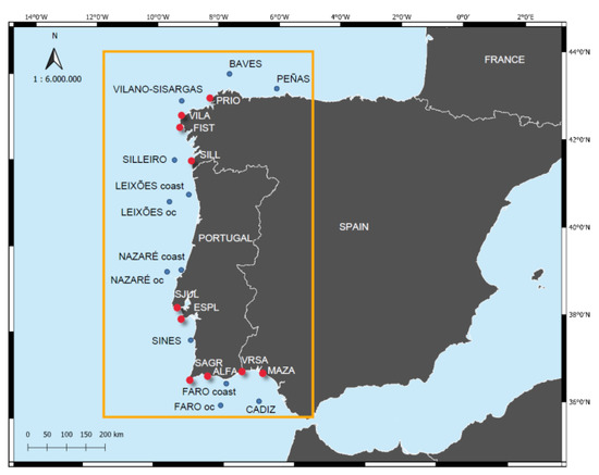
Figure 1.
Study area—Western Iberian Peninsula. Blue dots: wave buoy positions; red dots: high-frequency radars (HFR)’s site location; orange rectangle: the study area.
2.2. Data Sets
Wave parameters from broad-beam direction-finding CODAR SeaSonde HFR systems, buoy observations, and Sentinel-3 (S3) SA measurements are used in this study. The time window of the data sets is from January 2017 to December 2019 (36 months). All data sets were hourly time paired, and the SWH is the common parameter across the three different data sets. Besides the SWH, wave periods and wave directions are also used in the buoy vs. HFR wave data comparisons. The mean wave direction should not be confused with wave currents retrieved from the dominant first-order Bragg echoes.
Regarding the wave period analysis, CODAR Seasonde HFR systems output a period representing the centroid of the model being fitted to the second-order Doppler spectrum [18]. This variable is expected to be a more stable period estimator than the buoy dominant or peak period, which is a noisy estimator. The centroid represents a fit of the smooth spectral model to the entire wave spectrum. When comparing it against in situ observations, the SeaSonde’s centroid wave period (Tc) falls between the buoy’s dominant and average period [37]. Using the Tc from HFR is a relevant point to accurately interpret the results obtained from these HFR-derived period estimations. Concerning buoy observations, the peak and mean periods were used in our study.
2.2.1. In Situ Observations
Data from twelve wave buoys (blue dots in Figure 1) covering the study area, are used as reference ground truth for SWH comparison. In situ sensors can produce an accurate and continuous monitorization of coastal regions [7]. However, buoys’ observations time series suffer from inhomogeneity, due to differences in instrument type and location [38]. According to the manufacturer, instrumental buoy error was below 0.5% of measured SHW values after calibration. Table 1 shows the distance from shore and the wave data availability for each buoy during the study time window. The buoys used in the present study are located between 5 km (Sines) and 73 km (Leixões oceanic) offshore from the coast. The Portuguese Hydrographic Institute operates seven wave buoys (PT buoys in Table 1). The Puertos del Estado Spanish agency operates the other five buoys (SP buoys in Table 1). Hourly averaged measurements of SWH, wave period at spectral peak (or peak period—Tp), mean wave period (Tm), and wave directions are used. Gaps in wave data set, due to buoy maintenance periods.

Table 1.
Distance from shore and availability of buoy observations during a study time window (36 months). PT, Portuguese buoy; SP, spanish buoy.
2.2.2. Satellite Altimeters
SWH measured by SA is determined by tracking the slope of the leading edge of the return waveform to the nadir-looking altimeter [11]. Once the data is quality controlled, and sensor biases are removed, SWH errors in deep waters are comparable to buoy measurements [16,39]. Altimeter SWH data from the Sentinel-3 mission are used in this study. Sentinel-3A (S3A) was launched on 16 February 2016, and Sentinel-3B (S3B) on the 25 April 2018, orbiting in tandem mode with a repeat cycle of 27 days [8,13,40]. Among other sensors, these satellites host a SAR Radar Altimeter (SRAL) operating at Ku and C bands, which is the core instrument of the ocean surface topography, providing basic measurements of surface heights, wave heights, and sea wind speed [41,42]. The SRAL uses a linearly frequency-modulated pulse, and the primary frequency used for surface height measurements is the Ku-band (13.575 GHz). In comparison, the C-band frequency (5.41 GHz) is used for ionosphere corrections [10,41,42,43]. Along with SAR mode, S3 SA waveforms are also processed to generated pseudo-low-resolution mode (so-called PLRM) measurements similar to those produced by conventional altimeters [41,43]. The spatial resolution along the satellite track is approximately 7 km for 1 Hz measurements and ≈ 340 m for the 20 Hz [13,40]. This study uses SRAL data from S3A and S3B with 20 Hz sampling. To ensure the data sets’ quality and remove inaccurate observations, due to land contamination, only measurements with distances >5 km from the coast were used for buoys’ comparisons (>3 km for HFR RC comparison). Wave data is obtained from EUMETSAT (European Organization for the Exploitation of Meteorological Satellites) and downloaded from Copernicus Online Data Access (CODA) [44,45].
2.2.3. High Frequency Radars
HFR wave measurements have been collected by direction-finding CODAR SeaSonde HFR systems (red dots in Figure 1). The four long-range HFRs deployed in 2004, in the northern part of the study area (Galicia, Spain), are composed of two antennas each and use 4.86 MHz as working frequency [23,37]. Finisterre (FIST) and Silleiro (SILL) HFR sites are operated by Puertos del Estado, while Prior (PRIO) and Vilano (VILA) by INTECMAR. Mazagón (MAZA) is also a Spanish (SP) HFR site, but located in the south area of the Iberian Peninsula (see Figure 1). Puertos del Estado also operates MAZA station, and its working frequency is 13.5 MHz. Due to its geographic coverage area, MAZA HFR measures lower wave heights, so its frequency is higher than that of the Galicia HFR’s.
The Portuguese HFR stations (with operating frequencies between 12 and 13.5 MHz) are operated by the Portuguese Hydrographic Institute. S. Julião (SJUL) and Espichel (ESPL) HFR, the closest to Lisbon sites, are operational since 2010. Sagres (SAGR), Alfanzina (ALFA) and VRS António (VRSA) HFR, deployed along the south coast of Algarve, were installed between 2012–2016 by the TRADE project (http://www.tradehf.eu/; last accessed on 1 August 2020) [26]. TRADE HFR network’s primary goal is to improve port operations and safety of navigation from the Strait of Gibraltar, in Spain, to S. Vicente Cape, in Portugal, through 4 HFR sites (SAGR, ALFA, VRSA, and MAZA). SAGR HFR site also has a CODAR Tsunami detection software package installed [26]. The HFR data sets from FIST, VILA, PRIO, and SILL were provided by Puertos del Estado. The Portuguese Hydrographic Institute provided the remaining HFR site data sets (SJUL, ESPL, SAGR, ALFA, VRSA, and MAZA). Table 2 summarizes the standard information for each HFR, such as operation frequency, RC resolution (RCr), number of available RCs with wave data availability, the coverage area for wave parameters, and coastline sector from which the wave data is extracted. The coastline sector, or coastline limits, define the coverage area according to the shoreline and the open ocean surrounding the radar.
Table 2.
HFR sites information regarding wave data acquisition. Standard information of each HFR: Operation frequency, range cells (RC) resolution, number of available RC, coverage area and coastline sector.
In the HFR systems, wave data are collected from circular or annular cells (RC) arranged from the antenna [18,31,45]. Each of these RC has a width with a specific distance counting from the HFR antenna position, corresponding to the RC spatial resolution [28,37]. The RCr will be the same for all the HFR RCs, but it will vary from site to site, depending on the frequency and type of system being used. The homogeneity of the ocean spectrum is assumed over each HFR RC [18,19,36,37].
The HFR coverage area for the wave data acquisition is shown in Figure 2. For each HFR are represented the individual RCs, as well as the closest buoys. In the lowest frequency HFR sites, such as PRIO, VILA, SILL, and FIST, the RCr is higher than the remaining HFR, which leads to a larger width for these HFR RC (red circles). The amount of wave data is, in general, relatively low near the shoreline, due to the range and architecture of the HFR antennas [20,37,46]. The wave data availability also tends to decrease as the HFR antenna’s distance increases [20,37]. Figure 3 shows the wave data availability of individual HFR RCs concerning the distance to the coast. The availability for each HFR is represented in two lines: the first one corresponds to the total availability of RC wave data (dashed lines). The second is the wave data acquired by each RC without radar nulls (solid lines). Low-frequency sites (4.86 MHz) are graphically depicted in Figure 3a and the higher frequency sites (12–13.5 MHz) in Figure 3b.
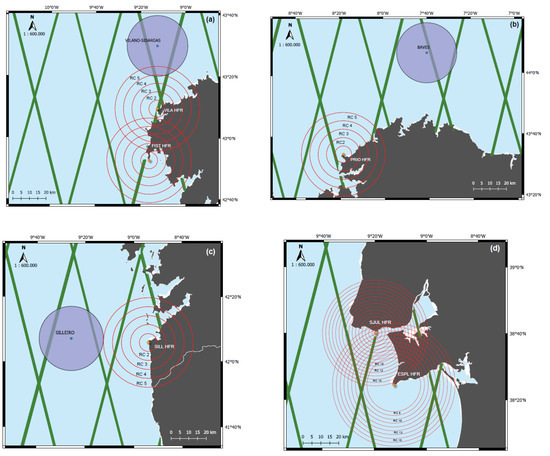
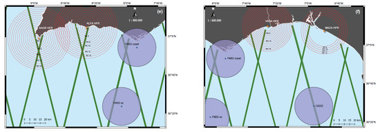
Figure 2.
Wave data HFR coverage area. (a) VILA and FIST HFRs (RCr = 5.1 km); (b) PRIO HFR (RCr = 5.1 km); (c) SILL HFR (RCr = 5.1 km); (d) SJUL HFR (RCr = 1.85 km) and ESPL HFR (RCr = 2.15 km); (e) SAGR and ALFA HFRs (RCr = 1.85 km) and (f) VRSA HFR (RCr = 1.51 km) and MAZA HFR (RCr = 1.67 km). Red circles: RCs; blue dots: wave buoy locations; green lines: Sentinel-3 tracks and blue circles: 10 NM area for in situ and SA comparisons.
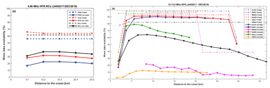
Figure 3.
Overview of captured and useful HFR wave data per RC against distance from the coast (36-months period data sets). (a) 4.86 MHz HFR stations (Blue line: PRIO; Red line: VILA; Black line: SILL) and (b) 12–13.5 MHz HFR stations (black line: ESPL; blue line: ALFA; red line: SAGR; pink line: MAZA; green line: SJUL; orange line: VRSA). Dashed lines represent the total availability, and the solid lines the availability without radar nulls. Dots and circle markers represent each RC.
Galician HFR sites can measure high SWH values (SWH > 20 m), due to their lower operating frequency [20]. During the 36-months, these three HFR sites could only acquire less than 40% of useful wave data (no nulls). In Figure 3a, the HFR trend to capture less quantity of wave data, too close and too far from the coast, is present. For the remaining HFR (12–13.5 MHz), depicted in Figure 3b, the amount of useful data is quite different from that presented in Galicia. The gap of HFR wave data near the shoreline is evident, as well as in the farthest RCs, where the data availability decreases abruptly. ALFA and SAGR are the sites with the highest percentage of useful data (no nulls > 85%). The SJUL HFR presents wave data availability between 60% and 80%. ESPL and VRSA sites, on the other hand, show a consistent but lower quantity of data, with 60% decreasing to 15% and 38%, respectively. The MAZA HFR is the site that captured the lowest percentage of useful wave data (no nulls < 20%).
The lower frequency HFR systems provide 30-min sampling rate wave data, subsequently averaged at 60-min intervals, ensuring temporal resolution consistency. The higher frequency HFR systems provide 10-min wave data, also further averaged at hourly intervals. Each HFR site’s operational frequency determines the maximum and minimum wave height measured by the system. The lower the frequency, the higher the wave height that can be measured [18,26]. Waves with heights up to 20 m can be measured by the 4.86 MHz frequency HFR [18]. Working frequencies of 12–13 MHz, theoretically, can measure a minimum (maximum) wave height of 1 m (8 meters) [37]. If the waves are sufficiently energetic, HFR systems will provide wave parameter estimations from second-order spectra. The wave parameters are obtained directly by the SeaSonde CODAR HFR proprietary software, which processes 30-min of the received signal into Doppler cross spectra and saved in Cross Spectra Short time (CSS) files [23,28,47]. A pre-established sampling period, defined by a specific number of CSS files, calculates the directional wave spectrum and retrieves the wave parameters [47,48]. In the extracted files from the HFR software, the minimum and the maximum wave period were fixed to 5 s and 17 s, following CODAR recommendations [47]. Hourly measurements of SWH, Tc, and wave direction values are used to HFR-buoy comparisons. Data from FIST HFR were not available for the study time window (2017–2019), since this station has suffered a long and severe break-down. VRSA and MAZA HFR were operating during the same period, but the amount of available data is low, as will be shown further. Other occasional gaps in the data are due to HFR system maintenance periods (see Figure 4).
Figure 4.
Availability of in situ and matchable HFR wave data during the study period (36 months). (a) PRIO HFR (RC-5)/Baves buoy; (b) VILA HFR (RC-5)/Villano-Sisargas buoy; (c) SILL HFR (RC-5)/Silleiro buoy, and (d) ALFA HFR (RC-15)/Faro coastal buoy. Blue dashed lines with dot markers: wave buoy data availability; Grey lines with triangle markers: total HFR wave data availability; red lines with circle markers: HFR wave data availability after excluding the nulls and spurious values.
2.3. Data Analysis Methods
To assess the ability of the western Iberian Peninsula HFR systems in retrieving wave data, a comparison between HFR-buoy observations is performed. Previous comparisons with wave buoys have shown a positive contribution of HFR systems in retrieving reliable wave data [25,45,49,50]. The proximity of wave buoys to the HFR site, or closest RCs, was considered for the HFR-buoy wave data comparison. Table 3 describes the distance between buoys and the HFR sites. Only the buoys in line-of-sight with the HFR sites are presented.
Table 3.
Distance between HFR stations and buoys (km). Grey cells: HFR-buoy with wave data observation pairs.
HFR wave parameters from all individual RCs are analyzed. The furthermost distance at which wave data are available from the HFR origin sites is 25.5 km (PRIO, VILA, SILL HFR-RC5), 18.5 km (SJUL-RC10), 34.4 km (ESPL-RC16), 27.75 km (SAGR-RC15); 29.6 km (ALFA-RC16), 22.65 km (VRSA-RC15) and 20 km (MAZA-RC12) (see Table 2). The outermost HFR RC, which is closer to a buoy position, and in line-of-sight with the HFR transmission antenna, is selected. Thus, only four HFR-buoy sensor pairs are analyzed, due to the buoys’ geographical distance to the respective HFR RC. In other words, since the Villano-Sisargas buoy is 37 km from shore, we can derive that remote-sensed wave estimations are representative of a 12 km region from the buoy (distance between RC5 and buoy location), setting up the context for the discussion results. The oceanographic conditions around each buoy do not vary much for a 20–30 km area in the buoy position’s vicinities. Unless if the buoy is in very shallow waters, which is not the case (all buoys depths > 50 m). Following the same criterion, the HFR-buoy comparisons were made for SILL (RC5–20 km apart from Silleiro buoy), ALFA (RC15–22 km apart from FARO coastal buoy), and PRIO (RC−5–57.5 km apart from Baves buoy). Summarizing, the HFR-buoy analysis is performed between PRIO/Baves, VILA/Villano-Sisargas, SILL/Silleiro, and ALFA/Faro coastal (grey cells in Table 3). For the remaining HFR sites, the HFR-buoy comparison was not possible to be conducted, due to its higher distance from buoys, or because the amount of wave data from HFR sites, such as MAZA and VRSA, was not enough or paired with buoy observations. FIST HFR wave data will not be used in the present study, due to the previously reported problems related to the site’s inoperational period.
In the SeaSonde CODAR HFR systems, wave data are retrieved from single RCs, and the acquisition depends on the sea state characteristics throughout the RC itself. Therefore, the percentage of data recorded that can be extracted might differ among RCs. In the validation of HFR wave parameters, radar nulls and other spurious values detected during the datasets screening are excluded. The screening of the HFR datasets was carried out by comparing it with SWH data with the hourly buoys time series. After the preliminary comparison of the datasets, RMSE > 3 σ (standard deviation) was considered a spurious value, and the respective HFR-buoy pair observation was removed. The comparison of the datasets was made, once more, without spurious values and the statistics achieved. Figure 4 and Figure 5 show the availability of HFR wave data during the 36-month study time window. The wave data availability for HFR-buoy comparisons is represented in Figure 4 through buoy availability, HFR total availability, and HFR wave data without nulls or spurious values. As can be seen, the availability of wave data in HFR without nulls or spurious values (red lines with circle markers in Figure 4 plots) is always lower than buoy or HFR total wave measurement values. ALFA HFR (Figure 4d) show more consistency in the wave data’s availability through the entire 36 months period. As stated before, ALFA is the HFR site with more useful wave data (no radar nulls) (Figure 3b). For the Galician HFR, the gaps in the HFR sites’ operability are also noted. PRIO HFR has wave data gaps between February to December 2017 and August to December 2018 (Figure 4a). The wave data gaps for the VILA HFR site are from January to May and from August to November in 2017. For March and between June-August 2019, VILA HFR also does not have available wave data (Figure 4b). SILL HFR has wave data gaps between October-November 2017 and August to December 2019 (Figure 4c). These wave data gaps are due to malfunctioning or HFR equipment maintenance periods and justified the wave data availably <40% of the Galician HFR sites (Figure 3a).
Figure 5.
Availability of HFR wave data for the 12–13.5 MHz sites (36 months). Blue line: SJUL (RC10); blue dashed line: SJUL (no nulls); red line: SAGR (RC15); red dashed line: SAGR (no nulls); black line: ESPL (RC15); black dashed line: ESPL (no nulls); green line: VRSA (RC15); green dashed line: VRSA (no nulls); orange line: MAZA (RC12); orange dashed line: MAZA (no nulls).
Figure 5 shows the wave data availability for the 12–13.5 MHz HFR sites. ALFA HFR (13.5 MHz) was already presented in Figure 4d. After discarding the nulls and spurious values, VRSA and MAZA HFR sites have shown to have the lowest availability of wave data, which can be partially justified by these sites’ location in a sheltered area in the south of the Iberian Peninsula. In these coastal areas, the annual mean wave height value is lower than 2 m. The second-order spectra echoes can be very weak for lower sea states, and spurious features in the spectrum can contaminate the wave parameter estimation [36]. ESPL HFR shows low consistency on the quantity of available wave data (no nulls), and SJUL and SAGR are the sites with the higher wave data availability.
Due to the almost no overlapping between HFR systems and buoy observation, with only four HFR-buoy pairs as previously mentioned, SA SWH measurements will be compared with HFR for each RC to evaluate the HFR skills in measuring SWH. Buoy observations are used as ground truth to validate the SRAL SWH measurements for the HFR-SRAL comparison. Direct comparison with in situ observations have already shown the overall improved performance of the SRAL, compared with previous SA missions in Europe [8,9,13]. Due to the smaller ground footprint and higher spatial resolution of SRAL observations, the 20 Hz measurements from SRAL are expected to be overall more accurate in coastal areas than conventional nadir altimetry [14]. Following this assumption, SRAL SWH measurements are compared with in situ observations from 12 coastal wave buoys. A 10 nm (≈18.52 km) circular area from the buoy position was set (blue circles in Figure 2), and only the SRAL measurements inside these areas are compared. Each SRAL track (green lines in Figure 2) inside these 10 nm circular areas recorded several measurements during a few seconds. Thus, each track’s mean value has been computed for the satellite passage time inside each circular area. The satellite passage time over the study area, and consequently in the circular buoy areas, is between 10:51–11:14 UTC and 21:52–22:14 UTC, depending on whether they are ascending or descending satellite passages and from S3A or S3B [43]. The comparison time is related to buoy hourly observations, for these specific cases, 11:00 UTC and 22:00 UTC, regarding the satellite passage time.
As the SRAL SWH measurements overlap all the different HFR RC, an HFR–SRAL comparison can evaluate the HFR performance to retrieve SWH as the HFR site’s distance increases. For the SWH HFR–SRAL comparison, only the SRAL measurements inside each HFR RC are used. Figure 6 presents an exemplificative scheme of the SRAL track inside SILL HFR RC (Figure 6a) and VRSA HFR RC (Figure 6b). The same criteria were used for each HFR. Considering that the amount of captured wave data can vary for each RC, due to the sea state, the SWH is computed for individual RC. As described before for HFR-buoy comparisons, an averaged SWH value of every satellite passage inside respective HFR RC is achieved and then compared with the equivalent time HFR derived SWH. The following statistics are used in the comparison of buoys, HFR, and SRAL data sets:
where given observation pairs from different data sets are represented by , b is the buoy observations, and s the SRAL measurements (or the HFR RC wave data). N is the number of observation pairs, and an overbar represents the mean value. R is the linear correlation factor, SI the scatter index, and RMSE the root-mean-squared error from each correlation (R) of the data sets.
Figure 6.
Sentinel-3 tracks over HFR RC. Exemplificative schema for (a) SILL HFR and (b) VRSA HFR. Green tracks: Sentinel-3 tracks with SRAL measurements; red circles: RC; blue dot: Silleiro buoy.
3. Results
3.1. HFR vs. Buoy
Wave height comparisons of HFR-buoy measurements have previously presented HFR consistent performances in retrieving reliable wave information [3,19,35,37,51]. However, a slight overestimation by the HFR systems is usually reported. The HFR RC geographically closest to each buoy position has been selected for the HFR-buoy wave data comparison. Hourly measurements at selected RC are compared with the buoys wave parameters (SWH, wave period, and wave direction).
The Emma storm, a winter storm that has affected Western Europe, was analyzed to evaluate the HFR systems’ ability to capture extreme wave events. The storm was formed on 26 February 2018 and dissipated on 5 March 2018. Although weakened to a post-extratropical cyclone, it brought severe weather in terms of heavy rain, high waves, damaging gusts, small tornados, and storm surges with subsequent coastal flooding.
3.1.1. Significant Wave Height
The comparison between HFR-buoy SWH observations is shown in the density scatter plots in Figure 7. The correlation between the two SWH data sets, during the 36 months, is above 0.84, except for the ALFA HFR site (Figure 7d), with R = 0.66. The RMSE is between 0.89 m and 1.18 m., and the negative bias indicates a slight overestimation of the SWH by the HFR sites. This reported overestimation can be seen in ALFA HFR (Figure 7d). On the other hand, the slope value derived from the scatter plots’ best linear fit is very close to 1, except for the ALFA site (slope = 1.26). ALFA HFR site has the highest number of valid observations pairs (N = 21979) during the study time window. The correlation of 0.66 can be partially justified by increasing the valid observations, which can deteriorate the statistic metrics’ performance. To achieve if the statistic metrics present some seasonality, the SWH datasets were divided into four seasons (DJF—December, January, and February; MAM—March, April, and May; JJA—June, July, and August, and SON—September, October, and November). The results are presented in the scatter plots of Figure A1 and Figure A2 in Appendix A. The density scatter plots depicted in Figure 7 result from comparing the HFR-buoy SWH observations across 36 months. Table A1, Table A2 and Table A3 in Appendix A presents individual monthly statistic metrics for the HFR-buoy SWH comparison.
Figure 7.
Comparisons between buoy and HFR SWH (density scatter plots). Statistics metrics are gathered on the right bottom side. N represents the number of coincident hourly observations, and the red dashed lines are the best linear fit of the scatter plots. Density scatter plot: (a) Baves buoy vs. PRIO HFR (RC5); (b) Villano-Sisargas buoy vs. VILA HFR (RC5); (c) Silleiro buoy vs. SILL HFR (RC5) and (d) Faro coastal buoy vs. ALFA HFR (RC15). The colored bar represents the density of the scatter plots.
The availability of buoy and HFR wave data are very different, as shown in Figure 4. For the graphic presentation of the study, one month was chosen to serve as an example. The choice followed two criteria. The availability of the wave data between the data sets was the first criterion. Looking for Figure 4 and Figure 5, and for the monthly statistic metrics (Table A1, Table A2 and Table A3), March 2018 was the month that, among buoys and HFR sites, had the higher observation pairs, availability of wave data (no nulls), and a higher correlation between the data sets. It was also the period when Emma’s storm affected Europe. Between 28 February and 2 March 2018, storm Emma hit the Iberian Peninsula, severely damaging. One of this study’s goals is to evaluate the HFR’s ability to detect extreme wave events, so it seems to the authors as the right month choice.
In Figure 8, HFR-buoy SWH comparisons are displayed for March 2018 through time series, scatter, and QQ plots. The preliminary analysis of these plots shows the ability of HFR to capture extreme wave height events. The time series plots (Figure 8(a1,b1,c1,d1)) show a good agreement between the two data sets. Although, HFR seems to slightly overestimate the SWH when compared with the same period of buoy observations. A scatter plot analysis is used to determine the correlation between the data sets (Figure 8(a2,b2,c2,d2)). The statistic metrics for March 2018 present a correlation between 0.84 and 0.92. These values are higher than the overall correlation for the three years of observations (Figure 7). On the other hand, the monthly values presented in Appendix A for the HFR-buoy SWH comparison exceed the overall R (0.84, 0.87, 0.85, 0.66), in some cases. In March 2018 statistics results, the RMSE varies between 0.69 m (ALFA) and 1.18 m (PRIO). The negative bias (−0.06 m to −0.37 m) indicates an overestimation of the SWH by HFR sites.
Figure 8.
One-month comparison of HFR SWH against in situ observations—March 2018 (Emma Storm). (a) PRIO HFR vs. Baves buoy; (b) VILA HFR vs. Villano-Sisargas buoy; (c) SILL HFR vs. Silleiro buoy and (d) ALFA HFR vs. Faro coastal buoy. (a1,b1,c1,d1) Time series plots (blue line: buoy observations, red line: HFR derived SWH; black crosses: SRAL measurements); (a2,b2,c2,d2) Scatter plots (blue dots: observation pairs, red dashed line: best linear fit); (a3,b3,c3,d3) QQ-plots (black dots: buoy against HFR quantiles; black line: quantiles normal distribution; red dashed line: quantiles distribution and blue filled dots: 90, 99 and 99.9 quantiles). Statistics metrics of the comparison between the buoy and HFR SWH for March 2018 are gathered on the right bottom side of the scatter plots.
Figure 8(a3,b3,c3,d3) depict the HFR-buoy SWH QQ-plots. The QQ-plots confirm the overestimation mentioned above of the HFR SWH measurements, particularly for high-sea states and wave height events above the 90th percentile. Extreme wave events occur between the 90th and the 99th percentiles [34,51]. Through the analysis of the QQ-plots, at Galicia (Algarve) region, a wave height above 6 m (4 m) can be considered an extreme event. On 1 March 2018, Faro coastal buoy captured SWH = 6.5 m. The ALFA HFR site also captured this value during the same period (Figure 8(d1)). The black crosses, shown in the time series plots (Figure 8(a1,b1,c1,d1)), represents the SRAL SWH observations, where the high correlation with in situ observations is clear.
Regarding the NW area of the Iberian Peninsula, covered by three of the HFR sites (Figure 8: a-PRIO; b-VILA and c-SILL), the effects of the Emma storm were felt later, on 11 March. Values above 8 m of SWH were captured by Villano-Sisargas and Silleiro buoys. These extreme wave height values correspond to swell, originated by the storm passage between the Azores archipelago and the Iberian Peninsula. SILL and VILA HFR sites also captured similar values (slightly overestimated) for March 2018. PRIO HFR and Baves buoy are geographically located in a more sheltered area, and for that matter, measured lower values. In March 2018, all three sites registered another extreme wave height event (on the 24th), with values between 9–10 m. These plots further confirm a slight underestimation of the lowest SWH values by the HFR sites, also depicted in the time series graphics.
3.1.2. Wave Period
In the SeaSonde CODAR HFR systems, the wave period is considerably more sensitive to noise in the radar backscatter than SWH, particularly in low sea states [20,36]. As discussed in previous sections, buoy and HFR provide different outputs for wave periods. HFR systems retrieve a period representing the centroid of the model fitted to the spectral data (Tc—centroid period). At the same time, buoy provides Tp and Tm [18,36]. Tc can be assumed as a stable estimator as Tm, while being more stable than Tp, which is noisier [37]. Theoretically, Tc should be between Tm and Tp [19,36,37]. The HFR Tc was compared to the Tm, and Tp outputs from the buoys (where available) to achieve which buoy period correlated best with the CODAR SeaSonde wave period. As Tp is always longer than the Tm from buoys, it sometimes represents swell when the swell is present. However, its utility as a precise parameter is cast in doubt by its significant statistical uncertainties. Figure 9 displays the different wave periods comparison, through time-series of one exemplificative month (March 2018).
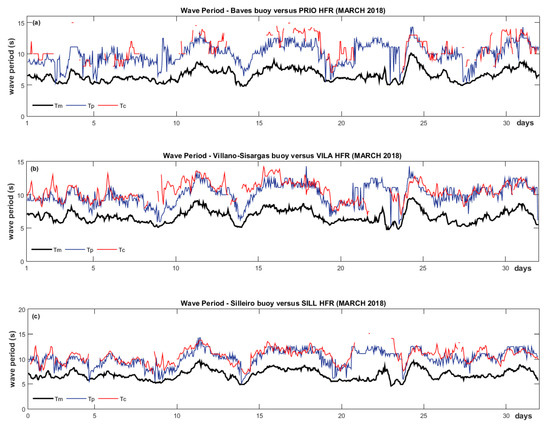
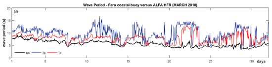
Figure 9.
Wave period time series for March 2018. (a) PRIO/Baves buoy; (b) VILA/Villano-Sisargas buoy; (c) SILL/Silleiro and (d) ALFA/Faro coastal buoy. Black: mean wave period (Tm) from buoy; blue: peak period (Tp) from buoy and red: centroid period (Tc) from HFR.
In all the time series plots (Figure 9a–d), Tm corresponds to the most stable estimator and Tp to the noisiest. In Figure 9d, which represents ALFA HFR Tc and Faro coastal buoy Tm and Tp during March 2018, Tc estimates fell between Tm and Tp, in line with the previous reports [19,36,37]. For the remaining HFR sites (PRIO, VILA, and SILL—Figure 9a–c, respectively), Tc revealed to be as noisier as Tp. However, the overall correlation achieved between Tc and the buoy periods shows a better agreement with Tp. The comparison between Tc and buoys’ periods (Tm and Tp) for the HFR-buoy pairs was achieved for the 36-month period, and the statistics metrics are summarized in Table 4.
Table 4.
Comparisons between buoy wave periods (Tp and Tm) and HFR Tc (36-months period). Statistics metrics: Correlation coefficient (R), RMSE, bias, SI, and slope. N corresponds to HFR & Buoy SWH observation pairs (hourly observations).
The HFR-buoy periods’ comparisons present RMSE values between 1.90 s to 3.09 s for Tp and from 3.26 s to 4.71 s for Tm. Negative bias values (Tc > Tm/Tp) indicated overestimation by the HFR site, while positive ones (Tc < Tm/Tp) underestimation. The scatter plots of the wave period comparison are presented in Appendix A—Figure A3. In these plots, the under/overestimation of the wave period can be seen throughout each linear regression slope. The overestimation of the Tc by the HFR is clearly noted, when compared to the Tm (Figure A3a,c,e,g). On the other hand, when Tc is compared with Tp, the results indicate a slight underestimation of the Tc by the HFR system (Figure A3b,d,h). The R varies between 0.46–0.68 and 0.52–0.65 for Tm and Tp, respectively.
3.1.3. Wave Direction
Wave direction is obtained from the 2D energy density wave spectrum and is strongly influenced by the wave height [20]. Spurious contributions to the directional spectra, such as radio interferences, might contaminate the radar backscatter signal and eventually lead to inaccurate wave direction measurements by the HFR systems [34,46,50]. These directional biases can also be enhanced in low sea states (SWH < 2 m) [36].
The scatter plots depicted in Figure 10 show the relation between SWH and wave direction measurements for buoys (Figure 10a,c,e,g) and HFR closest sites (Figure 10b,d,f,h). Due to the coastline configuration, a coastline sector, or coastline limits are defined for each HFR site. According to the shoreline and the open ocean surrounding the radar, this coastline sector corresponds to the HFR coverage area. The information gap in the scatter plots in Figure 10 corresponds to the area not covered by the HFR coastline sector, where no wave data is acquired.
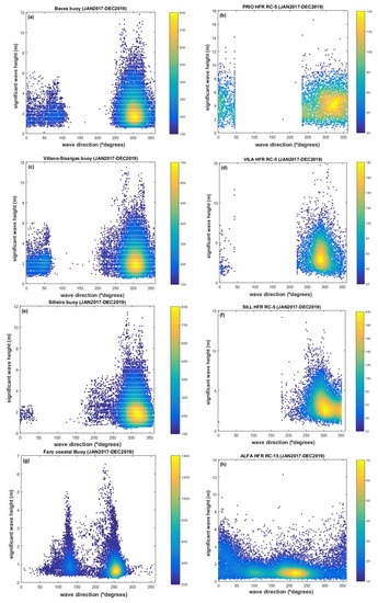
Figure 10.
Density scatter plots of SWH (m) vs. wave direction (JAN2017-DEC2019). (a) Baves Buoy; (b) PRIO HFR; (c) Villano-Sisargas buoy; (d) VILA HFR; (e) Silleiro Buoy; (f) SILL HFR; (g) Faro coastal buoy and (h) ALFA HFR. (a,c,e,g) in situ sensors and (b,d,f,h) HFR wave data. Central colored bar legend represents the density of both scatter plots.
In the scatter plots representative of the Galician buoys (Figure 10a,c,e) and HFR (Figure 10b,d,f) wave direction, an NW-NNW (300–340) predominant incoming wave direction can be identified. This spatial distribution is influenced by the Galicia coastline morphology and by the periodic passage of frontal systems originated in the North Atlantic Ocean [34]. On the other hand, Faro coastal buoy (Figure 10g) and ALFA HFR (Figure 10h) revealed wave directions, with predominant sectors from SW-WSW (220–250) and residual waves coming from ESE-SE (110–140). The spatial distribution for Faro coastal buoy and ALFA HFR is following the Algarve region’s coastline morphology and the natural sheltered conditions of this area.
The time series depicted in Figure 11 shows the distribution of the HFR-buoy wave direction for March 2018. Despite the information gaps in the time series, the wave direction patterns are similar between buoy and HFR. In Figure 11d, the ALFA HFR wave direction is more scattered from 20 March till the end of the month. According to the SWH time-series plots (Figure 8d), this period corresponds to lower sea states, with SWH < 2 m.
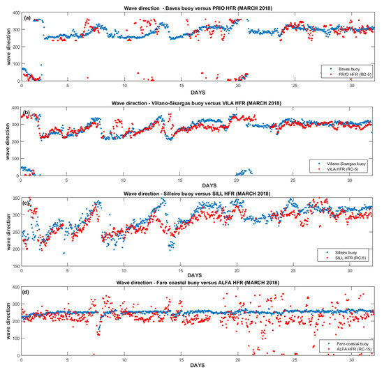
Figure 11.
Wave direction time series buoy vs. HFR (March 2018). (a) PRIO/Baves buoy; (b) VILA/Villano-Sisargas buoy; (c) SILL/Silleiro and (d) ALFA/Faro coastal buoy. Blue dots: buoy wave direction and red dots: HFR wave direction.
3.2. Satellite Altimeter vs. Buoy
Statistics metrics of SRAL-buoy comparisons are summarized in Table 5. The overall R > 0.89 indicates that SRAL observations can accurately retrieve SWH near the coast. In coastal areas, SA data quality tends to deteriorate, due to land contamination of the altimeter’s footprint. Nevertheless, the correlation coefficient is above 0.94. An exception was made for the Sines buoy, where R = 0.91 and Cádiz buoy with R = 0.89. The RMSE of SRAL measurements varies between 0.17 m and 0.65 m. As expected, SWH values retrieved from SRAL tend to be less accurate nearshore. The less accurate SRAL SWH measurements were achieved for Sines buoy position, the closest to shoreline buoy (≈5 km). At this location, also the bias presents the higher value (bias = −0.45 m), showing a slight overestimation by the SRAL. The regression slope approaching the 1:1 relation and the RMSE values presented in Table 5 indicate a good performance of the SRAL for coastal zones. The small number of SRAL-buoy observations used to compute the statistic metrics are related to the S3 revisit time inside the buoy 10 nm circular area. The SRAL-buoy observation pairs have increased after the S3B launch and the respective availability of data since December 2018. Moreover, the number of SRAL-buoy paired observations is also larger than related studies [12], which had presented N = 40/47 for ENVISAT SA measurements during nine years (2002–2012), in six particular zones.
Table 5.
Comparisons between SRAL and buoy SWH measurements. Statistics metrics: Correlation coefficient (R), RMSE, bias, SI, and slope. N corresponds to SRAL-buoy SWH observation pairs. SP: Spanish buoys and PT: Portuguese buoys.
3.3. HFR vs. Satellite Altimeter
Bearing in mind that the correlation coefficient between SRAL and the in situ wave measurements is high (R > 0.89), SRAL measurements are from here onwards taken as the reference through the following and final analysis. Any differences between SRAL and HFR SWH data sets are, therefore, accounted for as errors in the HFR measurements. This assumption led to the fact that buoy observations are restricted to a geographic position (point), and HFR wave data reference to a circular sector (RC). The gap of coincident in situ information with each HFR RC is also a contributing factor for using SRAL measurements as a matchable data set, exclusively in this analysis (HFR-SRAL).
The HFR-SRAL comparison was conducted, and the statistic metrics are summarized in Table A4, Table A5 and Table A6, in Appendix A. This analysis allows the evaluation of how SWH measurements vary with the distance to the coast. The correlation coefficient and RMSE values for the PRIO, VILA, and SILL HFR sites are presented in Figure 12. The correlation within each HFR RC, slightly decreases as the distance to the coast increases. The agreement of the measured SWH data sets is high, with correlations between 0.86–0.99. RMSE values vary in the inverse proportion with the R, as the distance to the coast increases. The best correlation between HFR-SRAL is achieved at RC4 (≈ 20 km from the coast), for all Galician sites. The negative bias indicates an SWH overestimation by the HFR. The RMSE for RC4 is 0.57 m, 0.53 m, and 0.81 m, for the PRIO, VILA, and SILL sites, respectively.
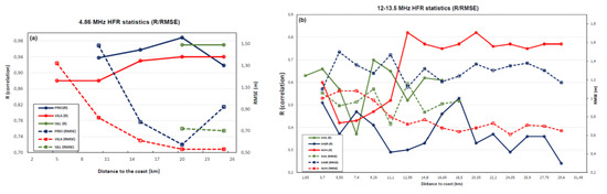
Figure 12.
Root-mean-squared error (RMSE) and correlation (R) between HFR-SRAL SWH measurements as a function of distance to coast (km). (a) 4.86 MHz HFR sites (red: VILA; blue: PRIO and green: SILL); (b) 12–13.5 MHz HFR sites (red: ALFA; blue: SAGR and green: SJUL). Dashed lines: RMSE (m) and solid lines: R.
The 12–13.5 MHz HFR sites present results quite different from those achieved for the Galician HFR. The correlation and RMSE values for SJUL, SAGR, and ALFA HFR sites are presented in Figure 12b, according to Table A5 (Appendix A). An overall negative bias was achieved, forwarding for an overestimation of the SWH by the HFR. SJUL site presents a correlation between 0.61 and 0.70. The better agreement was detected in RC6 (11 km from the coast) with R = 0.70, bias = −0.23 m and RMSE = 0.72 m. The SAGR HFR show inconsistent results with RMSE values above 1.10 m. The correlation achieved was low, varying from 0.24 to 0.53 (RC10). ALFA site presents better results, particularly from RC7 to RC16. Statistic metrics vary from 0.75 to 0.82 in correlation, −0.14 m to −0.40 m in bias, and from 0.61 m to 0.77 m for the RMSE.
4. Discussion
The present study evaluates a 36-months long time series of HFR wave data. To our knowledge, only a few studies so far have considered time series of HFR wave data as long as the one presented here [9,34,36,37,38,46,51,52,53,54]. Even fewer studies have incorporated SA and HFR wave parameter comparisons in the same type of analysis [3,9,33,37]. In this study, an evaluation of SeaSonde CODAR HFR systems skills on retrieving wave data at the western Iberian Peninsula is carried out by comparing with SRAL and in situ wave measurements.
Nowadays, HFR systems are a valid instrument for simultaneously measuring and monitoring surface currents and wave parameters [20,36,50,52]. The measurement of surface currents by HFR systems is, in fact, the main focus of most of the available literature [32,54,55,56,57]. Nevertheless, HFR systems can also measure the wave spectrum and retrieve wave parameters [18,20,27,37]. As surface currents are obtained from the first-order Doppler spectrum of the radar, they can be measured over a broader range of sea states than waves. On the other hand, wave parameters are derived from the lower amplitude second-order radar echoes [21]. The inversion of the second-order part of the backscatter spectrum and the validation of HFR wave parameter measurements are still active research areas [23,34,35,36].
Wave measurements from SA are good alternatives for monitoring coastal areas, due to their global coverage [3,8,9]. However, SA tends to slightly overestimate the SWH compared with in situ observations, particularly in coastal areas [8,9,10,11,12,13]. While in open ocean SA data are of considerably good quality, the accuracy tends to deteriorate at nearshore areas, mainly due to land contamination in the altimeter footprint [8,9,10,11,12,13,14,15,16,17]. Theoretically, and regarding numerical models’ predictions in literature [8,9,10,11,13,15,16,17], SA accuracy is expected to decrease for observations progressively closer to the coast [11,12,13,15,16,17]. Thus, correlations with coastal buoy observations are characterized by an inverse relation with distance from the coast [13]. Previous works argued that the correlation between SA and buoy measurements increases for distances further than 10 km from the coastline [10,12].
In this study, SRAL measurements from S3A and S3B are validated through buoy observations before being compared with HFR SWH data. Overall a good performance of SRAL measurements is noted through the West Iberian Peninsula coastal areas, with correlations for SWH measurements above 0.89, RMSE between 0.17 m to 0.42 m, and a regression slope range of 0.92–1.09. Even within 10 km off the coast, as in Faro and Nazaré buoys, the results revealed a higher agreement, with R varying between 0.95–0.98, biases from −0.05 m to 0.19 m, mean SI of 0.15, and RMSE between 0.19 m and 0.33 m, respectively. These results followed recent works that underlined the good performance of SRAL measurements beyond 5 km from the shore, after comparisons with buoy observations [10,13,58,59]. When comparing SRAL SWH data with U.S. National Data Buoy Center (NDBC) buoys, located between 5–25 km off the coast, results showed RMSE values of 0.30/0.31 m for S3A/S3B [58]. Even when compared with similar SA sensors, such as Janson-2 or CryoSat-2, S3A had achieved better performances within 10 km of the coast (R = 0.91; bias = 0.17 m; SI = 0.33; RMSE = 0.40 m) [8]. The SRAL performance over coastal areas and the ability to retrieve SWH beyond 5 km from the coast were demonstrated. Meanwhile, the first steps in using S3 SRAL to retrieve water surface elevation over rivers are being taken, with very satisfactory results over Chinese rivers (RMSE: 0.12 m to 0.9 m) [59].
The co-location of radars and buoys for HFR wave data validation is ideal, but not always possible. In situ sensors give point observations, while CODAR SeaSonde HFR systems derive wave parameters from a least-squares fitting technique applied between second-order spectra and a Pierson-Moskowitz model. The homogeneity of the ocean spectrum is assumed over the HFR RC [18,19,36,37]. Direction-finding systems like CODAR SeaSonde HFR, require the validation of this assumption, while beam-forming systems, like WERA HFR, do not [52]. It is certain that for HFR-buoy comparison, the inexistence of overlap between the buoy and HFR RC data sets was the motive that contributes the most for the relatively lower correlation of 0.66 in the ALFA site. The differences and the low correlations between HFR-buoy can partially be explained by assuming the spectrum homogeneity in the entire RC. This hypothesis can be erroneously assumed on the ground, due to relevant bathymetric variations in coastal areas [34,37].
Coastal effects can also lead to local variations in wave fields, making it even harder the HFR-buoy comparisons [34]. Another possible explanation is because the CODAR SeaSonde software assumes infinite water depth [34,60,61]. The shallow water effects can become significant for lower water depths, causing an impact on radar sea surface echo, increasing the second-order spectral energy, and decreasing the saturation limit on wave height as water depth decreases [61]. For a radar transmit frequency of 5 MHz, the depth at which shallow water creates an effect is 35 m [34]. Other studies revealed that for 13 MHz transmitting frequency radar, shallow water effects become significant in water depths <30 m [60]. Due to the Iberian coastline morphology and its associated bathymetry, all the buoys are positioned in depths >50 m. All the RCs selected to be compared with in situ observations are the RCs furthermost from the HFR origin. These RCs are located at 25.5 km (Galician sites) and 27.75 km (ALFA site) from the shoreline, at depths >50 m, far enough to ensure the deep-water assumption.
Despite these limitations, HFR and buoy observations appear to capture similar wave features and temporal variability. For HFR-buoy SWH comparison, a general overestimation of the SWH by the HFR has been noted. All the results revealed negative bias values. The correlation and the RMSE of the observation pairs overall (36-months) had reached to 0.66–0.87 and 0.89–1.18 m, respectively. Concerning individual monthly evaluations, higher correlations are achieved, such as December 2017 (PRIO), January 2019 (VILA), and March 2018 (SILL and ALFA) (see Table A1, Table A2 and Table A3 in Appendix A). This fact is related to the availability of HFR wave data through different seasons and sea states. Even so, the ALFA HFR presented the less accurate results and a higher overestimation of SWH, easily noted through the spreading of the observation pairs in the scatter plots (Figure 7d), revealing a SI of 0.84. To evaluate if the previous statistic metrics present some seasonality, the datasets were divided into four seasons (DJF/MAM/JJA/SON). JJA in all the 4 HFR-buoy sensor pairs is the period with lower HFR valid observations and lower/higher R/slope values, contrasting with stormy weather periods. These results are aligned with previous studies [36,49] were the best comparative results are obtained in the winter when the wave field is more energetic, and the limitations, due to low sea-states are rare. The lowest amount of valid observations is also obtained in the summer periods (Figure A1c,g, Figure A2c,g). In fact, the agreement between the datasets is better when the SWH > 2 m. The seasonal analysis allows achieving that the best agreements are in the DJF and MAM periods. However, the MAM period results were inflated by the statistics already presented for March’s months (Table A1, Table A2 and Table A3). The lowest values for R (0.46–0.60) were achieved in the JJA period (Figure A1c,g, Figure A2c,g), contrasting with the 0.74–0.90, obtained in the winter periods (Figure A1a,e,f, Figure A2a,e). In the JJA period, particularly for the ALFA vs. Faro coastal buoy comparison, the buoy SWH during the entire period did not exceed 2 m (Figure A2g). The presence of SWH <2 m contributes to the worse statistic results achieved for JJA, due to the weakened second-order spectra, which can impact the wave parameters extraction, with spurious contributions to the spectrum [20,35,36]. This fact can lead to SWH overestimation by the HFR system in sheltered areas like Algarve, characterized by low sea states.
The lower R results achieved through the HFR-buoy comparison can also be explained, due to no overlap between HFR-buoy wave data sets. Faro coastal buoy is moored 22 km apart from the ALFA RC15, the furthermost RC with wave data. On the other hand, the ALFA site is in an area where low sea states are frequent (wave height < 2 m). In low sea state areas, the strength of the second-order spectra can be fragile. Simultaneously, spurious contributions to the spectrum would have a more relevant impact, leading to wave height overestimation [7,23,46]. In the literature, previous reports present similar results. At the southern coast of the UK, 12 MHz phased array HFRs, during an evaluation of five months, SWH analysis reveals nearly zero bias, R above 0.90, RMSE between 0.29–0.44 m and SI = 0.2 [35]. A 25 MHz, CODAR HFR system had presented R = 0.75 and RMSE above 0.20 m, for a 2010 wave data set in the Gulf of Naples [36]. In Galway Bay, three months of SWH comparisons between CODAR HFR-buoys also showed a good agreement, with an RMSE of 0.34 m and an R = 0.78 [51]. In the Galway Bay area and over a more extended period (27 months), another study presents an R of 0.78–0.86 and an RMSE between 0.18 m and 0.29 m [49]. For the central California coast, a 12–13 MHz set of five CODAR SeaSonde HFR sites have achieved an R between 0.85–0.91, with an RMSE = 0.53 m in a 15–26-month period study [37].
For the Galicia NW area, several studies had been conducted, evaluating the same HFR sites as in our research [3,34,50]. These previous studies revealed good agreement, regardless of the different time windows chosen for each one. SILL and FIST HFR, after site installation in 2005, had presented correlations of 0.89–0.94 and 0.68–0.89 m for RMSE, when compared with wave buoys, during a representative 3-months period (November 2005–February 2006) [50]. The 1–3-month study, which had analyzed the impact of the Ophelia storm (October 2017) at the NW of Galicia, presented R > 0.85 and RMSE between 1.03 m and 1.09 m, through the SWH comparison between VILA/SILL HFR with Vilano/Silleiro buoys [3]. The more extended analysis conducted in the same area, for a time window of 27 months, presents R above 0.75 and normalized RMSE values under 0.4, through the SWH comparison from the same sensors [34].
Wave period and wave direction are parameters considerably more sensitive to the radar backscatter noise, particularly in low sea states [20,36]. Tc from HFR includes all contributions from swells and wind sea to the second-order spectrum [20]. On the other hand, buoys may measure swell periods from wind sea in a separately way [37]. Wave period comparison results are in agreement with other SeaSonde HFR-buoy wave periods’ comparison studies. The HFR Tc had fallen between the buoy’s Tm and Tc. The buoy Tp had present better agreement with Tc, with correlations between 0.52 to 0.65, RMSE of 1.90–3.09 s, and a slight underestimation of the Tc by the HFR (Figure A3 and Table 3). Long et al. [37] has presented similar results, yielding correlations of 0.61 and 0.74 for dominant and average periods, and associated RMS differences of 2.86 s and 3.39 s. Other longer duration HFR wave data studies compared Tc with Tp and Tm, validating that the HFR wave period takes values between the other two [36,37].
Regarding the wave direction analysis, the scattered in the time series plots during low sea states (SWH < 2 m) proved that the wave height strongly influences this parameter. The fact that HFR systems can only detect wave propagation in the radial directions, moving away or towards the HFR site, might contribute to the directional uncertainties [34]. Previous studies have revealed the CODAR SeaSonde HFR system predisposition for retrieving wave directions aligned more perpendicular to the coast [62]. The wave rose plots in Appendix A (Figure A4) confirm this hypothesis. In Galicia coastal areas, for PRIO and VILA HFR sites, the related depth contours present NNE-SSW orientation. In Figure A4b,d, the direction of incoming waves is from WNW sectors, perpendicular to the depth contour in these coastal areas. The same is showed for SILL HFR, where the related depth contours present an N-S orientation. In Figure A4f, the direction of the incoming waves is from the westernmost sectors. Even for the ALFA HFR site, located in Algarve, the coastal areas’ depth contours have a W-E orientation. The ALFA HFR site presented an SSW wave direction, more perpendicular towards the coast than in situ observations (Figure A4g,h). Similar results are described by Lorente [34] for the Galician HFR sites.
The HFR evaluation in detecting extreme wave events shows that the PRIO, VILA, SILL, and ALFA sites can recognize variations and higher wave events. All the analyzed HFR are more stable, facing higher sea states, and presented a higher availability of wave data. During Emma’s storm, HFR showed the same wave pattern (time and space), comparatively with buoys. The achieved results are following previous works [3,33,34,51]. The higher number of radar nulls and spurious values affected the statistic metrics, and consequently, the use of the HFR system to conduct operational monitoring of coastal areas. Other studies [23] have excluded more than 50% of the wave information during a statistical analysis of the wave parameters estimated by the HFR in NW of Spain (16 months’ study). Figure A1c,g, Figure A2c,g shows that the number of spurious values can be related to seasonality (JJA—summer periods), and consequently, with lower sea states (SWH < 2 m).
Considering the time and space resolutions differences between HFR and SA, the HFR SWH was compared with SRAL measurements. Coastal applications tend to benefit from higher resolution and the improved temporal sampling provided by HFR. The same is not the truth for other remote sensing sensors, like the SRAL. However, the temporal resolution for SA in the open ocean is an acceptable solution for operational ocean applications, like assimilation in wave or circulation models. Due to the low overlapped wave data from HFR-buoy, SRAL measurements were compared with individual RC. SA low accuracy in coastal areas cannot be neglected, considering that the comparison results can be affected. Even so, the initial validation of the SRAL SWH with buoys have revealed high agreement within 10 km from the shoreline. The closest buoys are Nazaré coastal, Sines, and Faro coastal distanced 7.42 km, 5 km, and 6.63 km from the coast, respectively. The buoy-SRAL SWH comparison revealed correlations of 0.98, 0.91, and 0.95 for these buoys, and associated RMSE was 0.33 m, 0.65 m, and 0.19 m, respectively.
Given these results, individual RC SWH measurements were compared with its SRAL SWH pair. The correlation between the two remote sensed data sets shows a good agreement, particularly for RC4 of the Galicia HFR sites (20.4 km from the coast). The analysis reveals the R between 0.94–0.99 and RMSE from 0.53 to 0.81 m. These results agree with previous works in the literature [3,9,33]. The analysis conducted in the Malta-Sicily Channel, which compared 4 CODAR HFR with SA, achieved R between 0.77–0.94 and revealed an RMSE of 0.26 m to 0. 85 m [28]. For the remaining HFR sites, the results were less promising. ALFA HFR shows R = 0.82 and RMSE = 0.68 m for RC11 (20.35 km), and R = 0.77 and RMSE = 0.61 m for RC13 (24 km). A constant negative bias through all the HFR RC indicates the overestimation of the SWH by the HFR. The statistic results (R, RMSE and best RC) for the other HFR sites were: 0.70, 0.72 m and RC6 (11.1 km) for SJUL; 0.84, 0.74 m and RC10 (21.5 km) for ESPL; 0.53, 1.24 m and RC10 (18.5 km) for SAGR and 0.46, 1.26 m and RC12 (20 km) for MAZA (see Appendix A—Table A4, Table A5 and Table A6). The validation of the HFR SWH by SRAL measurements had also revealed that HFR accuracy varies with distance from the coast. Errors are lower in the intermediate RC. The correlation between data sets is better, neither too far nor too close from the HFR antenna origin [12,33,51].
The differences between the 4.86 MHz and the 12–13.5 MHz HFR performances need a deeper investigation. The HFR operating frequency determines the wave height (maximum and minimum threshold) captured by the CODAR SeaSonde system. The lower the frequency, the higher the sea states recorded by the HFR [20,26,36]. Below the lower threshold, and for lower sea states, the second-order echoes are closer to the noise floor. Therefore, data acquisition is more susceptible to contamination, leading to spurious estimations and limitations on wave measurements [18,19,20,23,52]. The lower frequency radars do not have radar spectral saturation problems or, with the second-order spectrum, be covered close to the first-order region [18]. However, the radar’s frequency needs to be sufficiently high for the second-order echoes emerging from the noise floor. On the other hand, the 12–13.5 MHz radar saturates when the wave height exceeds the limit defined by transmitting frequency, meaning that high waves information is not provided [18,19]. For the Iberian HFR sites, the ideal for wave measurements is a low-power HFR instrument capable of switching transmit frequency from 5 to 13 MHz, as the wave height approaches the saturation limit [18]. Operating in the higher frequency, we would have wave data for low and moderate sea states. If the wave height increases toward the higher frequency saturation limit, the transmit frequency switch to 5 MHz, allowing to measure higher wave heights [18].
5. Conclusions
Efforts in monitoring shoreline and coastal zones have proved to be of utmost importance in the last years, either for the early detection of extreme phenomena such as severe storms or tsunamis, as well as flood mitigation or coastal areas management. Effective coastal monitoring can be done by buoys or remote sensing sensors, such as SA or HFR. The combination of these sensors data can provide a comprehensive characterization of the wave conditions in coastal areas. HFR systems are now a well-accepted technology for currents measurements. Wave parameters, such as the SWH, wave period, and wave direction, can also be extracted from the HFR systems. However, wave parameters are extracted from the spectrum’s second-order echoes, which are weaker and noisier than first-order ones, posing some limitations for wave applications. Comparatively, with offshore buoys, proximity to the HFR sites and its lower maintenance costs ensures continuous data return, apart from wave data availability. In this study, a 36-month (2017–2019) evaluation of HFR skills on retrieving wave data in the western Iberian Peninsula was validated through comparisons with satellite altimeter and in situ observations.
The validation of the HFR SWH data with buoy observations showed correlation coefficients of the order of 0.66–0.87 and an RMSE between 0.89 m to 1.18 m. The validation with co-located SRAL measurements over the HFR range cells (RC) showed significant differences in the 4.86 MHz and 12-13.5 MHz HFR performances. The lower frequency HFR (PRIO, VILA, and SILL) presented correlations between 0.86 to 0.99 and RMSE above 0.53 m. The higher frequency HFR (SJUL, ESPL, SAGR, ALFA, VRSA, and MAZA) revealed correlations under 0.82 and RMSE above 0.61 m. The analysis of both higher and lower frequency HFR showed negative bias, which indicates overestimation by the HFR, as in the HFR-buoy comparisons.
The differences between higher/lower HFR frequencies results should be further investigated. However, the observed discrepancies and the overestimation of the SWH can be mainly connected to lower sea states (<2 m), mostly in the south area HFR sites, causing spurious contributions in the directional spectrum and contaminating wave measurements. The low availability of wave data in some of the HFR has also contributed to its lower performance. The CODAR SeaSonde system assumed homogeneity over the wave parameters through each RC, can partially explain the differences found. The distance from each RC to the HFR origin, or the differences in the sea state along and through each RC, may lead to different wave data availability among HFR RC. The mitigation of the discrepancies mentioned before can be carried out with new updates for the system software. These updates must consider improvements in the inversion method assumed for wave data extraction. A dual-frequency transmitting antenna, with the possibility of frequency switching according to the sea states, is also a good improvement.
The HFR’s ability to detect wave height extreme events was also evaluated during the Emma storm passage over the Iberian Peninsula (from 28 February to 2 March 2018). The PRIO, VILA, SILL, and ALFA HFR sites had captured correctly, in time and space, wave height values. In the ALFA and in the Galician HFR sites, SWH of 6 m and 8 m were captured. The presented results show the potential of these HFR sites to capture extreme wave events.
Overall, HFR showed to have the potential for wave data retrieving. With the appropriate adaptations and improvements, this set of HFR can be used for marine safety, tsunami warning, hazard detection, Search and Rescue operations, or coastal zone management. S3 SRAL SWH measurements show a good performance near the coast. However, HFR measurements present a better temporal and spatial resolution, covering larger and closest to shoreline areas. These two remote sensing techniques, with the necessary adjustments, can fill the gaps of in situ sensors, acting in a complementary way for coastal areas monitoring.
Author Contributions
I.B. and Á.S. conceived and designed the research. I.B collected and processed the remote sensing data, conducted the analysis, the validation and prepare the figures. Á.S. review and editing the writing and supervised the research. I.B. led the writing of the manuscript with contribution from Á.S. and J.C. All authors have read and agreed to the published version of the manuscript.
Funding
Isabel Bué PhD study is supported by the Portuguese Navy.
Acknowledgments
The authors would like to thank Instituto Hidrográfico for providing Portuguese buoy and HF radar wave data and Puertos del Estado for the Spanish buoy and HF radar wave data. The Sentinel-3 dataset has been obtained and downloaded from the EUMETSAT open-access database. We also express our gratitude to the anonymous reviewers for their helpful and constructive comments and suggestions, which have significantly improved this manuscript.
Conflicts of Interest
The authors declare no conflict of interest.
Appendix A
In this section, the figures and tables with the most relevant results of the validation and comparison between the buoys, HFR and SRAL wave parameters are exposed.
Table A1.
Monthly statistics for the SWH comparison between buoys and HFR sites during 2017. Statistics metrics: Correlation coefficient (R), RMSE and bias. N corresponds to HFR & buoy hourly observation pairs. Statistics presented for the four pairs buoy-HFR (Baves vs. PRIO; Villano-Sisargas vs. VILA; Silleiro vs. SILL and Faro coastal vs. ALFA).
| 2017 | Baves Buoy vs. PRIO HFR | Villano-Sisargas Buoy vs. VILA HFR | Silleiro Buoy vs. SILL HFR | Faro Coastal Buoy vs. ALFA HFR | ||||||||||||
|---|---|---|---|---|---|---|---|---|---|---|---|---|---|---|---|---|
| Month | N | R | Bias (m) | RMSE (m) | N | R | Bias (m) | RMSE (m) | N | R | Bias (m) | RMSE (m) | N | R | Bias (m) | RMSE (m) |
| JAN | 196 | 0.84 | −0.84 | 1.27 | - | - | - | - | 274 | 0.66 | 0.02 | 0.84 | 692 | 0.80 | −0.81 | 1.34 |
| FEB | 16 | 0.69 | 0.04 | 1.70 | - | - | - | - | 484 | 0.93 | −0.50 | 0.98 | 630 | 0.69 | −0.64 | 1.26 |
| MAR | - | - | - | - | - | - | - | - | 560 | 0.84 | −0.36 | 0.78 | 676 | 0.77 | −0.89 | 1.53 |
| APR | - | - | - | - | - | - | - | - | 150 | 0.59 | −0.29 | 0.86 | 643 | 0.74 | −1.11 | 1.61 |
| MAY | - | - | - | - | - | - | - | - | 384 | 0.48 | −0.32 | 0.79 | 716 | 0.66 | −0.82 | 1.28 |
| JUN | - | - | - | - | 72 | 0.64 | −0.31 | 1.01 | 396 | 0.61 | −0.29 | 0.84 | 655 | 0.66 | −0.72 | 1.09 |
| JUL | - | - | - | - | - | - | - | - | 322 | 0.39 | −0.28 | 0.72 | 609 | 0.65 | −0.73 | 1.04 |
| AUG | - | - | - | - | - | - | - | - | 195 | 0.46 | −0.28 | 0.84 | 673 | 0.57 | −0.62 | 0.89 |
| SEP | - | - | - | - | - | - | - | - | 483 | 0.71 | −0.52 | 0.90 | 644 | 0.40 | −0.57 | 0.88 |
| OCT | - | - | - | - | - | - | - | - | 114 | 0.51 | −0.71 | 0.95 | 717 | 0.70 | −1.29 | 1.67 |
| NOV | 23 | 0.77 | −0.10 | 0.25 | 8 | 0.19 | −0.46 | 0.64 | - | - | - | - | 684 | 0.69 | −0.85 | 1.20 |
| DEZ | 421 | 0.89 | −0.21 | 0.96 | 398 | 0.81 | −0.20 | 1.17 | 447 | 0.91 | −0.37 | 0.91 | 687 | 0.75 | −0.72 | 1.24 |
Table A2.
Monthly statistics for the SWH comparison between buoys and HFR sites during 2018. Statistics metrics: Correlation coefficient (R), RMSE and bias. N corresponds to HFR & buoy paired hourly observation. Statistics presented for the four pairs buoy-HFR (Baves vs. PRIO; Villano-Sisargas vs. VILA; Silleiro vs. SILL and Faro coastal vs. ALFA).
| 2018 | Baves Buoy vs. PRIO HFR | Villano-Sisargas Buoy vs. VILA HFR | Silleiro Buoy vs. SILL HFR | Faro Coastal Buoy vs. ALFA HFR | ||||||||||||
|---|---|---|---|---|---|---|---|---|---|---|---|---|---|---|---|---|
| Month | N | R | Bias (m) | RMSE (m) | N | R | Bias (m) | RMSE (m) | N | R | Bias (m) | RMSE (m) | N | R | Bias (m) | RMSE (m) |
| JAN | 154 | 0.63 | −0.53 | 1.25 | 101 | 0.93 | 0.04 | 0.65 | 589 | 0.83 | −0.44 | 0.99 | 696 | 0.78 | −0.42 | 0.97 |
| FEB | 423 | 0.64 | −0.63 | 1.20 | 563 | 0.79 | 0.42 | 0.81 | 493 | 0.70 | −0.16 | 0.75 | 625 | 0.72 | −0.43 | 0.97 |
| MAR | 405 | 0.84 | −0.37 | 1.18 | 669 | 0.90 | −0.06 | 0.87 | 660 | 0.92 | −0.07 | 0.75 | 711 | 0.87 | −0.15 | 0.69 |
| APR | 316 | 0.83 | −1.07 | 1.45 | 530 | 0.87 | −0.35 | 0.94 | 650 | 0.91 | −0.42 | 0.83 | 664 | 0.75 | −0.37 | 0.80 |
| MAY | 126 | 0.41 | −1.02 | 1.59 | 149 | 0.62 | 0.14 | 0.63 | 331 | 0.81 | −0.47 | 0.82 | 643 | 0.29 | −0.48 | 0.77 |
| JUN | - | - | - | - | 242 | 0.31 | 0.07 | 0.69 | 217 | 0.30 | −0.27 | 0.69 | 531 | 0.22 | −0.63 | 0.91 |
| JUL | - | - | - | - | 117 | 0.79 | −0.16 | 0.49 | 168 | 0.50 | −0.63 | 0.96 | 482 | 0.11 | −0.62 | 0.87 |
| AUG | 44 | 0.38 | −0.25 | 0.70 | 178 | 0.68 | 0.13 | 0.42 | 215 | 0.52 | −0.08 | 0.55 | 494 | 0.53 | −0.87 | 1.09 |
| SEP | 28 | 0.73 | 0.14 | 0.38 | 169 | 0.61 | 0.15 | 0.80 | 157 | 0.67 | −0.61 | 0.93 | 470 | 0.59 | −0.73 | 1.08 |
| OCT | 27 | 0.18 | −0.94 | 1.73 | 341 | 0.71 | −0.28 | 1.42 | 367 | 0.67 | −0.34 | 1.14 | 668 | 0.51 | −0.32 | 0.69 |
| NOV | 28 | 0.66 | −0.20 | 1.14 | 464 | 0.72 | −0.39 | 1.28 | 628 | 0.74 | −0.51 | 1.05 | 700 | 0.75 | −0.22 | 0.63 |
| DEZ | 99 | 0.57 | −0.57 | 1.44 | 413 | 0.66 | −0.53 | 1.51 | 521 | 0.81 | −0.64 | 1.03 | 689 | 0.66 | −0.18 | 0.50 |
Table A3.
Monthly statistics for the SWH comparison between buoys and HFR sites during 2019. Statistics metrics: Correlation coefficient (R), RMSE and bias. N corresponds to HFR & buoy paired hourly observation. Statistics presented for the four pairs buoy-HFR (Baves vs. PRIO; Villano-Sisargas vs. VILA; Silleiro vs. SILL and Faro coastal vs. ALFA).
| 2019 | Baves buoy vs. PRIO HFR | Villano-Sisargas buoy vs. VILA HFR | Silleiro buoy vs. SILL HFR | Faro coastal buoy vs. ALFA HFR | ||||||||||||
|---|---|---|---|---|---|---|---|---|---|---|---|---|---|---|---|---|
| Month | N | R | bias (m) | RMSE (m) | N | R | bias (m) | RMSE (m) | N | R | bias (m) | RMSE (m) | N | R | bias (m) | RMSE (m) |
| JAN | 244 | 0.88 | −0.71 | 1.10 | 352 | 0.87 | 0.21 | 0.67 | 329 | 0.74 | 0.33 | 0.71 | 600 | 0.38 | −0.13 | 0.50 |
| FEB | 238 | 0.75 | −0.91 | 1.43 | 175 | 0.76 | −0.38 | 1.02 | 471 | 0.87 | −0.75 | 1.23 | 598 | 0.79 | −0.50 | 1.05 |
| MAR | 364 | 0.62 | −0.81 | 1.61 | - | - | - | - | 445 | 0.76 | −0.54 | 0.97 | 681 | 0.83 | −0.67 | 1.08 |
| APR | 318 | 0.52 | −1.16 | 2.20 | 299 | 0.91 | −0.50 | 0.89 | 318 | 0.87 | −0.35 | 1.04 | 611 | 0.45 | −0.14 | 0.51 |
| MAY | 186 | 0.64 | 0.10 | 1.07 | 256 | 0.86 | 0.04 | 0.66 | 317 | 0.67 | −0.21 | 0.83 | 633 | 0.72 | −0.22 | 0.47 |
| JUN | 226 | 0.72 | −0.39 | 0.92 | 189 | 0.81 | 0.003 | 0.45 | 177 | 0.05 | −0.45 | 1.64 | 574 | 0.47 | −0.25 | 0.53 |
| JUL | 192 | 0.75 | −0.74 | 1.40 | - | - | - | - | 184 | 0.71 | −0.57 | 1.01 | 548 | 0.07 | −0.30 | 0.59 |
| AUG | 153 | 0.67 | −0.70 | 1.31 | 4 | 0.82 | 0.11 | 0.13 | - | - | - | - | 552 | 0.16 | −0.44 | 0.64 |
| SEP | 126 | 0.72 | −0.85 | 1.62 | 231 | 0.69 | −0.10 | 0.13 | - | - | - | - | 532 | 0.09 | −0.30 | 0.59 |
| OCT | 202 | 0.58 | −1.05 | 1.49 | 372 | 0.81 | −0.42 | 0.72 | - | - | - | - | 654 | 0.33 | −0.25 | 0.55 |
| NOV | 221 | 0.83 | −0.54 | 1.22 | 432 | 0.86 | −0.17 | 0.89 | - | - | - | - | 598 | 0.77 | −0.03 | 0.26 |
| DEZ | 188 | 0.80 | −1.14 | 1.91 | 249 | 0.82 | −0.76 | 1.64 | - | - | - | - | - | - | - | - |

Figure A1.
Seasonal comparisons between HFR SWH and buoy (scatter plots). Seasons: DJF—December, January, February; MAM—March, April, May; JJA—June, July, August, and SON—September, October, November. Statistics metrics are gathered on the right bottom side. N represents the number of coincident hourly observations, and the red dashed lines are the best linear fit of the scatter plots. (a) DJF–PRIO vs. Baves; (b) MAM–PRIO vs. Baves; (c) JJA–PRIO vs. Baves; (d) SON–PRIO vs. Baves; (e) DJF–VILA vs. Villano-Sisargas; (f) MAM–VILA vs. Villano-Sisargas; (g) JJA–VILA vs. Villano-Sisargas, and (h) SON–VILA vs. Villano-Sisargas.


Figure A2.
Seasonal comparisons between HFR SWH and buoy (scatter plots). Seasons: DJF—December, January, February; MAM—March, April, May; JJA—June, July, August, and SON—September, October, November. Statistics metrics are gathered on the right bottom side. N represents the number of coincident hourly observations, and the red dashed lines are the best linear fit of the scatter plots. (a) DJF–SILL vs. Silleiro; (b) MAM–SILL vs. Silleiro; (c) JJA–SILL vs. Silleiro; (d) SON–SILL vs. Silleiro; (e) DJF—ALFA vs. Faro coastal; (f) MAM–ALFA vs. Faro coastal; (g) JJA–ALFA vs. Faro coastal, and (h) SON–ALFA vs. Faro coastal.


Figure A3.
Wave period scatter plots. Correlations between Tc (HFR) and buoy wave periods (Tm and Tp). (a) PRIO Tc/Baves Tm; (b) PRIO Tc/Baves Tp; (c) VILA Tc/Villano Tm; (d) VILA Tc/Villano Tp; (e) SILL Tc/SilleiroTm; (f) SILL Tc/SilleiroTp; (g) ALFA Tc/Faro Tm and (h) ALFA Tc/Faro Tp.
Figure A3.
Wave period scatter plots. Correlations between Tc (HFR) and buoy wave periods (Tm and Tp). (a) PRIO Tc/Baves Tm; (b) PRIO Tc/Baves Tp; (c) VILA Tc/Villano Tm; (d) VILA Tc/Villano Tp; (e) SILL Tc/SilleiroTm; (f) SILL Tc/SilleiroTp; (g) ALFA Tc/Faro Tm and (h) ALFA Tc/Faro Tp.


Figure A4.
Comparison of the main incoming wave direction during Emma Storm, on March 2018. (a) Baves Buoy; (b) PRIO HFR; (c) Villano-Sisargas buoy; (d) VILA HFR; (e) Silleiro Buoy; (f) SILL HFR; (g) Faro coastal buoy and (h) ALFA HFR. (a,c,e,g) Buoys and (b,d,f,h) HFR.
Figure A4.
Comparison of the main incoming wave direction during Emma Storm, on March 2018. (a) Baves Buoy; (b) PRIO HFR; (c) Villano-Sisargas buoy; (d) VILA HFR; (e) Silleiro Buoy; (f) SILL HFR; (g) Faro coastal buoy and (h) ALFA HFR. (a,c,e,g) Buoys and (b,d,f,h) HFR.

Table A4.
Correlation (R), bias and RMSE (statistic metrics) between SRAL and HFR SWH for each RC, considering the distance from the coast—4.86 MHz HFR sites (PRIO, VILA, and SILL).
Table A4.
Correlation (R), bias and RMSE (statistic metrics) between SRAL and HFR SWH for each RC, considering the distance from the coast—4.86 MHz HFR sites (PRIO, VILA, and SILL).
| PRIO HFR | VILA HFR | SILL HFR | |||||||
|---|---|---|---|---|---|---|---|---|---|
| RC | R | Bias (m) | RMSE (m) | R | Bias (m) | RMSE (m) | R | Bias (m) | RMSE (m) |
| 1 | - | - | - | 0.88 | −1.07 | 1.32 | - | - | - |
| 2 | 0.94 | −1.01 | 1.48 | 0.88 | −0.29 | 0.82 | - | - | - |
| 3 | 0.96 | −0.50 | 0.78 | 0.93 | −0.15 | 0.61 | - | - | - |
| 4 | 0.99 | −0.37 | 0.57 | 0.94 | −0.002 | 0.53 | 0.95 | −0.63 | 0.81 |
| 5 | 0.86 | −0.65 | 1.23 | 0.94 | −0.12 | 0.53 | 0.94 | −0.70 | 0.93 |
Table A5.
Correlation (R), bias and RMSE (statistic metrics) between SRAL and HFR SWH for each RC, considering the distance from the coast; 12–13.5 MHz HFR sites (SJUL, SAGR and ALFA).
Table A5.
Correlation (R), bias and RMSE (statistic metrics) between SRAL and HFR SWH for each RC, considering the distance from the coast; 12–13.5 MHz HFR sites (SJUL, SAGR and ALFA).
| SJUL HFR | SAGR HFR | ALFA HFR | |||||||
|---|---|---|---|---|---|---|---|---|---|
| RC | R | Bias (m) | RMSE (m) | R | Bias (m) | RMSE (m) | R | Bias (m) | RMSE (m) |
| 1 | - | - | - | - | - | - | - | - | - |
| 2 | 0.63 | −0.40 | 1.06 | 0.51 | −0.47 | 1.10 | 0.60 | −0.46 | 1.00 |
| 3 | 0.66 | −0.36 | 0.92 | 0.37 | −0.77 | 1.50 | 0.42 | 0.01 | 1.08 |
| 4 | 0.57 | −0.45 | 0.96 | 0.47 | −0.74 | 1.36 | 0.43 | −0.10 | 1.08 |
| 5 | 0.37 | −0.48 | 1.10 | 0.41 | −0.59 | 1.27 | 0.47 | −0.13 | 0.98 |
| 6 | 0.70 | −0.23 | 0.72 | 0.29 | −0.62 | 1.47 | 0.52 | −0.16 | 0.79 |
| 7 | 0.65 | −0.35 | 1.16 | 0.30 | −0.29 | 1.12 | 0.82 | −0.40 | 0.72 |
| 8 | 0.52 | −0.11 | 0.85 | 0.33 | −0.36 | 1.32 | 0.77 | −0.32 | 0.77 |
| 9 | 0.62 | 0.10 | 0.94 | 0.46 | −0.40 | 1.18 | 0.75 | −0.25 | 0.68 |
| 10 | 0.61 | 0.12 | 0.97 | 0.53 | −0.38 | 1.24 | 0.77 | −0.24 | 0.64 |
| 11 | - | - | - | 0.33 | −0.32 | 1.37 | 0.82 | −0.32 | 0.68 |
| 12 | - | - | - | 0.37 | −0.20 | 1.30 | 0.76 | −0.25 | 0.73 |
| 13 | - | - | - | 0.29 | −0.23 | 1.35 | 0.77 | −0.25 | 0.61 |
| 14 | - | - | - | 0.36 | −0.35 | 1.38 | 0.75 | −0.27 | 0.71 |
| 15 | - | - | - | 0.36 | −0.36 | 1.30 | 0.77 | −0.14 | 0.70 |
| 16 | - | - | - | 0.24 | −0.34 | 1.17 | 0.77 | −0.15 | 0.65 |
Table A6.
Correlation (R), bias and RMSE (statistic metrics) between SRAL and HFR SWH for each RC, considering the distance from the coast; 12–13.5 MHz HFR sites (ESPL, VRSA, and MAZA).
Table A6.
Correlation (R), bias and RMSE (statistic metrics) between SRAL and HFR SWH for each RC, considering the distance from the coast; 12–13.5 MHz HFR sites (ESPL, VRSA, and MAZA).
| ESPL HFR | VRSA HFR | MAZA HFR | |||||||
|---|---|---|---|---|---|---|---|---|---|
| RC | R | bias (m) | RMSE (m) | R | bias (m) | RMSE (m) | R | bias (m) | RMSE (m) |
| 1 | - | - | - | - | - | - | - | - | - |
| 2 | - | - | - | - | - | - | - | - | - |
| 3 | - | - | - | - | - | - | - | - | - |
| 4 | - | - | - | 2 observation pairs (N = 2) | - | - | - | ||
| 5 | - | - | - | 1 observation pair (N = 1) | - | - | - | ||
| 6 | - | - | - | 1 observation pair (N = 1) | - | - | - | ||
| 7 | - | - | - | 1 observation pair (N = 1) | - | - | - | ||
| 8 | 0.33 | −0.05 | 1.31 | 1 observation pair (N = 1) | - | - | - | ||
| 9 | 0.19 | −0.30 | 1.70 | - | - | - | 0.14 | −0.86 | 1.28 |
| 10 | 0.84 | −0.44 | 0.74 | - | - | - | 0.36 | −0.44 | 0.57 |
| 11 | 0.83 | −0.70 | 0.94 | - | - | - | 0.10 | −1.27 | 2.14 |
| 12 | 0.63 | −0.69 | 1.27 | 4 observation pair (N = 4) | 0.46 | −0.92 | 1.26 | ||
| 13 | 0.75 | −0.67 | 1.12 | 3 observation pair (N = 3) | - | - | - | ||
| 14 | 0.17 | −1.63 | 2.35 | - | - | - | - | - | - |
| 15 | 0.28 | −2.44 | 3.41 | - | - | - | - | - | - |
| 16 | 0.30 | −1.27 | 2.26 | - | - | - | - | - | - |
References
- Rijo, N.; Semedo, A.; Miranda, P.M.A.; Lima, D.; Cardoso, R.M.; Soares, P.M.M. Spatial and temporal variability of the Iberian Peninsula coastal low-level jet. Int. J. Clim. 2017, 38, 1605–1622. [Google Scholar] [CrossRef]
- Semedo, A.; Soares, P.M.M.; Lemos, G. Waves along eastern boundary currents—The regional winds effect. Ocean Mod. 2018, 129, 39–57. [Google Scholar] [CrossRef]
- Lorente, P.; Sotillo, M.; Aouf, L.; Amo-Baladrón, A.; Barrera, E.; Dalphinet, A.; Toledano, C.; Rainaud, R.; Alfonso, M.; Piedracoba, S.; et al. Extreme wave height events in NW Spain: A combined multi-sensor and model approach. Remote Sens. 2018, 10, 1. [Google Scholar] [CrossRef]
- Abrantes, F.; Rodrigues, T.; Rufino, M.; Salgueiro, E.; Oliveira, D.; Gomes, S.; Oliveira, P.; Costa, A.; Mil-Homens, M.; Drago, T.; et al. The climate of the common era off the Iberian Peninsula. Clim. Past. 2017, 13, 1901–1918. [Google Scholar] [CrossRef]
- Semedo, A. Seasonal variability of wind sea and swell waves climate along the Canary Current: The local wind effect. J. Mar. Sci. Eng. 2018, 6, 28. [Google Scholar] [CrossRef]
- Catalão, J.; Nico, G. Multitemporal backscattering logistic analysis for intertidal bathymetry. IEEE Trans. Geosci. Remote Sens. 2017, 55, 1066–1073. [Google Scholar] [CrossRef]
- Semedo, A.; Vettor, R.; Breivik, O.; Sterl, A.; Reistad, M.; Soares, C.; Lima, D. The wind sea and swell waves climate in the Nordic Seas. Ocean Dyn. 2015, 65, 223–240. [Google Scholar] [CrossRef]
- Wiese, A.; Staneva, J.; Schulz-Stellenfleth, J.; Behrens, A.; Fenoglio-Marc, L.; Bidlot, J.R. Synergy of wind wave model simulations and satellite observations during extreme events. Ocean Sci. 2018, 14, 1503–1521. [Google Scholar] [CrossRef]
- Manso-Navarte, I.; Caballero, A.; Rubio, A.; Dufau, C.; Birol, F. Joint analysis of coastal altimetry and high-frequency (HF) radar data: Observability of seasonal and mesoscale ocean dynamics in the Bay of Biscay. Ocean Sci. 2018, 14, 1265–1281. [Google Scholar] [CrossRef]
- Schultz-Stellenfleth, J.; Staneva, J. A multi-collocation method for coastal zone observations with applications to Sentinel-3A altimeter wave height data. Ocean Sci. 2019, 15, 249–268. [Google Scholar] [CrossRef]
- Vignudelli, S.; Kostianoy, A.; Cipollini, P.; Benveniste, J. Coastal Altimetry, 1st ed.; Springer: Berlin/Heidelberg, Germany, 2011; pp. 3–50. [Google Scholar] [CrossRef]
- López-García, P.; Gómez-Enri, J.; Muñoz-Pérez, J. Accuracy assessment of wave data from altimeter near the coast. Ocean Eng. 2019, 178, 229–232. [Google Scholar] [CrossRef]
- Nencioli, F.; Quartly, G. Evaluation of Sentinel-3A wave height observations near the coast of southwest England. Remote Sens. 2019, 11, 2998. [Google Scholar] [CrossRef]
- Fernandes, J.; Pires, N.; Lázaro, C.; Nunes, A. Tropospheric delays from GNSS for application in coastal altimetry. Adv. Space Res. 2013, 51, 1352–1368. [Google Scholar] [CrossRef]
- Cotton, P.D.; Carter, D.J.T. Cross calibration of TOPEX, ERS-I, and Geosat wave heights. J. Geophys. Res. Oceans 1994, 99, 25025–25033. [Google Scholar] [CrossRef]
- Zieger, S.; Vinoth, J.; Young, I.R. Joint calibration of multiplatform altimeter measurements of wind speed and wave height over the past 20 years. J. Atmos. Ocean. Technol. 2009, 26, 2549–2564. [Google Scholar] [CrossRef]
- Li, X.-M.; Lehner, S.; Burns, T. Ocean wave integral parameter measurements using Envisat ASAR wave mode data. IEEE Trans. Geosci. Remote Sens. 2011, 49, 155–174. [Google Scholar] [CrossRef]
- Lipa, B.; Nyden, B. Directional wave information from the SeaSonde. IEEE J. Ocean Eng. 2005, 30, 221–231. [Google Scholar] [CrossRef]
- Lipa, B.; Barrick, D.; Alonso-Martirena, A.; Fernandes, M.; Ferrer, M.I.; Nyden, B. The Brahan Project high frequency radar ocean measurements: Currents, winds, waves and their interactions. Remote Sens. 2014, 6, 12094–12117. [Google Scholar] [CrossRef]
- Wyatt, L.; Green, J.; Middleditch, A. HF radar data quality requirements for wave measurement. Coast. Eng. 2011, 58, 327–336. [Google Scholar] [CrossRef]
- Wyatt, L.R. Wave and tidal power measurement using HF radar. Int. Mar. Energy J. 2018, 1, 123–127. [Google Scholar] [CrossRef]
- Lopez, G.; Conley, D. Comparison of HF Radar fields of directional wave spectra against in situ measurements at multiple locations. J. Mar. Sci. Eng. 2019, 7, 271. [Google Scholar] [CrossRef]
- Basañez, A.; Lorente, P.; Montero, P.; Álvarez-Fanjul, E.; Pérez-Muñuzuri, V. Quality assessment and pratical interpreteation of the wave parameters estimated by HF Radars in NW Spain. Remote Sens. 2019, 12, 598. [Google Scholar] [CrossRef]
- Gomez, R.; Helzel, T.; Wyatt, L.; Lopez, G.; Conley, D.; Thomas, N.; Smet, S.; Sicot, G. Estimation of wave parameters from HF radar using different methodologies and compared with wave buoy measurements at the Wave Hub. In Proceedings of the OCEANS 2015—Genova, Genoa, Italy, 18–21 May 2015; pp. 1–9. [Google Scholar] [CrossRef]
- Fernandes, M.; Fernandes, C.; Barroqueiro, T.; Agostinho, P.; Martins, N.; Alonso-Martirena, A. Extreme wave height events in Algarve (Portugal): Comparison between HF radar systems and wave buoys. In Proceedings of the 5th Jornadas Engenharia Hidrográfica, Lisboa, Portugal, 19–21 June 2018; pp. 222–225. [Google Scholar]
- Roarty, H.; Cook, T.; Hazard, L.; George, D.; Harlan, J.; Cosoli, S.; Wyatt, L.; Fanjul, E.; Terril, E.; Otero, M.; et al. The global high frequency radar network. Front Mar. Sci. 2019, 6, 164. [Google Scholar] [CrossRef]
- Rubio, A.; Mader, J.; Corgnati, L.; Mantovani, C.; Griffa, A.; Novellino, A.; Quentin, C.; Wyatt, L.; Schulz-Stellenfleth, J.; Horstmann, J.; et al. HF Radar activity in European coastal seas: Next steps toward a pan-european HF radar network. Front. Mar. Sci. 2017, 4, 8. [Google Scholar] [CrossRef]
- Crombie, D. Doppler spectrum of sea echo at 13.56 MHz. Nature 1955, 175, 681–682. [Google Scholar] [CrossRef]
- Barrick, D.E. First-order theory and analysis of MF/HF/VHF scatter from the sea. IEEE Trans. Antennas Propag. 1972, 20, 2–10. [Google Scholar] [CrossRef]
- Barrick, D.E. The ocean wave height nondirectional spectrum from inversion of the HF sea-echo Doppler spectrum. Rem. Sens. Environ. 1997, 6, 201–227. [Google Scholar] [CrossRef]
- Barrick, D.E. Extraction of wave parameters from measured HF radar sea-echo Doppler spectra. Radio Sci. 1977, 12, 415–424. [Google Scholar] [CrossRef]
- Stewart, R.; Joy, J. HF radio measurements of surface currents. Deep Sea Res. 1974, 21, 1039–1049. [Google Scholar] [CrossRef]
- Orasi, A.; Picone, M.; Drago, A.; Capodici, F.; Gauci, A.; Nardone, G.; Inghilesi, R.; Azzopardi, J.; Galea, A.; Ciraolo, G. Inter-comparison of HF radar wave measurements in the Malta-Sicily Channel. In Proceedings of the IMEKO International Conference on Metrology for The Sea, Naples, Italy, 11–13 October 2017. [Google Scholar]
- Lorente, P.; Mercader, A.; Piedracoba, S.; Pérez-Muñuzuri, V.; Montero, P.; Sotillo, M.G.; Álvarez-Fanjul, E. Long-term skill assessment of SeaSonde radar-derived wave parameters in the Galician coast (NW Spain). Int. J. Remote Sens. 2019, 10, 9208–9236. [Google Scholar] [CrossRef]
- López, G.; Conley, D.; Greaves, D. Calibration, validation and analysis of an empirical algorithm for the retrival of wave spectra from HF radar sea echo. J. Atmos. Ocean. Technol. 2016, 33, 245–261. [Google Scholar] [CrossRef]
- Saviano, P.; Kalampokis, A.; Zambianchi, E.; Uttieri, M. A year-long assessment of wave measurements retrieved from an HF radar network in the Gulf of Naples (Tyrrhenian Sea, Western Mediterranean Sea). J. Operat. Oceanogr. 2019, 12, 1–15. [Google Scholar] [CrossRef]
- Long, R.; Barrick, D.; Largier, J.; Garfield, N. Wave observations from central California: SeaSonde Systems and in situ wave buoys. J. Sens. 2011, 1–18. [Google Scholar] [CrossRef]
- Bidlot, R.; Holmes, D.; Wittmann, P.; Lalbeharry, R.; Chen, H. Intercomparison of the performance of operational ocean wave forecasting systems with buoy data. Weather Forecast. 2002, 17, 287–310. [Google Scholar] [CrossRef]
- Sepulveda, H.; Queffeulou, P.; Ardhuin, F. Assessment of SARAL/Altika wave height measurements relative to buoy, Janson-2 and Cryosat-2 data. Mar. Geod. 2015, 38, 449–465. [Google Scholar] [CrossRef]
- European Space Agency. SENTINEL-3 Altimetry User Guide. Available online: https://sentinel.esa.int/web/sentinel/user-guides/sentinel-3-altimetry (accessed on 27 January 2020).
- European Space Agency. Product Data Format Specification—SRAL/MWR Level 2 Land Products—SENTINEL-3. Available online: https://earth.esa.int/web/sentinel/user-guides/sentinel-3-altimetry/document-library/-/asset_publisher/ZO9eh5qR8wB9/content/sentinel-3-product-data-format-specification-sral-mwr-level-2-land-products (accessed on 30 January 2020).
- Le Roy, Y.; Deschaux-Beaume, M.; Mavrocordatos, C.; Aguirre, M.; Heliere, F. SRAL SAR radar altimeter for Sentinel-3 mission. In Proceedings of the IEEE International Geoscience and Remote Sensing Symposium, Barcelona, Spain, 23–28 July 2007; pp. 219–222. [Google Scholar] [CrossRef]
- European Space Agency. SENTINEL-3 Altimetry Technical Guide. Available online: https://sentinel.esa.int/web/sentinel/technical-guides/sentinel-3-altimetry (accessed on 31 January 2020).
- EUMETSAT. Sentinel-3 A&B SRAL Data Set. Available online: https://archive.eumetsat.int/usc (accessed on 12 December 2019).
- CODA. Sentinel-3 A&B SRAL Data Set. Available online: https://coda.eumetsat.int (accessed on 28 November 2019).
- Wyatt, L.R.; Green, J.J.; Gurgel, K.W.; Nieto Borge, J.C.; Reichert, K.; Hessner, K.; Günther, H.; Rosenthal, W.; Saetra, O.; Reistad, M. Validation and intercomparison of wave measurements and models during the EuroROSE experiments. Coast. Eng. 2003, 48, 1–28. [Google Scholar] [CrossRef]
- CODAR, Configuration File Formats. Available online: http://support.codar.com/ (accessed on 21 January 2020).
- Lipa, B.; Barrick, D. Extraction of sea state from measured HF radar sea-echo: Mathematical theory and modeling. Radio Sci. 1986, 21, 81–100. [Google Scholar] [CrossRef]
- Atan, R.; Goggins, J.; Harnett, M.; Agostinho, P.; Nash, S. Assessment of wave characteristics and resource variability at a 1 4 -scale wave energy test site in Galway Bay using waverider and high frequency radar (CODAR) data. Ocean Eng. 2016, 117, 272–291. [Google Scholar] [CrossRef]
- Alfonso, M.; Álvarez-Fanjul, E.; López, J.D. Comparison of CODAR SeaSonde HF Radar Operational Waves and Currents Measurements with Puertos Del Estado Buoys. Final Report of Puertos del Estado 2006. Available online: http://www.codar.com/images/about/2006PDE_final_Report.pdf (accessed on 31 January 2020).
- Atan, R.; Goggins, J.; Harnett, M.; Nash, S.; Agostinho, P. Assessment of extreme wave height events in Galway Bay using High Frequency radar (CODAR) data. In Renewable Energies Offshore; CRC Press: Boca Raton, FL, USA, 2015; pp. 49–56. [Google Scholar]
- Wyatt, L.R.; Green, J.J.; Middleditch, A.; Moorhead, M.D.; Howarth, J.; Holt, M.; Keogh, S. Operational wave, current, and wind measurements with the Pisces HF Radar. IEEE J. Ocean. Eng. 2006, 31, 819–834. [Google Scholar] [CrossRef]
- Semedo, A.; Suselj, K.; Rutgersson, A.; Sterl, A. A global view on the wind sea and swell climate and variability from ERA-40. J. Climate 2011, 24, 1461–1478. [Google Scholar] [CrossRef]
- Liu, Y.; Weisberg, R.H.; Merz, C. Assessment of Codar SeaSonde HF Radars in mapping surface currents on the West Florida Shelf. J. Atmos. Ocean. Technol. 2014, 31, 1363–1382. [Google Scholar] [CrossRef]
- Stanev, E.; Ziemer, F.; Schulz-Stellenfleth, J.; Seemann, J.; Staneva, J. Blending surface currents from HF radar observations and numerical modeling: Tidal hincasts and forecasts. J. Atmos. Ocean. Technol. 2015, 32, 256–281. [Google Scholar] [CrossRef]
- Cosoli, S.; Vos, S. Interoperability of direction-finding and beam-forming High-Frequency radar systems: An example from the Australian High-Frequency ocean radar network. Remote Sens. 2019, 11, 291. [Google Scholar] [CrossRef]
- Lorente, P.; Piedracoba, S.; Álvarez-Fanjul, E. Validation of High-Frequency radar ocean surface current observations in the NW of the Iberian Peninsula. Cont. Shelf Res. 2015, 92, 1–15. [Google Scholar] [CrossRef]
- Yang, J.; Zhang, J. Validation of Sentinel-3A/B satellite altimetry wave heights with buoy and Janson-3 data. Sensors 2019, 19, 2914. [Google Scholar] [CrossRef]
- Jiang, L.; Nielsen, K.; Dinardo, S.; Andersen, O.; Bauer-Gottwein, P. Evaluation of Sentinel-3 SRAL SAR altimetry over Chinese rivers. Remote Sens. Environ. 2019, 237, 111546. [Google Scholar] [CrossRef]
- Roarty, H.; Evans, C.; Glenn, S.; Zhou, H. Evaluation of algorithms for wave height measurements with High Frequency Radar. In Proceedings of the IEEE/OES Current, Waves and Turbulence Measurements (CWTM), St. Peterburg, FL, USA, 2–6 March 2015; pp. 1–4. [Google Scholar] [CrossRef]
- Lipa, B.; Nyden, B.; Barrick, D.; Kohut, J. HF radar sea-echo from shallow water. Sensors. 2008, 8, 4611–4635. [Google Scholar] [CrossRef] [PubMed]
- Kohut, J.; Roarty, H.; Licthenwalner, S.; Glenn, S.; Barrick, D.; Lipa, B.; Allen, A. Surface currents and wave validation of a nested regional HF radar network in the mid-atlantic bight. In Proceedings of the IEEE/OES/CMTC 9th Working Conference on Current Measurement Technology, Charleston, SC, USA, 17–19 March 2008. [Google Scholar]


Publisher’s Note: MDPI stays neutral with regard to jurisdictional claims in published maps and institutional affiliations. |
© 2020 by the authors. Licensee MDPI, Basel, Switzerland. This article is an open access article distributed under the terms and conditions of the Creative Commons Attribution (CC BY) license (http://creativecommons.org/licenses/by/4.0/).