High-Resolution Soybean Yield Mapping Across the US Midwest Using Subfield Harvester Data


Abstract

1. Introduction
2. Methods
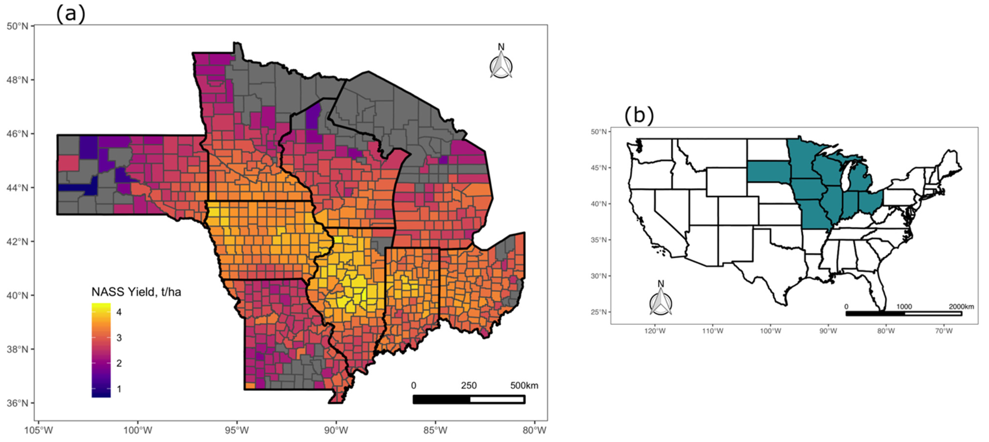
2.1. Study Area
2.2. Yield Data
2.3. Satellite Data
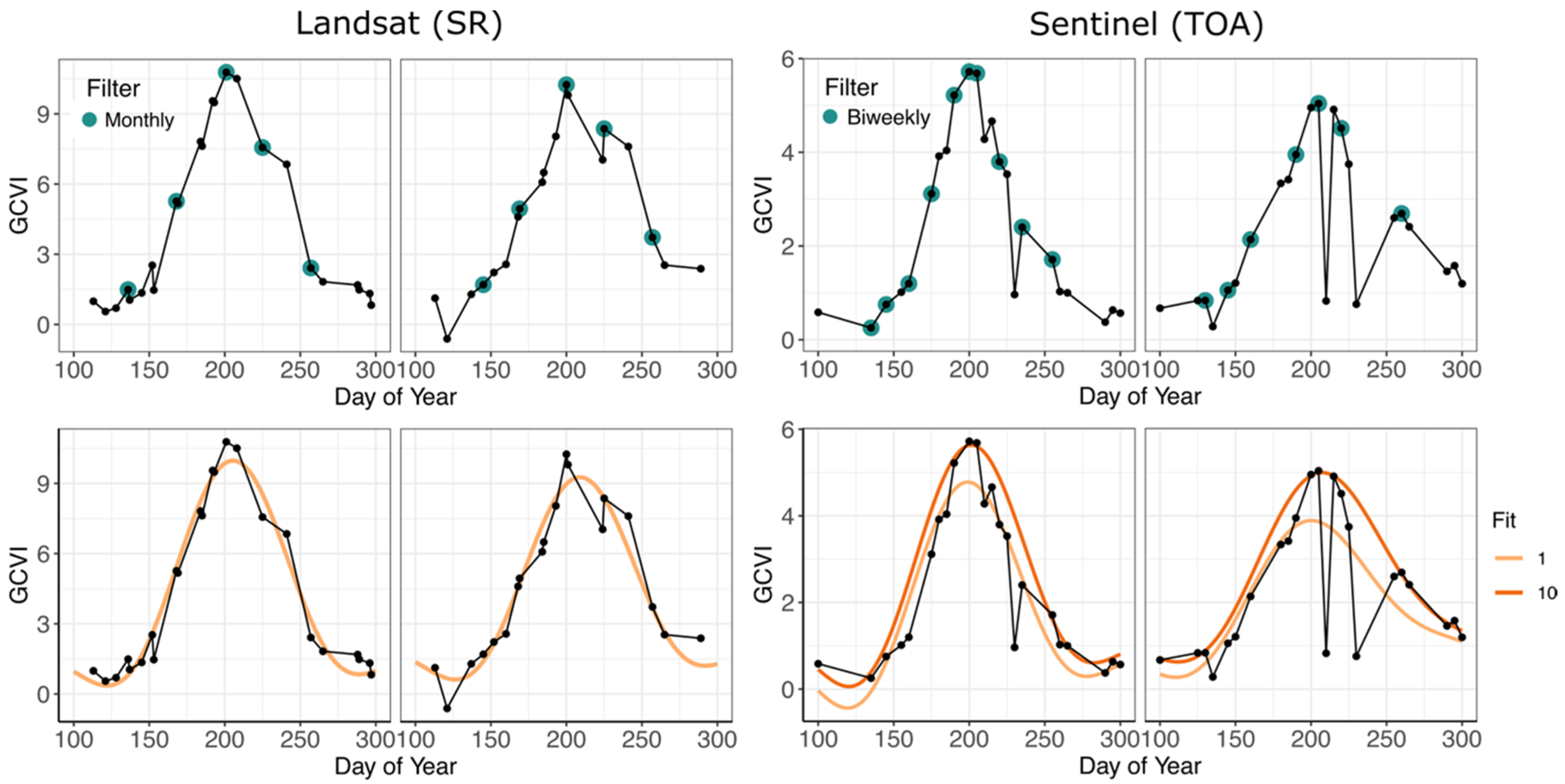
2.4. Harmonic Regressions and Feature Engineering
2.5. Modeling Approach
2.5.1. Training, Validation, and Test Data
2.5.2. Pixel Scale Random Forest Models
2.5.3. County Scale Random Forest Models
2.5.4. Pixel Scale Simulations-Based Model
3. Results
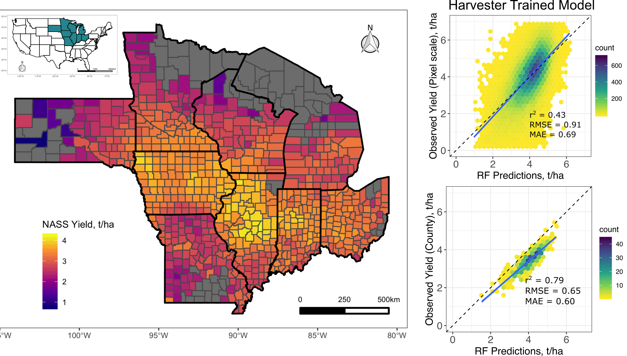
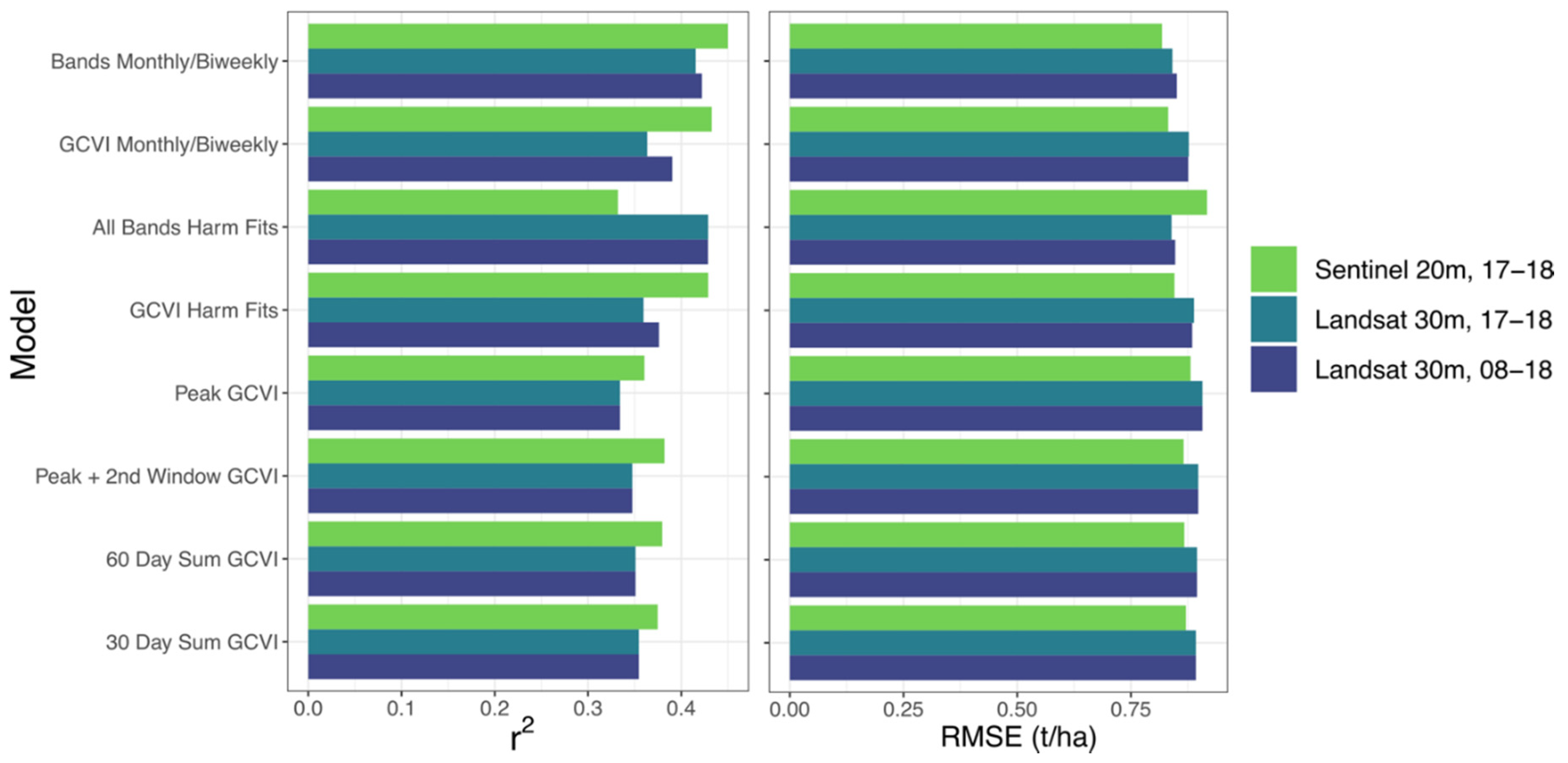
3.1. Pixel Scale Random Forest Models
3.2. County-Scale Random Forest Models
3.3. Simulations-Based Models (SCYM)
4. Discussion
4.1. Pixel-Scale Yield Prediction
4.2. County-Scale Yield Prediction
4.3. Scalable Yield Mapping
5. Conclusions
Supplementary Materials
Author Contributions
Funding
Acknowledgments
Conflicts of Interest
References
- Jain, M.; Singh, B.; Rao, P.; Srivastava, A.K.; Poonia, S.; Blesh, J.; Azzari, G.; McDonald, A.J.; Lobell, D.B. The impact of agricultural interventions can be doubled by using satellite data. Nat. Sustain. 2019, 2, 931–934. [Google Scholar] [CrossRef]
- Lobell, D.B. The use of satellite data for crop yield gap analysis. Field Crop. Res. 2013, 143, 56–64. [Google Scholar] [CrossRef]
- Basso, B.; Dumont, B.; Cammarano, D.; Pezzuolo, A.; Marinello, F.; Sartori, L. Environmental and economic benefits of variable rate nitrogen fertilization in a nitrate vulnerable zone. Sci. Total Environ. 2016, 227–235. [Google Scholar] [CrossRef] [PubMed]
- Diker, K.; Heermann, D.; Brodahl, M. Frequency Analysis of Yield for Delineating Yield Response Zones. Precis. Agric. 2004, 5, 435–444. [Google Scholar] [CrossRef]
- Hunt, M.L.; Blackburn, G.A.; Carrasco, L.; Redhead, J.W.; Rowland, C.S. High resolution wheat yield mapping using Sentinel-2. Remote Sens. Environ. 2019, 233, 111410. [Google Scholar] [CrossRef]
- Kayad, A.; Sozzi, M.; Gatto, S.; Marinello, F.; Pirotti, F. Monitoring Within-Field Variability of Corn Yield using Sentinel-2 and Machine Learning Techniques. Remote Sens. 2019, 11, 2873. [Google Scholar] [CrossRef]
- You, J.; Li, X.; Low, M.; Lobell, D.; Ermon, S. Deep Gaussian process for crop yield prediction based on remote sensing data. In Proceedings of the 31st AAAI Conference on Artificial Intelligence, San Francisco, CA, USA, 4–9 February 2017; pp. 4559–4565. [Google Scholar]
- Gao, F.; Anderson, M.; Daughtry, C.S.T.; Johnson, D. Assessing the Variability of Corn and Soybean Yields in Central Iowa Using High Spatiotemporal Resolution Multi-Satellite Imagery. Remote Sens. 2018, 10, 1489. [Google Scholar] [CrossRef]
- Jin, Z.; Azzari, G.; Lobell, D.B. Improving the accuracy of satellite-based high-resolution yield estimation: A test of multiple scalable approaches. Agric. For. Meteorol. 2017, 247, 207–220. [Google Scholar] [CrossRef]
- Kang, Y.; Ozdogan, M. Field-level crop yield mapping with Landsat using a hierarchical data assimilation approach. Remote Sens. Environ. 2019, 228, 144–163. [Google Scholar] [CrossRef]
- Maestrini, B.; Basso, B. Drivers of within-field spatial and temporal variability of crop yield across the US Midwest. Sci. Rep. 2018, 8, 14833. [Google Scholar] [CrossRef]
- Robertson, M.J.; Llewellyn, R.S.; Mandel, R.; Lawes, R.; Bramley, R.G.V.; Swift, L.; Metz, N.; O’Callaghan, C. Adoption of variable rate fertiliser application in the Australian grains industry: Status, issues and prospects. Precis. Agric. 2011, 13, 181–199. [Google Scholar] [CrossRef]
- Rodriguez-Galiano, V.; Ghimire, B.; Rogan, J.; Chica-Olmo, M.; Rigol-Sanchez, J. An assessment of the effectiveness of a random forest classifier for land-cover classification. ISPRS J. Photogramm. Remote Sens. 2012, 67, 93–104. [Google Scholar] [CrossRef]
- Wang, S.; Azzari, G.; Lobell, D.B. Crop type mapping without field-level labels: Random forest transfer and unsupervised clustering techniques. Remote Sens. Environ. 2019, 222, 303–317. [Google Scholar] [CrossRef]
- Gislason, P.O.; Benediktsson, J.A.; Sveinsson, J.R. Random Forests for land cover classification. Pattern Recognit. Lett. 2006, 27, 294–300. [Google Scholar] [CrossRef]
- Belgiu, M.; Drăguţ, L. Random forest in remote sensing: A review of applications and future directions. ISPRS J. Photogramm. Remote Sens. 2016, 114, 24–31. [Google Scholar] [CrossRef]
- Jin, Z.; Azzari, G.; You, C.; Di Tommaso, S.; Aston, S.; Burke, M.; Lobell, D.B. Smallholder maize area and yield mapping at national scales with Google Earth Engine. Remote Sens. Environ. 2019, 228, 115–128. [Google Scholar] [CrossRef]
- Saeed, U.; Dempewolf, J.; Becker-Reshef, I.; Khan, A.; Ahmad, A.; Wajid, S.A. Forecasting wheat yield from weather data and MODIS NDVI using Random Forests for Punjab province, Pakistan. Int. J. Remote Sens. 2017, 38, 4831–4854. [Google Scholar] [CrossRef]
- Schwalbert, R.A.; Amado, T.; Corassa, G.; Pott, L.P.; Prasad, P.; Ciampitti, I.A. Satellite-based soybean yield forecast: Integrating machine learning and weather data for improving crop yield prediction in southern Brazil. Agric. For. Meteorol. 2020, 284, 107886. [Google Scholar] [CrossRef]
- Breiman, L. Random Forests. Mach. Learn. 2001, 45, 5–32. [Google Scholar] [CrossRef]
- Aghighi, H.; Azadbakht, M.; Ashourloo, D.; Shahrabi, H.S.; Radiom, S. Machine Learning Regression Techniques for the Silage Maize Yield Prediction Using Time-Series Images of Landsat 8 OLI. IEEE J. Sel. Top. Appl. Earth Obs. Remote Sens. 2018, 11, 4563–4577. [Google Scholar] [CrossRef]
- Yue, J.; Feng, H.; Yang, G.; Li, Z. A Comparison of Regression Techniques for Estimation of Above-Ground Winter Wheat Biomass Using Near-Surface Spectroscopy. Remote Sens. 2018, 10, 66. [Google Scholar] [CrossRef]
- Cai, Y.; Guan, K.; Lobell, D.B.; Potgieter, A.B.; Wang, S.; Peng, J.; Xu, T.; Asseng, S.; Zhang, Y.; You, L.; et al. Integrating satellite and climate data to predict wheat yield in Australia using machine learning approaches. Agric. For. Meteorol. 2019, 274, 144–159. [Google Scholar] [CrossRef]
- Richetti, J.; Judge, J.; Boote, K.J.; Johann, J.A.; Opazo, M.A.U.; Becker, W.R.; Paludo, A.; Silva, L.C.D.A. Using phenology-based enhanced vegetation index and machine learning for soybean yield estimation in Paraná State, Brazil. J. Appl. Remote Sens. 2018, 12, 026029. [Google Scholar] [CrossRef]
- Han, L.; Yang, G.; Dai, H.; Xu, B.; Yang, H.; Feng, H.; Li, Z.; Yang, X. Modeling maize above-ground biomass based on machine learning approaches using UAV remote-sensing data. Plant Methods 2019, 15, 1–19. [Google Scholar] [CrossRef] [PubMed]
- Lobell, D.B.; Thau, D.; Seifert, C.; Engle, E.; Little, B. A scalable satellite-based crop yield mapper. Remote Sens. Environ. 2015, 164, 324–333. [Google Scholar] [CrossRef]
- Burke, M.; Lobell, D.B. Satellite-based assessment of yield variation and its determinants in smallholder African systems. Proc. Natl. Acad. Sci. USA 2017, 114, 2189–2194. [Google Scholar] [CrossRef]
- Jain, M.; Srivastava, A.K.; Singh, B.; Joon, R.K.; McDonald, A.; Royal, K.; Lisaius, M.C.; Lobell, D.B. Mapping Smallholder Wheat Yields and Sowing Dates Using Micro-Satellite Data. Remote Sens. 2016, 8, 860. [Google Scholar] [CrossRef]
- Sun, J.; Di, L.; Sun, Z.; Shen, Y.; Lai, Z. County-Level Soybean Yield Prediction Using Deep CNN-LSTM Model. Sensors 2019, 19, 4363. [Google Scholar] [CrossRef] [PubMed]
- Margono, B.A.; Turubanova, S.; Zhuravleva, I.; Potapov, P.; Tyukavina, A.; Baccini, A.; Goetz, S.; Hansen, M.C. Mapping and monitoring deforestation and forest degradation in Sumatra (Indonesia) using Landsat time series data sets from 1990 to 2010. Environ. Res. Lett. 2012, 7, 034010. [Google Scholar] [CrossRef]
- Zhu, Z.; Woodcock, C.E. Continuous change detection and classification of land cover using all available Landsat data. Remote Sens. Environ. 2014, 144, 152–171. [Google Scholar] [CrossRef]
- Drusch, M.; Del Bello, U.; Carlier, S.; Colin, O.; Fernandez, V.; Gascon, F.; Hoersch, B.; Isola, C.; Laberinti, P.; Martimort, P.; et al. Sentinel-2: ESA’s Optical High-Resolution Mission for GMES Operational Services. Remote Sens. Environ. 2012, 120, 25–36. [Google Scholar] [CrossRef]
- Clevers, J.; Gitelson, A. Remote estimation of crop and grass chlorophyll and nitrogen content using red-edge bands on Sentinel-2 and -3. Int. J. Appl. Earth Obs. Geoinf. 2013, 23, 344–351. [Google Scholar] [CrossRef]
- Delegido, J.; Verrelst, J.; Alonso, L.; Moreno, J. Evaluation of Sentinel-2 Red-Edge Bands for Empirical Estimation of Green LAI and Chlorophyll Content. Sensors 2011, 11, 7063–7081. [Google Scholar] [CrossRef]
- Kira, O.; Nguy-Robertson, A.L.; Arkebauer, T.J.; Linker, R.; Gitelson, A.A. Informative spectral bands for remote green LAI estimation in C3 and C4 crops. Agric. For. Meteorol. 2016, 243–249. [Google Scholar] [CrossRef]
- Sun, Y.; Qin, Q.; Ren, H.; Zhang, T.; Chen, S. Red-Edge Band Vegetation Indices for Leaf Area Index Estimation From Sentinel-2/MSI Imagery. IEEE Trans. Geosci. Remote Sens. 2019, 58, 826–840. [Google Scholar] [CrossRef]
- Nguy-Robertson, A.; Gitelson, A.A.; Peng, Y.; Viña, A.; Arkebauer, T.; Rundquist, D. Green Leaf Area Index Estimation in Maize and Soybean: Combining Vegetation Indices to Achieve Maximal Sensitivity. Agron. J. 2012, 104, 1336–1347. [Google Scholar] [CrossRef]
- USDA ERS. Soybeans & Oil Crops. Available online: https://www.ers.usda.gov/topics/crops/soybeans-oil-crops/ (accessed on 14 May 2020).
- USDA ERS. Oil Crops Sector at a Glance. Available online: https://www.ers.usda.gov/topics/crops/soybeans-oil-crops/oil-crops-sector-at-a-glance/ (accessed on 29 March 2020).
- National Agricultural Statistics Service United States Summary and State Data 2012 Census Agric. Available online: https://www.nass.usda.gov/Publications/AgCensus/2012/ (accessed on 2 May 2014).
- NASS. Quick Stats|Ag Data Commons. Available online: https://data.nal.usda.gov/dataset/nass-quick-stats (accessed on 5 September 2020).
- Abatzoglou, J.T. Development of gridded surface meteorological data for ecological applications and modelling. Int. J. Clim. 2011, 33, 121–131. [Google Scholar] [CrossRef]
- Fulton, J.; Hawkins, E.; Taylor, R.; Franzen, A.; Shannon, D.; Clay, D.; Kitchen, N. Yield Monitoring and Mapping. Precis. Agric. Basics 2018, 63–77. [Google Scholar] [CrossRef]
- Gorelick, N.; Hancher, M.; Dixon, M.; Ilyushchenko, S.; Thau, D.; Moore, R. Google Earth Engine: Planetary-scale geospatial analysis for everyone. Remote Sens. Environ. 2017, 202, 18–27. [Google Scholar] [CrossRef]
- Vogelmann, J.E.; Gallant, A.L.; Shi, H.; Zhu, Z. Perspectives on monitoring gradual change across the continuity of Landsat sensors using time-series data. Remote Sens. Environ. 2016, 185, 258–270. [Google Scholar] [CrossRef]
- Gitelson, A.A.; Viña, A.; Arkebauer, T.J.; Rundquist, D.; Keydan, G.; Leavitt, B. Remote estimation of leaf area index and green leaf biomass in maize canopies. Geophys. Res. Lett. 2003, 30. [Google Scholar] [CrossRef]
- Sola, I.; Álvarez-Mozos, J.; González-Audícana, M. Inter-comparison of atmospheric correction methods on Sentinel-2 images applied to croplands. Int. Geosci. Remote Sens. Symp. 2018, 5940–5943. [Google Scholar] [CrossRef]
- Rumora, L.; Miler, M.; Medak, D. Impact of Various Atmospheric Corrections on Sentinel-2 Land Cover Classification Accuracy Using Machine Learning Classifiers. ISPRS Int. J. Geo-Inf. 2020, 9, 277. [Google Scholar] [CrossRef]
- Sola, I.; García-Martín, A.; Sandonís-Pozo, L.; Álvarez-Mozos, J.; Pérez-Cabello, F.; González-Audícana, M.; Llovería, R.M. Assessment of atmospheric correction methods for Sentinel-2 images in Mediterranean landscapes. Int. J. Appl. Earth Obs. Geoinf. 2018, 73, 63–76. [Google Scholar] [CrossRef]
- Friedman, J.H. Recent Advances in Predictive (Machine) Learning. J. Classif. 2006, 23, 175–197. [Google Scholar] [CrossRef]
- Coluzzi, R.; Imbrenda, V.; Lanfredi, M.; Simoniello, T. A first assessment of the Sentinel-2 Level 1-C cloud mask product to support informed surface analyses. Remote Sens. Environ. 2018, 217, 426–443. [Google Scholar] [CrossRef]
- Lobell, D.B.; Di Di Tommaso, S.; You, C.; Djima, I.Y.; Burke, M.; Kilic, T. Sight for Sorghums: Comparisons of Satellite- and Ground-Based Sorghum Yield Estimates in Mali. Remote Sens. 2019, 12, 100. [Google Scholar] [CrossRef]
- Waldner, F.; Horan, H.; Chen, Y.; Hochman, Z. High temporal resolution of leaf area data improves empirical estimation of grain yield. Sci. Rep. 2019, 9, 1–14. [Google Scholar] [CrossRef]
- Varoquaux, G.; Buitinck, L.; Louppe, G.; Grisel, O.; Pedregosa, F.; Mueller, A. Scikit-learn. GetMobile: Mob. Comput. Commun. 2015, 19, 29–33. [Google Scholar] [CrossRef]
- Jordan, C.F. Derivation of Leaf-Area Index from Quality of Light on the Forest Floor. Ecology 1969, 50, 663–666. [Google Scholar] [CrossRef]
- Gitelson, A.A.; Kaufman, Y.J.; Merzlyak, M.N. Use of a green channel in remote sensing of global vegetation from EOS-MODIS. Remote Sens. Environ. 1996, 58, 289–298. [Google Scholar] [CrossRef]
- Badgley, G.; Field, C.B.; Berry, J.A. Canopy near-infrared reflectance and terrestrial photosynthesis. Sci. Adv. 2017, 3, 1602244. [Google Scholar] [CrossRef]
- Rondeaux, G.; Steven, M.; Baret, F. Optimization of soil-adjusted vegetation indices. Remote Sens. Environ. 1996, 55, 95–107. [Google Scholar] [CrossRef]
- Pasqualotto, N.; Delegido, J.; Van Wittenberghe, S.; Rinaldi, M.; Moreno, J. Multi-Crop Green LAI Estimation with a New Simple Sentinel-2 LAI Index (SeLI). Sensors 2019, 19, 904. [Google Scholar] [CrossRef] [PubMed]
- Dash, J.; Curran, P.J. The MERIS terrestrial chlorophyll index. Int. J. Remote Sens. 2004, 25, 5403–5413. [Google Scholar] [CrossRef]
- Daughtry, C. Estimating Corn Leaf Chlorophyll Concentration from Leaf and Canopy Reflectance. Remote Sens. Environ. 2000, 74, 229–239. [Google Scholar] [CrossRef]
- Gitelson, A.; Merzlyak, M.N. Quantitative estimation of chlorophyll-a using reflectance spectra: Experiments with autumn chestnut and maple leaves. J. Photochem. Photobiol. B Biol. 1994, 22, 247–252. [Google Scholar] [CrossRef]
- Rouse, J.W.; Haas, R.H.; Schell, J.A.; Deering, D.W. Monitoring veg- etation systems in the Great Plains with ERTS. In Proceedings of the Third Earth Resources Technology Satellite Symposium, Washington, DC, USA, 10–14 December 1974; pp. 309–317. [Google Scholar]
- Boryan, C.; Yang, Z.; Mueller, R.; Craig, M. Monitoring US agriculture: The US Department of Agriculture, National Agricultural Statistics Service, Cropland Data Layer Program. Geocarto Int. 2011, 26, 341–358. [Google Scholar] [CrossRef]
- Holzworth, D.P.; Huth, N.I.; Devoil, P.G.; Zurcher, E.J.; Herrmann, N.I.; McLean, G.; Chenu, K.; Van Oosterom, E.J.; Snow, V.; Murphy, C.; et al. APSIM—Evolution towards a new generation of agricultural systems simulation. Environ. Model. Softw. 2014, 62, 327–350. [Google Scholar] [CrossRef]
- Lobell, D.B.; Azzari, G. Satellite detection of rising maize yield heterogeneity in the U.S. Midwest. Environ. Res. Lett. 2017, 12, 014014. [Google Scholar] [CrossRef]
- Jin, Z.; Ainsworth, E.A.; Leakey, A.D.B.; Lobell, D.B. Increasing drought and diminishing benefits of elevated carbon dioxide for soybean yields across the US Midwest. Glob. Chang. Biol. 2017, 24, 522–e533. [Google Scholar] [CrossRef] [PubMed]
- Srinivasan, V.; Kumar, P.; Long, S.P. Decreasing, not increasing, leaf area will raise crop yields under global atmospheric change. Glob. Chang. Biol. 2016, 23, 1626–1635. [Google Scholar] [CrossRef] [PubMed]
- Mourtzinis, S.; Specht, J.E.; Lindsey, L.E.; Wiebold, W.J.; Ross, J.; Nafziger, E.D.; Kandel, H.J.; Mueller, N.; DeVillez, P.L.; Arriaga, F.J.; et al. Climate-induced reduction in US-wide soybean yields underpinned by region- and in-season-specific responses. Nat. Plants 2015, 1, 14026. [Google Scholar] [CrossRef] [PubMed]
- Tannura, M.A.; Irwin, S.H.; Good, D.L. Weather, Technology, and Corn and Soybean Yields in the U.S. Corn Belt. SSRN Electron. J. 2008. [Google Scholar] [CrossRef]
- Maimaitijiang, M.; Sagan, V.; Sidike, P.; Hartling, S.; Esposito, F.; Fritschi, F.B. Soybean yield prediction from UAV using multimodal data fusion and deep learning. Remote Sens. Environ. 2020, 237, 111599. [Google Scholar] [CrossRef]
- Guyot, G.; Baret, F.; Jacquemoud, S. Imaging spectroscopy for vegetation studies. Imaging Spectrosc. 1992, 145–165. [Google Scholar]
- Peng, Y.; Nguy-Robertson, A.; Linker, R.; Gitelson, A.A. Assessment of Canopy Chlorophyll Content Retrieval in Maize and Soybean: Implications of Hysteresis on the Development of Generic Algorithms. Remote Sens. 2017, 9, 226. [Google Scholar] [CrossRef]
- Whitcraft, A.K.; Vermote, E.F.; Becker-Reshef, I.; Justice, C. Cloud cover throughout the agricultural growing season: Impacts on passive optical earth observations. Remote Sens. Environ. 2015, 156, 438–447. [Google Scholar] [CrossRef]
- Lobell, D.B.; Azzari, G.; Burke, M.; Gourlay, S.; Jin, Z.; Kilic, T.; Murray, S. Eyes in the Sky, Boots on the Ground: Assessing Satellite- and Ground-Based Approaches to Crop Yield Measurement and Analysis. Am. J. Agric. Econ. 2019, 102, 202–219. [Google Scholar] [CrossRef]


| Model | Satellite Data | Training Response Variable | Testing Response Variable | Machine Learning Algorithm | Research Question |
|---|---|---|---|---|---|
| Landsat harvester trained | 30 m Landsat | 30 m harvester yields | 30 m harvester yields AND county yields | Random Forest | How well can a machine learning model, trained using pixel-scale harvester yields, perform both at the pixel- and county-scale? |
| Sentinel-2 harvester trained | 20 m Sentinel-2 | 20 m harvester yields | 20 m harvester yields | Random Forest | Does the additional spectral precision of Sentinel-2 help compared to the same years/test sites using Landsat? Do red-edge vegetation indices add signal? |
| County-trained model | Landsat, sampled and aggregated to county scale | County Yields | County yields AND 30 m harvester yields | Random Forest | How does a model trained with aggregated, freely available data compare to a model trained with pixel-scale data in performance at both pixel and county scales? |
| Simulations-based SCYM Model | 30 m Landsat | Simulated crop yields | 30 m harvester yields AND county yields | Multiple Linear Regression | How does a model trained with simulated data perform on pixel-scale test data? Do insights from the 30 m harvest-trained model improve SCYM methodology? |
| Year | Point Sample Distribution | Points after Landsat Filter | Points after Sentinel Filter |
|---|---|---|---|
| 2008 | 32,343 | 15,745 | |
| 2009 | 28,385 | 13,653 | |
| 2010 | 37,163 | 17,946 | |
| 2011 | 29,761 | 18,086 | |
| 2012 | 35,772 | 1792 | |
| 2013 | 34,884 | 16,057 | |
| 2014 | 37,823 | 18,442 | |
| 2015 | 32,940 | 15,766 | |
| 2016 | 39,029 | 25,134 | |
| 2017 | 38,647 | 24,412 | 15,436 |
| 2018 | 35,108 | 19,127 | 24,142 |
| Vegetation Index | Citation | Equation |
|---|---|---|
| Simple Ratio (SR) | Jordan, 1969 [55] | |
| Normalized Difference Vegetation Index (NDVI) | Rouse et al., 1973 [63] | |
| Green Chlorophyl Vegetation Index (GCVI) | Gitelson et al., 1996 [56] | |
| Near Infrared Reflectance of vegetation (NIRv) | Badgley et al., 2017 [57] | |
| Optimized Soil Adjusted Vegetation Index (OSAVI) | Rondeaux et al., 1996 [58] | |
| Sentinel-2 LAI-Green Index (SeLI) | Pasqualotto et al., 2019 [59] | |
| MERIS Terrestrial Chlorphyl Index (MTCI) | Dash and Curran, 2004 [60] | |
| Modified Chlorohyl Absorption in Reflectance Index (MCARI) | Daughtry et al., 2000 [61] | |
| Chlorophyl Index, Red-Edge (Cir) | Gitelson et al., 2003 [46] | |
| Normalized Difference Red Edge Index, 1 (NDRE1) | Gitelson and Merzlyak, 1994 [62] | |
| Normalized Difference Red Edge Index, 2 (NDRE2) | Gitelson and Merzlyak, 1994 [62] |
| Factor | Values Used | Units | Comments |
|---|---|---|---|
| Year | 2007–13 | ||
| Site | Newton, IA (−93.1°E, 41.7°N) Marshalltown, IA (−92.9°E, 42.1°N) Clinton, IL (−89.0°E, 40.1°N) Chenoa, IL (−88.7°E, 40.7°N) Marion, IN (−85.7°E, 40.6°N) Munice, IN (−85.3°E, 40.2°N) Benson, MN (−95.6°E, 45.3°N) Aberdeen, SD (−98.5°E, 45.5°N) | Latter two sites added from baseline | |
| Fertilizer Rate | 0, 25, 50 | kg of urea N per ha | |
| Sowing Density | 3, 5, 7 | Plants per m2 | |
| Row Spacing | 380 | mm | Reduced from baseline as per [67] |
| Cultivar Choice | Pioneer93M42 3.4, Pioneer_94B01 4.0 | Similar cultivars as [67] | |
| Soil Water At Sowing | 0.8, 1.0 | % of total water holding capacity | |
| Sow Date | April 25, May 5, May 20, June 14 | Added April 25th date for additional variability |
| Vegetation Index | r2 | RMSE (t/ha) | MAE (t/ha) |
|---|---|---|---|
| SR | 0.42 | 0.841 | 0.648 |
| NDVI | 0.42 | 0.840 | 0.648 |
| GCVI | 0.43 | 0.832 | 0.641 |
| NIRv | 0.45 | 0.822 | 0.634 |
| OSAVI | 0.42 | 0.839 | 0.648 |
| SeLI | 0.44 | 0.828 | 0.638 |
| MTCI | 0.39 | 0.863 | 0.665 |
| MCARI | 0.29 | 0.932 | 0.720 |
| Cir | 0.44 | 0.829 | 0.638 |
| NDRE1 | 0.43 | 0.835 | 0.643 |
| NDRE2 | 0.44 | 0.829 | 0.637 |
| SCYM Model | r2 | RMSE (t/ha) | MAE (t/ha) |
|---|---|---|---|
| Baseline 2-Window | 0.24 | 1.09 | 0.86 |
| Peak GCVI, Met | 0.25 | 1.00 | 0.77 |
| Peak GCVI, Aug Rain | 0.26 | 0.96 | 0.74 |
| Peak GCVI, No Met | 0.24 | 0.98 | 0.75 |
| Peak GCVI, DOY, Met | 0.18 | 1.11 | 0.85 |
| 60d Sum, No Met | 0.23 | 1.42 | 1.15 |
| 60d Sum | 0.24 | 1.05 | 0.83 |
| 60d Sum, Aug Rain | 0.24 | 1.12 | 0.90 |
| 30d Sum, No Met | 0.24 | 1.00 | 0.80 |
| 30d Sum, Met | 0.25 | 0.98 | 0.75 |
| 30d Sum, Aug Rain | 0.24 | 1.00 | 0.76 |
| Peak + 2nd Window, No Met | 0.26 | 0.97 | 0.76 |
| Peak + 2nd Window, Met | 0.27 | 1.01 | 0.79 |
| Peak + 2nd Window, Aug Rain | 0.27 | 0.96 | 0.75 |
Publisher’s Note: MDPI stays neutral with regard to jurisdictional claims in published maps and institutional affiliations. |
© 2020 by the authors. Licensee MDPI, Basel, Switzerland. This article is an open access article distributed under the terms and conditions of the Creative Commons Attribution (CC BY) license (http://creativecommons.org/licenses/by/4.0/).
Share and Cite
Dado, W.T.; Deines, J.M.; Patel, R.; Liang, S.-Z.; Lobell, D.B. High-Resolution Soybean Yield Mapping Across the US Midwest Using Subfield Harvester Data. Remote Sens. 2020, 12, 3471. https://doi.org/10.3390/rs12213471
Dado WT, Deines JM, Patel R, Liang S-Z, Lobell DB. High-Resolution Soybean Yield Mapping Across the US Midwest Using Subfield Harvester Data. Remote Sensing. 2020; 12(21):3471. https://doi.org/10.3390/rs12213471
Chicago/Turabian StyleDado, Walter T., Jillian M. Deines, Rinkal Patel, Sang-Zi Liang, and David B. Lobell. 2020. "High-Resolution Soybean Yield Mapping Across the US Midwest Using Subfield Harvester Data" Remote Sensing 12, no. 21: 3471. https://doi.org/10.3390/rs12213471
APA StyleDado, W. T., Deines, J. M., Patel, R., Liang, S.-Z., & Lobell, D. B. (2020). High-Resolution Soybean Yield Mapping Across the US Midwest Using Subfield Harvester Data. Remote Sensing, 12(21), 3471. https://doi.org/10.3390/rs12213471