Recent Climate Change Feedbacks to Greenland Ice Sheet Mass Changes from GRACE

Abstract

Although a significant effort has been dedicated to studying changes in the mass budget of the Greenland Ice Sheet (GrIS), mechanisms behind these changes are not yet fully understood. In this study, we address this issue by investigating the link between climate controls and mass changes of the GrIS between August 2002 and June 2017. We estimate the GrIS mass changes based on averaging the Gravity Recovery and Climate Experiment (GRACE) monthly gravity field solutions from four processing data centers. We then investigate the possible impact of different climate variables on the GrIS mass changes using the North Atlantic Oscillation (NAO), temperature, precipitation, and the 700 hPa wind retrieved from the ERA-5 reanalysis. Results indicate a decrease of −267.77 ± 32.67 Gt/yr in the total mass of the GrIS over the 16-year period. By quantifying the relationship between climate controls and mass changes, we observe that mass changes in different parts of Greenland have varying sensitivity to climate controls. The NAO mainly controls mass changes in west Greenland, where the summertime NAO modulations have a greater impact on the summer mass loss than the wintertime NAO modulations have on the winter mass gain. The GrIS mass changes are correlated spatially with summer temperature, especially in southwest Greenland. Mass balance changes in northwest Greenland are mostly affected by wind anomalies. These new findings based on wind anomalies indicate that the summer atmospheric circulation anomalies control surface temperature and snow precipitation and consequently affect mass changes in different parts of Greenland.

1. Introduction

The Greenland Ice Sheet (GrIS) (Figure 1) has been losing mass at a rate that is a major contribution to global sea-level rise in recent decades [1,2,3,4,5,6]. Mechanisms behind the mass changes of the GrIS are not yet fully understood, particularly the impact of climate change on different areas of Greenland. Monitoring the GrIS mass balance is essential for understanding global sea level change, the global water cycle, and other issues associated with climate change [7,8]. Satellite remote-sensing techniques have primarily been used to detect changes in the GrIS, such as the Global Navigation Satellite Systems technique [1,9,10], satellite altimetry [11,12,13,14,15], and satellite gravity [16,17,18,19]. The Gravity Recovery and Climate Experiment (GRACE) space mission in the terrestrial gravity field from space has been successfully used to monitor the mass changes in Greenland from temporal variations in space [20,21,22,23].

The mass changes of the GrIS detected by GRACE are the sum of mass variations in the glacial dynamic mass balance (ice discharge) and the surface mass balance (SMB) [8,24,25,26,27], but GRACE observations cannot directly separate these physical causes. Previous studies used the SMB and ice discharge data for a detailed analysis and validation of GRACE results [12,23]. Mouginot et al. (2019) [28] provided a detailed and comprehensive review of spatial and temporal mass changes of Greenland’s glaciers using regional atmospheric climate model and glacier ice discharge data from velocity-scaled reference fluxes between 1972 and 2018. Zou et al. (2020) [29] analyzed the temporal and spatial distribution of mass changes in Greenland over the past 15 years by using GRACE, SMB, and ice discharge data. The main purpose of this study is to investigate mechanisms behind mass changes when we used the GRACE mass change results in our analysis without separating the individual signals.

The GrIS mass changes are affected by climate variability, especially related to the near-surface air temperature [25,30,31], precipitation [32,33], and atmospheric circulation [34,35]. In this study, we attempt to better understand possible mechanisms that control inconsistent mass changes throughout Greenland. Fettweis et al. (2013) [36] found that negative phases of the North Atlantic Oscillation (NAO) index occurred more frequently in the summer, leading to an increased northward transport of warm air to Greenland. Bevis et al. (2019) [1] reported on the relationship of mass changes of the GrIS with NAO and atmospheric forcing, like air temperature and solar radiation. They found that the sustained acceleration and the abrupt deceleration of mass loss were mostly driven by changes in air temperature and solar radiation. Hanna et al. (2014) [37] analyzed the summer 500 hPa geopotential height field in the northern hemisphere. They pointed out that the blocking of high pressure over Greenland has a high correlation coefficient with surface melting. Tedesco et al. (2008) [32] pointed out that the warming and persistent surface temperature anomalies of the GrIS are directly related to a surface ice melting in Greenland. Seo et al. (2015) [32] reported that decreased precipitation significantly contributed to the ice mass loss acceleration before 2010. Bezeau et al. (2015) [35] demonstrated that a statistically significant increase in the frequency of anticyclonic circulations over Greenland resulted in more negative glacier mass balance between 2007 and 2012.

Although the connection between the GrIS mass changes and climate controls has generally been recognized, detailed studies of their impact for specific parts of Greenland have not yet been done. Moreover, these studies involved only temperature and precipitation, while a possible impact of wind anomalies on the GrIS mass changes as well as a possible interconnection between these climate controls are not yet fully understood. In this study, we quantified typical and abnormal impacts of large-scale atmospheric circulation (e.g., NAO) and regional climate controls (temperature, precipitation, and wind anomalies) on mass changes for different parts of Greenland. By quantifying the relationships between these investigated phenomena, we were able to understand better the impact mechanisms and magnitude of each climate factor with respect to the GrIS mass changes.

Our study is organized as follows. First, we investigated and compared estimates of the GrIS mass balance changes obtained from the GRACE time-varying gravity field between 2002 and 2017. We then provided a detailed analysis of interannual changes and long-term trends, followed by examining possible explanations of these mass changes, using NAO indices, precipitation, surface temperature, and wind profile in Greenland and its adjacent seas, which was provided by the European Centre for Medium Term Weather Forecasting (ECMWF). Finally, we investigated the characteristics of each climate factor that influences the GrIS mass changes and the associated mechanisms behind their influence on the summer mass changes for selected years. The article is organized into four sections, with data acquisition in Section 2 and methods described in Section 3. The results are presented and analyzed in Section 4, with the major findings summarized in Section 5.

2. Data

Input data and models used for estimating the mass balance changes of the GrIS and their further classification in terms of various climate variables are briefly described in this section.

2.1. GRACE Data

GRACE was launched on March 2002 and provided monthly solutions from April 2002 until June 2017. Many parameter choices and solution strategies have been implemented to derive the relative ranging observations between the two GRACE spacecrafts in order to estimate the month-to-month gravity field variations leading to each center developing different approaches and models used by each center yielding differences in the Level-2 products. A recent study indicated that a simple average of GRACE solutions from different centers was the most effective method to reduce the noise in the gravity field solutions within the available scatter of the solutions [38]. In this study, we adopted this procedure and employed the Level 2 monthly spherical harmonic coefficients from four data center’s solutions, the Geoforschungs Zentrum Potsdam (GFZ), the Center for Space Research (CSR) at the University of Texas in Austin, the Jet Propulsion Laboratory (JPL), and the Institute of Geodesy in Graz (ITSG) with the spherical harmonic degree of 60 from April 2002 to June 2017. To reduce the noise in the gravity field solutions, we adopted mean estimates of the GrIS mass changes based on averaging values from the CSR-RL06, GFZ-RL06, JPL-RL06, and ITSG-2018 models.

The terrestrial water storage anomalies can be computed from these coefficients for a particular time period t according to the following expression in terms of an equivalent water thickness [39]:

$$∆\mathsf{\sigma }\left(\mathsf{\theta },\mathsf{\lambda }\right)=\frac{R\rho }{3{\rho }_w}{{\displaystyle \sum }}_{n=0}^{\tilde{n}}{{\displaystyle \sum }}_{m=0}^n{W}_n{\tilde{P}}_{nm}\left(cos\theta \right)\frac{2n+1}{1+k_n}\left(∆C_{nm}\cos \left(m\lambda \right)+∆S_{nm}\sin \left(m\lambda \right)\right)$$

(1)

where $∆\mathsf{\sigma }\left(\mathsf{\theta },\mathsf{\lambda }\right)$ is the mass change at a point $\left(\mathsf{\theta },\mathsf{\lambda }\right)$, θ and λ are the colatitude and longitude, $\rho$ is the Earth’s mean density, ${\rho }_w$ is the freshwater density, $R$ is the Earth’s equatorial radius, ${\tilde{P}}_{nm}$ are the (fully-normalized) Legendre associated functions of degree n and order m, k_n are the degree-dependent Love numbers, and $W_n$ denote the degree-dependent kernel functions of the Gaussian filter.

The missing monthly data are supplemented by interpolating over this period from the two adjacent months. The first-degree spherical harmonic coefficients that cannot directly be detected by GRACE were determined by combining the GRACE data with numerical ocean models [40]. The spherical harmonics of the degree 2 terms were replaced based on the analysis of the Satellite Laser Ranging measurements [41]. After removing the mean gravity field based on the period from January 2003 to December 2016, the residual spherical harmonic coefficients were obtained to estimate the terrestrial water storage changes (TWS). We applied a 500 km Gaussian filter and the P4M6 destriping filter to reduce systematic and correlated errors [42]. To reduce the ocean–land leakage effect, we applied a forward modeling technique of the GRACE monthly water storages changes results [17]. This procedure comprises the following steps: (1) we converted the GRACE spherical harmonics to the gridded mass anomalies (i.e., the GRACE-derived global mass changes) using spatial filters including the P4M6 and 500 km Gaussian filters as mentioned above. (2) Then, we assigned ocean areas with a uniform layer of water, negatively equaling to the total mass rate over land to make the total ocean mass changes equal to that on land. This procedure yields a new simulated global gridded mass change solution. (3) We converted the simulated gridded mass changes to the normalized spherical harmonic coefficients and truncated them at the degree and order of 60. We applied spatial filters (P4M6 and 500 km Gaussian filters) to these spherical harmonic coefficients in the same way as used in the processing of the GRACE spherical harmonic coefficients in order to obtain the new modeled gridded mass anomalies. (4) Subsequently, we compared the new modeled gridded mass change solution with the GRACE-derived gridded mass change solution. Our goal was to minimize differences between these two solutions by applying iterative approach. For this purpose, we added differences between the GRACE-derived mass anomalies and the modeled mass changes to the modeled mass variations as the reconstructed ‘true’ mass variations at each grid point with a number of iterations. (5) The new reconstructed ‘true’ mass variations were regarded as the updated input values in the step 2. The iteration process (in steps 2 to 5) was terminated after the differences between these two solutions were below a defined threshold. The reconstructed ‘true’ global mass variations solution, which after going through similar spatial filtering and truncation as used in GRACE data processing, provide the modeled global mass variations solution that closely resembles the GRACE-derived global mass changes solution.

By taking into account the annual and semiannual signals, we used an ordinary least-squares fit at each grid point of the reconstructed ‘true’ mass variations in order to estimate the long-term change rate and seasonal changes. Uncertainties in GRACE results are due to errors in the processing of the GRACE data, including spatial filters, Glacial Isostatic Adjustment (GIA) models, handling leakage effects, and how to compute regional mass trends and time-series and estimate uncertainties. The 20% GIA correction was chosen as the uncertainty of the GIA model. This choice is based on the analysis of Paulson et al. (2007). They presumed a rather heuristic ±20% uncertainty in GIA models [43,44]. Moreover, 8% of the estimated mass change was chosen as the uncertainty of the forward modeling technique to reduce the leakage effect according to results of a simulation analysis by Jin et al. (2015) [17]. We selected the uncertainty of the uncorrected GRACE trend to be the 2-sigma value obtained from the regression analysis of the trend estimate (at a 95% confidence interval). Therefore, we regarded the total uncertainties of the GRACE mass changes as the sum of uncertainties in GIA models (20% of GIA correction), the forward modeling technique (8% of the estimated mass changes), and the former error estimates derived from the least-squares fit. All error values in this study follow this description.

2.2. GIA Model

Large GIA uplift rates of 12 mm/yr have been identified by the Global Positioning System network in Greenland [45]. The mass changes associated with the glacial isostatic adjustment have to be taken into consideration in order to estimate mass balance trends from GRACE [46,47]. The two main constituents in any GIA model are the ice (deglaciation) history and the viscosity profile in the mantle. In this study, we used the GIA model (shown in Figure 2 in terms of an equivalent water thickness) prepared by Geruo et al. (2013) to correct the GRACE estimates. This model was compiled based on the ICE-5G deglaciation history, the VM2 viscosity profile, and the PREM-based elastic structure [48]. It assumes a compressible Earth and includes polar wander feedback, degree-one terms, and a self-consistent ocean. The GIA corrections add some uncertainty for mass trends over the GRACE period; a canonical uncertainty range of 20% is often assumed for GIA models [43]. This value is a rule of thumb and comes from looking at results for various viscosity values and alternative deglaciation models for Antarctica and Greenland [43]. This value was adopted when applying uncertainties to the GIA correction for GRACE measurements [44,49,50].

2.3. Climate Data

In this study, we used the monthly tabulated NAO index from NOAA standardized to the period 1981–2010 to investigate the relationship between atmospheric circulation and mass changes [51]. The ERA5 is the fifth generation of the ECMWF reanalysis for global climate and weather [52]. The ERA5 provides hourly estimates of a large number of atmospheric, land, and oceanic climate variables. Currently, these datasets are available from 1979. The monthly mean data variables analyzed in this study include the 700 hPa wind field (U700, V700), the near-surface temperature, and the total precipitation provided with a 0.25° × 0.25° spatial resolution.

3. Methodology

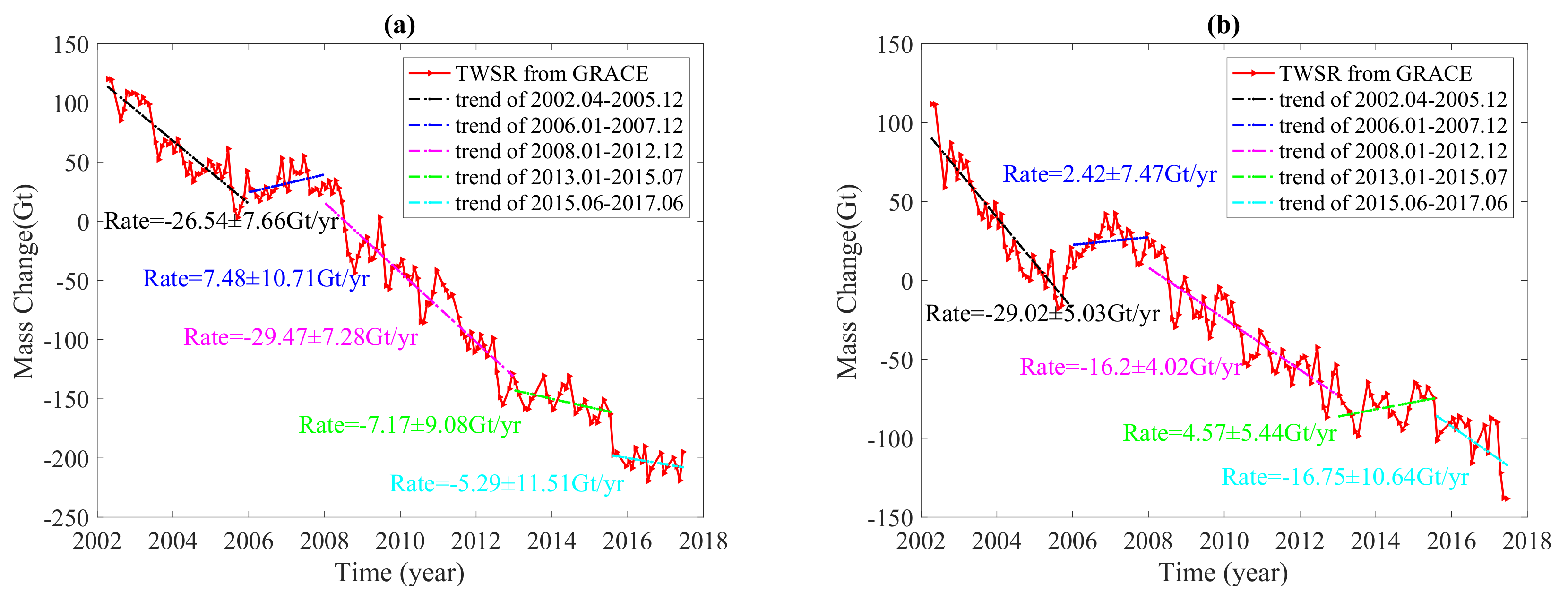
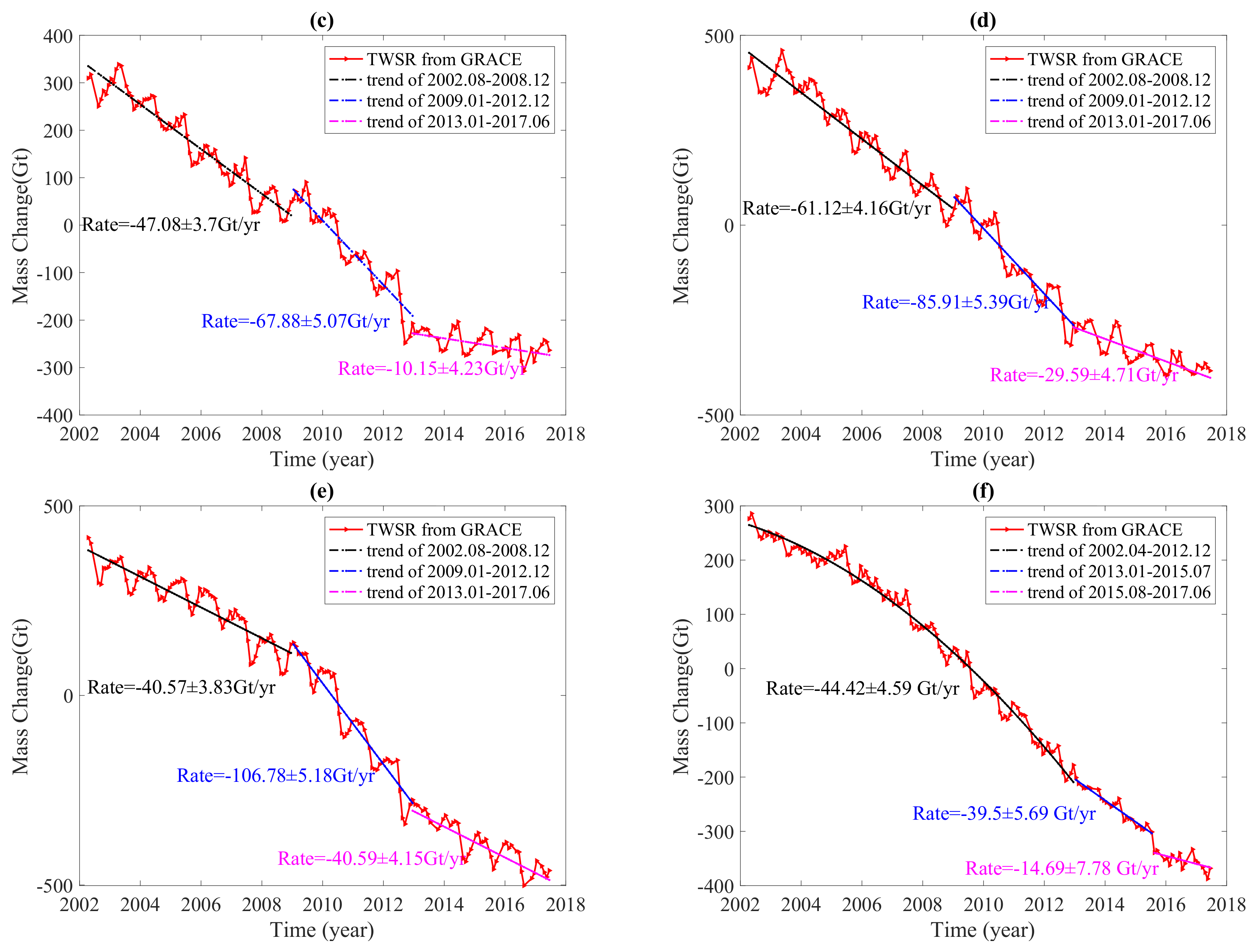
3.1. Time Series Analysis of Mass Changes from GRACE

The long-term trend, the annual and semi-annual components, and the 161-day cyclical fluctuations due to the $S_2$ tide of mass changes from GRACE were estimated using a polynomial regression analysis as follows:

$$\begin{gathered} \mathrm{y}\left(\mathrm{t}\right)=\mathsf{\epsilon }+\mathrm{v}\times t+{\displaystyle \sum }_{i=0}^3{\mathrm{A}}_i\sin \left(\frac{2\pi }{T_i}\left(t-t_0\right)+{\phi }_i\right), \\ {T}_i=1 yr,0.5yr and\frac{161}{365.2}yr \end{gathered}$$

(2)

where y denotes the mass change from GRACE estimates,$t$ is time, $t_0$ is an initial epoch (in this study January 2002), $v$ is the long-term rate of mass changes, $T_i$ represent periods of the cycles considered, $A_i$ is the amplitude of periodic changes, which include the annual and semiannual components as well as 161-day cyclical fluctuations; and ε is the random error. When considering the acceleration of changes of the GrIS, the acceleration term $a\times t^2$ must be added back in Equation (2). Hence

$$\begin{gathered} \mathrm{y}\left(\mathrm{t}\right)=\mathsf{\epsilon }+\mathrm{v}\times t+{\displaystyle \sum }_{i=0}^3{\mathrm{A}}_i\sin \left(\frac{2\pi }{T_i}\left(t-t_0\right)+{\phi }_i\right) +a\times t^2 \\ {T}_i=1 yr,0.5yr and\frac{161}{365.2}yr \end{gathered}$$

(3)

where a is the acceleration rate of mass change.

3.2. Spearman Rank Correlation Coefficient

To determine the relationship between mass changes and climate controls, we applied the Kolmogorov–Smirnov’s method [53] to determine the type of data distribution. We found that these climate control data do not have a normal distribution. We therefore used the Spearman’s rho method [54] to find the correlation between variables.

The Spearman’s correlation coefficient is defined as the Pearson’s correlation coefficient between the rank variables. It reads

$$\rho =1-\frac{6\sum d_i{}^2}{n\left(n^2-1\right)}$$

(4)

where $\rho$ is the Spearman’s rank correlation, $n$ is the number of observations, and $d_i$ is the difference between ranks of the corresponding variables. The correlations in this paper were computed at the 95% confidence level (i.e., p < 0.05).

3.3. Cross-Correlation and Time Lag

We analyzed the cross-correlation between interannual mass changes and climate controls. To verify the correlation results, we also calculated the coherence spectrum. This provides a frequency-dependent measure of correlation magnitude and possibly additional information in the form of phase versus frequency relations.

The cross-correlation $\rho \left(\tau \right)$ measures the similarity between two-time series, $x_1\left(t\right)$ and a shifted (lagged) $x_2\left(t\right)$ as a function of the lag $\tau$ [55], i.e.,

$$\rho \left(\tau \right)=\frac{{\sigma }_{12}\left(\tau \right)}{{\sigma }_{11}{\sigma }_{22}} ,$$

(5)

where ${\sigma }_{12}\left(\tau \right)$ is the cross-covariance function of lag $\tau$ with $x_2\left(t\right)$ leading $x_1\left(t\right)$ and ${\sigma }_{11}$ and are the auto-variances of $x_1\left(t\right)$ and $x_2\left(t\right)$, respectively. The value of $\rho \left(\tau \right)$ lies between ±1.

3.4. Ridge Regression

The presence of serious multicollinearity often affects the usefulness of a fitted model for making predictions [56]. The ridge regression is one effective method that has been proposed to remedy the multicollinearity problem by modifying the method of least squares to allow biased estimators of the regression coefficient [57].

The normal linear regression model reads

$$Y_j={\beta }_0+{\beta }_1{X}_{1j}+{\beta }_2{\beta }_1{X}_{2j}+\cdots +{\beta }_m{X}_{mj}+{\epsilon }_j$$

(6)

where

$$\begin{gathered} \mathrm{X}={\left[\begin{array}{ccccc}1 & {\mathrm{X}}_{11} & {\mathrm{X}}_{21} & \cdots & {\mathrm{X}}_{\mathrm{m}1}\\ 1 & {\mathrm{X}}_{21} & {\mathrm{X}}_{22} & \cdots & {\mathrm{X}}_{\mathrm{m}2}\\ & & \ddots \\ 1 & {\mathrm{X}}_{1\mathrm{n}} & {\mathrm{X}}_{2\mathrm{n}} & \cdots & {\mathrm{X}}_{\mathrm{mn}}\end{array}\right]}_{\mathrm{n}\times \left(\mathrm{m}+1\right)} \\ \mathsf{\beta }={\left[\begin{array}{c}{\mathsf{\beta }}_0\\ {\mathsf{\beta }}_1\\ \begin{array}{c}⋮\\ {\mathsf{\beta }}_{\mathrm{m}}\end{array}\end{array}\right]}_{\left(\mathrm{m}+1\right)\times 1} \\ \mathrm{Y}={\left[\begin{array}{c}{\mathrm{Y}}_1\\ {\mathrm{Y}}_2\\ \begin{array}{c}⋮\\ {\mathrm{Y}}_{\mathrm{n}}\end{array}\end{array}\right]}_{\left(\mathrm{n}+1\right)\times 1} \end{gathered}$$

(7)

For the ordinary least-squares analysis, the system of normal equations is given by

$$\left(\mathrm{X}{}^{\prime }\mathrm{X}\right){\displaystyle \hat{\mathsf{\beta }}}=\mathrm{X}{}^{\prime }\mathrm{Y}$$

(8)

where the least-squares estimate of the regression coefficient β in this model reads

$${\displaystyle \hat{\mathsf{\beta }}}={\left(\mathrm{X}{}^{\prime }\mathrm{X}\right)}^{-1}\mathrm{X}{}^{\prime }\mathrm{Y}$$

(9)

The ridge regression analysis usually needs to first centralize and quantize the X variable, so that different independent variables are of the same order of magnitude for a simple comparison. The ridge regression addresses the problem by estimating regression coefficients according to the following expression

$$\hat{\mathsf{\beta }}={\left(\mathrm{X}{}^{\prime }\mathrm{X}+\mathrm{k}I\right)}^{-1}\mathrm{X}{}^{\prime }\mathrm{Y}$$

(10)

where $\mathrm{k}$ is the ridge parameter, and $I$ is the identity matrix. Small positive values of $\mathrm{k}$ improve the conditioning of the problem and reduce the variance in the estimates. While biased, the reduced variance of the ridge estimates often results in a smaller mean square error when compared to least-squares estimates.

The ridge regression equation can then be directly expressed as

$$\widehat{{\mathrm{Y}}_{\mathrm{j}}}=\widehat{{\mathsf{\beta }}_0}+\widehat{{\mathsf{\beta }}_1}\widehat{{\mathrm{X}}_{1\mathrm{j}}}+\widehat{{\mathsf{\beta }}_2}\widehat{{\mathrm{X}}_{2\mathrm{j}}}+\cdots +\widehat{{\mathsf{\beta }}_{\mathrm{m}}}\widehat{{\mathrm{X}}_{\mathrm{mj}}}+\widehat{{\mathsf{\epsilon }}_{\mathrm{j}}}$$

(11)

where $\widehat{{\mathrm{X}}_{\mathrm{mj}}}$ and $\widehat{{\mathrm{Y}}_{\mathrm{j}}}$ are standardized X and $Y$.

In this study, the mass changes of the GrIS are related to climate variables (temperature ($\mathrm{T}$), precipitation ($\mathrm{P}$), wind ($\mathrm{W}$), and NAO, so the mass change of the GrIS are dependent variables Y that change with the climate variables, which are regarded as independent variables $X=\left[T P W NAO\right]$. In this way, we used multiple regression models to analyze the relationship between them.

4. Results and Analysis

4.1. Mass Change from GRACE

As mentioned above, after replacing the low-degree terms and applying spatial filters, leakage effect corrections, and GIA corrections to the GRACE monthly solutions, we obtained the time series of mass changes of the GrIS (sum of mass changes in each grid point in the GrIS). To get a long-term trend, we first deducted the annual and semiannual terms and 161-day cyclical fluctuations in time series by using Equation (2). Then, we used the R Package (segmented) software to estimate regression models with unknown break points of the time series of mass change [58]. The R package (segmented) software supports an automatic detection and estimation of segmented regression models. It determines breakpoints by an iterative process. The least-squares method is applied separately to each segment, by which the several regression lines are made to fit the data as closely as possible while minimizing the sum of squares of the differences between observed data and calculated values of the dependent variable. Statistical tests are performed to ensure that this trend is reliable (significant). This allowed us to estimate linear and generalized linear models having one or more segmented relationships in a linear predictor [59].

Figure 3 shows the time series of the GrIS mass changes divided into the three segments. The rate of mass changes during the period of rapid mass loss from April 2002 to December 2012 was −207.4 ± 22.54 Gt/yr. The ice sheet lost mass even faster at a rate of −359.15 Gt/yr during January 2009 and December 2012. From January 2013 to June 2017, the mass lost had slowed down to a rate of −148.75Gt/yr due to a shift in the NAO (as explained in Section 4.2). This finding is supported by published results. They indicate that melting of some glaciers in Greenland had slowed down in recent years. Some glaciers have even experienced short term gains due to short-term cooling events [60,61]. The Jakobshavn glacier, for instance, has been Greenland’s fastest-flowing and fastest-thinning glacier for the last 20 years. However, it was flowing more slowly, even thickening since 2016 due to a shift in the NAO that resulted in the arrival of cold water in Disko Bay, which was traced to a short-term cooling along Greenland’s southwest coast [61]. The mass loss rate of the GrIS is −267.7 ± 32.67 Gt/yr over the whole study period from April 2002 to June 2017. This amount corresponds to a global sea level rise at a rate of 0.74 mm/yr. When taking the acceleration into account as Equation (3), an acceleration rate of −12.1 ± 3.57 Gt/yr² is observed for 16 years when the mass loss rate is −266.8 ± 32.68 Gt/yr.

We divided the GrIS into six drainage basins based on their ice dynamics [28,62] (see Figure 1): (1) the NO basin has low accumulation and holds large, slow-moving glaciers; (2) the NE basin has fast moving glaciers, like Nioghalfjerfjorden, Zachariae Isstrøm, and Storstrømmen, and low accumulation; (3) the CE basin has large accumulation and also holds large moving fast glaciers, such as Kangerlussuqua and Duagaard-Jensen. (4) The most accumulation occurs in the SE basin, and it also holds many fast outlet glaciers; (5) the SW basin, where most glaciers are land terminating and the ablation area is the largest in size, have some of the largest outlet glaciers, especially, Jakobhavn Isbræ, and Qajuutap Sermia. (6) The NW basin holds many tidewater glaciers and low accumulation and fast-moving glaciers, like Kjer and Alison.

The mass changes exhibit significant spatial heterogeneities that reflect the topography and climatic conditions of each drainage basin. To illustrate this, we plotted the mass variations individually for each basin (Figure 4). In addition, we used a piece-wise linear regression with the R package (segmented) software to analyze the time series of mass changes in each basin over the investigated period. We found that all six basins experienced large mass losses but to different extents (Figure 4). Mass changes in the CE, SW, and SE basins display similar temporal fluctuations to those for the whole of Greenland. These three basins during the investigated period underwent a rapid decline, followed by the period of fastest mass loss, before the period of relatively slow mass loss. The biggest mass loss rate, up to −106.8 Gt/yr, was detected in the SW basin during 2009–2012, accounting for one-third of the mass loss rate of the entire GrIS. Comparing the mass change trends among these three basins, the mass loss in the CE basin was relatively low.

Different parts of Greenland experienced different level of fluctuations during the investigated period. The trends in the NO and NE basins are highly variable. Despite the tendency of these two basins to show similar fluctuations over the investigated period, their temporal pattern differed somewhat from the time series of the GrIS mass change. A general trend of mass changes appears to be decreasing, but with periods of a transient increase of mass budget. Between January 2006 and December 2007, the mass in the NO basin increased at a rate of 7.5 Gt/yr. A similar situation occurred in the NE basin, with the mass increase at a rate of 2.4 Gt/yr during the same period. A major difference in the trends of mass changes between these two basins is that the NE basin experienced a mass accumulation phenomenon during 2013–2015, while the mass budget in the NW basin was negative, with a rate of −44.4 Gt/yr, including an additional acceleration trend of −2.4 Gt/yr² during the first eleven years of the investigated period, and ended with a relatively slow mass loss at a rate of −14.7 Gt/yr between August 2015 and June 2017.

Throughout the investigated period, the smallest inferred mass loss (−55.05 Gt) occurred in 2013, while the largest (−496.31 Gt) was in 2012, with the second largest mass loss (−428 Gt) occurring in 2010. To better understand the reasons behind the large mass changes in these three years, we investigated these changes for selected years, i.e., 2009 vs 2010 and 2012 vs 2013, selected as typical years.

4.2. Relationship Between Mass Changes and Climate Controls

As the Kolmogorov-Smirnov test indicated, the precipitation, temperature, and wind speed did not completely conform to a normal distribution. We therefore applied the Spearman’s rank correlation method to calculate the direct correlation coefficients of these variables and prepared scatterplots (Figure 5). We could determine the strength of the correlation according to the distribution and density of data points on the scatterplots. These showed that the mass balance has a strong correlation with some of the climate factors, e.g., NAO and temperature, while the correlation between various climate factors is relatively weak, e.g., temperature and wind, NAO and precipitation.

The correlation between the summer mass loss and mass balance (

Table 1. Mass changes from the GRACE during 2002 to 2016.

Year	Summer Loss	Winter Gain	MB(Gt)
2002	−389.56 ± 28.61	273.88 ± 24.46	−115.68 ± 6.70
2003	−363.35 ± 26.52	84.45 ± 9.31	−278.90 ± 19.76
2004	−305.52 ± 21.89	158.89 ± 15.26	−146.63 ± 9.18
2005	−455.77 ± 33.91	232.82 ± 21.18	−222.96 ± 15.29
2006	−291.76 ± 20.79	139.89 ± 13.74	−151.86 ± 9.60
2007	−447.61 ± 33.26	191.89 ± 17.90	−255.72 ± 17.91
2008	−489.77 ± 36.63	305.34 ± 26.98	−184.43 ± 12.20
2009	−461.52 ± 34.37	172.91 ± 16.38	−288.61 ± 20.54
2010	−559.92 ± 42.24	131.10 ± 13.04	−428.81 ± 31.76
2011	−466.10 ± 34.74	155.12 ± 14.96	−310.99 ± 22.33
2012	−635.08 ± 48.26	138.77 ± 13.65	−496.31 ± 37.15
2013	−198.45 ± 13.33	143.40 ± 14.02	−55.05 ± 1.85
2014	−327.88 ± 23.68	167.88 ± 15.98	−160.00 ± 10.25
2015	−296.35 ± 21.16	126.21 ± 12.65	−170.14 ± 11.06
2016	−271.22 ± 19.15	137.77 ± 13.57	−133.45 ± 8.13

) is up to 0.88 (p < 0.01). This indicates that a mass loss in Greenland is mainly attributed to summer melting of the ice sheet. Therefore, we focused our analysis on the summer mass loss caused by climate changes, NAO, temperature, precipitation, and the wind field. We first investigated the connection between the large-scale atmospheric circulation (NAO) and mass changes and then quantified the correlation between them to determine the magnitude of the NAO’s impact on the GrIS mass change, concentrating on those areas most affected by the NAO. Finally, we analyzed the relationship between regional summer climate controls and the GrIS mass changes and the associated mechanism between them.

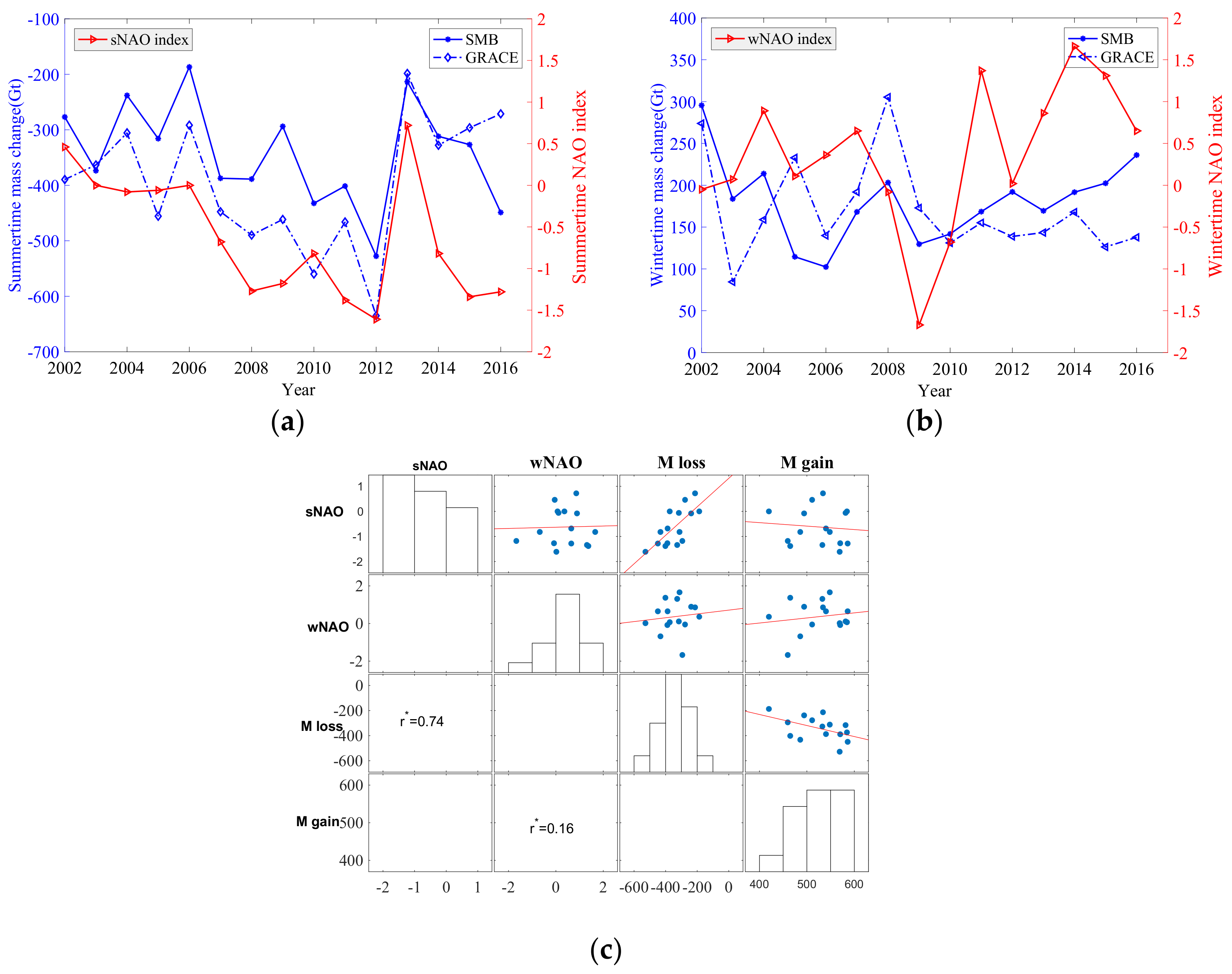
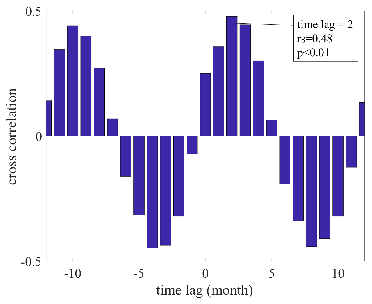
4.2.1. Connections between NAO and Mass Changes

The NAO index is an important atmospheric indicator reflecting the state of the general atmospheric circulation over Greenland. It is defined as the difference in atmospheric pressure at sea level between the Icelandic Low and the Azores High. It has been shown to be connected to extreme melting events in Greenland [63,64,65]. The positive phase of the NAO increases the accumulation at the eastern margins, which in turn, promotes the growth of glaciers, while the opposite effect occurs at the western edge. During the positive phase of the NAO, the atmospheric flow is more pronounced, and brings more moist air into Greenland’s interior. After being blocked by high-altitude glaciers, a lot of atmospheric moisture falls in the form of snow at low altitudes. Negative NAO values are associated with higher pressure and temperature over Greenland and surface melt extent and melt/runoff. The persistent anomalous ridging over Greenland is associated with persistent and anomalously negative NAO index values [66].

The correlation between the summer NAO (sNAO) index and surface temperature changes is up to −0.68 in the NO basin. The correlation between the sNAO index and the summertime precipitation is up to 0.75 in the SE basin. The correlations between the sNAO index and the summertime precipitation and 700 hPa wind profile are 0.54 and 0.55, respectively. These findings indicate that the sNAO indexes are correlated with temperature and snowfall. The NAO is most pronounced in winter, thus affecting the amount of snow accumulation in the winter [67]. For this reason, we speculate not only on the relationship between the summertime NAO index (June-July-August) and the summer mass loss in Greenland, but also between the wintertime NAO index (December-January-February) and winter snow accumulation in Greenland. As seen in Figure 6, the negative (or positive) phase of the NAO in summertime enhances (or decreases) melting over much of the Greenland, particularly in its western part (Figure 7). The summertime NAO index has a greater impact on the summer mass loss than the wintertime NAO index (wNAO) on the winter mass gain (cf. Figure 6 and Figure 7).

The larger negative phase of the sNAO index increased the prevalence of high pressure, which decreased precipitation and enhanced solar radiation, such in 2010 and 2012. The warm air migrated from the southern latitudes to west Greenland. These changes promoted higher surface temperatures and enhanced ice/snow melting. When the sNAO is positive, such as in 2013, temperatures decreased while precipitation increased, and it caused a shorter ablation season and smaller mass loss. There is a strong relation between increased mass loss and increased occurrences of the negative sNAO.

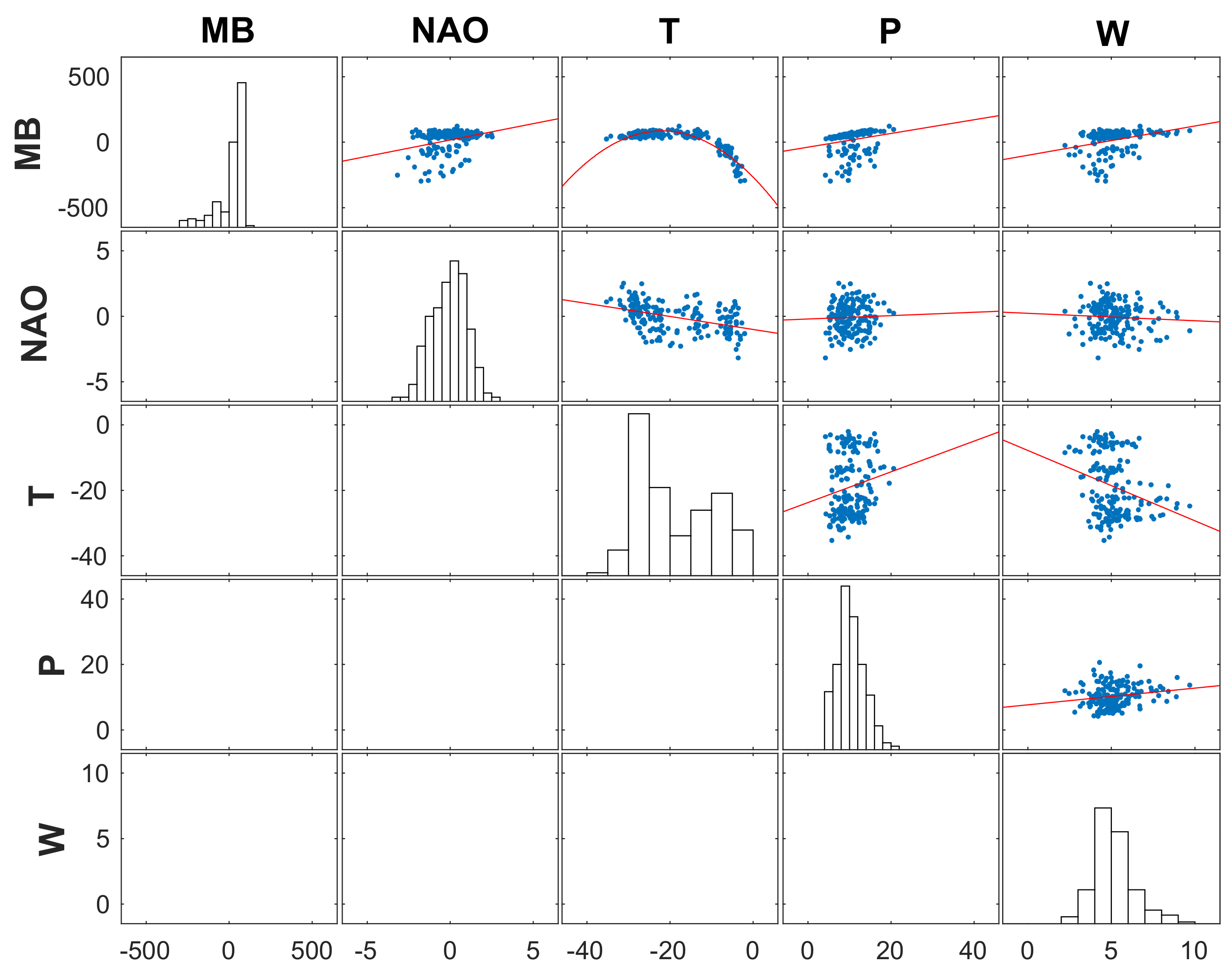
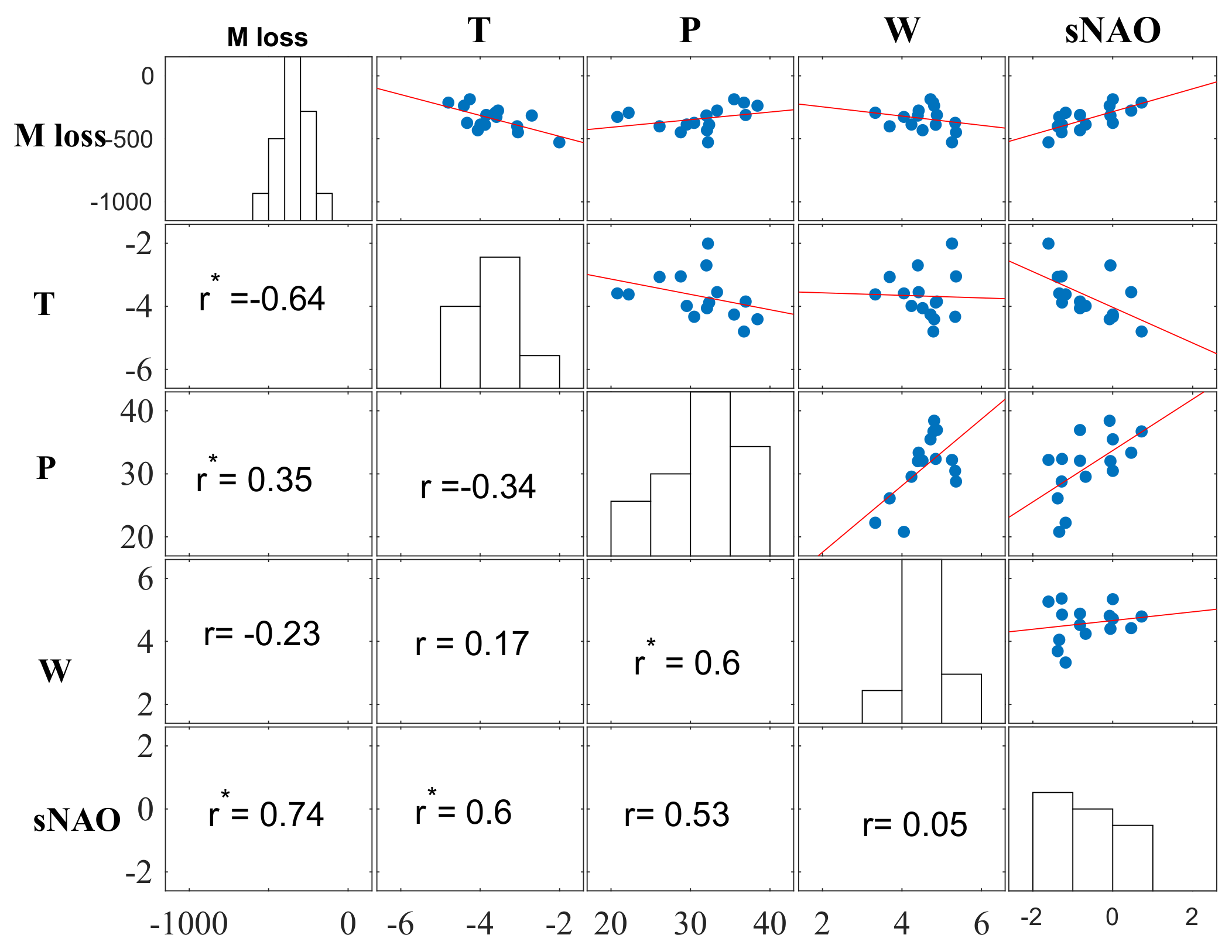
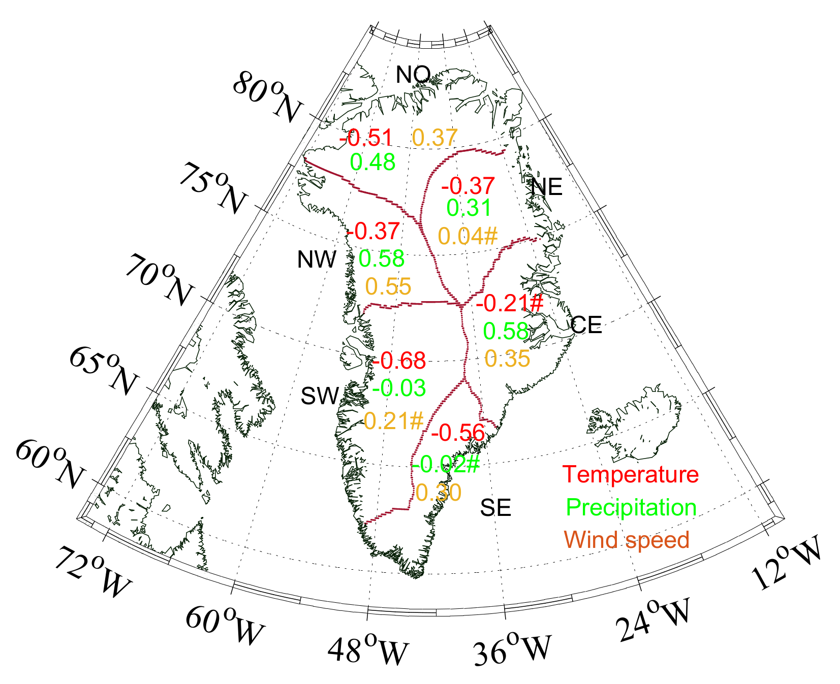
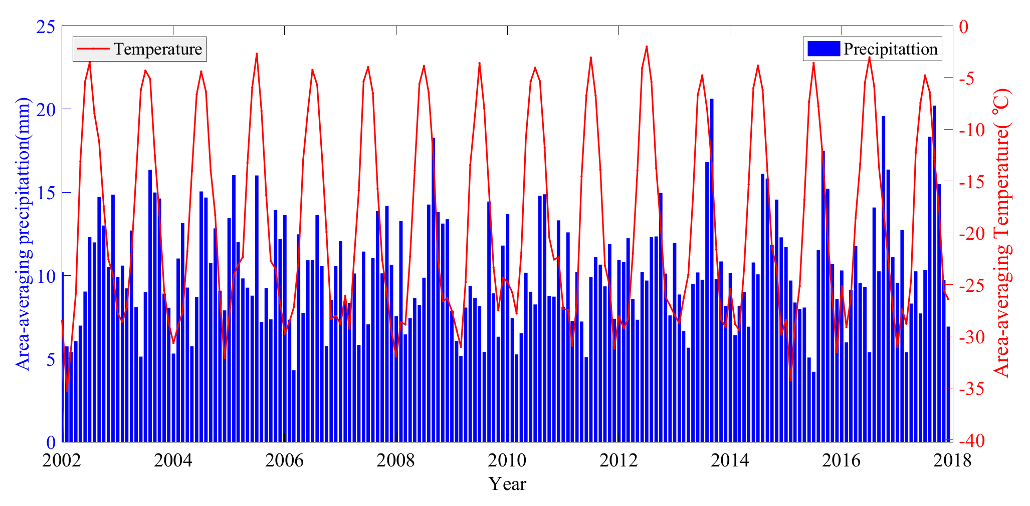
4.2.2. Relationship Between Regional Climate Controls and Mass Changes

Strong correlations between NAO and climate controls indicate that the NAO indexes are correlated with temperature, snowfall, and wind profile. NAO is a large-scale climate driver and it influences mass changes in Greenland by controlling regional temperature, precipitation, and atmospheric circulation. Although it has been reported that the GrIS mass change is correlated with the NAO, temperatures, and precipitation, the specific correlation between these climate variables and mass changes has not yet been examined. Therefore, we investigated their possible impact on the GrIS mass changes.

To quantify the relationship between climatic controls (or factors) and mass changes in the ice sheet, we correlated the time series of climate variables and mass changes (Figure 8). The surface temperature and mass changes are negatively correlated, with a moderate correlation ranging from −0.58 to −0.64. The cumulative precipitation in summer is positively correlated with mass changes (i.e., 0.33~0.35). It is important to note that the relationship between the summertime 700 hp wind speed and the summer mass change is insignificant, even failing the 90% confidence test. As wind induces precipitation, there is a positive correlation of 0.6 between the summer wind and the summer precipitation. However, it should be noted that the wind field exerts indirect control on the mass change by affecting precipitation and surface temperature.

We used the ridge regression model to estimate the summer mass loss from 2002 to 2016, while taking into consideration the summertime temperature, precipitation, wind, and NAO. We then determined the $k$ value from the ridge trace figures and obtained the regression model (for $k=0.2$ in the following form:

$$y =-229.7137-38.212\ast \mathrm{T}+3.3903\ast \mathrm{P}-69.507\ast \mathrm{W}+64.1034\ast \mathrm{NAO}$$

(12)

where $y$ denotes the summer mass change (Gt), $\mathrm{T}$ is the summer surface area-averaged temperature (°C), $\mathrm{P}$ is the summer area-averaged precipitation (mm), $\mathrm{W}$ is the summer mean wind speed (m/s), and $\mathrm{NAO}$ is the NAO index.

The p value of the t-test of this regression model is <0.01 and R² is 0.62. This indicates that 62% of the summer mass loss can be explained by climate factors. The regression also reveals that temperature and wind speed are negatively related to the summer mass changes, while precipitation and NAO are positively related. Of these, the t-test shows that the most influential variables are temperature and the NAO.

To determine a time lag between climate controls and mass changes, we analyzed the cross-correlation (in the time domain). The correlation coefficient between the surface temperature and precipitation (Figure 9) reached a maximum of 0.48 with the two-month time lag, indicating that surface temperature reached an extrema two months before the extreme precipitation. There is also a three-month time lag between precipitation and mass changes in Greenland. The correlation between the time series of mass changes from the GRACE-inferred mass loss and that of precipitation is as high as 0.68.

Figure 10 displays the correlation coefficients between climate variables and mass changes for the six drainage basins in Greenland. The surface temperature and mass changes are negatively correlated, with the largest response to temperature detected in the SW basin. The correlation between the cumulative precipitation and mass changes in the SW and SE basins is weak. A possible reason is that, in summer, these two basins have been losing their mass due to melting of surface snow and ice discharge to the extent that could not be rebalanced by precipitation. In summary, wind does not directly affect mass changes. The highest correlation (0.55) between wind speed and mass changes was found in the NW basin.

4.2.3. Associated Mechanisms

A number of authors have pointed out that the warming and persistent anomalies in the surface temperature of the GrIS are directly related to the GrIS melting [31]. We found that temperatures exceed the melting point (>0˚C) in southeast and southwest coastal regions of Greenland in the summer, particularly in July, leading to ice snow melting and glacier retreat.

Figure 11 shows the mean surface temperature and the area-averaged precipitation during the period 2002–2016. We see the highest summer temperature in 2012. Moreover, the amount of precipitation in 2013 was higher than in previous years. This explains, to a large extent, why 2013 saw a slowdown in the GrIS mass loss, with the GRACE results showing that the largest mass loss in Greenland occurred in 2012, followed by the smallest loss in 2013, while the mass loss in 2009 and 2010 was also considerable. Therefore, we selected these four years to analyze the main causes of the GrIS mass changes.

Figure 12, Figure 13 and Figure 14 illustrate the summer near-surface temperature anomalies, precipitation anomalies, and wind field anomalies, respectively, during these four years. As seen in Figure 12, the summer near-surface temperatures in 2010 and 2012 were much higher than the mean temperature over the period 2000–2016. Positive temperatures in 2010 occurred in central and south Greenland, and the maximum temperature anomalies were higher than the mean temperature in previous years by about 2 °C. In the summer of 2012, the surface temperature of the entire GrIS was significantly higher than the mean temperature over 2000–2016. The largest anomaly occurred in central Greenland (characterized by the highest elevation of the ice sheet), which was about 3 °C above the mean temperature for the study period. This temperature anomaly resulted in snow melting at the highest elevations where previously detected temperature anomalies did not reach the melting point. This caused melting in regions where mass remained stable in previous years. The area-averaged surface temperature in the SW basin even reached 1.63 °C in 2012. The average temperatures in other basins in 2012 were also the highest over the investigated period. Summer surface temperatures in 2009 and 2013 were lower than the mean summer temperature during 2000–2016, causing comparatively less summer melting in these two years (cf. Table 1). We also see that the area-averaged summer surface temperature in the NE basin reached a minimum of −3.45 °C in 2013.

As seen in Figure 13, the distribution of the summer precipitation anomalies during these four selected years is spatially more anisotropic. In general, higher precipitation occurred in the summer of 2013, and the lowest in 2009. Note that the high precipitation in the summer of 2012 exceeded expectations, being higher than the average summer precipitation over the investigated period. This also indicates that the amount of precipitation does not completely change the mass balance.

We further analyzed the effect of total precipitation on the GrIS mass changes (Figure 11). Most of the precipitation in Greenland falls as snow (~94%) and only 6% as rain [8]. Most precipitation, therefore, normally occurs from autumn to spring. Reflecting this, existing research studies have generally focused on how snow accumulation in the winter is related to precipitation (as snowfall). Our analysis, however, indicates that the amount of precipitation in the summer also affects to some extent the summer GrIS mass loss. We see, for example, that the precipitation within the SE basin exceeds all other five basins. This is due to prevailing easterly winds, frequent cyclogenesis in the region between Greenland and Iceland, and a relatively high availability of moisture from source air originating over a warmer oceans [66].

Large accumulative precipitation occurred in 2006 and 2013 in the NO basin (47.08 Gt in 2006 vs 45.28Gt in 2013) and in the NE basin (37.72 Gt in 2006 vs 36.26 Gt in 2013). This is why the speed of mass loss in these two basins slowed down sharply during 2006–2007 and 2013–2015 (Figure 4). The mass change rates even became positive, indicating an increased mass accumulation during these two periods. Periods with a lower precipitation are consistent with periods characterized by a larger mass loss. Taking the NO basin as an example, the accumulated precipitation in 2003 (28.26 Gt) and 2009 (31.66 Gt) was far lower than in other years, resulting in an obvious mass loss during these two years. A highly variable annual precipitation can partly explain fluctuations in mass changes within the NO and NE basins (Figure 4). As seen in Figure 13, the lowest amount of precipitation in the CE and SE basins occurred in 2012. After 2013, the amount of precipitation increased but remained stable. The mass loss in these two basins slowed down after 2013. The precipitation in the NW basin over the entire investigated period did not change considerably, except for the maximum precipitation that occurred in 2010.

To study the impact of atmospheric circulation on the GrIS mass changes, we analyzed the 700 hPa wind field anomalies for the four selected years. As seen in Figure 14, there was an anomalous southeast wind in south Greenland in 2009, while there was an abnormal northeast wind in north Greenland. An anomalous southerly wind in south Greenland occurred in 2010, which brought enhanced warm flow from the Atlantic Ocean, and resulted in an increased surface temperature of the ice sheet. Moreover, there was a consistent northward anomalous wind in north Greenland, bringing a considerable amount of cold air from the Arctic Ocean. This is also the reason why the surface temperature in south Greenland in 2010 was higher than during other years. Meanwhile, temperature in the south was abnormally higher than in the north.

During the summer of 2012, Greenland’s weather was significantly controlled by an anomalous anticyclone, which was not manifested over other Arctic regions, indicating a local pattern associated with the NAO. Its center was located along the southwest coast of Greenland. This period was characterized by southerly and southwesterly winds in southwest Greenland and northerly winds in its north and east parts, with the wind anomalies exceeding 4 m/s. This anticyclone anomaly facilitated the transport of heat from the northwest Atlantic Ocean through the Davis Strait to southwest of GrIS, causing a continuous melting of the ice sheet in the southwest. Melting in 2012 was also considerably higher along the west coast of Greenland as a result of the enhanced warm southerly air advection associated with an abnormal persistence of anticyclonic circulation centered in south Greenland. These findings are similar to those presented by Tedesco et al. (2013) [65].

The 700 hPa wind field anomaly exhibited an anomalous cyclone center in south and north Greenland in the summer of 2013. This anomalous cyclone can be described by the northwest wind anomaly from the Arctic in north Greenland and the northerly wind anomaly in the southwest. The cold air from the Arctic reduced the surface temperature of the GrIS, resulting in lower temperatures in northwest Greenland as well as in some parts of the southwest. There was a southerly wind anomaly along the east coast of Greenland, and a warmer airflow from the Greenland Sea increased the surface temperature of the ice sheet. The anticyclonic circulation in 2012 resulted in lower precipitation in southeast Greenland. Consequently, mass changes during autumn of 2012 were only −8.49 Gt. The anomalous cyclone in 2013 caused a larger mass loss in the autumn in southeast Greenland, up to −64.85 Gt, representing the largest mass change over the investigated period. These findings confirmed the existence of a three-month time lag between precipitation and mass changes in southeast Greenland.

5. Discussion

Our result shows that the GrIS total mass during the whole investigated period went through a rapid mass losing (2002–2008), followed by an accelerated mass loss (2009–2012), before a period of relatively slow mass loss (2013–2017). Bevis et al. (2019) observed a slow melting trend from April 2013 to 2015 after an accelerated mass loss rate −27.7 ± 4.4 Gt/yr² during 2003–2013 [1], which match well with our results. The mass changes in different drainage basins have a different change rate and fluctuation pattern due to the different regional climate pattern, especially temperature changes. The mass loss in Greenland arose due to the combination of sustained global warming and positive fluctuations in insolation, temperature, and precipitation driven by the NAO.

By analyzing the cross-correlation (in the time domain) between climate controls and mass changes, we found a three-month time lag between precipitation and mass change of the GrIS with a maximum correlation coefficient between them of up to 0.68. Taking the years 2009 vs 2010 and 2012 vs 2013 as an example, precipitation in the summer of 2012 was very rare in southeast Greenland and mass changes in the autumn of that year were very low. Higher precipitation in the summer of 2013 was accompanied by larger mass losses in the autumn in southeast Greenland. These findings indicate that larger (or lower) precipitation in the summer results in larger (or lower) mass changes in the autumn, with an apparent three-month lag. The highest precipitation occurred in September 2013 and the cumulated annual amount of precipitation after 2013 was higher than during previous years. A massive snowfall offset the GrIS mass loss, which was accompanied by a decrease in the average annual temperature, leading lead to a slower rate of mass loss after 2013.

At the regional scale, the mass changes of different basins’ behavior are likely the result of differences in ocean and atmospheric forcing. As seen in Figure 10, the surface temperature and precipitation are the most relevant climate variables to mass changes. The correlation between mass changes and climate variables in different basins are different from each other. This indicates relative uniformity in the response to changes of climate. In order to study the relationship between the surface temperature and mass changes for each basin, we plotted the summer surface temperature variations in Figure 15. Except for the CE basin, the highest summer temperatures in all basins occurred in 2012. This finding is consistent with the largest summer mass loss in 2012 as mentioned above. As seen in Figure 4 and Figure 15, the rising surface temperature during 2009–2012 in the SE and SW basins resulted in an accelerated mass loss during this period. We also see that fluctuations in mass changes (in Figure 4) and summer temperature (in Figure 15) in the SE and SW basins are highly consistent. The mass loss in the SE basin is primarily due to the increased surface melting due to short term response to climate changes [68], while the other basins were attributed to glacier dynamic and ice discharge. The ice discharge of Jakobshaven Isbra, one of largest contributors at glacier scale to sea level rise, located at the SW basin, has slowed down from ~50 Gt/yr in 2012 to ~37 Gt/yr in 2016 due to ocean cooling [61,69], and that can be seen in Figure 15, where the temperature of the SW basin since 2013 was also lower than the previous several years.

The surface temperature in the NE and NO basins had a constantly low temperature in 2006–2007, while the summer temperature in other basins was still rising at the same time. This pattern explains why the mass in the NE and NO basins showed an increasing trend at this period (Figure 4). Moreover, fluctuations in surface temperature variations in the NO and NE basins differ from those detected for the other four basins. This explains why mass change fluctuations in these two basins are different. This finding indicates that mass changes are highly related with the summer temperature. Mouginot et al. (2019) used the surface mass balance and ice discharge data and expected these two basins (NO and NE) to become of greatest importance to sea level rise due to the larger reserve of ice above sea level and the potential of the increasing in ice discharge [28].

The migration of mass including surface mass change and ice dynamic over these large scales can be detected by GRACE, and GRACE could not separate the mass changes due to these two different processes. Due to the space resolution of GRACE (330 km) and the limitation of satellite gravimetry techniques itself, the smaller scale glacier or ice dynamics cannot be easily conducted by GRACE. The surface mass balance and other ice dynamic process can be investigated by other remote sensing technique (like satellite radar ,GNSS, satellite altimetry) and in-situ observations, which could make up the shortcoming of GRACE at a small scale, such as regional and basin scale, even at glacier/ice-cap scale. In this paper, we focus on the possible impact and mechanism of climate change on the GrIS mass change over a large scale. Through studying possible impact and mechanism of climate change on mass change, we could conclude that the changes of the GrIS in the coming decades is therefore of greatest relevance to future sea level change and global water cycling as the glaciers are weakened by global and regional climate change.

6. Summary

We have estimated the GrIS mass changes based on combining the GRACE monthly solutions (over the whole period between April 2002 and June 2017) released by four different agencies in order to reduce model errors. Our result based on the GRACE time series revealed that the GrIS total mass during the study period decreased at an annual rate of −266.8 ± 32.68 Gt, with an acceleration of −12.12 ± 3.57 Gt/yr².

We applied the R package (segmented) software to analyze more realistically fluctuations and trends of mass changes of different basins in Greenland than by using only simple linear and quadratic trend estimates [1,23,70]. Our result shows that the GrIS total mass during the whole investigated period went through a rapid mass losing (2002–2008), followed by an accelerated mass loss (2009–2012), before a period of relatively slow mass loss (2013–2017).

We found that the GrIS mass changes are mostly attributed to mass loss during the summer. We demonstrated that the sensitivities of mass changes to different climate controls vary quite considerably across Greenland. The summertime NAO index is correlated with temperature, snowfall, and wind anomalies. The summertime NAO index has a greater impact on the summer mass loss than the wintertime NAO index on a winter mass gain. The negative (or positive) phase of the NAO in summer enhanced (or decreased) melting over much of Greenland, particularly in its western part. The most pronounced mass balance variations due to temperature changes are detected in the SW basin. The SE basin is characterized by the highest precipitation, while the mass balance changes in the NW basin are mostly affected by wind speed. Temperature and precipitation directly affected the GrIS mass balance, while the atmospheric circulation (wind) affects mass changes indirectly by controlling temperature and snow precipitation.

References

1. Bevis, M.; Harig, C.; Khan, S.A.; Brown, A.; Simons, F.J.; Willis, M.; Fettweis, X.; van den Broeke, M.R.; Madsen, F.B.; Kendrick, E.; et al. Accelerating changes in ice mass within Greenland, and the ice sheet’s sensitivity to atmospheric forcing. Proc. Natl. Acad. Sci. USA 2019, 116, 1934–1939. [Google Scholar] [CrossRef] [PubMed] [Green Version]
2. Chen, J.L.; Wilson, C.R.; Tapley, B.D. Contribution of ice sheet and mountain glacier melt to recent sea level rise. Nat. Geosci. 2013, 6, 549–552. [Google Scholar] [CrossRef]
3. Graversen, R.G.; Drijfhout, S.; Hazeleger, W.; Wal, R.V.D.; Bintanja, R.; Helsen, M. Greenland’s contribution to global sea-level rise by the end of the 21st century. Clim. Dyn. 2011, 37, 1427–1442. [Google Scholar] [CrossRef] [Green Version]
4. Jacob, T.; Wahr, J.; Pfeffer, W.T.; Swenson, S. Recent contributions of glaciers and ice caps to sea level rise. Nature 2012, 482, 514–518. [Google Scholar] [CrossRef] [PubMed]
5. Rignot, E.; Velicogna, I.; Broeke, M.R.V.D.; Monaghan, A.; Lenaerts, J.T.M. Acceleration of the contribution of the Greenland and Antarctic ice sheets to sea level rise. Geophys. Res. Lett. 2011, 38. [Google Scholar] [CrossRef] [Green Version]
6. Slater, D.A.; Felikson, D.; Straneo, F.; Goelzer, H.; Nowicki, S. Twenty-first century ocean forcing of the Greenland ice sheet for modelling of sea level contribution. Cryosphere 2020, 14, 985–1008. [Google Scholar] [CrossRef] [Green Version]
7. Chambers, D.P. Calculating trends from GRACE in the presence of large changes in continental ice storage and ocean mass. Geophys. J. Int. 2009, 176, 415–419. [Google Scholar] [CrossRef] [Green Version]
8. Ettema, J.; van den Broeke, M.R.; van Meijgaard, E.; van de Berg, W.J.; Bamber, J.L.; Box, J.E.; Bales, R.C. Higher surface mass balance of the Greenland ice sheet revealed by high-resolution climate modeling. Geophys. Res. Lett. 2009, 36. [Google Scholar] [CrossRef] [Green Version]
9. Simpson, M.J.R.; Wake, L.; Milne, G.A.; Huybrechts, P. The influence of decadal- to millennial-scale ice mass changes on present-day vertical land motion in Greenland: Implications for the interpretation of GPS observations. JGR 2011, 116. [Google Scholar] [CrossRef] [Green Version]
10. Wahr, J.; Khan, S.A.; van Dam, T.; Liu, L.; van Angelen, J.H.; van den Broeke, M.R.; Meertens, C.M. The use of GPS horizontals for loading studies, with applications to northern California and southeast Greenland. J. Geophys. Res. Solid Earth 2013, 118, 1795–1806. [Google Scholar] [CrossRef] [Green Version]
11. Bolch, T.; Sandberg Sørensen, L.; Simonsen, S.B.; Mölg, N.; Machguth, H.; Rastner, P.; Paul, F. Mass loss of Greenland’s glaciers and ice caps 2003–2008 revealed from ICESat laser altimetry data. Geophys. Res. Lett. 2013, 40, 875–881. [Google Scholar] [CrossRef] [Green Version]
12. Ewert, H.; Groh, A.; Dietrich, R. Volume and mass changes of the Greenland ice sheet inferred from ICESat and GRACE. J. Geodyn. 2012, 59–60, 111–123. [Google Scholar] [CrossRef]
13. Slobbe, D.C.; Ditmar, P.; Lindenbergh, R.C. Estimating the rates of mass change, ice volume change and snow volume change in Greenland from ICESat and GRACE data. Geophys. J. Int. 2009, 176, 95–106. [Google Scholar] [CrossRef] [Green Version]
14. Helm, V.; Humbert, A.; Miller, H. Elevation and elevation change of Greenland and Antarctica derived from CryoSat-2. Cryosphere 2014, 8, 1539–1559. [Google Scholar] [CrossRef] [Green Version]
15. Su, X.; Shum, C.K.; Guo, J.; Duan, J.; Howat, I.; Yi, Y. High resolution Greenland ice sheet inter-annual mass variations combining GRACE gravimetry and Envisat altimetry. Earth Planet. Sci. Lett. 2015, 422, 11–17. [Google Scholar] [CrossRef]
16. Chen, J.L.; Wilson, C.R.; Tapley, B.D. Satellite gravity measurements confirm accelerated melting of Greenland ice sheet. Science 2006, 313, 1958–1960. [Google Scholar] [CrossRef]
17. Jin, S.; Zou, F. Re-estimation of glacier mass loss in Greenland from GRACE with correction of land–ocean leakage effects. Glob. Planet. Chang. 2015, 135, 170–178. [Google Scholar] [CrossRef]
18. Ran, J.; Ditmar, P.; Klees, R. Optimal mascon geometry in estimating mass anomalies within Greenland from GRACE. Geophys. J. Int. 2018, 214, 2133–2150. [Google Scholar] [CrossRef]
19. Weigelt, M.; van Dam, T.; Jäggi, A.; Prange, L.; Tourian, M.J.; Keller, W.; Sneeuw, N. Time-variable gravity signal in Greenland revealed by high-low satellite-to-satellite tracking. J. Geophys. Res. Solid Earth 2013, 118, 3848–3859. [Google Scholar] [CrossRef] [Green Version]
20. Baur, O.; Kuhn, M.; Featherstone, W.E. GRACE-derived ice-mass variations over Greenland by accounting for leakage effects. JGR 2009, 114. [Google Scholar] [CrossRef] [Green Version]
21. Luthcke, S.B.; Sabaka, T.J.; Loomis, B.D.; Arendt, A.A.; McCarthy, J.J.; Camp, J. Antarctica, Greenland and Gulf of Alaska land-ice evolution from an iterated GRACE global mascon solution. J. Glaciol. 2017, 59, 613–631. [Google Scholar] [CrossRef]
22. Schrama, E.J.O.; Wouters, B.; Rietbroek, R. A mascon approach to assess ice sheet and glacier mass balances and their uncertainties from GRACE data. J. Geophys. Res. Solid Earth 2014, 119, 6048–6066. [Google Scholar] [CrossRef]
23. Velicogna, I.; Sutterley, T.C.; van den Broeke, M.R. Regional acceleration in ice mass loss from Greenland and Antarctica using GRACE time-variable gravity data. Geophys. Res. Lett. 2014, 41, 8130–8137. [Google Scholar] [CrossRef] [Green Version]
24. Bamber, J.L.; Baldwin, D.J.; Gogineni, S.P. A new bedrock and surface elevation dataset for modelling the Greenland ice sheet. Ann. Glaciol. 2017, 37, 351–356. [Google Scholar] [CrossRef] [Green Version]
25. Noel, B.; Fettweis, X.; Van de Berg, W.; Van Den Broeke, M.; Erpicum, M. Sensitivity of Greenland Ice Sheet surface mass balance to perturbations in sea surface temperature and sea ice cover: A study with the regional climate model MAR. Cryosphere 2014, 8, 1871–1883. [Google Scholar] [CrossRef] [Green Version]
26. Noël, B.; van de Berg, W.J.; Machguth, H.; Lhermitte, S.; Howat, I.; Fettweis, X.; van den Broeke, M.R. A daily, 1 km resolution data set of downscaled Greenland ice sheet surface mass balance (1958–2015). Cryosphere 2016, 10, 2361–2377. [Google Scholar] [CrossRef] [Green Version]
27. Van den Broeke, M.; Box, J.; Fettweis, X.; Hanna, E.; Noël, B.; Tedesco, M.; van As, D.; van de Berg, W.J.; van Kampenhout, L. Greenland ice sheet surface mass loss: Recent developments in observation and modeling. Curr. Clim. Chang. Rep. 2017, 3, 345–356. [Google Scholar] [CrossRef] [Green Version]
28. Mouginot, J.; Rignot, E.; Bjørk, A.A.; Michiel, V.D.B.; Millan, R.; Morlighem, M.; Noël, B.; Scheuchl, B.; Wood, M. Forty-six years of Greenland Ice Sheet mass balance from 1972 to 2018. Proc. Natl. Acad. Sci. USA 2019, 116, 9239–9244. [Google Scholar] [CrossRef] [Green Version]
29. Zou, F.; Tenzer, R.; Fok, H.S.; Nichol, J.E. Mass Balance of the Greenland Ice Sheet from GRACE and Surface Mass Balance Modelling. Water 2020, 12, 1847. [Google Scholar] [CrossRef]
30. Hall, D.K.; Williams, R., Jr.; Casey, K.; Digirolamo, N.E.; Wan, Z. Satellite-derived, melt-season surface temperature of the Greenland Ice Sheet (2000–2005) and its relationship to mass balance. Geophys. Res. Lett. 2006, 33. [Google Scholar] [CrossRef] [Green Version]
31. Tedesco, M.; Serreze, M.; Fettweis, X. Diagnosing the extreme surface melt event over southwestern Greenland in 2007. Cryosphere Discuss. 2008, 2, 383–397. [Google Scholar] [CrossRef] [Green Version]
32. Seo, K.-W.; Waliser, D.E.; Lee, C.-K.; Tian, B.; Scambos, T.; Kim, B.-M.; van Angelen, J.H.; van den Broeke, M.R. Accelerated mass loss from Greenland ice sheet: Links to atmospheric circulation in the North Atlantic. Glob. Planet. Chang. 2015, 128, 61–71. [Google Scholar] [CrossRef]
33. Box, J. Greenland ice sheet surface mass-balance variability: 1991–2003. Ann. Glaciol. 2005, 42, 90–94. [Google Scholar] [CrossRef]
34. Murphy, B.F.; Marsiat, I.; Valdes, P. Atmospheric contributions to the surface mass balance of Greenland in the HadAM3 atmospheric model. J. Geophys. Res. Atmos. 2002, 107, ACL 3-1–ACL 3-20. [Google Scholar] [CrossRef]
35. Bezeau, P.; Sharp, M.; Gascon, G. Variability in summer anticyclonic circulation over the Canadian Arctic Archipelago and west Greenland in the late 20th/early 21st centuries and its effect on glacier mass balance. Int. J. Climatol. 2015, 35, 540–557. [Google Scholar] [CrossRef]
36. Fettweis, X.; Hanna, E.; Lang, C.; Belleflamme, A.; Erpicum, M.; Gallée, H. Important role of the mid-tropospheric atmospheric circulation in the recent surface melt increase over the Greenland ice sheet. Cryosphere 2013, 7, 241–248. [Google Scholar] [CrossRef] [Green Version]
37. Hanna, E.; Fettweis, X.; Mernild, S.H.; Cappelen, J.; Ribergaard, M.H.; Shuman, C.A.; Steffen, K.; Wood, L.; Mote, T.L. Atmospheric and oceanic climate forcing of the exceptional Greenland ice sheet surface melt in summer 2012. Int. J. Climatol. 2014, 34, 1022–1037. [Google Scholar] [CrossRef] [Green Version]
38. Sakumura, C.; Bettadpur, S.; Bruinsma, S. Ensemble prediction and intercomparison analysis of GRACE time-variable gravity field models. Geophys. Res. Lett. 2014, 41, 1389–1397. [Google Scholar] [CrossRef]
39. Wahr, J.; Molenaar, M.; Bryan, F. Time variability of the Earth’s gravity field: Hydrological and oceanic effects and their possible detection using GRACE. J. Geophys. Res. Solid Earth 1998, 103, 30205–30229. [Google Scholar] [CrossRef]
40. Swenson, S.; Chambers, D.; Wahr, J. Estimating geocenter variations from a combination of GRACE and ocean model output. J. Geophys. Res. Solid Earth 2008, 113. [Google Scholar] [CrossRef] [Green Version]
41. Cheng, M.; Tapley, B.D.; Ries, J.C. Deceleration in the Earth’s oblateness. J. Geophys. Res. Solid Earth 2013, 118, 740–747. [Google Scholar] [CrossRef]
42. Swenson, S.; Wahr, J. Post-processing removal of correlated errors in GRACE data. Geophys. Res. Lett. 2006, 33. [Google Scholar] [CrossRef]
43. Archie, P.; Shijie, Z.; John, W. Inference of mantle viscosity from GRACE and relative sea level data. Geophys. J. Int. 2007, 171, 492–508. [Google Scholar]
44. A, G.; Wahr, J.; Zhong, S. Computations of the viscoelastic response of a 3-D compressible Earth to surface loading: An application to Glacial Isostatic Adjustment in Antarctica and Canada. Geophys. J. Int. 2013, 192, 557–572. [Google Scholar] [CrossRef]
45. Khan, S.A.; Sasgen, I.; Bevis, M.; Van Dam, T.; Bamber, J.L.; Wahr, J.; Willis, M.; Kjaer, K.H.; Wouters, B.; Helm, V. Geodetic measurements reveal similarities between post–Last Glacial Maximum and present-day mass loss from the Greenland ice sheet. Sci. Adv. 2016, 2, e1600931. [Google Scholar] [CrossRef] [PubMed] [Green Version]
46. Fleming, K.; Lambeck, K. Constraints on the Greenland Ice Sheet since the Last Glacial Maximum from sea-level observations and glacial-rebound models. Quat. Sci. Rev. 2004, 23, 1053–1077. [Google Scholar] [CrossRef]
47. Fleming, K.; Martinec, Z.; Hagedoorn, J. Geoid displacement about Greenland resulting from past and present-day mass changes in the Greenland Ice Sheet. Geophys. Res. Lett. 2004, 31. [Google Scholar] [CrossRef] [Green Version]
48. Peltier, W.R. GLOBAL GLACIAL ISOSTASY AND THE SURFACE OF THE ICE-AGE EARTH: The ICE-5G (VM2) Model and GRACE. Annu. Rev. Earth Planet. Sci. 2004, 32, 111–149. [Google Scholar] [CrossRef]
49. Slangen, A.; Katsman, C.; Van de Wal, R.; Vermeersen, L.; Riva, R. Towards regional projections of twenty-first century sea-level change based on IPCC SRES scenarios. Clim. Dyn. 2012, 38, 1191–1209. [Google Scholar] [CrossRef] [Green Version]
50. Karegar, M.A.; Dixon, T.H.; Malservisi, R.; Kusche, J.; Engelhart, S.E. Nuisance flooding and relative sea-level rise: The importance of present-day land motion. Sci. Rep. 2017, 7, 1–9. [Google Scholar] [CrossRef] [Green Version]
51. NOAA. North Atlantic Oscillation (NAO). Available online: https://www.ncdc.noaa.gov/teleconnections/nao/ (accessed on 15 May 2020).
52. Olauson, J. ERA5: The new champion of wind power modelling? Renew. Energy 2018, 126, 322–331. [Google Scholar] [CrossRef] [Green Version]
53. Massey, E.J. The Kolmogorov-Smirnov Test of Goodness of Fit. J. Am. Stat. Assoc. 1951, 46. [Google Scholar] [CrossRef]
54. Gauthier, T.D. Detecting Trends Using Spearman’s Rank Correlation Coefficient. Environ. Forensics 2001, 2, 359–362. [Google Scholar] [CrossRef]
55. Ni, S.; Chen, J.; Wilson, C.R.; Li, J.; Hu, X.; Fu, R. Global Terrestrial Water Storage Changes and Connections to ENSO Events. Surv. Geophys. 2018, 39, 1–22. [Google Scholar] [CrossRef]
56. Saleh, A.K.M.E.; Kibria, B.M.G. Performance of some new preliminary test ridge regression estimators and their properties. Commun. Stat. Theory Methods 1993. [Google Scholar]
57. Hoerl, A.E.; Kennard, R.W. Ridge Regression: Applications to Nonorthogonal Problems. Technometrics 1970, 12, 69–82. [Google Scholar] [CrossRef]
58. Muggeo, V.M. Segmented: An R package to fit regression models with broken-line relationships. R News 2008, 8, 20–25. [Google Scholar]
59. Muggeo, V.M. Estimating regression models with unknown break-points. Stat. Med. 2003, 22, 3055–3071. [Google Scholar] [CrossRef]
60. Gladish, C.V.; Holland, D.M.; Rosing-Asvid, A.; Behrens, J.W.; Boje, J. Oceanic Boundary Conditions for Jakobshavn Glacier. Part I: Variability and Renewal of Ilulissat Icefjord Waters, 2001–14. J. Phys. Oceanogr. 2015, 45, 3–32. [Google Scholar] [CrossRef] [Green Version]
61. Khazendar, A.; Fenty, I.G.; Carroll, D.; Gardner, A.; Lee, C.M.; Fukumori, I.; Wang, O.; Zhang, H.; Seroussi, H.; Moller, D. Interruption of two decades of Jakobshavn Isbrae acceleration and thinning as regional ocean cools. Nat. Geosci. 2019, 12, 277. [Google Scholar] [CrossRef]
62. Zwally, H.J.; Giovinetto, M.B.; Beckley, M.A.; Sab, J.L. Antarctic and Greenland Drainage Systems. Available online: http://icesat4.gsfc.nasa.gov/cryo_data/ant_grn_drainage_systems.php (accessed on 3 January 2020).
63. Sodemann, H.; Schwierz, C.; Wernli, H. Interannual variability of Greenland winter precipitation sources: Lagrangian moisture diagnostic and North Atlantic Oscillation influence. J. Geophys. Res. Atmos. 2008, 113. [Google Scholar] [CrossRef] [Green Version]
64. Bevis, M.; Wahr, J.; Khan, S.A.; Madsen, F.B.; Brown, A.; Willis, M.; Kendrick, E.; Knudsen, P.; Box, J.E.; van Dam, T. Bedrock displacements in Greenland manifest ice mass variations, climate cycles and climate change. Proc. Natl. Acad. Sci. USA 2012, 109, 11944–11948. [Google Scholar] [CrossRef] [PubMed] [Green Version]
65. Tedesco, M.; Fettweis, X.; Mote, T.; Wahr, J.; Alexander, P.; Box, J.; Wouters, B. Evidence and analysis of 2012 Greenland records from spaceborne observations, a regional climate model and reanalysis data. Cryosphere 2013, 7, 615–630. [Google Scholar] [CrossRef] [Green Version]
66. Berdahl, M.; Rennermalm, A.; Hammann, A.; Mioduszweski, J.; Hameed, S.; Tedesco, M.; Stroeve, J.; Mote, T.; Koyama, T.; Mcconnell, J.R. Southeast Greenland Winter Precipitation Strongly Linked to the Icelandic Low Position. J. Clim. 2018, 31, 4483–4500. [Google Scholar] [CrossRef]
67. Mosley-Thompson, E.; Readinger, C.; Craigmile, P.; Thompson, L.; Calder, C. Regional sensitivity of Greenland precipitation to NAO variability. Geophys. Res. Lett. 2005, 32. [Google Scholar] [CrossRef] [Green Version]
68. King, M.D.; Howat, I.M.; Candela, S.G.; Noh, M.J.; Negrete, A. Dynamic ice loss from the Greenland Ice Sheet driven by sustained glacier retreat. Commun. Earth Environ. 2020, 1. [Google Scholar] [CrossRef]
69. Mankoff, K.D.; Colgan, W.; Solgaard, A.; Karlsson, N.B.; Ahlstrøm, A.P.; Van As, D.; Box, J.E.; Khan, S.A.; Kjeldsen, K.K.; Mouginot, J. Greenland Ice Sheet solid ice discharge from 1986 through 2017. Earth Syst. Sci. Data 2019, 11, 769–786. [Google Scholar] [CrossRef] [Green Version]
70. Sasgen, I.; van den Broeke, M.; Bamber, J.L.; Rignot, E.; Sørensen, L.S.; Wouters, B.; Martinec, Z.; Velicogna, I.; Simonsen, S.B. Timing and origin of recent regional ice-mass loss in Greenland. Earth Planet. Sci. Lett. 2012, 333–334, 293–303. [Google Scholar] [CrossRef] [Green Version]
Figure 1. (a). The topography of Greenland. The black lines delineate the boundaries of each discharge basin discussed in the text. (b). The drainage basins and definitions of the Greenland Ice Sheet (GrIS) for Gravity Recovery and Climate Experiment (GRACE).
Remotesensing 12 03250 g001
Figure 2. The Glacial Isostatic Adjustment rates in the GrIS according to the GIA model prepared by Geruo et al. (2013) (in terms of the equivalent water thickness, cm/yr).
Remotesensing 12 03250 g002
Figure 3. GrIS mass changes from GRACE between April 2002 and June 2017 after applying the forward modeling technique to suppress the ocean–land leakage effect.
Remotesensing 12 03250 g003
Figure 4. Mass changes in the drainage basins (see Figure 1) (a) NO, (b) NE, (c) CE, (d) SE, (e) SW, and (f) NW estimated based on averaging the GRACE monthly solutions from four processing centers between April 2002 and June 2017 with a forward modeling technique applied to suppress the ocean–land leakage effect.
Remotesensing 12 03250 g004aRemotesensing 12 03250 g004b
Figure 5. Scatterplots between mass changes (MB) and the investigated climate factors; North Atlantic Oscillation (NAO), T (temperature), P (precipitation), and W (wind).
Remotesensing 12 03250 g005
Figure 6. Interannual mass changes from GRACE compared with the (a) summertime (June-July-August) NAO index (sNAO) and (b) wintertime (December-January-February) NAO index (wNAO). (c) The correlation of the NAO index and mass changes inferred from GRACE. The M_loss is the summertime mass loss from GRACE, and the M_gain is the wintertime mass gain from GRACE (the correlations r * are computed at the 95% confidence levels, p < 0.05).
Remotesensing 12 03250 g006
Figure 7. Correlations between the NAO index and mass changes for the six drainage basins in Greenland. Red values represent the correlation between the summertime NAO (sNAO) index and the summertime mass changes in each basin, and blue values represent the correlation between the wintertime NAO (wNAO) index and the wintertime mass changes from GRACE. The correlation values with # represent the significant value p > 0.05.
Remotesensing 12 03250 g007
Figure 8. Correlation of the summer NAO index and the summertime mass losses from the GRACE products. The correlation r* represents the p-value < 0.05, and the correlation r indicates the p-value >0.05.
Remotesensing 12 03250 g008
Figure 9. Correlations between the temperature and precipitation time series changes with changing time lag. The correlations are computed at the 99% confidence levels.
Remotesensing 12 03250 g009
Figure 10. Correlation coefficients of climate variables and mass changes for the six basins of Greenland. Red values represent the correlation between the surface temperature and mass changes, green values represent the correlation between the cumulative precipitation and mass changes, and orange values represent the correlation between the 700 hPa wind speed and mass changes. All correlations with # represent p value > 0.05.
Remotesensing 12 03250 g010
Figure 11. Time series of the mean surface temperature and the area-averaged precipitation during 2002–2016 (temperature unit: °C, precipitation unit: mm).
Remotesensing 12 03250 g011
Figure 12. Summer near-surface temperature anomalies (relative to the average over 2000–2016) in: (a) 2009, (b) 2010, (c) 2012, and (d) 2013.
Remotesensing 12 03250 g012
Figure 13. Summer precipitation anomalies (relative to the average over the period 2000-2016) in: (a) 2009, (b) 2010, (c) 2012, and (d) 2013.
Remotesensing 12 03250 g013
Figure 14. Summer wind anomalies in: (a) 2009, (b) 2010, (c) 2012, and (d) 2013.
Remotesensing 12 03250 g014
Figure 15. Time series of the summer near-surface temperatures for the six basins in Greenland.
Remotesensing 12 03250 g015