Coastal Erosion and Human Perceptions of Revetment Protection in the Lower Meghna Estuary of Bangladesh

Abstract

This study investigates coastal erosion, revetment as a shoreline protection strategy, and human perceptions of revetments in the Lower Meghna estuary of the Bangladesh where new revetments were recently constructed. Questions addressed were: (1) How do rates of shoreline change vary over the period 2011–2019? (2) Did new revetments effectively halt erosion and what were the magnitudes of erosion change? (3) How have erosion rates changed for shorelines within 1 km of revetments, and (4) How do households perceive revetments? High-resolution Planet Lab imagery was used to quantify shoreline change rates. Analysis of household survey data assessed human perceptions of the revetment’s desirability and efficacy. Results revealed high rates of erosion for 2011–2019 with declining erosion after 2013. New revetments effectively halted erosion for protected shorelines. Significant spatial trends for erosion rates existed for shorelines adjacent to revetments. Survey respondents overwhelmingly had positive attitudes about a desire for revetment protection; however, upstream respondents expressed a strong majority perception that revetment acts to make erosion worse. Highlights of the research include integration of remote sensing with social science methods, the timing of the social survey shortly after revetment construction, and results showing significant erosion change upstream and downstream of new revetments.

1. Introduction

Globally, coastal areas are vulnerable to a variety of natural hazards that include floods, cyclones, hurricanes, tsunami, saltwater intrusion, and coastal erosion. These hazards are responsible for extensive human, financial, social, and ecological disturbances [1]. Climate change and sea-level rise are projected to increase the vulnerability of the people living in the coastal regions and global mega deltas [2,3]. Coastal erosion is one of the most prominent problems in the coastal areas including global mega deltas [4]. According to IPCC, sea level has risen 10–20 cm during the 20th century, possibly exacerbating coastal erosion globally [5]. In coastal areas, land reclamation and shoreline protection are mitigative strategies to save the coastal lands and infrastructure [6,7]. Quantification of erosion/accretion and the effects of shoreline protection is particularly important to manage coastal land and formulate policies and plans to mitigate coastal erosion. Time-series remote sensing approaches have emerged as an effective approach for analysis of shoreline change detection drawing from 30+ years of satellite images available via Google Earth engine [8,9]. Other platforms delivering higher resolution imagery have become increasingly available for coastal analysis. Additionally, geospatial softwares such as the Digital Shoreline Analysis System (DSAS) [10] exist to enable robust quantification of shoreline change rates. Several hundred peer-reviewed articles have used DSAS (described below) in empirical studies.

This research investigates the spatio-temporal variation in shoreline change and the erosion mitigation effects of newly introduced concrete revetments along the east bank of the Lower Meghna estuary of Bangladesh, located at the coastal outlet of the Ganges-Brahmaputra-Meghna (GBM) delta. The GBM drainage basin covers all of Bangladesh and encompasses all or part of India, China, Bhutan, and Myanmar. Over 90% of GBM discharge flows through Bangladesh to the Bay of Bengal with a large majority flowing out of the Lower Meghna estuary. The GBM delta is the largest among the highly populated Asian mega deltas covering an estimated area of more than 100,000 km² [4]. This delta is among the world’s most dynamic due to coastal processes and annual monsoon rainfall that yields tremendous discharge driving erosion and accretion processes [11,12,13]. Discharge is heavily influenced by seasonality, with 80% of the annual discharge occurring during the four months of the southwestern monsoon season [14].

Coastal Bangladesh experiences erosion and accretion rates that are among the highest in the world [15,16,17]. Coastal erosion in Bangladesh is a recurring problem, causing thousands of people to be displaced annually. Economically challenged populations experience significant vulnerability and chronic erosion-induced displacement. The magnitude and severity of affected peoples have negative consequences for national economic vitality and growth [18]. Erosion causes population displacement and associated loss of economically productive land area, infrastructure, communication systems, and household livelihoods. As a developing country with limited internal resources, Bangladesh is particularly at a challenge to cope with coastal shoreline erosion and its negative consequences [19].

To protect coastal agricultural land and communities, the government of Bangladesh initiated construction of coastal embankments in the 1960s as part of the Coastal Embankment Plan (CEP) [20,21]. The CEP established a system of polders where the land is surrounded by earthen embankments for flood protection and with drainage weirs to manage water levels enhancing agricultural activities [22]. 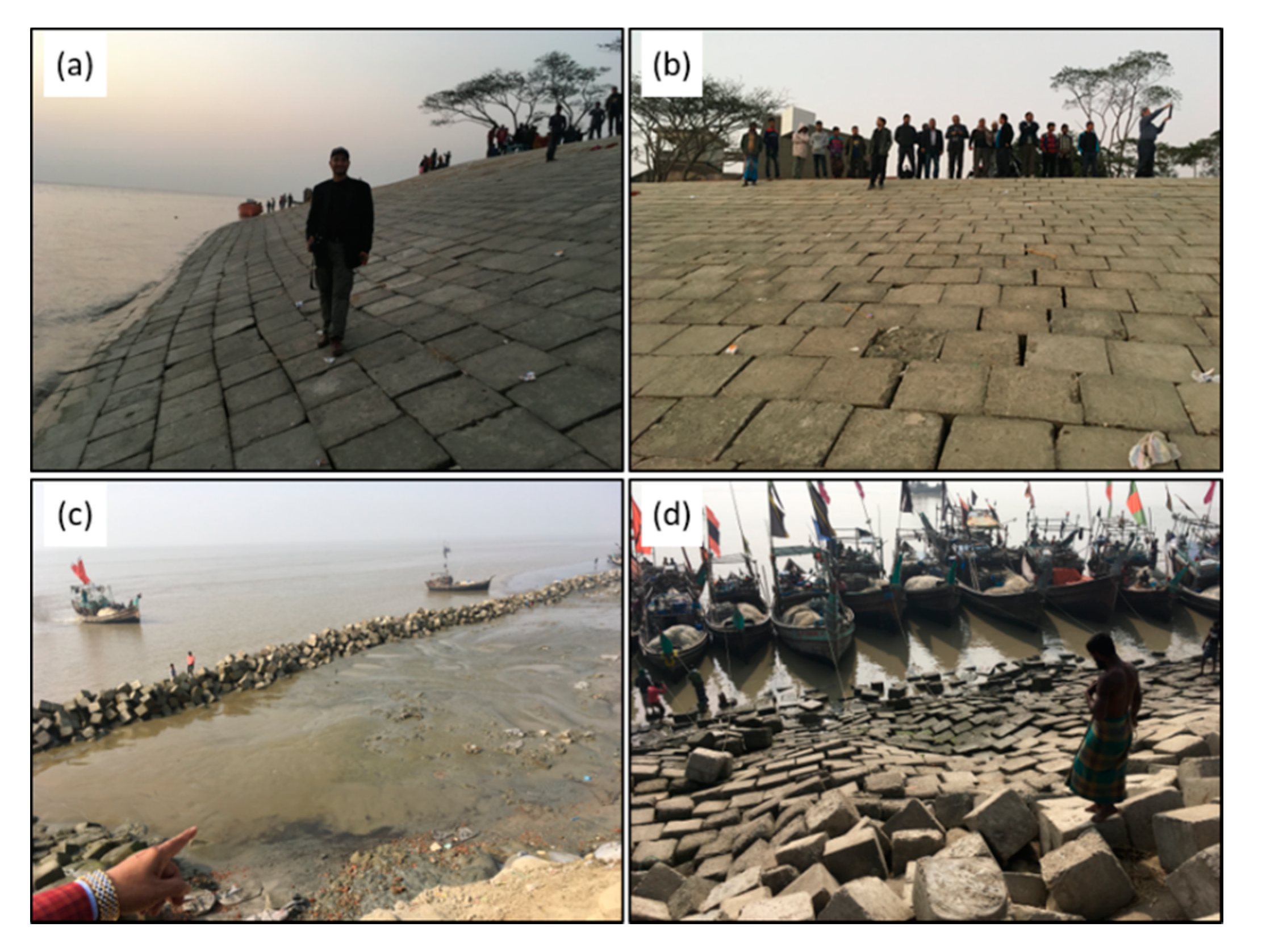In the decades since the initiation of the CEP, concrete revetments have been constructed along many of Bangladesh’s coastal shorelines [23]. These revetment structures are commonly constructed of concrete blocks at a sloped angle as opposed to vertical concrete seawalls. The sloped nature of revetments act to more effectively protect shorelines and interior land by absorbing and dissipating more energy compared to vertical seawalls (Figure 1). Both revetments and seawalls are prone to scour at the base of the structure due to reflected wave energy and turbulence, though revetments suffer less of this structural weakening effect compared to vertical seawalls due to their better ability to dissipate hydrodynamic energy [24,25]. Additionally, both revetments and seawalls can experience flanking erosion at their terminal ends [26,27] whereby reflected water flow and wave energy causes erosion for unprotected shorelines adjacent to the structures. Further, downdrift sites can experience heightened erosion due to sediment deficit caused by coastal protective defenses [28,29,30].

Remote sensing and GIS techniques are useful and widely used by coastal researchers in detecting coastal erosion and accretion throughout the world [16,23,31]. In Bangladesh, a substantial literature has quantified riverbank erosion patterns for non-coastal, interior regions (e.g., Jamuna and Padma rivers) [32,33] as well as for the exterior coastal region facing the Bay of Bengal [23,34] using remotely sensed imagery. Though much of the shoreline change research uses Landsat imagery, this research has used much finer resolution data from Planet Labs to quantify rates of shoreline change.

Table 1. Selected coastal erosion rates from different delta and coastal regions.

Reference	Region	Temporal Resolution	Spatial Resolution	Coastal Change Rates
Bangladesh Coast
Sarwar and Woodroffe 2013 [23]	Bangladesh	10 years	30 m	−35 to −285 m/y
Islam et al., 2016 [35]	Bangladesh	4 years	30, 60 m	0 to −100 m/y
Salauddin et al., 2018 [36]	Bangladesh	5 years	30 m	−3 to −130 m/y
Other Delta Regions
Dada et al., 2016 [37]	Niger R. delta	5,10 years	30 m	−4 to −30 m/y
Ghoneim et al., 2015 [38]	Nile R. delta	2 years	1.84, 57 m	−30 m/y
Esmail et al., 2019 [39]	Nile R. delta	10 years	15, 30 m	−5 to −70 m/y
Zhang et al., 2018 [40]	Yellow R. delta	20 years	30, 60 m	−25 to −35 m/y
Qiao et al., 2018 [41]	Yangtze R. delta	5 years	1.8, 30 m	−30 m/y
Indian Coast
Jana et al., 2014 [42]	India coast	10 years	30, 60 m	−1 to −10 m/y
Natesan et al., 2015 [43]	India coast	10 years	30, 60 m	−7 to −40 m/y
Rani et al., 2018 [44]	India coast	10 years	30 m	−2 to −80 m/y
Baral et al., 2018 [45]	India coast	3 years	23.5, 60 m	−1 to −10 m/y
Jayanthi et al., 2017 [46]	India coast	10 years	30, 60 m	0 to −55 m/y

summarizes selected literature on shoreline change research on delta and coastal regions in Bangladesh and other parts of the world. These studies reveal that coastal Bangladesh has among the highest erosion rates in the world.

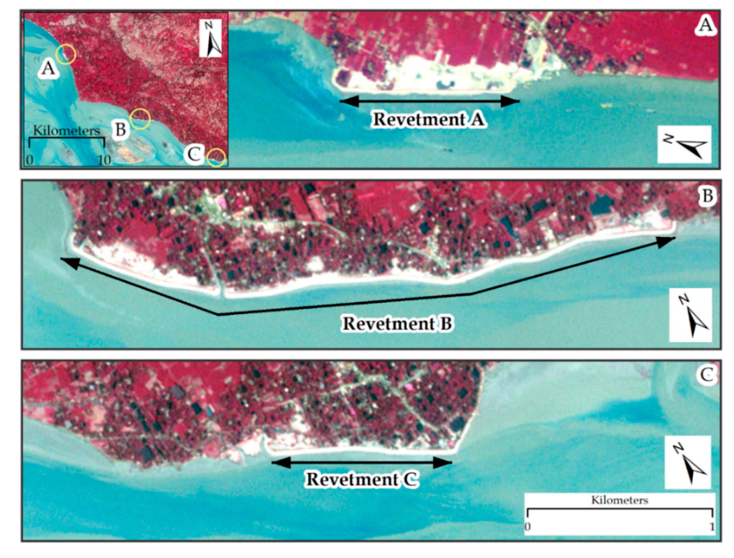
This study investigates shoreline erosion patterns for the southern portion of Lakshmipur District in Kamalnagar and Ramgati Upazilas, which prior research has identified as having high erosion rates [17]. These sites had no presence of concrete revetment protection until recent years when three revetments were constructed in protecting a relatively small portion of the shoreline (Figure 2). A northern revetment, Revetment A, was initiated in 2017 in Kamalnagar with a length of approximately 0.9 km completed in 2018. A centrally located revetment, Revetment B, was initiated in 2015 in Ramgati with about 3.2 km in length completed in 2017. A third revetment, Revetment C, was initiated in the far southern reach of Ramgati in 2018 and is not included in the analysis due to its newness with respect to imagery available for meaningful change analysis. The combined 4.2 km length of Revetments A and B used for analysis protects approximately 11% of the total 38 km shoreline length of the combined Kamalnagar and Ramgati shoreline.

A goal of this research is to quantify the effects of two of these new revetments on mitigating erosion as well as to assess erosion patterns for non-protected proximal shorelines. We also introduce human dimension perspectives by assessment, for a region containing Revetment B, household perceptions regarding revetment construction and efficacy. We analyzed data from a household survey in Ramgati conducted in April–May of 2018 following the 2015–2017 construction period of Revetment B. GPS household location points were collected for each household. The spatial nature of our household data relative to the location of Revetment B offers opportunities to assess household perceptions of revetment protection depending on if households are in locations that are protected or unprotected by this new revetment. The timing of the survey is such that results reveal perceptions for a period very soon after the revetment was completed. We specify the following research questions.

Research Objectives and Questions:

Q1. How do rates of shoreline change vary over the period 2011–2019 for Kamalnagar and Ramgati Upazilas?

Q2. Did new revetments effectively halt erosion, and what were the magnitudes of erosion change?

Q3. For each of the two new revetments, how have erosion rates changed for shorelines proximal to the terminal ends of the revetments for the periods after the revetments were completed?

Q4. Are there differences in how households perceive the desirability and efficacy of engineered revetments depending on if they are located in regions that are protected or unprotected by new revetments?

2. Materials and Methods

2.1. Study Area

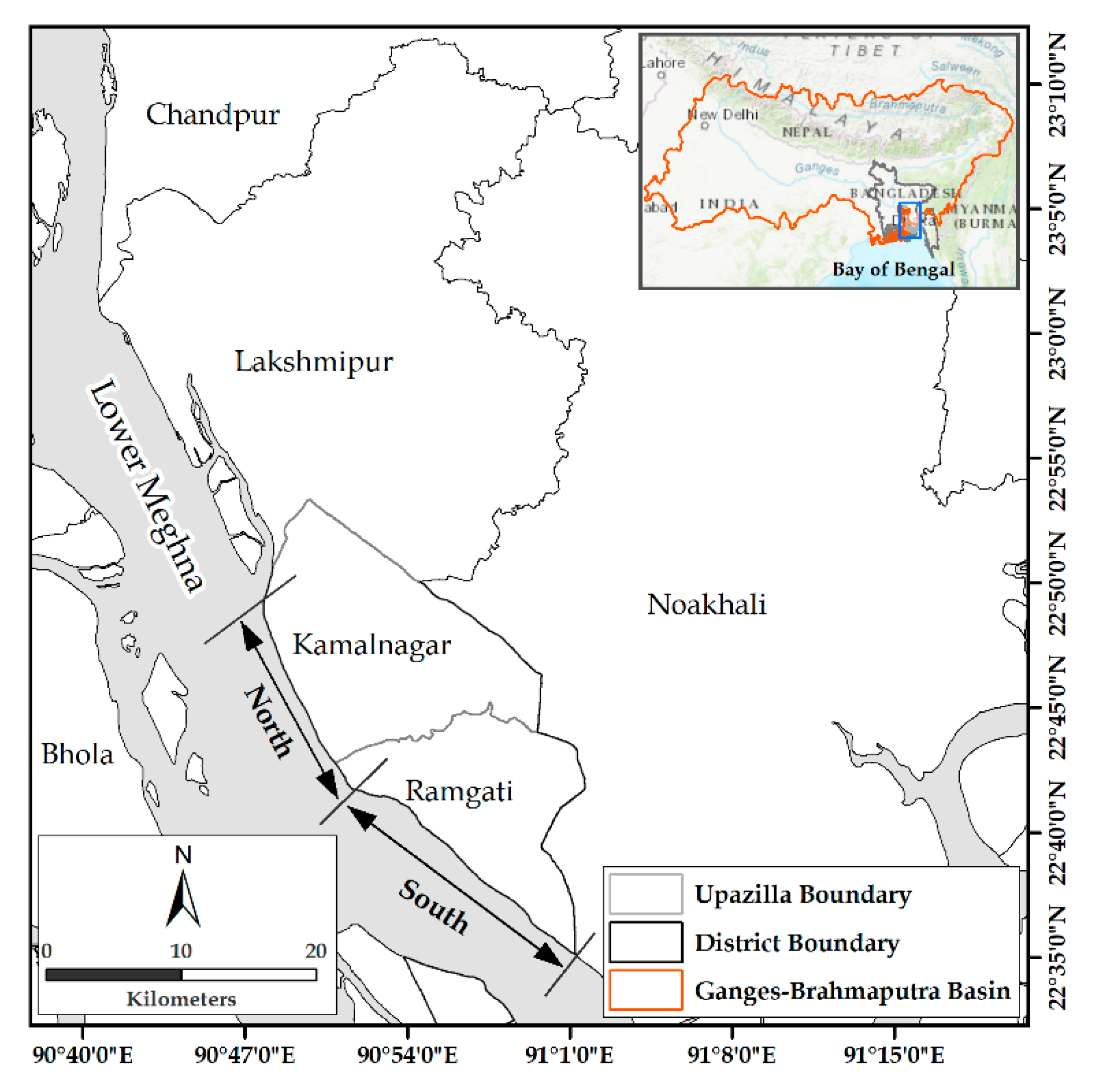
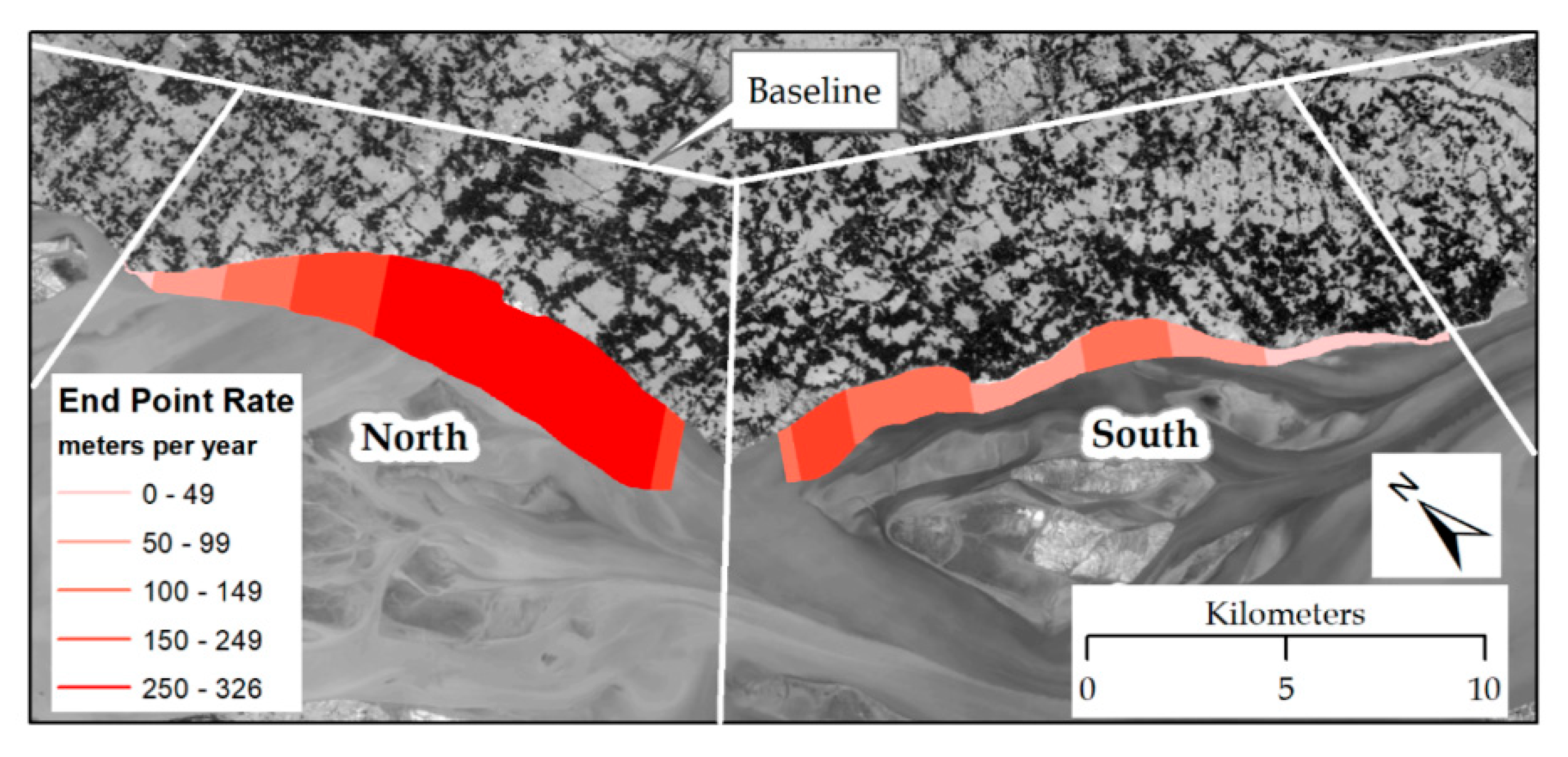
The study area is located in Ramgati and Kamalnagar Upazilas within Lakshmipur District (Figure 3). According to the most recent 2011 Bangladesh census, the combined population of these two upazilas was 483,917. Using the WorldPop 100 m resolution gridded population dataset [47], we estimate that 135,362 of the Upazilas’ population (28.0%) lived within 3 km of the 2011 Lower Meghna estuary shoreline. In Bangladesh, of the highest body of the local government administration is a district containing Upazilas, which is composed of Unions comprising approximately ten villages. For census enumeration and government elections, the Union is the smallest administrative unit, though population refers colloquially to a home village. For presentation, we divide our focal shoreline that fronts Kamalnagar and Ramgati into North and South regions respectively, which we refer to later. Our household survey contains data predominantly from the South region in Ramgati Upazila. A small number of sampled households were located in Kamalnagar Upazila located slightly north of the South region.

2.2. Satellite Imagery

Satellite imagery used in this study (

Table 2. Imagery used to estimate End Point Rate (EPR) and Linear Regression Rate (LRR).

Image Source	Image Date	Representative Dry Season Year	Resolution
RapidEye	29 October 2010	2011	6.5 m
RapidEye	13 November 2011	2012	6.5 m
RapidEye	6 February 2013	2013	6.5 m
RapidEye	12 November 2013; 1 January 2014	2014	6.5 m
RapidEye	16 November 2014; 22 November 2014	2015	6.5 m
RapidEye	20 November 2015; 23 November 2015	2016	6.5 m
PlanetScope	9 December 2016; 4 January 2017	2017	3.7 m
PlanetScope	4 December 2017; 24 December 2017	2018	3.7 m
PlanetScope	6 January 19; 17 January 2019	2019	3.7 m

Note: All images were used to estimate LRR. Images for the 2011 and 2019 and incremental pairs of dry season years were used to estimate EPR.

) was obtained from Planet Lab, a US commercial imaging company [48]. Planet Lab’s RapidEye and PlanetScope image data with a resolution of 6.5 m and 3.7 m respectively were processed to generate representative annual dry-season shorelines from 2011 to 2019. In other regions, this spatial resolution would not be sufficient to resolve annual change. However, the high rate of change in this study area enables appropriate use of the Planet Lab imagery. For our purposes, shorelines would ideally be derived from January or February anniversary dates situated temporally in the middle of the monsoonal dry season. Based on the availability of cloud-free and dry season imagery, we selected the best available images representing dry season anniversary dates. It is noted that these dates are not real anniversaries so that, for example, a November 2011 image was used that represented the 2012 dry-season shoreline. In one case, a late October 2010 image was used that represented the 2011 dry-season shoreline. This approach is justified because the majority of erosion occurs during the June–September monsoon period. It is important to note that the method of describing the erosion rate uses exact image dates to calculate shoreline change by normalizing actual inter-image duration to yield rates in units of meters per year. We refer to erosion rates even though accretion can occur. We do so because erosion is the overwhelming shoreline response in the study area [17]. Shoreline change rates were estimated using both the End Point Rate (EPR) and Linear Regression Rate (LRR) and described below.

2.3. Shoreline Extraction

Alternative remote sensing indices exist to aid shoreline extraction. The Normalized Difference Water Index (NDWI) is one of the most widely used indices [49,50,51]. Other indices such exist such as the Modified Normalized Difference Water Index (MNDWI) and Automated Water Extraction Index (AWEI) required MIR and SWIR bands. The Planet Lab imagery used here did not contain MIR/SWIR bands so that use of MNDWI or AWEI was not possible. To enhance extraction of annual shorelines, we calculated the Normalized Difference Water Index (NDWI), which makes use of the green and near-infrared (NIR) bands [52]. NDWI values can range from −1 to 1, with water pixels typically being greater than zero and approaching 1 for clear open water.

$$\mathrm{NDWI}=\frac{\mathrm{Green}-\mathrm{NIR}}{\mathrm{Green}+\mathrm{NIR}}$$

(1)

Planet Lab imagery and the derived NDWI band were used as input to define shorelines. The task of separating water from land in this setting with discrete shorelines on the mainland is justified. Much other research extracts shorelines via visual digitization. We believe our approach is suitable and enables replication. The ISODATA unsupervised classification method using NDWI and Red, Green, Blue, and NIR (near infrared) bands was employed in ArcGIS to classify this bandset into ten output classes that were then reclassified into two classes, water and non-water. Geospatial processing methods converted this output into preliminary vector GIS shorelines. Vector GIS editing methods including visual inspection and treatment of small tributary gaps transformed the preliminary shorelines into final annual shorelines used for analysis.

Shoreline uncertainty was assessed and accounts for four uncertainty terms: Ug georeferencing uncertainty, Up pixel uncertainty, Ud digitizing uncertainty, and Ut uncertainty associated with tidal variation [53]. Georeferencing uncertainty (Ug) of the Planet Labs imagery is stated as <10 m RMSE by Planet Labs. We use the 10 m RMSE as the maximum digitizing uncertainty for all shorelines. Pixel uncertainty (Up) is defined by the pixel resolution of the respective imagery. Digitizing uncertainty (Ud) is typically associated with manual digitizing of shorelines from visual inspection of source imagery (e.g., heads up digitizing). With this method, multiple analysts digitize the same shoreline, and uncertainty is quantified. With our method of automated shoreline digitization, the same shorelines will result with multiple shoreline generation so that Ud = 0. Uncertainty due to tidal variation (Ut) was assessed in the following manner. We used six Landsat images during the representative dry season of 2000 and applied our automated methodology to derive six shorelines. While the use of higher resolution Planet Lab imagery for the same years of analysis is desirable, their use was not feasible due to cost consideration. This approach of using Landsat-derived shorelines provides a justifiable estimate of tidal uncertainty. Tidal levels ranged from 0.8 m to 2.8 m for the dates/times of the analyzed images at a nearby tidal station. All inter-shoreline distances for the 15 combinations of shorelines for each transect were quantified to measure how shoreline position differs depending on the tidal level. The mean tidal difference was 0.97 m across all combinations. Regression analysis revealed that shoreline uncertainty exhibits a relationship of 7 m shoreline shift per 1 m tidal difference. We assume that the mean tidal difference is 1 m so that we apply a tidal uncertainty of Ut = 7.0 m. The total uncertainty for each shoreline position (Utotal) is stated by the following equation and specific shoreline uncertainties are stated in

Table 3. Shoreline uncertainty.

Shoreline Year	Ug	Up	Ud	Ut	Utotal
2011–2016 1	10 m	6.5 m	0.0 m	7.0 m	13.8 m
2017–2019 2	10 m	3.7 m	0.0 m	7.0 m	12.7 m

Utotal = total shoreline uncertainty, Ug = digitizing uncertainty, Up = pixel uncertainty, Ud = digitizing uncertainty, Ut = tidal uncertainty. ¹ Uncertainty for each annual shoreline 2011–2016. ² Uncertainty for each annual shoreline 2017–2019.

. Uncertainties are generally on par with though slightly larger than the ~10 m horizontal accuracy associated with the CoastSat toolkit [8] which draws from a 30-year times series of publicly available imagery. The high rates of erosion (revealed below) relative to spatial uncertainty justify our use of the Planet Lab imagery.

$$\mathrm{Utotal}=\sqrt{{\mathrm{Ug}}^2+{\mathrm{Up}}^2+{\mathrm{Ud}}^2+{\mathrm{Ut}}^2}$$

(2)

Further assessment of shoreline accuracy was performed by comparing the shorelines derived from Planet Lab imagery with shoreline positions obtained from reference images in Google Earth Pro. Reference image dates were determined using this application’s historical imagery tool. Only reference images within two months of images used for shoreline mapping were deemed acceptable. For some years, there were no reference images meeting this criterion so that assessment is possible only for the years shown in

Table 4. Shoreline accuracy using Google Earth reference images.

Representative Dry Season Year	Number of Observations	RMSE
2012	35	14.8 m
2013	47	7.2 m
2016	68	14.7 m
2017	42	13.4 m
2019	36	13.9 m
All years	228	13.1 m

Google Earth reference images not available for years 2011, 2014, 2015, 2018.

. For each year, every 10th DSAS transect was overlaid in Google Earth and transect-shoreline points were obtained via heads up digitizing. Resulting reference x,y coordinates were integrated with x,y coordinates of assessed shorelines to calculate RMSE. The number of observations varies by year due to local scale image availability at appropriate dates along with cloud cover, which made it impossible to obtain reference points for every sample transect. Results indicate reference accuracies on par with shoreline uncertainties in Table 3 and that the derived shorelines are suitable to assess shoreline change in this study area, which has erosion rates at much higher magnitudes.

2.4. Shoreline Change Estimation

Shoreline change rates were estimated using the Digital Shoreline Analysis System (DSAS) [10]. The DSAS software is widely used in research and consists of three key components (Figure 4): (1) a user-defined baseline running parallel to the shoreline and located either offshore or onshore, (2) a set of digital transects cast orthogonal from the baseline, and (3) transect-specific quantification of shoreline movement rates based on inter-shoreline distances of shoreline positions obtained from transect-shoreline intersection points. A total of 633 transects were created at 50 m increments (

Table 5. Transect and shoreline parameters used for shoreline change analysis.

Parameter	North	South	All
Number of transects *	292	341	633
# of transects intersecting new revetment	19	64	83
Length of analyzed shoreline (km) **	14.6 km	17.0 km	31.6 km
Length of shoreline protected by revetment (km)	0.9 km	3.2 km	4.1 km
% of shoreline protected by new revetment **	6.2%	18.8%	13.0%

* Digital transects spaced at 50 m intervals were cast using DSAS shoreline change software in ArcGIS. ** Analyzed shoreline was 31.6 km, which does not include all of the 38 km shoreline for Kamalnagar and Ramgati Upazilas.

).

We initially used both End Point Rate (EPR) and Linear Regression Rate (LRR) within DSAS. Both are commonly used in the research literature [23,54,55,56]. The End Point Rate (EPR) is calculated by dividing the distance of shoreline movement by the years elapsed between shoreline dates.

$$\mathrm{EPR}\left(\mathrm{m}/\mathrm{year}\right)=\frac{\mathrm{Shoreline}\mathrm{movement}\mathrm{from}\mathrm{A}\mathrm{to}\mathrm{B}\left(\mathrm{m}\right)}{\mathrm{Years}\mathrm{duration}\mathrm{from}\mathrm{A}\mathrm{to}\mathrm{B}\left(\mathrm{yr}\right)}$$

(3)

where A = the start image data and B = the terminal image date. Erosion is reported as positive valued EPR throughout.

The Linear Regression Rate (LRR) is estimated by fitting a least-squares regression line for each transect where y = distance along a transect from the baseline to observed transect-shoreline intersections, and x = shoreline date. LRR is the regression slope obtained for each transect and is an estimated rate of shoreline movement (erosion or accretion) along the transect in meters per year. By using annual shorelines for the period 2011 to 2019, each transect had eight (x,y) observations input into LRR regression estimation. For clarity of presentation, we present results only from EPR due to the high Pearson’s correlation between EPR and LRR of 0.996.

As stated above, we organized our transect data into two regions, North and South (Figure 3). It was based on results from the Grouping Analysis tool of ArcGIS [57]. This method groups spatial observations into clusters using a spatially explicit K-means method based on feature location and a quantitative feature attribute. The features were the 633 transects and the attribute was the transect EPR. Results revealed an optimal grouping (clustering) into the North and South regions indicated by pseudo F-statistics generated from successive groupings of 2 to 15 clusters. This two-cluster result accords well visually and quantitatively with observations of higher erosion rates in Kamalnagar Upazila (North) that differed from rates in Ramgati Upazila (South).

2.5. Social Survey

The combined use of remote sensing data with social survey data allows us to integrate human dimensions with geophysical dimensions of shoreline change in a spatially explicit manner. This approach is consistent with research linking “people and pixels” that investigates landscape change involving both social and biophysical domains [58,59,60]. From April to June of 2018, a household survey was conducted in a set of coastal villages located primarily in the South region within Ramgati Upazila. We selected households using a random spatial sampling design with a higher sampling intensity for near shoreline areas to adequately capture perceptions of population most at risk of shoreline erosion. An initial set of 420 random latitude/longitude points was generated using GIS software and plotted on large format field maps to aid field navigation and household recruitment. Two project leaders coordinated a set of six data enumerators to recruit household respondents (one respondent per household) and to complete a household survey instrument. Enumerators navigated to the random point locations and approached the nearest household for recruitment. If a household declined participation, the next nearest household was invited to participate. All human subject activities were approved by the Institutional Review Board (IRB) of the Virginia Polytechnic Institute and State University (Virginia Tech). The survey contained questions spanning multiple topics with a focus on erosion hazards and took approximately one hour to complete. The present analysis draws on the following Likert-scale questions addressing perceptions of riverbank erosion risk and revetment protection:

Perception of embankment protection:

• How do you agree that, “an engineered revetment should be constructed to protect the Meghna River shoreline of my union”?
• How you agree that, “an engineered revetment should be constructed to protect the entire Meghna River shoreline from my union all the way to Chandpur approximately 100 km north of here”?
• How do you agree that, “I think the revetment construction in recent years near my area is a positive thing”?
• How do you agree that, “I think the revetment acts to protect areas near the revetment but acts to make riverbank erosion worse for other areas that are not protected by the revetment”?

A 5-point Likert scale was used for these survey questions ranging from strongly agree to strongly disagree. For analysis, responses were aggregated to a 3-point scale of agree, neutral, and disagree.

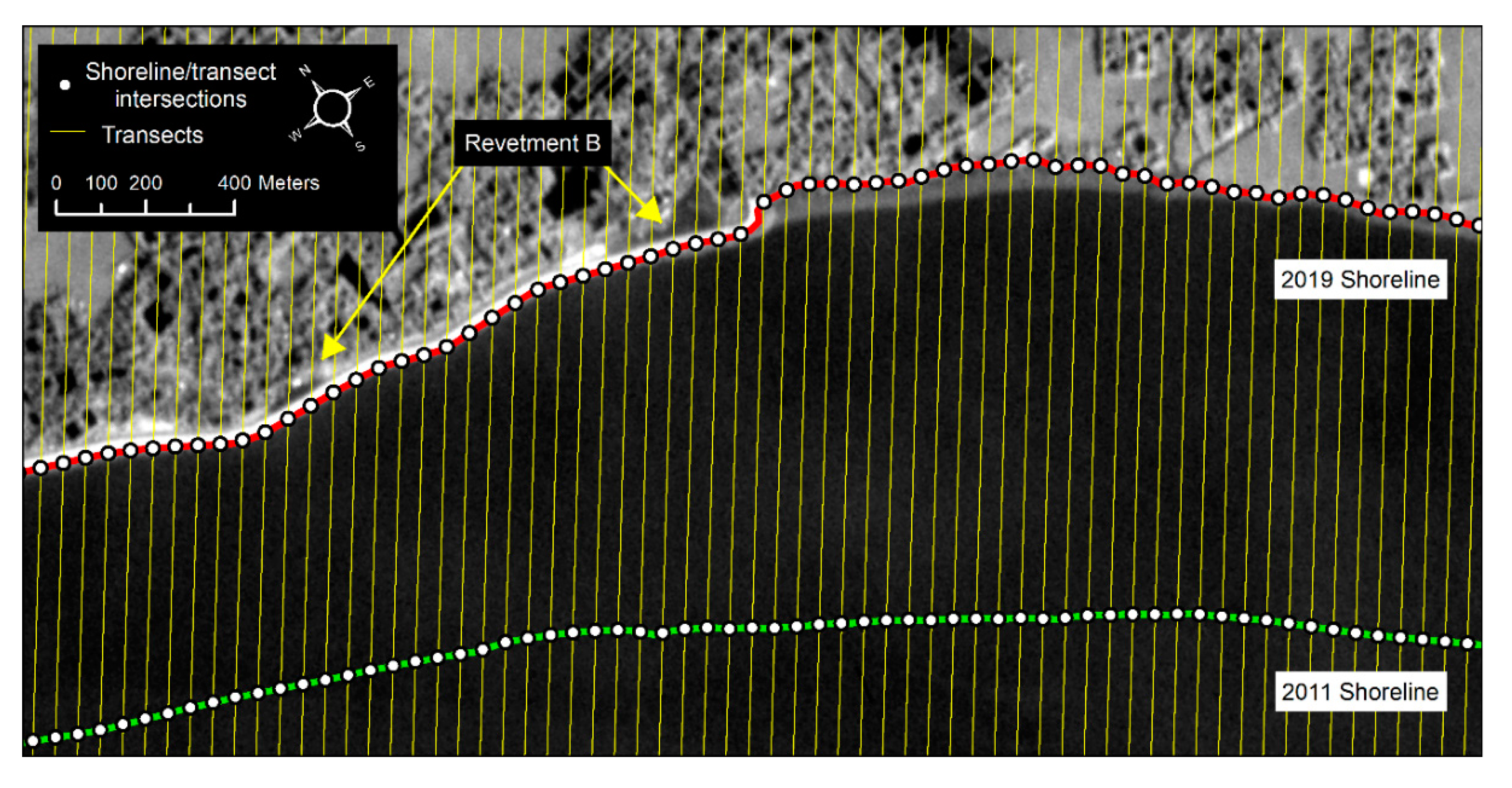
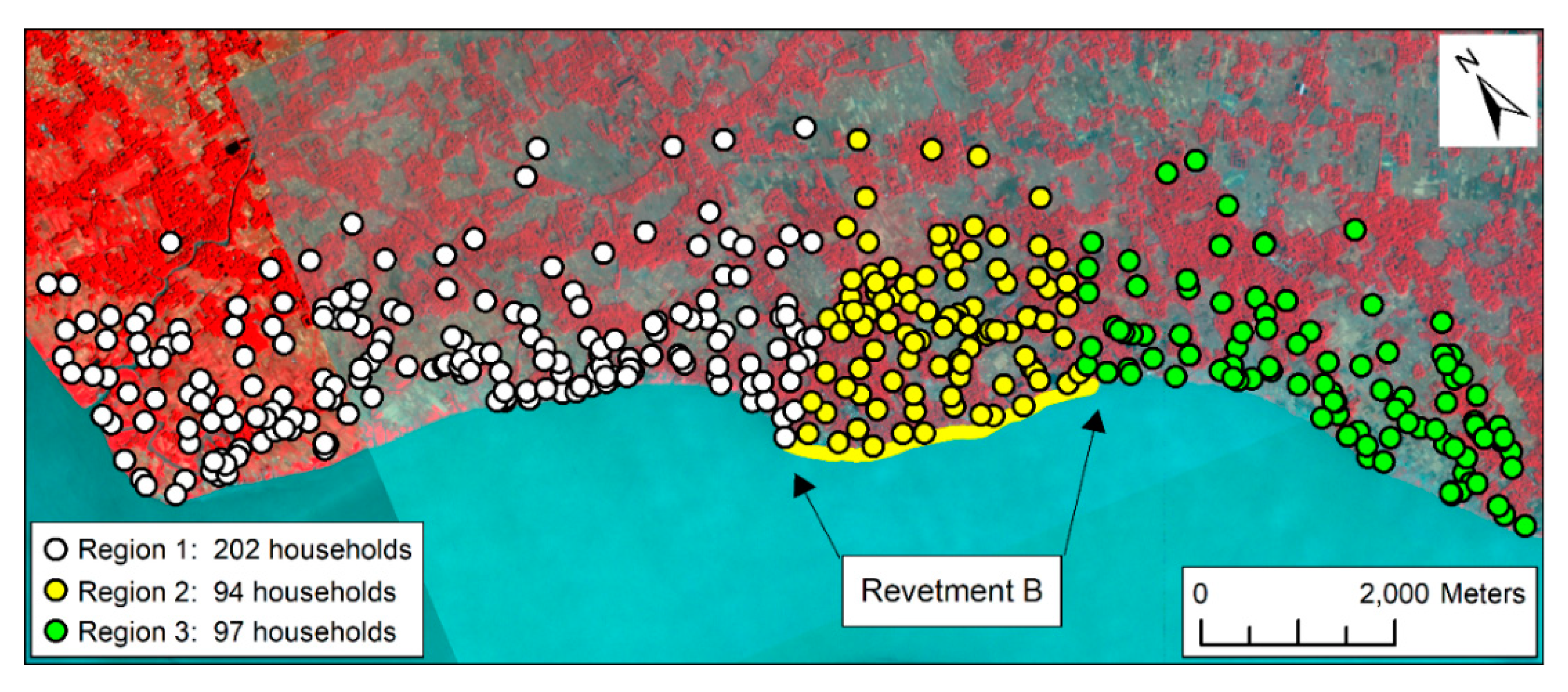
The 3.2 km Revetment B in Ramgati was constructed starting in 2015 and completed in 2017. Its central location within our social survey area enables analysis and comparison of response differences depending on household locations and their protection status due to the revetment. We defined households into three regions visually by inspecting household locations relative to the revetment and shoreline (Figure 5). Region 1 households upstream of the Revetment B have no revetment protection. Region 2 households are fronted by the new Revetment B, which offers protection from riverbank erosion. Region 3 households downstream of Revetment B have no revetment protection.

For survey Questions 1–3 (see above), results are presented for all survey respondents. For Question 4 which focuses on the near-revetment effects on erosion, only the n = 88 responses for households located within 1 km of the 2018 shoreline, located (and protected) behind the revetment, and located within 1 km upstream or downstream of the revetment are reported. These 88 households were selected due to their likely heightened perceptions of erosion patterns for shorelines most near the revetment.

Appendix A (

Table A1. Socio-economic characteristics of household respondents.

		Region 1	Region 2	Region 3	All Regions
Gender	Male	116	59	72	247
		58.3%	63.4%	75.8%	63.8%
	Female	83	34	23	140
		41.7%	36.6%	24.2%	36.2%
	Total	199	93	95	387
		100.0%	100.0%	100.0%	100.0%
Education	Elementary	143	52	61	256
level		73.0%	57.1%	64.9%	67.2%
	High school	29	25	17	71
		14.8%	27.5%	18.1%	18.6%
	College/university/higher	12	10	12	34
		6.1%	11.0%	12.8%	8.9%
	None	12	4	4	20
		6.1%	4.4%	4.2%	5.2%
	Total	196	91	94	381
		100.0%	100.0%	100.0%	100.0%
Occupation	Farming	50	23	42	115
of hh head		24.8%	24.5%	43.3%	29.3%
	Fishing	49	8	4	61
		24.3%	8.5%	4.1%	15.5%
	Farming and fishing	17	3	6	26
		8.4%	3.2%	6.2%	6.6%
	Small business/service	54	42	25	121
		26.7%	44.7%	25.8%	30.8%
	Other	32	18	20	70
		15.8%	19.1%	20.6%	17.8%
	Total	202	94	97	393
		100.0%	100.0%	100.0%	100.0%

and

Table A2. Age, residency, and distance characteristics of household respondents and households.

		Region 1	Region 2	Region 3	All Regions
Age in years of respondent	N	200	94	97	391
	Mean	44.85	43.32	44.91	44.91
	Std dev.	14.28	15.50	15.95	14.99
Months residency in	N	200	94	96	390
current house	Mean	24.54	26.35	30.68	26.49
	Std dev.	20.38	22.77	22.32	21.44
Months residency in	N	178	88	95	361
current union	Mean	36.81	39.81	41.57	38.79
	Std dev.	17.78	20.22	18.78	18.72
Distance in meters from	N	202	94	97	393
house to Meghna shoreline	Mean	733.25	1080.80	676.27	802.32
	Std dev.	581.00	652.19	507.51	601.71

) describes selected socio-economic and spatial characteristics of sampled households included in analysis (n = 393). For some measures, the number of total responses is less than 393 due to missing data when respondents did not answer a question.

2.6. Analysis Methods

Q1. How do rates of shoreline change vary over the period 2011–2019 for Kamalnagar and Ramgati Upazilas?

Thematic mapping and descriptive statistics summarized the End Point Rate of shoreline erosion comparing the North (Kamalnagar) and South (Ramgati) regions during the 2011–2019 period. The Student’s t-test was used to determine if there were significant differences in mean EPR between North and South. Erosion rates are also reported for each successive one-year duration of shoreline change from 2011–2019.

Q2. Did new revetments effectively halt erosion and what were the magnitudes of erosion change?

EPR was estimated for shorelines derived for before/after periods of revetment installation (

Table 6. Planet Lab imagery used to estimate End Point Rate (EPR) before and after installation of revetments.

New Revetment	Before/After	Start Image Dates	End Image Dates	Representative Dry Season Years
A	Before	16 November 2014; 22 November 2014	9 December 2016; 4 January 2017	2015–2017
A	After	9 December 2016; 4 January 2017	6 January 2019; 17 January 2019	2017–2019
B	Before	29 October 2010	16 November 2014; 22 November 2014	2011–2015
B	After	16 November 2014; 22 November 2014	6 January 2019; 17 January 2019	2015–2019

). Before/after periods for Revetment A were 2015–2017 and 2017–2019. Before/after periods for Revetment B were 2011–2015 and 2015–2019. These dates were selected in order to have the same time duration for both periods with respect to each revetment. Transects intersecting the revetments were subset for analysis. We hypothesize that revetments effectively halted shoreline change (erosion) for the period after revetment installation. For analytical convenience, this temporal framework identifies a shoreline for a defined year (and associated image dates) as the shoreline for which the revetment was installed. For example, 2015 is treated as the date of installation for Revetment B; however, in reality 2017 was the year when construction was completed. Construction was initiated in 2015. Typically it takes one to two years for full construction and installation.

One sample t-tests were applied separately to EPR for Revetments A and B for the periods after revetment installation and applied to transects intersecting the revetments. Mean EPR for the after periods is hypothesized to be less than 10 m/y and would be interpreted as evidence that revetments halted erosion. Allowing a 10 m/y threshold can be interpreted that revetments effectively halting erosion for the following reasons: (1) shoreline locational uncertainty, (2) the aforementioned one to two year duration of revetment completion, and (3) the source image resolution. For these reasons, it would be unreasonable to expect that mean EPR would be equal to zero (e.g., not differ significantly from zero). Additionally, descriptive statistics on variability of EPR are provided.

Quantifying differences in EPR before and after periods reveals the amounts that erosion changed for the recent before/after periods used in the analysis. A variable difEPR was defined to quantify EPR change for transects intersecting the revetment as difERP = EPR_Before − EPR_After. Mean difERP values with 95% confidence intervals are reported.

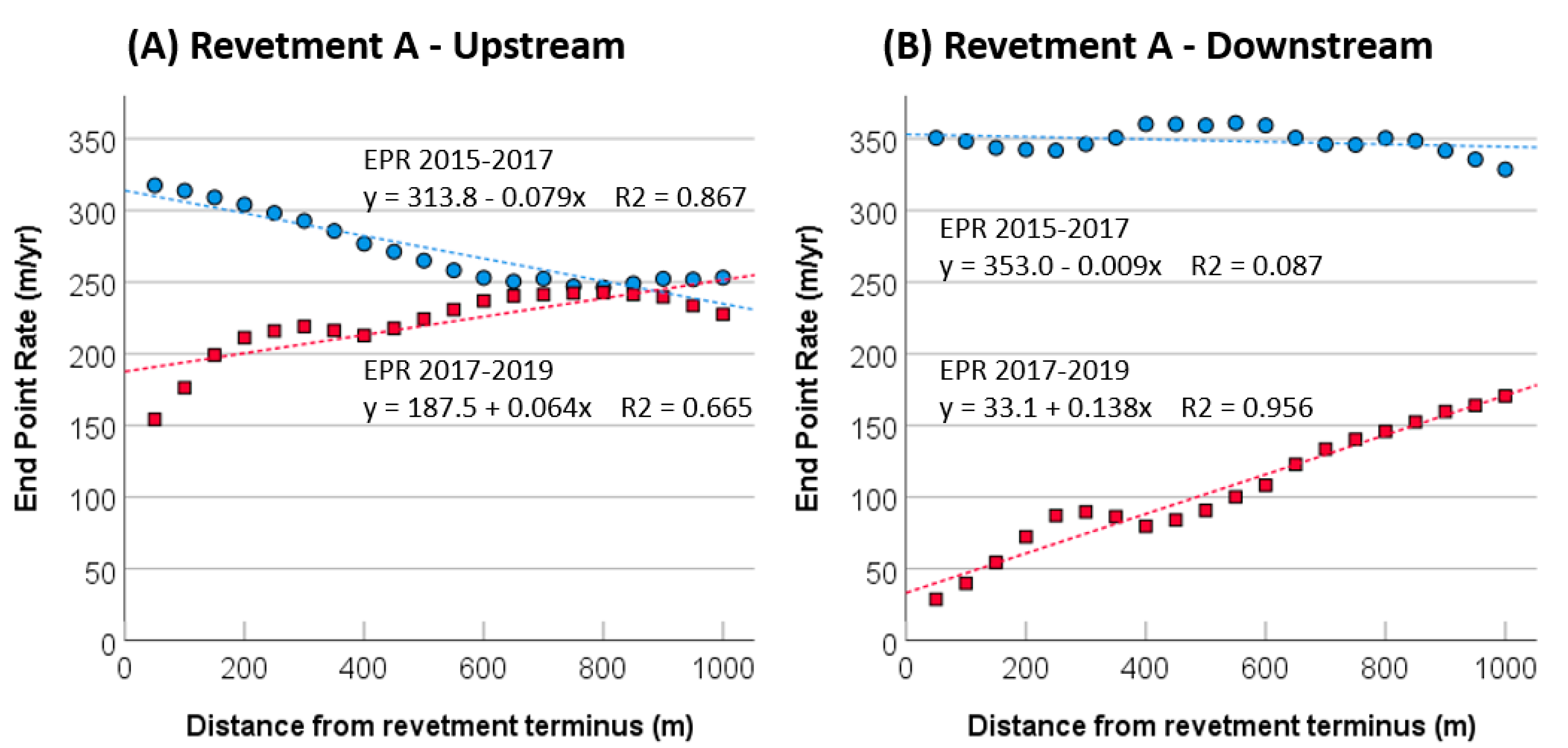
Q3. For each of the two new revetments, how have erosion rates changed for areas at the terminal ends of the revetments for the periods after the revetments were completed?

Using difEPR with the same before/after temporal scheme described above (Table 6), four sets of 20 transects each set representing 1 km of shoreline upstream and downstream of Revetments A and B were subset for analysis. Summary statistics characterize EPR and difEPR, and t-tests were applied separately to test for differences in EPR and difEPR comparing upstream versus downstream locations. Based on prior research identifying downdrift heightened erosion effects of coastal defenses, we hypothesize that EPR_After will be larger for downstream sites compared to upstream sites.

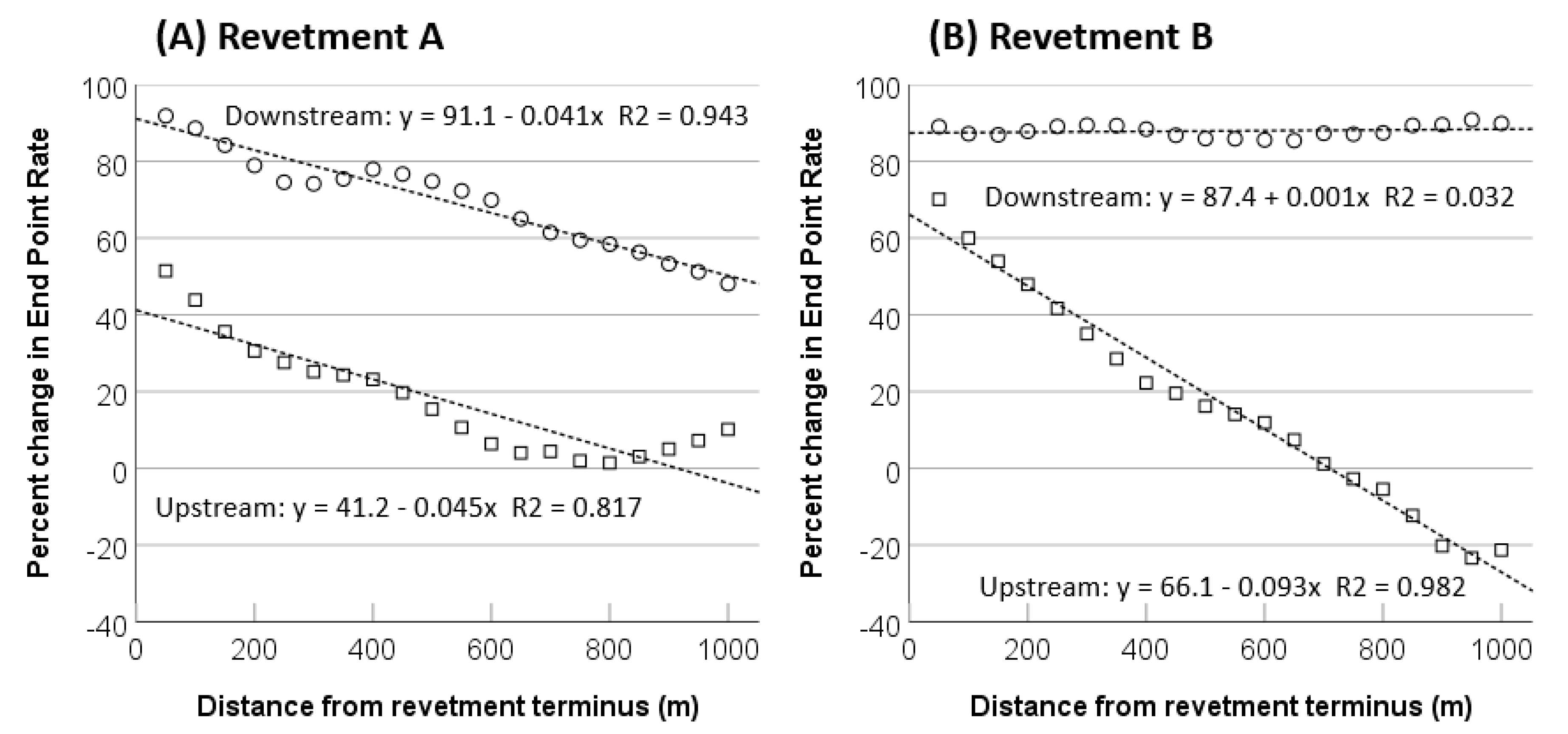
To assess the relative magnitudes of EPR change as percent change in EPR, %difEPR was defined as follows:

%difERP = ((EPR_Before − EPR_After)/(EPR_Before)) × 100

(4)

EPR_Before and EPR_After were defined using the same temporal schemes as earlier.

Graphical plots are used to visually reveal patterns EPR and %difEPR at the individual transect level where the x-axis represents upstream or downstream distance from revetment terminus points, and the y-axis represents EPR or %difEPR.

Q4. Are there differences in how households perceive erosion risk depending on if they are located in regions that are protected or unprotected by a new revetment?

Cross-tabulations were applied to responses for the four survey questions and interpreted. A general expectation was that revetment installation would be perceived positively by respondents in all regions such that no explicit hypotheses are specified, however it is possible that perceptions may vary by respondent location depending on potentially varying rates of erosion and relative location of respondents with respect to the new embankment. Following an inductive approach, we are curious to discern potential differences.

3. Results

3.1. Rates of Shoreline Change

Figure 6 reveals patterns of shoreline erosion for the 2011–2019 period showing visually that the North region (Kamalnagar) experienced higher erosion rates than the South region (Ramgati).

Table 7. Shoreline erosion by region, End Point Rate in m/y.

Change Period	North Region (n = 292)		South Region (n = 341)		t-Test Significance
	Mean EPR	Std. EPR	Mean EPR	Std. EPR
2011–2019	217.1	97.5	89.2	51.3	<0.001
2011–2012	310.6	128.3	123.9	111.3	<0.001
2012–2013	235.4	125.5	104.0	92.9	<0.001
2013–2014	284.4	149.6	133.5	100.9	<0.001
2014–2015	259.6	145.2	87.1	71.8	<0.001
2015–2016	227.3	107.2	82.5	91.4	<0.001
2016–2017	196.5	111.3	77.9	84.7	<0.001
2017–2018	135.6	80.0	63.1	65.8	<0.001
2018–2019	103.7	70.7	45.6	61.1	<0.001

provides quantitative information and associated t-test results that reveal a significantly higher erosion rate in the North region. All transects are included here for both protected and unprotected sites. Positive values for EPR indicate erosion. No transects experienced accretion over the 2011–2019 period, although a small number of transects had negative values of EPR for the various annual resolution results indicating accretion. All positive accretion values had a low magnitude that can be discounted due to spatial uncertainty.

For the full 2011–2019 period (first row in Table 7), the mean EPR for North was 127.9 m/y greater than for the South. Differences in mean EPR varied for individual one-year change periods but were significantly different for all cases. For the change periods of 2013–2014 and later, erosion experienced a downward trend for both regions.

3.2. Effects of Revetment for Protected Shoreline

Results provide evidence that, as expected, the revetments effectively halted erosion (

Table 8. End Point Rate (EPR) in m/y after revetment installation (positive indicates erosion).

	Revetment A EPR 2017–2019	Revetment B EPR 2015–2019
Number of transects intersecting revetment	19	64
Minimum EPR	−2.32	0.51
Maximum EPR	24.23	9.67
Mean EPR	5.51	4.01
Std. Error of EPR	1.62	0.30
Std. Deviation of EPR	7.08	2.44
Mean difference from EPR = 10	−4.49	−5.99
t-test sig. of mean difference from EPR = 10	p = 0.006	p < 0.001
95% conf. of mean difference from EPR = 10	(−7.90, −1.08)	(−6.60, −5.38)

) with mean EPR values of 5.51 m/y and 4.01 m/y for Revetments A and B, respectively, during the period after revetment installation. For comparison, note the much higher EPR values in Table 7 for the entire study area. EPR values for shorelines fronting the revetments were essentially zero after revetment installation. Recall that spatial uncertainty makes it impossible for EPR to be exactly zero causing us to use a comparison rate of EPR = 10 m/y for one-sample t-tests. Test results showed that mean EPR values were significantly less than 10 m/y. Higher variability is present for Revetment A ranging from −2.32 to 24.23. For Revetment A, the spatial pattern of transect-specific EPRs (not shown) revealed lower EPR for transects located at the revetment center and a consistent pattern of increasing EPR with distance away from the center. This is likely due to construction initiation in 2017 at the revetment’s center and progressing outward within the completion period.

Results for magnitudes of EPR change reported as difEPR show expected large changes (

Table 9. Change in EPR (difEPR) m/y for periods before/after revetment installation, m/y.

	Revetment A difEPR	Revetment B difEPR
Number of transects intersecting revetment	19	64
Minimum difEPR	297.74	153.40
Maximum difEPR	360.02	127.83
Mean difEPR	333.65	201.45
Std. Error of mean difEPR	3.97	2.43
Std. Deviation of difEPR	17.32	20.34
95% conf. of mean difEPR	(325.30, 342.00)	(148.32,158.49)

). Transects for Revetment A had a mean lower EPR of 333.65 m/y for the 2017–2019 after period compared to the 2015–2017 before period. Transects for Revetment B had a mean lower EPR of 201.45 m/y for the 2015–2019 after period compared to the 2011–2019 before period. It is tempting to make comparisons between Revetments A and B. This would be incorrect due to the different periods and because, in general, EPR in the North region of Kamalnagar Upazila where Revetment A is located is significantly higher than for the South region of Ramgati Upazila where Revetment B is located. In terms of percent reduction, both revetments essentially had a 100% reduction of erosion (calculated but not shown).

3.3. Effects of Revetment of Proximal Unprotected Shoreline

Table 10. End Point Rate (EPR, m/y) difference of means by upstream/downstream position and period.

	Upstream (n = 20)		Downstream (n = 20)
Revetment and Period	Mean EPR	Std. Error EPR	Mean EPR	Std. Error EPR	t-Test p-Value
Revetment A: 2015–2017	272.3	5.6	348.5	1.9	<0.001
Revetment A: 2017–2019	221.1	5.2	105.4	9.3	<0.001
Revetment B: 2011–2015	142.7	3.1	217.7	0.5	<0.001
Revetment B: 2015–2019	114.5	6.5	26.3	0.8	<0.001

compares mean EPR by upstream/downstream position for the before/after periods. All t-tests results indicate statistically significant differences of means. For both revetments, mean EPR was greater for the 20 downstream transects during the before periods (A: 2015–2017, B: 2011–2015). Mean EPR decreased substantially for both upstream and downstream transects, but notably and for both revetments, mean EPR switched to be greater for the 20 upstream transects compared to the downstream transects during the after periods. This latter result is counter to our hypothesis expecting EPR to be greater for the downstream transects due to downdrift effects of coastal defenses.

Table 11. End Point Rate change: difEPR and %difEPR difference of means by upstream/downstream position.

	Upstream (n = 20)		Downstream (n = 20)
Revetment	Mean	Std. Error	Mean	Std. Error	t-Test p-Value
Revetment A: difEPR	51.2 m/y	10.5 m/y	243.1 m/y	45.9 m/y	<0.001
Revetment A: %difEPR	17.5%	3.3%	69.6%	2.8%	<0.001
Revetment B: difEPR	28.2 m/y	9.4 m/y	191.3 m/y	0.8 m/y	<0.001
Revetment B: %difEPR	17.2%	6.2%	87.9%	0.3%	<0.001

compares difEPR and %difERP for upstream/downstream transects. Raw erosion rates (difEPR) were reduced substantially for both revetments for both upstream and downstream positions. For percent change (%difEPR), results show much greater erosion reduction for downstream transects for both revetments. Percent reductions were 69.6% and 87.9% for downstream transects which are much higher than the 17.5% and 17.2% reductions for upstream transects.

Graphical plots reveal patterns of EPR change. For Revetment A’s upstream transects, EPR during the before period (2015–2017) is at a maximum closest to the revetment terminus and exhibits a declining trend with distance (Figure 7a). This pattern reverses for the after period (2017–2019) where EPR is at a minimum for transects closest to the terminus and exhibits an increasing trend with distance.

For Revetment A’s downstream transects, EPR during the before period shows no trend (Figure 7b). However, for the after period and similar to upstream transects though at a lower magnitude, EPR is at a minimum for transects closest to the terminus and exhibits an increasing trend with distance.

For both upstream and downstream transects of Revetment A, the percent change in EPR shows a maximum percent erosion reduction for transects closest to revetment ends and a declining trend with distance (Figure 8a). Percent reductions were substantially higher for downstream transects.

For Revetment B’s upstream transects, EPR during the before period (2011–2015) is at a maximum closest to the revetment terminus and exhibits a declining trend (Figure 9a). This pattern reverses for the after period (2015–2019) where EPR is at a minimum for transects closest to the terminus and exhibits an increasing trend, though it is notable that the after period EPR crosses over to become higher than the before period EPR at 750 m. The upstream trends for Revetment B are similar to that of Revetment A (Figure 7a), notwithstanding the crossover in EPR.

For Revetment B’s downstream transects, EPR during both the before and after periods shows no trend (Figure 9b). However, erosion was reduced substantially for these sites.

For Revetment B, percent change in EPR shows no trend with distance for downstream transects (Figure 8b), a pattern that differs from Revetment A’s declining trend (Figure 8a). However, there is a notable declining trend for upstream transects (Figure 8b), which is approximately twice the magnitude of the trend for Revetment A (Figure 8a). A notable difference is a transition at 750 m to negative values reflective of the crossover to slightly higher upstream erosion at transect from 750 to 1000 m after the installation of the revetment (see Figure 9a).

3.4. Household Perception of Revetment Protection

Respondents were overwhelming in expressing a positive desire for engineered revetment (

Table 12. Perception of need for revetment construction for local area and extended area.

A. How do you agree that, “an engineered concrete revetment should be constructed to protect the Meghna River shoreline of my union”?
	Region 1	Region 2	Region 3	All Regions
Agree	201	90	93	384
	100.0%	96.8%	98.9%	99.0%
Neutral	0	0	0	0
	0.0%	0.0%	0.0%	0.0%
Disagree	0	3	1	4
	0.0%	3.2%	1.1%	1.0%
Total	201	93	94	388
	100.0%	100.0%	100.0%	100.0%
B. How do you agree that, “an engineered concrete embankment should be constructed to protect the entire Meghna River shoreline of my union all the way to Chandpur approximately 100 km north of here”?
	Region 1	Region 2	Region 3	All Regions
Agree	193	90	90	373
	96.0%	95.7%	92.8%	95.1%
Neutral	8	1	7	16
	4.0%	1.1%	7.2%	4.1%
Disagree	0	3	0	3
	0.0%	3.2%	0.0%	0.8%
Total	201	94	97	392
	100.0%	100.0%	100.0%	100.0%

A). For All Regions, 99.0% agreed or strongly agreed that revetment should be constructed for their union’s shoreline. Note that Region 2 had a revetment presence at the time of the survey. Results were similar for the perception of desire for revetments to be constructed from the study area to Chandpur located approximately 100 km upstream.

When asked more generally if revetment construction is a positive thing, respondents were again overwhelmingly positive with a combined 96.9% of All Regions with little variation among the individual regions (

Table 13. General perception of revetment and perception of negative erosion impacts for proximal unprotected shorelines due to revetment.

A. How do you agree that, “I think the revetment construction in recent years near my area is a positive thing”?
	Region 1	Region 2	Region 3	All Regions
Agree	196	92	92	380
	97.5%	97.9%	94.8%	96.9%
Neutral	5	1	1	7
	2.5%	1.1%	1.0%	1.8%
Disagree	0	1	4	5
	0.0%	1.1%	4.1%	1.3%
Total	201	94	97	392
	100.0%	100.0%	100.0%	100.0%
B. How do you agree that, “I think the revetment acts to protect areas near the revetment but acts to make riverbank erosion worse for other areas that are not immediately protected by the embankment”?
	Region 1	Region 2	Region 3	All Regions
Agree	21	19	6	46
	75.0%	44.2%	35.3%	52.3%
Neutral	3	18	9	30
	10.7%	41.9%	52.9%	34.1%
Disagree	4	6	2	12
	14.3%	14.0%	11.8%	13.6%
Total	28	43	17	88
	100.0%	100.0%	100.0%	100.0%

A).

Perceptions were mixed to the question asking if the revetment makes erosion worse for areas not immediately near and protected by the revetment (Table 13B). Note that, unlike the prior survey question results, here households were subset to include the n = 88 that were within 1 km of the 2018 shoreline and those protected by the embankment (e.g., behind the embankment, Region 2) or within 1 km of the revetment’s terminal end either upstream (Region 1) or downstream (Region 3). This was done to focus on perceptions for households located most near the revetment for which respondents arguably have the most heightened perception of revetment effects. Strikingly, upstream household respondents (Region 1) had a strong majority perception (75.0%) that revetment acts to make erosion worse. Downstream respondents agreed at the lowest level (35.3%) that revetment worsens erosion with a majority expressing a neutral perception (52.9%). Low percentages across all regions disagree that the revetment makes erosion worse. Relatively higher percentages of respondents in Regions 2 and 3 had a neutral opinion, which is perhaps due to the newness of the revetment.

4. Discussion

This research investigated the problem of coastal erosion and the strategy of engineered shoreline protection as a mitigation tool to reduce erosion risk for economically challenged population in Bangladesh with high vulnerability. In doing so, we implemented a combination of geospatial and social science methods to answer research questions regarding rates and patterns of shoreline erosion, the mitigative effects of newly constructed revetments, and human perceptions of revetment desirability and efficacy. Key summarized results, interpretation, and discussion are presented below.

Two recently constructed revetments effectively halted erosion for the 1.5 km and 3.2 km of shoreline protected by Revetments A and B. This is an expected result; however, it is notable that magnitudes of change (lowered erosion) immediately before and after revetment installation were 333.65 m/y and 201.45 m/y. Clearly, vulnerable households protected by these revetments benefit from reduced erosion risk. Related research using the same social survey data estimates that 24 households lost their homes to erosion [17] from May 2018 to January 2019. All were located upstream of Ramgati’s Revetment B. In the absence of Revetment B, many households currently protected by the revetment might have been lost to erosion. Along with the clear household benefits of revetment protection for households located directly behind the revetment, revetment failure is a concern that warrants monitoring and remediation. News reports state that the northern revetment (Revetment A) has already experienced damage threatening this region, which has extreme erosion rates.

“The Meghna river protection dam under Kamalnagar Upazila of the district [Revetment A] is now under threat due to its bank erosion, spreading panic among villagers. Locals said it might disappear in the river as some 200 m of the dam have already been washed away due to strong current for the last two days. They alleged that the poorly-built dam collapses frequently as there were widespread irregularities in its construction—from the beginning to the end” [37].

Results showed erosion to have decreased substantially for upstream and downstream sites within 1 km of the ends of Revetments A and B.

Table 14. Summarized results of erosion patterns for transects located within 1 km of revetment terminal ends (D = downstream, U = Upstream).

	(1)	(2)	(3)	(4)	(5)	(6)	(7)	(8)	(9)	(10)
Revet-ment	Mean EPR Before	Mean EPR After	Mean EPR Change	Mean % EPR Change	Upstrm EPR Trend Before	Upstrm EPR Trend After	Downstrm EPRTrend Before	Downstrm EPR Trend After	Upstrm % EPR Change Trend Before	Downstrm % EPR Change Trend After
A	D > U	U > D	D > U	D > U	↘	↗	→	↗	↘	↘
B	D > U	U > D	D > U	D > U	↘	↗	→	→	↘	→

summarizes differences and trends for the upstream and downstream locations.

Interestingly and for both revetments, downstream sites initially had higher erosion than upstream sites (Col. 1). After revetment installation, upstream sites had higher erosion (Col. 2). Downstream sites experienced the greatest raw and percentage change reduction in erosion (Cols. 3–4).

The finding that downstream sites experienced lower erosion than upstream sites after revetment installation runs counter to the hypothesis expecting downdrift effects to result in higher erosion for downstream sites as has been found in other research [28,29,30], although we note that both sites experience lower erosion overall. Much of the prior research has been for sandy ocean beaches with prevailing longshore currents driving the downdrift effect. While our estuarine site experiences prevailing currents in the downstream direction, tidal influences operating in the reverse direction from the Bay of Bengal may be acting to attenuate downdrift effects. Further, we wonder if the higher downstream current velocity during the monsoon period [61] is more attenuated for downstream sites such that upstream sites have relatively higher exposure to hydrodynamic energy and causes these relative differences in erosion patterns. The fact that the North region has higher erosion than the South region is a suggestive pattern where the seasonal monsoon pulse of erosive energy driven by fluvial discharge from the GBM basin is greater with increasing distance from the Bay of Bengal. Further geophysical and processed-based analyses including integrating analysis of wind, wave, and bathymetry data are required to better explain this pattern.

Upstream sites for both revetments initially had a downward spatial trend; e.g., higher erosion closer to the revetment that decreases with distance (Col. 5). This trend switched to an upward trend (Col. 6) indicating lower erosion closer to the revetment that increases with distance. Given that upstream sites experienced lower erosion overall after revetment installation, upstream households located closer to the revetment especially benefitted from the overall reduced erosion. Downstream sites showed no spatial trend before the revetments (Col. 7) while experiencing greater raw and percent erosion reduction (Cols. 3 and 4) compared to upstream sites.

Downstream sites of Revetment A (and associated near-shoreline households) experienced the greatest benefits of all sites from reduced erosion after new revetment. They had the greatest mean and percent erosion reduction. Further, the upward spatial trend after the revetment (Col. 8) reveals that downstream households located closer to the revetment benefitted the most from reduced erosion.

After revetment installation, the spatial patterns for all sites except those downstream of Revetment B (Cols. 6 and 8) exhibited an increasing trend of erosion rates with distance from terminal ends suggesting benefits of revetments for these most proximal sites. For the two upstream sites (transects upstream of Revetments and B), this was a trend reversal (see Cols. 5 and 6) from the period before revetment installation where sites closest to terminal ends had highest erosion rates and declining rates with increasing distance from terminal ends.

Results for near-embankment patterns and distance effects are described that warrant further investigation of the process dynamics. Possible explanations include localized offshore bar formation that alters currents differentially depending on location.

Survey results focusing solely on Revetment B in Ramgati showed that virtually all households desired revetment protection regardless of status—protected, upstream, or downstream. However, there were notable differences in perceptions of the revetment’s effects depending on household location. Notably, upstream respondents located within 1 km of the shoreline and 1 km of the revetment terminus strongly perceived that the revetment acted to make erosion worse. This result is interesting because these sites experienced lower erosion rates after revetment installation and within a context where the general trend of erosion rates has declined in the recent years before the survey, as did the entire study area. However, when viewed comparatively, nearby revetment-protected sites experienced a halt of erosion due to new revetment. Further and prior to the revetment, sites downstream from the revetment had comparatively higher erosion rates. This pattern reversed after the revetment such that upstream sites had higher erosion. Thus, and in a relative sense, upstream households became worse off concerning erosion rates compared to downstream households even though, in an absolute sense, erosion rates were reduced for both upstream and downstream sites.

Conversely, downstream respondents had the lowest perception that the revetment acted to make erosion worse. It is intriguing to question if this relative difference caused downstream respondents to perceive their erosion situation to have improved due to the perception of downstream relative erosion in addition to the absolute reduction of erosion rates for their shoreline. However, it is notable that a substantial percent of downstream respondents still perceived that the revetment acts to make erosion worse. A caveat is that the data do not permit direct interpretation of respondent perceptions relative to the other sites (e.g., protected vs. upstream vs. downstream). It is possible and even likely that respondents may have perceptions of erosion rates for other sites that inform responses.

5. Conclusions

The study describes research integrating remote sensing and social science data to answer questions regarding space–time patterns of coastal erosion in a region at high risk and the efficiacy/efficiency and human perception of revetments as a coastal protection strategy. Research that links remote sensing analysis of shoreline change with social data describing population at effected sites is uncommon. This work is innovative because, in addition to the empirial analysis of shoreline change, it analyzes the perceptions of human population located in close proximity to newly constructed embankment which alters erosion patterns. The use of high-resolution Planet Lab imagery with spatial analysis methods was shown to be an effective methodology revealing significant space–time erosion patterns. Revetments were found to halt erosion effectively and to be associated with upstream and downstream effects of nearby unprotected shorelines. Local population overwhelmingly have positive views of the revetment strategy and expressed a desire for continuous “wall-to-wall” protection for the eastern bank of the Lower Meghna estuary. Constructing continuous revetment protection would require a tremendous investment of resources, which makes this prospect unlikely in a developing country like Bangladesh and without significant political will, financial commitment, and international aid. Further, large-scale revetment protection would significantly alter the naturally occurring geophysical processes of this region of the Bangladesh delta, potentially in unforseen ways. While it is true that major protective infrastructure has been constructed throughout other parts of the Bangladesh coast, a new initiative would require a thorough scientific analysis of the costs and benefits. Future work should continue to monitor erosion patterns and revetment effects. It should further evaluate the social drivers (e.g., age, previous experience, education, income, employment sector, gender, etc.) of human perceptions of erosion risk and revetment as a mitigative strategy. The vast majority of shoreline proximal population in the study region will remain unprotected by coastal defenses for the foreseeable future and will continue to engage in livelihood strategies involving the evaluation of risk informing household behaviors, including the potential of erosion-induced migration. Future household disruption, response, and resilience will likely vary depending on the variation in household location/risk coupled with differentials in human, social, economic, and technological capital.

References

1. Sahoo, B.; Bhaskaran, P.K. Multi-hazard risk assessment of coastal vulnerability from tropical cyclones—A GIS based approach for the Odisha coast. J. Environ. Manag. 2018, 206, 1166–1178. [Google Scholar] [CrossRef] [PubMed]
2. Klein, R.J.T.; Nicholls, R.J.; Thomalla, F. Resilience to natural hazards: How useful is this concept? Environ. Hazards 2003, 5, 35–45. [Google Scholar] [CrossRef]
3. Passeri, D.L.; Hagen, S.C.; Medeiros, S.C.; Bilskie, M.V.; Alizad, K.; Wang, D. The dynamic effects of sea level rise on low-gradient coastal landscapes: A review. Earth’s Future 2015, 3, 159–181. [Google Scholar] [CrossRef]
4. Woodroffe, C.D.; Nicholls, R.J.; Saito, Y.; Chen, Z.; Goodbred, S.L. Landscape Variability and the Response of Asian Megadeltas to Environmental Change. In Global Change and Integrated Coastal Management: The Asia-Pacific Region; Harvey, N., Ed.; Coastal Systems and Continental Margins; Springer: Dordrecht, The Netherlands, 2006; pp. 277–314. ISBN 978-1-4020-3628-6. [Google Scholar]
5. IPCC WGI. Climate Change 2001, Scientific Basis; Cambridge University Press: Cambridge, UK, 2001; p. 881. [Google Scholar]
6. Choudhury, N.Y.; Paul, A.; Paul, B.K. Impact of costal embankment on the flash flood in Bangladesh: A case study. Appl. Geogr. 2004, 24, 241–258. [Google Scholar] [CrossRef]
7. Koh, C.-H.; De Jonge, V.N. Stopping the disastrous embankments of coastal wetlands by implementing effective management principles: Yellow Sea and Korea compared to the European Wadden Sea. Ocean Coast. Manag. 2014, 102, 604–621. [Google Scholar] [CrossRef]
8. Vos, K.; Splinter, K.D.; Harley, M.D.; Simmons, J.A.; Turner, I.L. CoastSat: A Google Earth Engine-enabled Python toolkit to extract shorelines from publicly available satellite imagery. Environ. Model. Softw. 2019, 122, 104528. [Google Scholar] [CrossRef]
9. Luijendijk, A.; Hagenaars, G.; Ranasinghe, R.; Baart, F.; Donchyts, G.; Aarninkhof, S. The State of the World’s Beaches. Sci. Rep. 2018, 8, 6641. [Google Scholar] [CrossRef]
10. Thieler, E.R.; Himmelstoss, E.A.; Zichichi, J.L.; Ergul, A. The Digital Shoreline Analysis System (DSAS) Version 4.0—An ArcGIS Extension for Calculating Shoreline Change; Open-File Report 2008-1278; U.S. Geological Survey: Reston, VA, USA, 2009.
11. Chowdhury, M.R.; Ward, N. Hydro-meteorological variability in the greater Ganges–Brahmaputra–Meghna basins. Int. J. Climatol. 2004, 24, 1495–1508. [Google Scholar] [CrossRef]
12. Islam, A.S.; Haque, A.; Bala, S.K. Hydrologic characteristics of floods in Ganges–Brahmaputra–Meghna (GBM) delta. Nat. Hazards 2010, 54, 797–811. [Google Scholar] [CrossRef]
13. Woodroffe, C.D.; Saito, Y. 3.05—River-Dominated Coasts. In Treatise on Estuarine and Coastal Science; Wolanski, E., McLusky, D., Eds.; Academic Press: Waltham, MA, USA, 2011; pp. 117–135. ISBN 978-0-08-087885-0. [Google Scholar]
14. Coleman, J.M. Brahmaputra river: Channel processes and sedimentation. Sediment. Geol. 1969, 3, 129–239. [Google Scholar] [CrossRef]
15. Brammer, H. Bangladesh’s dynamic coastal regions and sea-level rise. Clim. Risk Manag. 2014, 1, 51–62. [Google Scholar] [CrossRef] [Green Version]
16. Ahmed, A.; Drake, F.; Nawaz, R.; Woulds, C. Where is the coast? Monitoring coastal land dynamics in Bangladesh: An integrated management approach using GIS and remote sensing techniques. Ocean Coast. Manag. 2018, 151, 10–24. [Google Scholar] [CrossRef]
17. Crawford, T.; Rahman, M.; Paul, B.K.; Curtis, S. Coupled Adaptive Cycles of Shoreline Change and Households in Deltaic Bangladesh: Analysis of a 30-Year Shoreline Change Record and Recent Population Impacts. Ann. AAG 2020, in press. [Google Scholar]
18. Hossain, S.; Dearing, J.A.; Rahman, M.M.; Salehin, M. Recent changes in ecosystem services and human well-being in the Bangladesh coastal zone. Reg. Environ. Chang. 2016, 16, 429–443. [Google Scholar] [CrossRef] [Green Version]
19. Poncelet, A.; Gemenne, F.; Martiniello, M.; Bousetta, H. A Country Made for Disasters: Environmental Vulnerability and Forced Migration in Bangladesh. In Environment, Forced Migration and Social Vulnerability; Afifi, T., Jäger, J., Eds.; Springer: Berlin/Heidelberg, Germany, 2010; pp. 211–222. ISBN 978-3-642-12416-7. [Google Scholar]
20. Rahman, R.; Salehin, M. Flood Risks and Reduction Approaches in Bangladesh. In Disaster Risk Reduction Approaches in Bangladesh; Shaw, R., Mallick, F., Islam, A., Eds.; Disaster Risk Reduction; Springer: Tokyo, Japan, 2013; pp. 65–90. ISBN 978-4-431-54252-0. [Google Scholar]
21. Paul, B.; Rashid, H. Climatic Hazards in Coastal Bangladesh: Non-Structural and Structural Solutions; Butterworth-Heinemann: Oxford, UK, 2016; ISBN 978-0-12-804612-8. [Google Scholar]
22. Nicholls, R.J.; Hutton, C.W.; Lázár, A.N.; Allan, A.; Adger, W.N.; Adams, H.; Wolf, J.; Rahman, M.; Salehin, M. Integrated assessment of social and environmental sustainability dynamics in the Ganges-Brahmaputra-Meghna delta, Bangladesh. Estuar. Coast. Shelf Sci. 2016, 183, 370–381. [Google Scholar] [CrossRef] [Green Version]
23. Sarwar, G.M.; Woodroffe, C.D. Rates of shoreline change along the coast of Bangladesh. J. Coast. Conserv. 2013, 17, 515–526. [Google Scholar] [CrossRef] [Green Version]
24. Griggs, G.B.; Tait, J.F. The Effects of Coastal Protection Structures on Beaches Along Northern Monterey Bay, California. J. Coast. Res. 1988, 4, 93–111. [Google Scholar]
25. Hardaway, C.S.; Byrne, R. Shoreline Management in Chesapeake Bay; Special Report in Applied Marine Science and Ocean Engineering No. 356; Virginia Institute of Marine Science: Gloucester Point, VA, USA, 1999. [Google Scholar] [CrossRef]
26. Kraus, N.C.; McDougal, W.G. The Effects of Seawalls on the Beach: Part I, an Updated Literature Review. J. Coast. Res. 1996, 12, 691–701. [Google Scholar]
27. Basco, D.R. Seawall Impacts on Adjacent Beaches: Separating Fact from Fiction. J. Coast. Res. 2006, 2, 741–744. [Google Scholar]
28. Jayappa, K.S.; Kumar, G.T.V.; Subrahmanya, K.R. Influence of Coastal Structures on the Beaches of Southern Karnataka, India. J. Coast. Res. 2003, 19, 389–408. [Google Scholar]
29. Brown, S.; Barton, M.; Nicholls, R. Coastal retreat and/or advance adjacent to defences in England and Wales. J. Coast. Conserv. 2011, 15, 659–670. [Google Scholar] [CrossRef] [Green Version]
30. Brown, S.; Barton, M.E.; Nicholls, R.J. Shoreline response of eroding soft cliffs due to hard defences. Proc. Inst. Civ. Eng. Marit. Eng. 2014, 167, 3–14. [Google Scholar] [CrossRef] [Green Version]
31. Kaliraj, S.; Chandrasekar, N.; Ramachandran, K.K.; Srinivas, Y.; Saravanan, S. Coastal landuse and land cover change and transformations of Kanyakumari coast, India using remote sensing and GIS. Egypt. J. Remote Sens. Space Sci. 2017, 20, 169–185. [Google Scholar] [CrossRef]
32. Khan, N.I.; Islam, A. Quantification of erosion patterns in the Brahmaputra—Jamuna River using geographical information system and remote sensing techniques. Hydrol. Process. 2003, 17, 959–966. [Google Scholar] [CrossRef]
33. Baki, A.B.M.; Gan, T.Y. Riverbank migration and island dynamics of the braided Jamuna River of the Ganges–Brahmaputra basin using multi-temporal Landsat images. Quat. Int. 2012, 263, 148–161. [Google Scholar] [CrossRef]
34. Rahman, A.F.; Dragoni, D.; El-Masri, B. Response of the Sundarbans coastline to sea level rise and decreased sediment flow: A remote sensing assessment. Remote Sens. Environ. 2011, 115, 3121–3128. [Google Scholar] [CrossRef]
35. Ashraful Islam, M.; Mitra, D.; Dewan, A.; Akhter, S.H. Coastal multi-hazard vulnerability assessment along the Ganges deltaic coast of Bangladesh–A geospatial approach. Ocean Coast. Manag. 2016, 127, 1–15. [Google Scholar] [CrossRef]
36. Salauddin, M.; Hossain, K.T.; Tanim, I.A.; Kabir, M.A.; Saddam, M.H. Modeling Spatio-Temporal Shoreline Shifting of a Coastal Island in Bangladesh Using Geospatial Techniques and DSAS Extension. Ann. Valahia Univ. Targoviste Geogr. Ser. 2018, 18, 1–13. [Google Scholar] [CrossRef] [Green Version]
37. Dada, O.A.; Li, G.; Qiao, L.; Ding, D.; Ma, Y.; Xu, J. Seasonal shoreline behaviours along the arcuate Niger Delta coast: Complex interaction between fluvial and marine processes. Cont. Shelf Res. 2016, 122, 51–67. [Google Scholar] [CrossRef]
38. Ghoneim, E.; Mashaly, J.; Gamble, D.; Halls, J.; AbuBakr, M. Nile Delta exhibited a spatial reversal in the rates of shoreline retreat on the Rosetta promontory comparing pre- and post-beach protection. Geomorphology 2015, 228, 1–14. [Google Scholar] [CrossRef]
39. Esmail, M.; Mahmod, W.E.; Fath, H. Assessment and prediction of shoreline change using multi-temporal satellite images and statistics: Case study of Damietta coast, Egypt. Appl. Ocean Res. 2019, 82, 274–282. [Google Scholar] [CrossRef]
40. Zhang, X.; Yang, Z.; Zhang, Y.; Ji, Y.; Wang, H.; Lv, K.; Lu, Z. Spatial and temporal shoreline changes of the southern Yellow River (Huanghe) Delta in 1976–2016. Mar. Geol. 2018, 395, 188–197. [Google Scholar] [CrossRef]
41. Qiao, G.; Mi, H.; Wang, W.; Tong, X.; Li, Z.; Li, T.; Liu, S.; Hong, Y. 55-year (1960–2015) spatiotemporal shoreline change analysis using historical DISP and Landsat time series data in Shanghai. Int. J. Appl. Earth Obs. Geoinf. 2018, 68, 238–251. [Google Scholar] [CrossRef]
42. Jana, A.; Biswas, A.; Maiti, S.; Bhattacharya, A.K. Shoreline changes in response to sea level rise along Digha Coast, Eastern India: An analytical approach of remote sensing, GIS and statistical techniques. J. Coast. Conserv. 2014, 18, 145–155. [Google Scholar] [CrossRef]
43. Natesan, U.; Parthasarathy, A.; Vishnunath, R.; Kumar, G.E.J.; Ferrer, V.A. Monitoring Longterm Shoreline Changes along Tamil Nadu, India Using Geospatial Techniques. Aquat. Procedia 2015, 4, 325–332. [Google Scholar] [CrossRef]
44. Rani, M.; Rehman, S.; Sajjad, H.; Chaudhary, B.S.; Sharma, J.; Bhardwaj, S.; Kumar, P. Assessing coastal landscape vulnerability using geospatial techniques along Vizianagaram–Srikakulam coast of Andhra Pradesh, India. Nat. Hazards 2018, 94, 711–725. [Google Scholar] [CrossRef]
45. Baral, R.; Pradhan, S.; Samal, R.N.; Mishra, S.K. Shoreline Change Analysis at Chilika Lagoon Coast, India Using Digital Shoreline Analysis System. J. Indian Soc. Remote Sens. 2018, 46, 1637–1644. [Google Scholar] [CrossRef]
46. Jayanthi, M.; Thirumurthy, S.; Samynathan, M.; Duraisamy, M.; Muralidhar, M.; Ashokkumar, J.; Vijayan, K.K. Shoreline change and potential sea level rise impacts in a climate hazardous location in southeast coast of India. Environ. Monit. Assess. 2017, 190, 51. [Google Scholar] [CrossRef]
47. Stevens, F.R.; Gaughan, A.E.; Linard, C.; Tatem, A.J. Disaggregating Census Data for Population Mapping Using Random Forests with Remotely-Sensed and Ancillary Data. PLoS ONE 2015, 10, e0107042. [Google Scholar] [CrossRef] [PubMed] [Green Version]
48. Planet Team. Planet Application Program Interface. In Space for Life on Earth; San Francisco, CA, USA, 2017; Available online: https://www.planet.com (accessed on 10 August 2019).
49. Maglione, P.; Parente, C.; Vallario, A. Coastline extraction using high resolution WorldView-2 satellite imagery. Eur. J. Remote Sens. 2014, 47, 685–699. [Google Scholar] [CrossRef]
50. Du, Z.; Li, W.; Zhou, D.; Tian, L.; Ling, F.; Wang, H.; Gui, Y.; Sun, B. Analysis of Landsat-8 OLI imagery for land surface water mapping. Remote Sens. Lett. 2014, 5, 672–681. [Google Scholar] [CrossRef]
51. Dai, C.; Howat, I.M.; Larour, E.; Husby, E. Coastline extraction from repeat high resolution satellite imagery. Remote Sens. Environ. 2019, 229, 260–270. [Google Scholar] [CrossRef]
52. McFeeters, S.K. The use of the Normalized Difference Water Index (NDWI) in the delineation of open water features. Int. J. Remote Sens. 1996, 17, 1425–1432. [Google Scholar] [CrossRef]
53. Hapke, C.J.; Himmelstoss, E.A.; Kratzman, M.G.; List, J.H.; Thieler, E.R. National Assessment of Shoreline Change: Historical Shoreline Changes along the New England and Mid-Atlantic Coasts; U.S. Geological Survey Open-File Report 2010-1118; USGS: Reston, VA, USA, 2010.
54. Mullick, R.A.; Islam, K.M.A.; Tanim, A.H. Shoreline change assessment using geospatial tools: A study on the Ganges deltaic coast of Bangladesh. Earth Sci. Inform. 2020, 13, 299–316. [Google Scholar] [CrossRef]
55. Nassar, K.; Mahmod, W.E.; Fath, H.; Masria, A.; Nadaoka, K.; Negm, A. Shoreline change detection using DSAS technique: Case of North Sinai coast, Egypt. Mar. Georesour. Geotechnol. 2019, 37, 81–95. [Google Scholar] [CrossRef]
56. Jana, S. Micro-level coastal vulnerability assessment in relation to post-Aila landscape alteration at the fragile coastal stretch of the Sagar Island, India. Reg. Stud. Mar. Sci. 2020, 33, 100908. [Google Scholar] [CrossRef]
57. Environmental System Research Institute How Grouping Analysis Works. Available online: https://pro.arcgis.com/en/pro-app/tool-reference/spatial-statistics/how-grouping-analysis-works.htm (accessed on 19 December 2019).
58. National Research Council; Division of Behavioral and Social Sciences and Education; Board on Environmental Change and Society; Committee on the Human Dimensions of Global Change. People and Pixels: Linking Remote Sensing and Social Science; National Academies Press: Washington, DC, USA, 1998; ISBN 978-0-309-06408-8. [Google Scholar]
59. Kugler, T.A.; Grace, K.; Wrathall, D.J.; De Sherbinin, A.; Van Riper, D.; Aubrecht, C.; Comer, D.; Adamo, S.B.; Cervone, G.; Engstrom, R.; et al. People and Pixels 20 years later: The current data landscape and research trends blending population and environmental data. Popul. Environ. 2019, 41, 209–234. [Google Scholar] [CrossRef]
60. Liverman, D.M.; Cuesta, R.M.R. Human interactions with the Earth system: People and pixels revisited. Earth Surf. Process. Landf. 2008, 33, 1458–1471. [Google Scholar] [CrossRef]
61. Alam, R.; Islam, S.; Hasib, M.R.; Khan, Z.H. Characteristics of Hydrodynamic Processes in the Meghna Estuary due to Dynamic Whirl Action. IOSR J. Eng. 2014, 4, 39–50. [Google Scholar] [CrossRef]
Figure 1. Revetments in Ramgati Upazila: (a,b) at Char Alexander, constructed 2015–2017; (c,d) at Ramgati Ghat, construction started in 2018 and ongoing at time of photos taken in January 2018 (photos by T. Crawford).
Remotesensing 12 03108 g001
Figure 2. New revetments constructed in Lakshmipur district: (A) Revetment A in Kamalnagar Upazila, (B) Revetment B in Ramgati Upazila, (C) Revetment C in Ramgati Upazila.
Remotesensing 12 03108 g002
Figure 3. Study area—shoreline of the eastern bank of the Lower Meghna river/estuary in Kamalnagar and Ramgati Upazilas of Lakshmipur District, Bangladesh.
Remotesensing 12 03108 g003
Figure 4. Example of transects at 50 m increments used for Digital Shoreline Analysis System (DSAS) shoreline change analysis; Normalized Difference Water Index (NDWI) from a 6 January 2019 PlanetScope image (3.7 m pixel) [48] in background; black indicates water; white shoreline strip is Revetment B in Ramgati Upazila; green line is 2011 shoreline; red line is 2019 shoreline.
Remotesensing 12 03108 g004
Figure 5. Sampled household locations by region in Ramgati Upazila; Region 2 is protected by a revetment; household location confidentiality was preserved by randomly shifting ±50 m in the x and y directions along with the choice of map scale and point symbol size; background image is a PlanetScope (3.7 m pixel) false color composite dated 6 January 2019 [48].
Remotesensing 12 03108 g005
Figure 6. Shoreline change rate map—End Point Rate, positive indicates erosion.
Remotesensing 12 03108 g006
Figure 7. Revetment A End Point Rate: (A) upstream, (B) downstream; circles = EPR for 2015–2017, squares = EPR for 2017–2019; linear regression trend lines shown.
Remotesensing 12 03108 g007
Figure 8. Percent change in End Point Rate: (A) Revetment A, (B) Revetment B; squares = upstream, circles = downstream; linear regression trend lines shown.
Remotesensing 12 03108 g008
Figure 9. Revetment B End Point Rate: (A) upstream, (B) downstream; circles = EPR for 2011–2015, squares = EPR for 2015–2019; linear regression trend line shown.
Remotesensing 12 03108 g009