Article

LS-SSDD-v1.0: A Deep Learning Dataset Dedicated to Small Ship Detection from Large-Scale Sentinel-1 SAR Images

1
School of Information and Communication Engineering, University of Electronic Science and Technology of China, Chengdu 611731, China
2
Aerospace Information Research Institute, Chinese Academy of Sciences, Beijing 100194, China
3
Department of Electronic and Information Engineering, Naval Aeronautical University, Yantai 264000, China
4
School of Electronic Information and Electrical Engineering, Shanghai Jiao Tong University, Shanghai 200240, China
*
Author to whom correspondence should be addressed.
Remote Sens. 2020, 12(18), 2997; https://doi.org/10.3390/rs12182997
Submission received: 14 August 2020 / Revised: 6 September 2020 / Accepted: 11 September 2020 / Published: 15 September 2020

Abstract

:
Ship detection in synthetic aperture radar (SAR) images is becoming a research hotspot. In recent years, as the rise of artificial intelligence, deep learning has almost dominated SAR ship detection community for its higher accuracy, faster speed, less human intervention, etc. However, today, there is still a lack of a reliable deep learning SAR ship detection dataset that can meet the practical migration application of ship detection in large-scene space-borne SAR images. Thus, to solve this problem, this paper releases a Large-Scale SAR Ship Detection Dataset-v1.0 (LS-SSDD-v1.0) from Sentinel-1, for small ship detection under large-scale backgrounds. LS-SSDD-v1.0 contains 15 large-scale SAR images whose ground truths are correctly labeled by SAR experts by drawing support from the Automatic Identification System (AIS) and Google Earth. To facilitate network training, the large-scale images are directly cut into 9000 sub-images without bells and whistles, providing convenience for subsequent detection result presentation in large-scale SAR images. Notably, LS-SSDD-v1.0 has five advantages: (1) large-scale backgrounds, (2) small ship detection, (3) abundant pure backgrounds, (4) fully automatic detection flow, and (5) numerous and standardized research baselines. Last but not least, combined with the advantage of abundant pure backgrounds, we also propose a Pure Background Hybrid Training mechanism (PBHT-mechanism) to suppress false alarms of land in large-scale SAR images. Experimental results of ablation study can verify the effectiveness of the PBHT-mechanism. LS-SSDD-v1.0 can inspire related scholars to make extensive research into SAR ship detection methods with engineering application value, which is conducive to the progress of SAR intelligent interpretation technology.

Graphical Abstract

1. Introduction

Synthetic aperture radar (SAR) is an active microwave imaging sensor whose all-day and all-weather working capacity give it an important place in marine exploration [1,2,3,4,5,6,7]. Since the United States launched the first SAR satellite, SAR has received much attention in marine remote sensing, e.g., geological exploration, topographic mapping, disaster forecast, traffic monitoring, etc. As a valuable ocean mission, SAR ship detection is playing a critical role in shipwreck rescue, fishery and traffic management, etc., so it is becoming a research hotspot [1,2,3,4,5,6,7,8,9,10,11,12,13,14,15,16,17,18,19,20,21,22,23,24,25,26,27,28,29,30,31,32,33,34,35,36,37,38,39,40,41,42,43,44,45,46,47,48,49,50,51,52,53,54,55,56,57,58,59,60,61,62,63,64,65,66,67,68,69,70].
So far, many traditional SAR ship detection methods have been proposed, e.g., global threshold-based [36,37,38], constant false alarm ratio (CFAR)-based [39,40,41], generalized likelihood ratio test (GLRT)-based [42,43,44], transformation domain-based [45,46,47], visual saliency-based [48,49,50], super-pixel segmentation-based [51,52,53], and auxiliary feature-based (e.g., ship-wake) [54,55,56], all of which obtained modest results in specific backgrounds, but these methods always extract ship features by hand-designed means, leading to complexity in computation, weakness in generalization, and trouble in manual feature extraction [1,4]. Moreover, as ship wakes do not exist all the time, and their features are not as obvious as ship targets, the research on the detection of ship wakes is not extensive [13].
With the rise of AI, deep learning [71] is providing much power for SAR ship detection. Based on our survey [8,10,11,12,13,14,15,16,17,18,19,20,21,22,23,24,25,26,27,28,29,30,31,32,33,34,35,61,62,70], deep learning has almost dominated the SAR ship detection community for its higher accuracy, faster speed, less human intervention, etc., so increasingly, scholars have made use of deep learning-based ship detection act in an important research direction. In the early stage, deep learning was applied in various parts of SAR ship detection, e.g., land masking [28], region of interest (ROI) extraction, and ship discrimination [28,72] (i.e., ship or background binary classification of a single chip). However, in the present stage, deep-learning-based SAR ship detection methods utilize an end-to-end mode to send SAR images into networks for detection and output detection results directly [13], without the support of auxiliary tools (e.g., traditional preprocessing tools, geo information, etc.) and without manual involvement, so the operation of sea–land segmentation [13] that may need geo information is removed, which greatly improves detection efficiency. In addition, the coastline of the earth is constantly changing, so the use of fixed coastline data from geo information will inevitably result in some deviations [28]. Today, deep-learning-based SAR ship detectors always simultaneously locate many ships in large SAR images, instead of just ship–background binary classification in some small single chips, so the ship discrimination process is integrated into the end-to-end mode, improving detection efficiency.
However, the greatest weakness of lacking SAR ship learning data is bound to cause the inadequate play of the above advantages, because deep learning always needs much labeled data to enrich the learning experience [10]. Thus, some famous scholars, e.g., Li et al. [12], Wang et al. [10], Sun et al. [22] and Wei et al. [7], released their SAR ship detection datasets, i.e., SAR ship detection dataset (SSDD) [12], SAR-Ship-Dataset [10], AIR-SARShip-1.0 [22], and high-resolution SAR images dataset (HRSID) [7], but these datasets still have five defects: (1) the lack of considering the practical migration application of ship detection in large-scene space-borne SAR images, (2) the lack of pure backgrounds, (3) the lack of considering relatively hard-detected small ships, (4) insufficient automation of detection process in practical migration applications, and (5) quantity-insufficient and non-standardized research baselines. Thus, there is still a lack of a reliable deep learning SAR ship detection dataset that can meet the practical migration application of ship detection in large-scene space-borne SAR images. Moreover, deep learning for SAR ship detection involves three basic processes (see Figure 1): (1) model training on the training set of open datasets to learn ship features (see Figure 1a), (2) model test on the test set (see Figure 1a), and (3) model practical applications or model migration capability verification on actual large-scene space-borne SAR images [1,2,3,4,6,7,10,14,15] (see Figure 1b). The last process is the most critical because one always need to focus on the actual migration application capability, instead of the good detection performance just on the test set. Thus, “practical engineering applications” refers to the actual migration applications, from the acquisition of raw large-scene space-borne SAR images to the final ship detection result presentation in raw space-borne SAR images, using deep learning, without any human involvement. Briefly, the existing datasets still have resistance to ensure the smooth implementation of the last practical application process.
Thus, we release LS-SSDD-v1.0 from Sentinel-1 [73] for small ship detection under large-scale backgrounds, which contains 15 large-scale images with 24,000 × 16,000 pixels (the first 10 images are selected as a training set, and the remaining are selected as a test set). To facilitate network training, the 15 large-scale images are directly cut into 9000 sub-images with 800 × 800 pixels without bells and whistles.
In contrast to the existing datasets, LS-SSDD-v1.0 has the following five advantages:
(i)
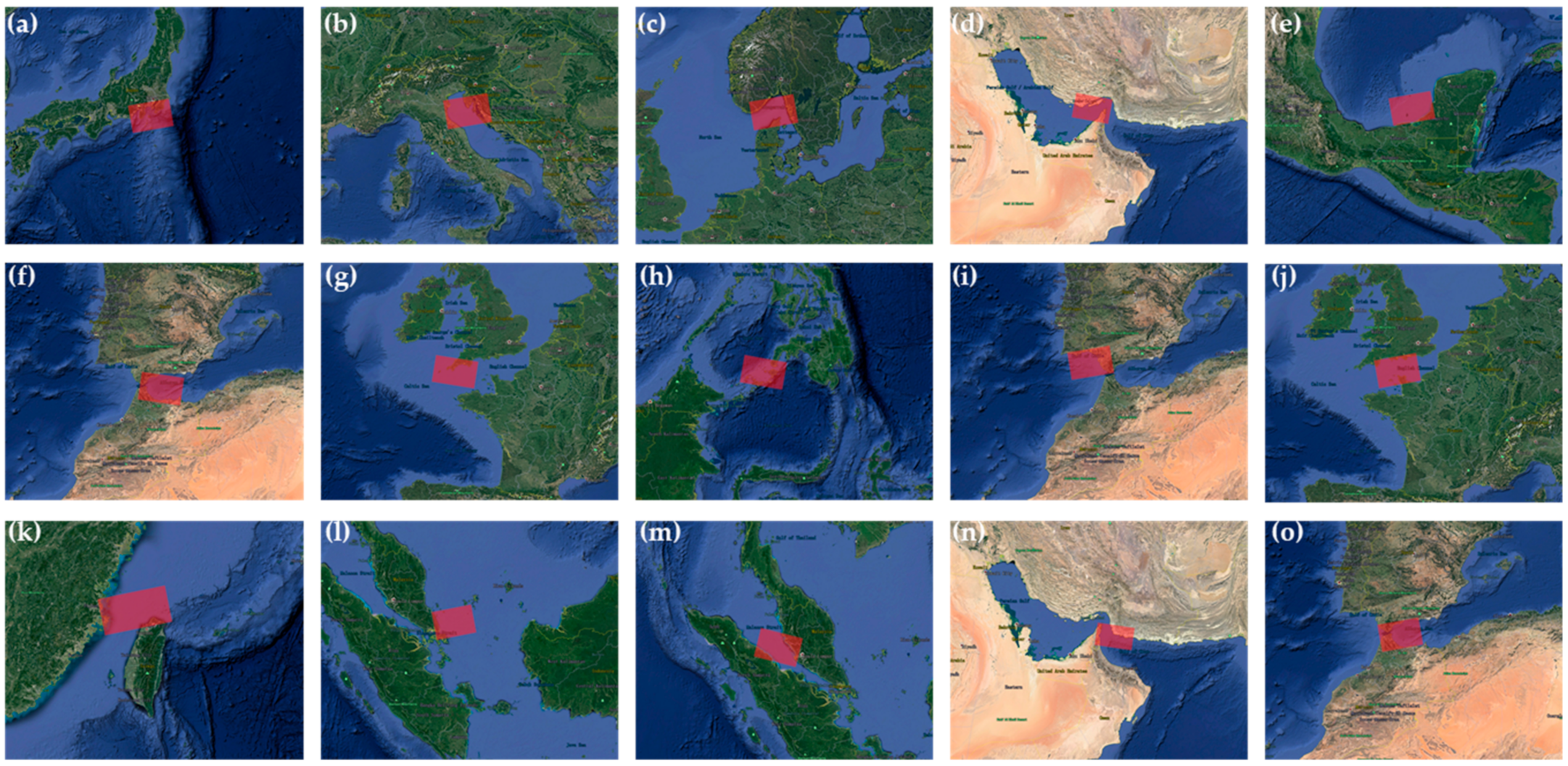
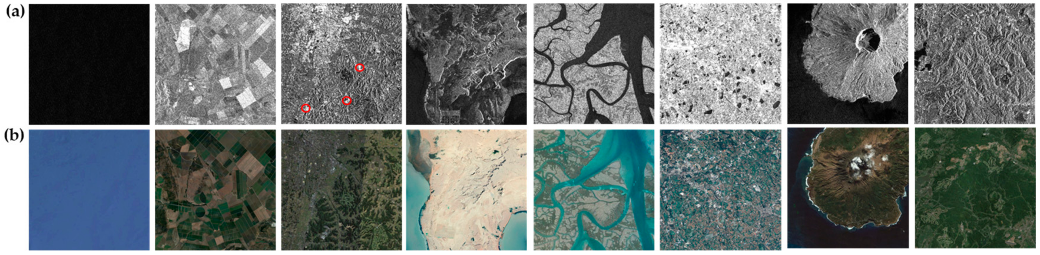
Large-scale background: Except AIR-SARShip-1.0, the other datasets did not consider large-scale practical engineering application of space-borne SAR. One possible reason is that small-size ship chips are beneficial to ship classification [7], but they contain fewer scattering information from land. Thus, models trained by ship chips will have trouble locating ships near highly-reflective objects in large-scale backgrounds [7]. Although images in AIR-SARShip-1.0 have a relatively large size (3000 × 3000 pixels), their coverage area is only about 9 km wide, which is still not consistent with the large-scale and wide-swath characteristics of space-borne SAR that often cover hundreds of kilometers, e.g., 240–400 km of Sentinel-1. In fact, ship detection in large-scale SAR images is closer to practical application in terms of global ship surveillance. Thus, we collect 15 large-scale SAR images with 250 km swath width to construct LS-SSDD-v1.0. See Section 4.1 for more details.
(ii)
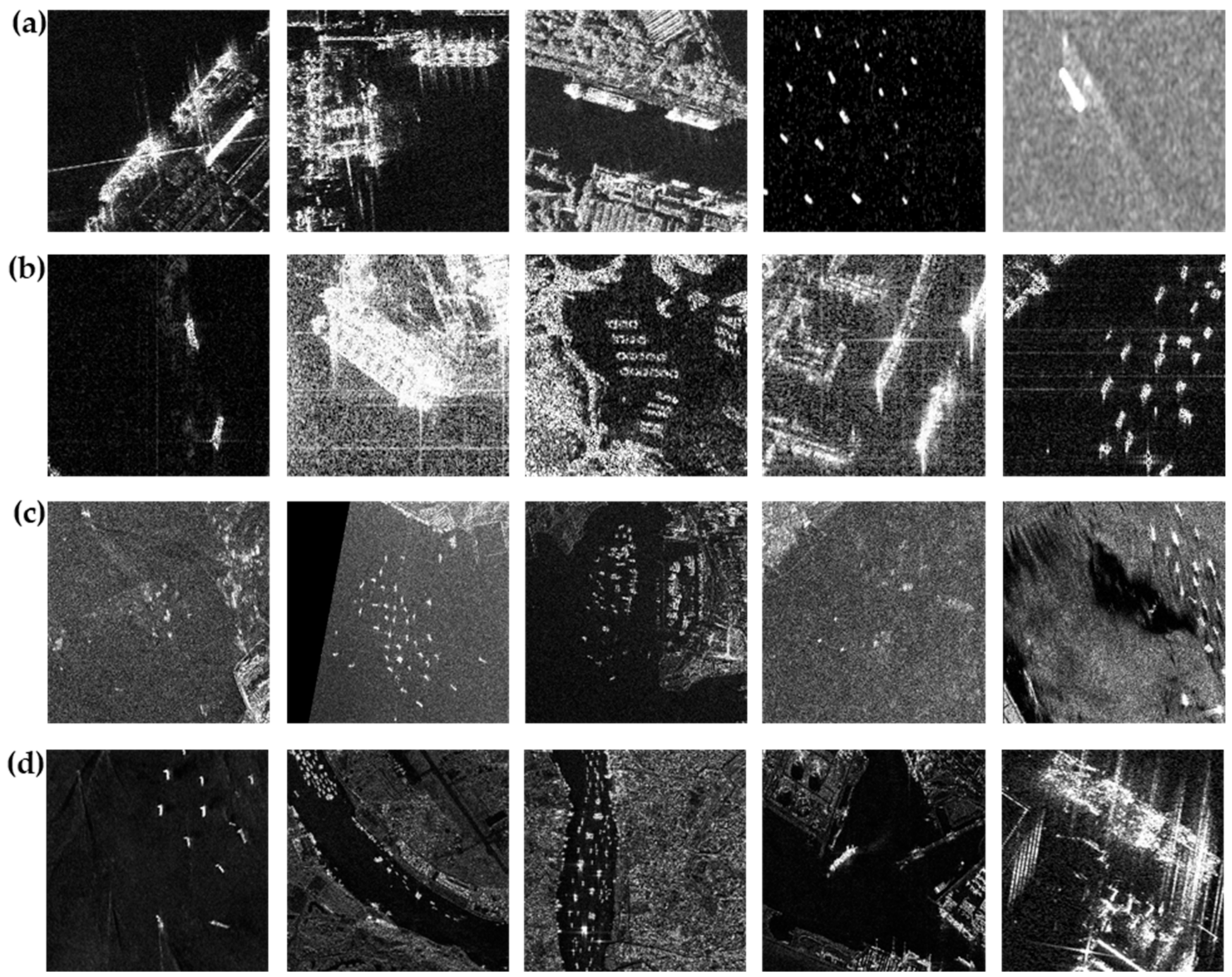
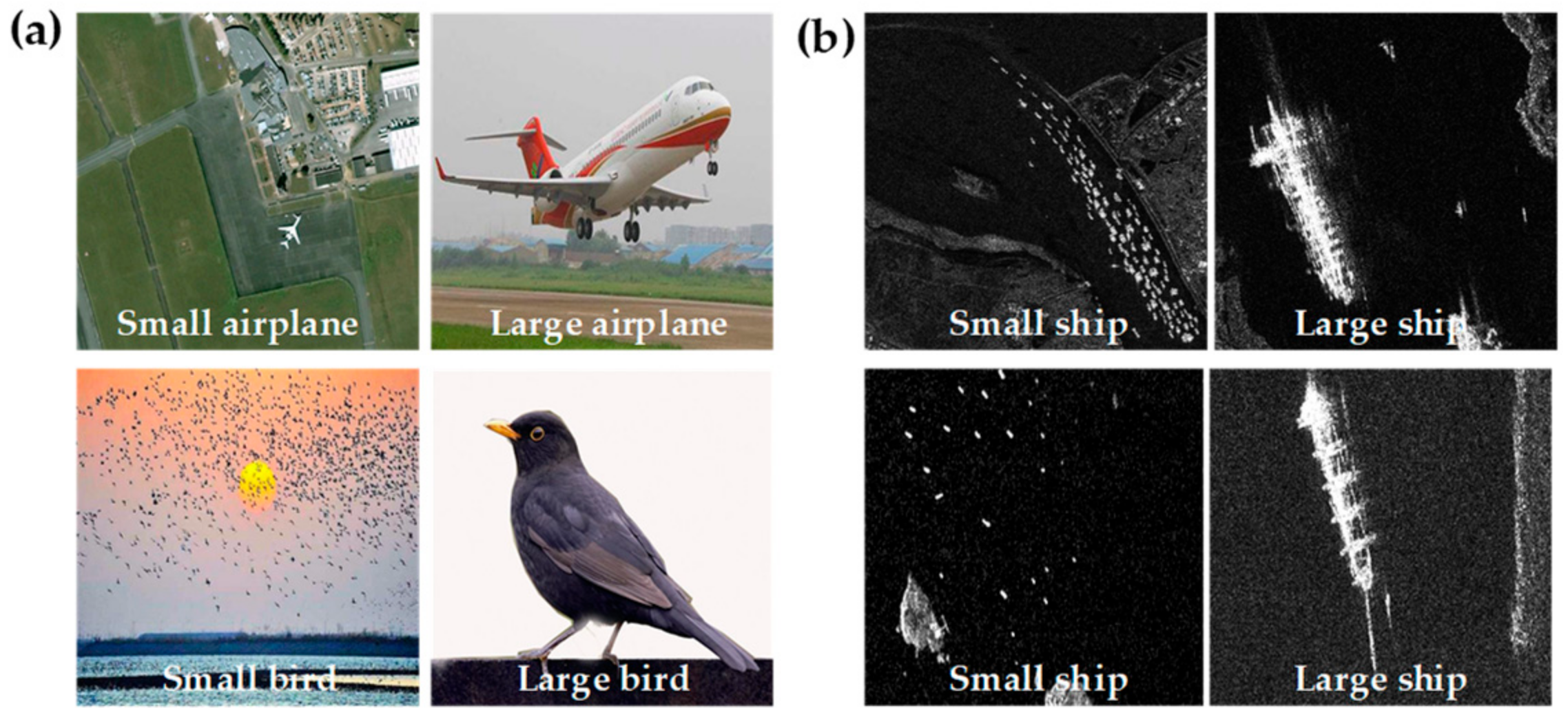
Small ship detection: The existing datasets all consider multi-scale ship detection [13,17], so there are many ships with different sizes in their datasets. One possible reason is that multi-scale ship detection is an important research topic that is one of the important factors to evaluate detectors’ performance. Today, using these datasets, there have been many scholars who have achieved great success in multi-scale SAR ship detection [13,17]. However, small ship detection is an another important research topic that has received much attention by other scholars [19,24,66] because small target detection is still a challenging issue in the deep learning community (it should be noted that “small ship” in the deep learning community refers to occupying minor pixels in the whole image according to the definition of the Common Objects in COntext (COCO) dataset [74] instead of the actual physical size of the ship, which is also recognized by other scholars [19,24,66].). However, at present, there is still lack of deep learning datasets for SAR small ship detection, so to make up for such a vacancy, we collect large-scene SAR images with small ships to construct LS-SSDD-v1.0. Most importantly, ships in large-scene SAR images are always small, from the perspective of pixel proportion, so the small ship detection task is more in line with the practical engineering application of space-borne SAR. See Section 4.2 for more details.
(iii)
Abundant pure backgrounds: In the existing datasets, all image samples contain at least one ship, meaning that pure background image samples (i.e., no ships in images) are abandoned artificially. In fact, such practice is controversial in application, because (1) for one thing, human intervention practically destroyed the raw SAR image real property (i.e., there are indeed many sub-samples not containing ships in large-scale space-borne SAR images); and (2) for another thing, detection models may not be able to effectively learn features of pure backgrounds, causing more false alarms. Although models may learn partial backgrounds’ features from the difference between ship ground truths and ship backgrounds in the same SAR image, false alarms of brightened dots will still emerge in pure backgrounds, e.g., urban areas, agricultural regions, etc. Thus, we include all sub-images into LS-SSDD-v1.0, regardless of sub-images contain ships or not. See Section 4.3 for more details.
(iv)
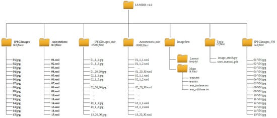
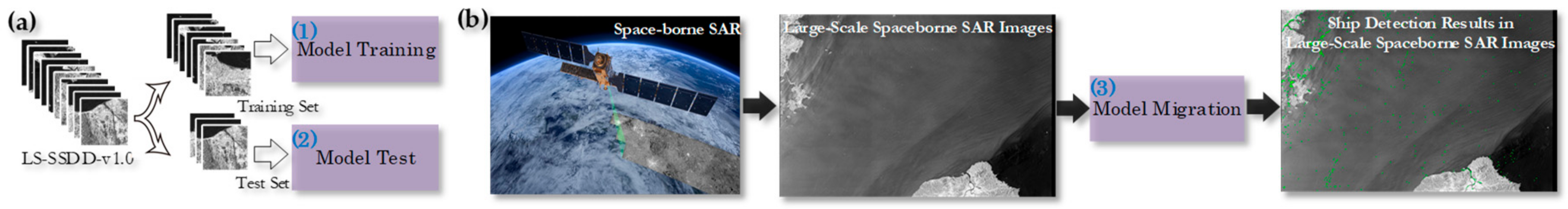
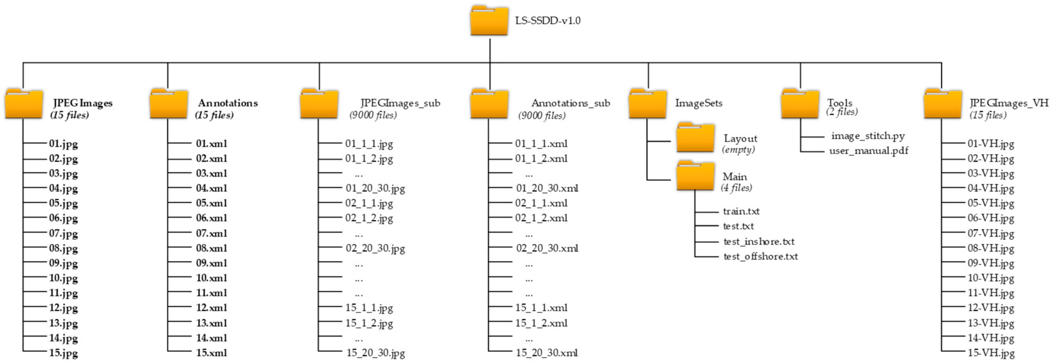
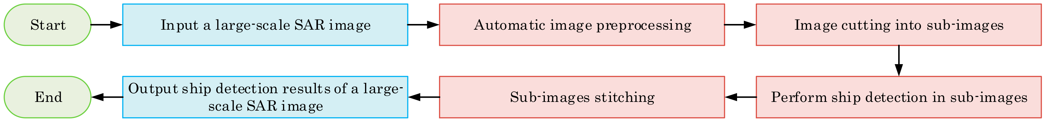
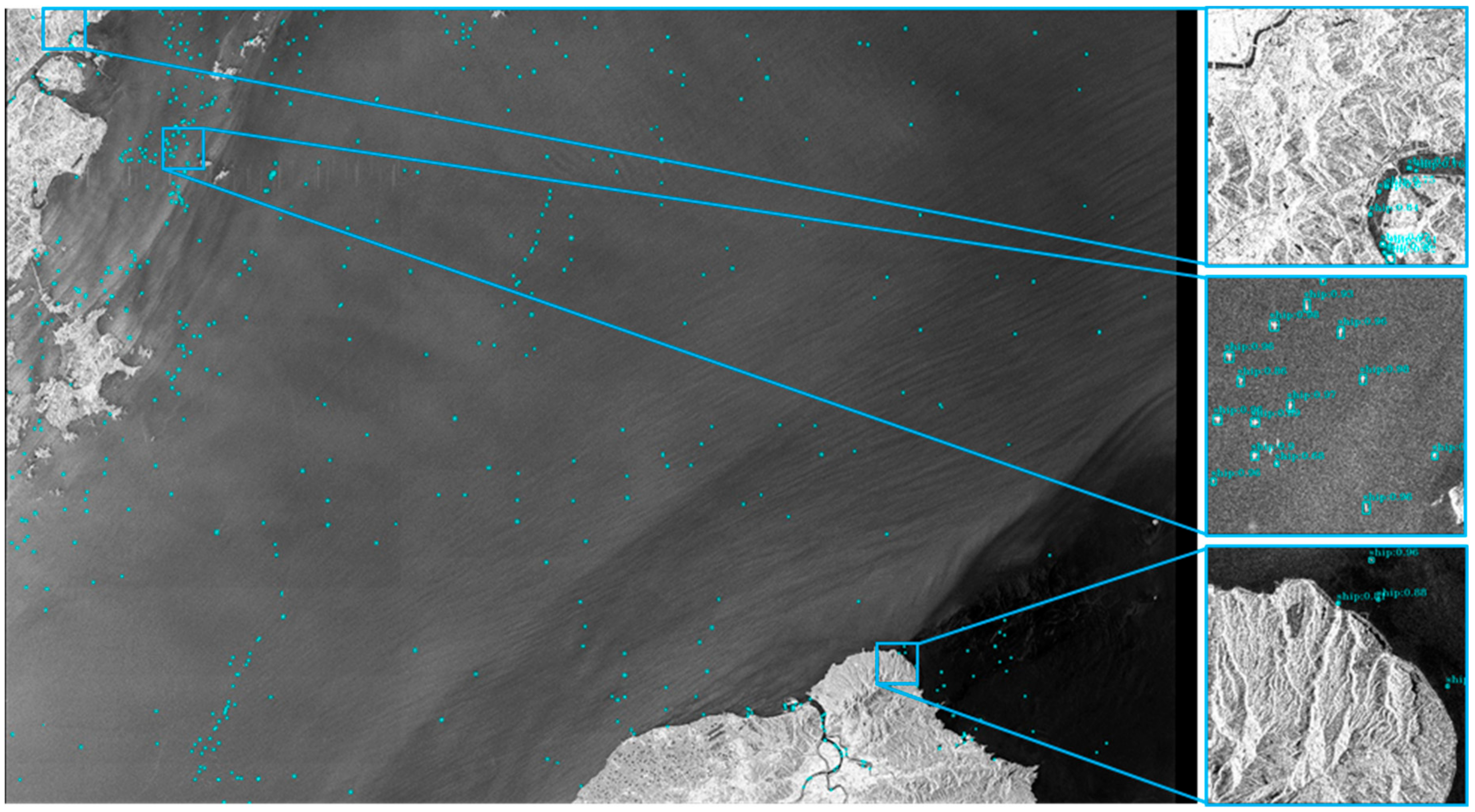
Fully automatic detection flow: In previous studies [1,2,3,4,6,10,34], many scholars have trained detection models on the training set of open datasets and then tested models on the test set. Finally, they always verified the migration capability of models on other wide-region SAR images. However, their process of authenticating model migration capability is a lack of sufficient automation for the domain mismatch between datasets and practical wide-region images. Thus, artificial interference is incorporated to select ship candidate regions from the raw large-scale images, which is troublesome and insufficiently intelligent, but if using LS-SSDD-v1.0, one can directly evaluate models’ migration capability because we keep the original status of large-scale space-borne SAR images (i.e., the pure background samples without ships are not discarded manually and the ship candidate regions are not selected by human involvement.), and the final detection results can also be better presented by simple sub-image stitching without complex coordinate transformation or other post-processing means, so LS-SSDD-v1.0 can enable a fully automatic detection flow without any human involvement that is closer to the engineering applications of deep learning. See Section 4.4 for more details.
(v)
Numerous and standardized research baselines: The existing datasets all provides research baselines (e.g., Faster R-CNN [75], SSD [76], RetinaNet [77], Cascade R-CNN [78], etc.), but (1) for one thing, the numbers of their provided baselines are all relatively a few that cannot facilitate adequate comparison for other scholars, i.e., two baselines for SSDD, six for SAR-Ship-Dataset, nine for AIR-SAR-Ship-1.0, and eight for HRSID; and (2) for another thing, they provided non-standardized baselines because these baselines are run under different deep learning frameworks, different training strategies, different image preprocessing means, different hyper-parameter configurations, different hardware environments, different programing languages, etc., bringing possible uncertainties in accuracy and speed. Although the research baselines of HRSID is standardized, they followed the COCO evaluation criteria [74], which is rarely used in the SAR ship detection community. Thus, we provide numerous and standardized research baselines with the PASCAL VOC evaluation criteria [79]: (1) 30 research baselines and (2) under the same detection framework, the same training strategies, the same image preprocessing means, almost the same hyper-parameter configuration, the same development environment, the same programing language, etc. See Section 4.5 for more details.
Moreover, based on abundant pure backgrounds, we also propose a PBHT-mechanism to suppress false alarms of land, and the experimental results can verify its effectiveness. LS-SSDD-v1.0 is a dataset according with practical engineering application of space-borne SAR, helpful for the progress of SAR intelligent interpretation technology. LS-SSDD-v1.0 is also a challenging dataset because small ship detection in the practical large-scale space-borne SAR images is a difficult task. It seems that the number of LS-SSDD-v1.0 is small because its image number is only 15. However, in fact, LS-SSDD-v1.0 is still a relatively big dataset because it contains 9000 sub-images. Although the image number in the SAR-Ship-Dataset seems to be bigger than ours (43,819 >> 9000), its image size is far small than ours (256 << 800 pixels) and their image samples also have a 50% overlap, causing (1) the detection speed decline for the duplicate detection in overlapping regions and (2) an inconvenience of subsequent results presentation in large-scale images. To be clear, some datasets, e.g., OpenSARShip [80], FUSAR [81], etc., were released for ship classification, e.g., cargo, tanker, etc., but this is not our focus, because this paper only focuses on ship location without the follow-up classification.
Especially, LS-SSDD-v1.0 is of significance, because (1) it can promote scholars to make extensive research into large-scale SAR ship detection methods with more engineering application value, (2) it can provide a data source for scholars who are focusing on the detection of small ships or densely clustered ships [19], and (3) it can motivate the emergence of higher-quality SAR ship datasets closer to engineering application and more in line with space-borne SAR characteristics in the future. LS-SSDD-v1.0 is available at https://github.com/TianwenZhang0825/LS-SSDD-v1.0-OPEN.
The main contributions of our work are as follows:
  • LS-SSDD-v1.0 is the first open large-scale ship detection dataset, considering migration applications of space-borne SAR and also the first one for small ship detection, to our knowledge;
  • LS-SSDD-v1.0 is provided with five advantages that can solve five defects of existing datasets.
The rest of this paper is as follows. Section 2 reviews related work. Section 3 introduces establishment process. Section 4 introduces five advantages. Experiments are described in Section 5. Results are shown in Section 6. Discussion is introduced in Section 7. A summary is made in Section 8.

2. Related Work

Table 1 shows the descriptions of the existing four datasets and our LS-SSDD-v1.0, as provided in their original papers [7,10,12,22]. Figure 2 shows some SAR image samples in them.

2.1. SSDD

In 2017, Li et al. [12] released SSDD from RadarSat-2, TerraSAR-X and Sentinel-1 with mixed HH, HV, VV, and VH polarizations, consisting of 1160 SAR images with 500 × 500 pixels containing 2358 ships, with various resolutions from 1 m to 15 m. Similar to PASCAL VOC [79], SSDD was established whose ground truths are labeled by LabelImg [3]. One image corresponds to an extensible markup language (XML) label. Regions with > 3 pixels are seen as ships, instead of AIS and Google Earth, so label errors may occur declining dataset authenticity. So far, scholars have proposed many SAR ship detection methods [1,2,3,4,5,6,8,13,14,15,16,17,18,19,20,21,29,32] on SSDD, but SSDD has careless annotation, repeated scenes, deficiency of sample number, etc., which hinders the further progress of research.
SSDD prophesied that deep learning would prevail, whose initial work has laid an important foundation. Later, as the update of deep learning object detectors, scholars realized that one must obtain more training data to enhance learning representation capability to further improve accuracy. As a result, the SAR-Ship-Dataset emerged.

2.2. SAR-Ship-Dataset

In March 2019, Wang et al. [30] released the SAR-Ship-Dataset from Gaofen-3, Sentinel-1, consisting of 43,819 small ship chips of 256 × 256 pixels, containing 59,535 ships, with various resolutions (3 m, 5 m, 8 m, 10 m, 25 m, etc.) and with single, dual and full polarizations. The ground truths are labeled by SAR experts. They did not draw support from AIS nor Google Earth, so the annotation process of their dataset relies heavily on expert experience, probably declining dataset authenticity. Moreover, the SAR-Ship-Dataset abandoned the samples without ships, but such practice (1) destroyed the large-scale space-borne SAR image property, i.e., there are indeed many samples not containing ships, and (2) may not effectively learn features of pure backgrounds. Although detectors can learn background features from the difference between ground truths and backgrounds in the same image, false alarms of brightened dots will still emerge in pure backgrounds.
The SAR-Ship-Dataset’s large number of images number can make models learn rich ship features. So far, scholars have reported research results on it, e.g., Cui et al. [14], Gao et al. [26], etc., but its image size is too small to satisfy the practical migration requirements, so AIR-SARShip-1.0 emerged.

2.3. AIR-SARShip-1.0

In December 2019, Sun et al. [22] released AIR-SARShip-1.0 from Gaofen-3 with 1-m and 3-m resolution and single polarization consisting of 31 images with 3000 × 3000 pixels in harbors, islands, reefs, and the sea surface under different conditions. They also labeled the ship ground truths based on expert experience, not drawing support from AIS or Google Earth. AIR-SARShip-1.0 provides the labels of the raw SAR images with 3000 × 3000 pixels, instead of those of their training sub-images. Although they have cut the raw SAR images into 500 × 500 pixel sub-images for network training, the final detection results are shown in the raw 3000 × 3000 pixel images, reflecting an end-to-end mode of the practical migration applications. That is, no matter what kind of image division mechanism (e.g., direct cutting, sliding window, visual saliency, etc.), they should provide the final ship detection results on the raw images, instead of small sub-images. However, their 3000 × 3000 pixel image size (only 9 km of swath width) still does not fully reflect SAR images’ wide-swath characteristic. Moreover, its total quantity of images for network training is relatively small (1116 sub-images), inevitably bringing about inadequate learning, and even leading to training over-fitting, which reduces the models’ generalization capability. Although they used data augmentation, e.g., dense rotation, image flipping, contrast enhancement, random scaling, etc., to alleviate this problem, data augmentation can only learn limited ship features based on limited data, and it is obvious that it is not definitely a better choice if they do not expand the number of datasets. In addition, according to our observation, SAR images in AIR-SARShip-1.0 seem to be of relatively low-quality compared with SSDD and SAR-Ship-Dataset, e.g., severe speckle noise, intense image defocus, etc., possibly coming from the modest imaging algorithms for the raw SAR data, which probably declines the feature extraction of real ships.
AIR-SARShip-1.0 inspired our work (i.e., design a dataset in line with the actual migration application.). So far, Fu et al. [35] and Gao et al. [27] have reported their research results based on AIR-SARShip-1.0. However, the SAR image quality of AIR-SARShip-1.0 is modest, possibly bringing about certain resistance for other scholars’ further studies. As a result, HRSID emerged.

2.4. HRSID

In July 2020, Wei et al. [7] released HRSID from Sentinel-1 and TerraSAR-X, for ship instance segmentation including ship detection. There are 5604 SAR images with 0.5 m, 1 m, and 3 m resolutions; 800 × 800 pixels; and HH, HV, and VV polarization in HRSID, containing 16,951 ships. It is worth noting that they labeled the ship ground truths in SAR images, with the help of Google Earth, which is a progress compared to SSDD, SAR-Ship-Dataset, and AIR-SARShip-1.0, but AIS is still not considered in their work. Moreover, HRSID also abandoned the pure background samples by manual intervention, which leads to the emergence of many false alarm cases of brightened dots in some pure background SAR images, e.g., urban areas, agricultural regions, etc.
HRSID reminds us that small ship chips are beneficial to ship classification [7] because these ship chips contain fewer scatterings from land, so models trained by ship chips may have trouble locating ships near highly reflective objects, which inspired us to consider large-scale SAR ship detection.

3. Establishment Process

3.1. Step 1: Raw Data Acquisition

We download the 15 raw Sentinel SAR data from the Copernicus Open Access Hub [82] in busy ports, straits, river areas, etc. Table 2 shows the detailed information of the 15 raw Sentinel-1 SAR data. From Table 2, LS-SSDD-v1.0 is composed of Sentinel-1 images in the interferometric wide swath (IW) mode, which is the main Sentinel-1 mode to acquire data in areas of maritime surveillance (MS) interest [9]. We choose ground range multi-look detected (GRD) data for most intensity-based applications, instead of single-look complex (SLC) data for interferometric applications [83]. The default polarimetric combination for Sentinel-1 images acquired over areas of maritime interest is (VV-VH) [83]. For incidence angles in the range of 30° to 45°, which are characteristic for Sentinel-1 IW, vessels generally exhibited higher backscattering values in the co-polarization channel (VV), while in the cross-polarization channel (VH), the backscattering values were lower [9,83]. In addition, we also note that there is a special type of instrumental artifact in Sentinel-1 VH polarization images [84], probably coming from the radio frequency interference (RFI) of instrumental artifacts [84]. The intensity of RFIs could be as strong as ships, making it difficult to distinguish them using methods based on intensity information. Given the above, we choose VV co-polarization to perform actual ship annotation. In particular, for cross-polarization, the ship RCS is smaller, but the clutter is below the noise floor; the cross-polarization case is noise limited [83]. There are significant benefits to using cross-polarization, especially for acquisitions at smaller incidence angles [83]. Furthermore, cross-polarization provides more uniform ship detection performance across the image swath since the noise floor is somewhat independent of incidence angle [83]. Therefore, we also provide the 15 raw large-scale SAR images with VH polarization in the LS-SSDD-v1.0 source documents for possible further research in the future, which possess the same ship label ground truths as VV polarization.
Figure 3 shows their coverage areas. In Figure 3, the 15 raw Sentinel SAR data has large-scale and width swath characteristics (250 km > 9 km of AIR-SAR-Ship-1.0 > 4 km of HRSID > 0.4 km of SAR-Ship-Dataset), covering a large area of sea, straits, ports, shipping channels, etc. Moreover, their image sizes are all relatively large, about 26,000 × 16,000 pixels on average, compared to other datasets.
We used the Sentinel-1 toolbox [85] to help imaging to obtain 15 tag image file format (TIFF) files with 16-bit physical brightness or grey levels, where all images are processed by geometrical rectification, radiometric calibration and de-speckling. Moreover, as demonstrated in the scientific literature [83], the minimum detectable ship length for the groups of single beam modes is about 25–34 m for 30° to 45° incidence angle [80,83] (~1.46 dB intensity contrast [83] similar to ice), and it also decreases with increasing incidence angle, which illustrates the importance of incidence angle in reducing the background ocean clutter level. More details of Sentinel-1 can be found in Torres et al. [83].
Finally, the European Space Agency (ESA) provided the specific shooting time of Sentinel-1 satellite in their annotation files, and moreover, with the help of the Sentinel-1 toolbox, we can also obtain the latitude and longitude information of the surveyed areas. Thus, the above exact time and accurate geographical location will be convenient for the follow-up AIS consultation and Google Earth correction. Thus far, the raw 15 large-scale SAR images with the TIFF file format have been obtained.

3.2. Step 2: Image Format Conversion

To keep a same image format as PASCAL VOC [79], we convert the 15 raw tiff files into the Joint Photographic Experts Group (JPG) files, and we use the Geospatial Data Abstraction Library (GDAL) [86], a translator library for raster and vector geospatial data formats, to accomplish such format conversion. Thus far, the raw 15 large-scale SAR images with the .jpg file format were obtained.

3.3. Step 3: Image Resizing

From Table 2 in Section 3.1, the raw 15 large-scale SAR images are provided with different sizes, but they are all about 26,000 × 16,000 pixels on average. To generate more uniform training samples so as to facilitate the image cutting in Section 3.4, we resize these images with uniform sizes into 24,000 × 16,000 pixels by resampling, where 24,000 and 16,000 can be divisible by 800 which is a moderate size for most deep learning detection models. Our such practice is also the similar as HRSID [7]. Thus far, the raw 15 large-scale SAR images with 24,000× 16,000 pixels have been obtained.

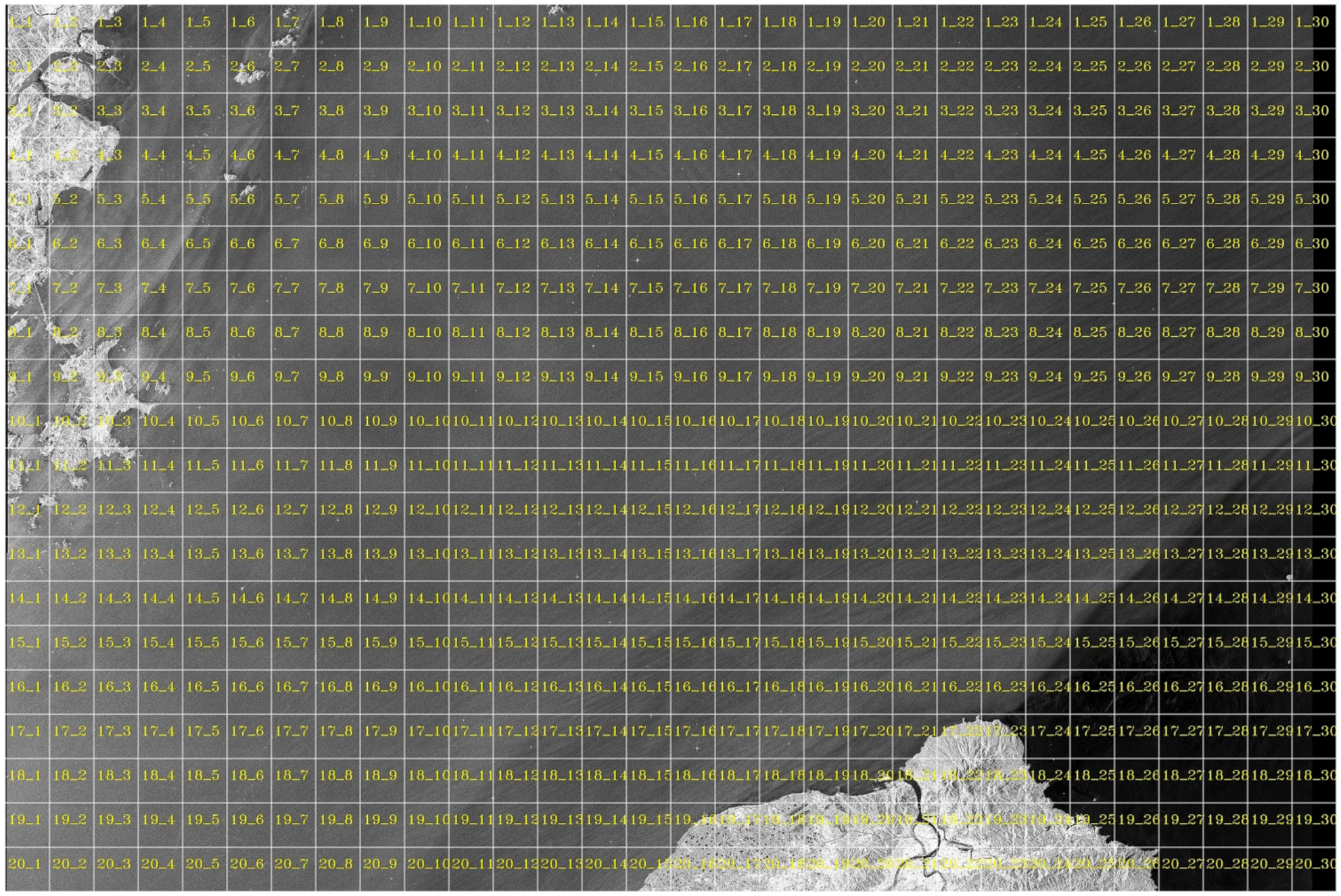
3.4. Step 4: Image Cutting

Figure 4 shows the process of image cutting. In order to facilitate network training, these 15 large-scale SAR images with 24,000 × 16,000 pixels are directly cut into 9000 sub-images with 800 × 800 pixels without bells and whistles (marked in white lines). As a result, 600 sub-images for each large-scale image are obtained. In Figure 4, the small 600 sub-images from each large-scale image are, respectively, numbered as N_R_C.jpg (marked in yellow numbers), where N denotes the serial number of the large-scale image, R denotes the row of sub-images, and C denotes the column. For instance, as is shown in Figure 4 and taking the 11.jpg as an example, the size of the original large-scale SAR images is 24,000 × 16,000 pixels, and after cutting, 600 sub-images with 800 × 800 pixels are generated that are numbered as from 1_1.jpg to 1_30.jpg, from 2_1.jpg to 2_30.jpg, …, and from 20_1.jpg to 20_30.jpg, which means the division of 20 rows and 30 columns.
Finally, the total 9000 sub-images are generated for network training and test in the LS-SSDD-v1.0 dataset. In LS-SSDD-v1.0, we select the first 10 large-scale images as a training set and the remaining five images as a test set. In other words, the first 6000 small sub-images coming from 01.jpg to 10.jpg are selected as a training set, and the remaining 3000 sub-images coming from 11.jpg to 15.jpg as a test set. Different from the sliding window mechanism used in SAR-Ship-Dataset, we adopt the direct and simple cutting mechanism that is the similar as AIR-SARShip-1.0 to produce sub-images, because (1) for one thing, such direct cutting mechanism is more efficient and concise, and also can avoid repeated detection of the same ship in multiple sub-images (e.g., 128 pixels are shifted over both columns and lines during the sliding window, leading to a 50% overlap of adjacent ship chips in the work of Wang et al. [30]). As a result, the total detection speed can be improved. (2) For another thing, our practice is also convenient for the subsequent presentation of large-scene SAR ship detection results, i.e., only the simple image stitching operation is needed, without more complicated post-processing of ship coordinate transformation, from small sub-images to large-scale images.
Regardless of whether the sub-images contain ships or not, we all add them to our LS-SSDD-v1.0 dataset for network training and test, because (1) for one thing, our such practice complies with the raw SAR image property because there are indeed many samples not containing ships in the practical migrating applications of large-scale space-borne SAR images, and (2) for another thing, detection models can effectively learn features of many pure backgrounds to suppress some false alarms, e.g., some brightened dots in urban areas, agricultural regions, mountain areas, etc., according to our findings in Section 7. Thus far, these 9000 sub-images have been obtained.

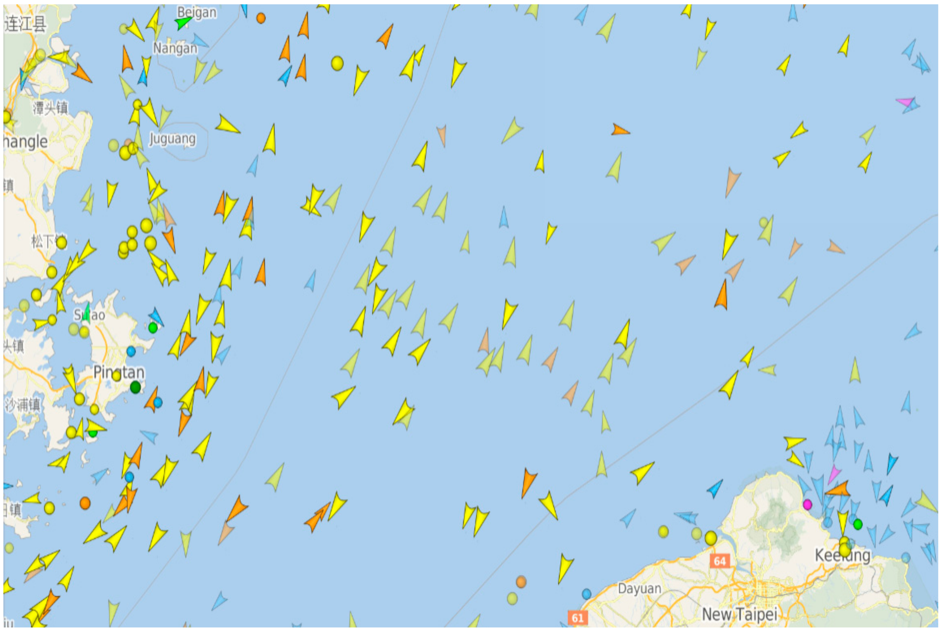
3.5. Step 5: AIS Support

Before labeling the ship ground truths, SAR experts firstly draw support from AIS to roughly determine the possible positions of ships in the large-scale SAR images, according to the exact time and the accurate geographical location of the raw SAR data, introduced in Section 3.1. Figure 5 shows the AIS messages. In Figure 5, the inshore AIS systems and satellite AIS systems are both employed to get more comprehensive ship information.
In addition, it should be noted that AIS can automatically broadcasts information from the vessel to an AIS ship receiver or an inshore receiver by very high frequency (VHF), but they can only work in a limited geographical space [87] (about 200 nautical miles) coming from their limited base station (BS) operating distance. In other words, in fact, some ships far away from land cannot be searched by inshore VHF receivers, and moreover, although the satellite AIS systems can find these ships, there is still a long time delay due to the periodic motion of the satellite around the Earth. Therefore, it is difficult to fully match the SAR images with a very accurate AIS information at the corresponding time and corresponding locations, but we have tried our best to narrow such gap. Moreover, in fact, it is not fully feasible to mark ships if merely using AIS information because many small ships with <300 tons mass are rarely installed AIS, according to our investigation [88]. Therefore, we also draw support from the Google Earth for our annotation correction, which will be introduced in Section 3.7. Thus far, SAR experts have obtained some prior information from AIS.

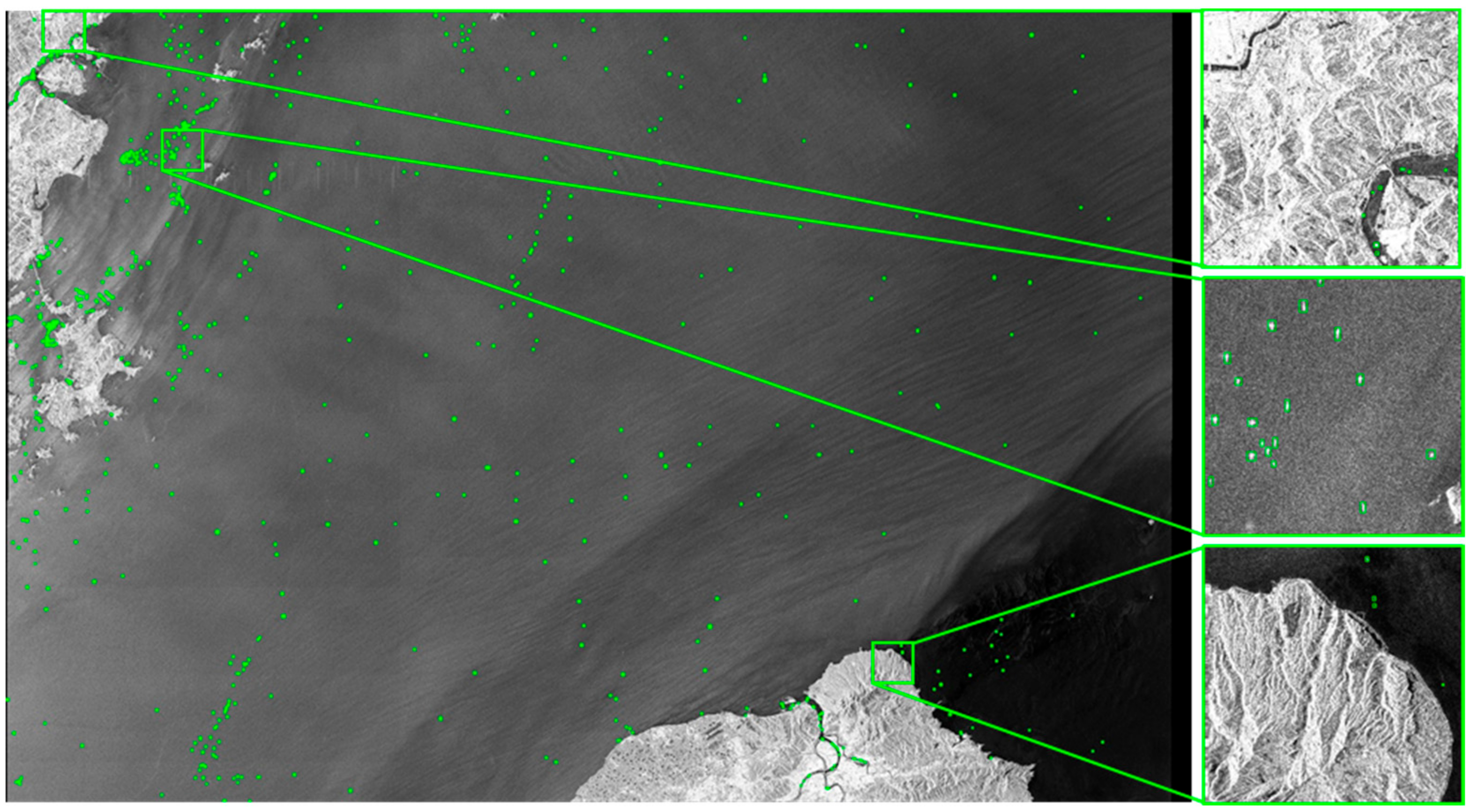
3.6. Step 6: Expert Annotation

The ship ground truths of the 9000 sub-images are annotated by SAR experts, using LabelImg. In the expert annotation process, AIS and Google Earth both provide some suggestions for some controversial areas, e.g., some islands, ports facilities similar to ships, etc. For prominent marine SAR reflectors, in most cases, we can distinguish them easily according to their shape feature difference with real ships. If some prominent marine SAR reflectors are so similar to ships that we cannot discriminate them based on significant geometric features, we draw support from Google Earth to determine their real conditions. For example, there is a prominent marine SAR reflector in the Google Earth optical images through visual observation, so we remove it in the SAR images.
During the annotation process, if there are obvious V-shape wake and scattering point defocusing phenomenon, we regard these strong scattering points as moving ships, and the others are regarded as stationary/moored ships. In other words, as long as the speed of the ship is not large enough to appear in the above two situations, we think that they are stationary. Although our practice is rough, it is in line with the actual situation to a certain extent, because in such wide-region space-borne Sentinel-1 SAR images, compared to the satellite with a high-speed operation, the speed/velocity of ships is far lower, so in most cases, they can be regarded as stationary targets, which is obviously different from air-borne SAR according to our experience. For ships with obvious wakes and ships with scattering point defocusing, we do not include their wake pixels and defocusing pixels into the ship ground truth rectangular box. In other words, similar to the other existing datasets, we only use the geometrical properties of ships or the areas around them to act as the salient features of ships based on visual enhanced mechanism. Moreover, for ships with different headings or courses, we use the maximum and minimum pixel coordinates from pixels of ship hulls to draw the ship ground truth rectangular box. In other words, similar to the other datasets, we only use rectangular box to locate the center point of the ship, not considering the direction estimation of rotatable boxes. Therefore, a ship ground truth box may have ships in different headings or courses, which means that as long as these ships with different courses have similar center coordinates, they are measured by a same rectangular box.
Moreover, in SAR images, ships and icebergs typically have a stronger backscatter response than the surrounding open water, so icebergs that occur in a large variety of sizes and shapes impose additional challenge to our ship annotation process. First, according to the geographical locations and shooting time (the determination of the area season) of the original SAR images, drawing support from the World Glacier Inventory (WGI) [89], we determined that the covered area belongs to an open sea area where icebergs rarely exist or a complex sea-ice area where icebergs often exist. For the former, we do not consider icebergs effects that hardly exist. For the latter, we use intensity and shape features to discriminate ships and icebergs or ice floes, inspired from Bentes et al. [90], because they generally have the obvious differences in the dominant scattering mechanism [90].
According to the shooting time and geographical positions of SAR images, one can also consult the satellite images of the corresponding weather conditions including precipitation in the website of the World Weather Information Service from the World Meteorological Organization (WMO) [91]. In addition, for different water surface phenomena that comes from different weather conditions, we do not pay too much attention to it because the gray level change of image backgrounds possibly from different sea clutter distribution is still not obvious in contrast to high-intensity ships. Certainly, if there is extreme weather in a sea area (e.g., typhoon), we will pay more attention to inshore ships that may be less likely to go to sea in extreme weather conditions, so they often park at ports side by side densely.
Figure 6 shows the expert annotation process. In Figure 6a, the image axis x and y are marked in orange. From Figure 6a, in LS-SSDD-v1.0, we employ a rectangular box to represent a ship (marked in green), where its top-left vertex A (xmin, ymin) (marked in black) and bottom-right vertex B (xmax, ymax) (marked in red) are used to locate the real ship. After the rectangle box has been drawn, the LabelImg annotation tool will pop up a dialog box to prompt for the category information (i.e., ship in LS-SSDD-v1.0). After the category information is input successfully, the xml label file, as is shown in Figure 6b, will be generated automatically. In Figure 6b, the blue rectangle mark refers to the image information including the width, height, and depth; the green rectangle mark refers to the category information (i.e., ship in LS-SSDD-v1.0); and the red rectangle mark refers to the ship ground truth box, which are denoted as xmin, ymin, xmax, and ymax.
Different from HRSID, which employs polygons to describe ships because they need to implement ship segmentation task and in the deep learning community, the ship detection task generally is always described by rectangular boxes. Finally, in order to ensure the correctness of ship labels as much as possible, we also invite more experts to provide technical guidance. Thus far, 9000 label files with the xml format have been obtained.

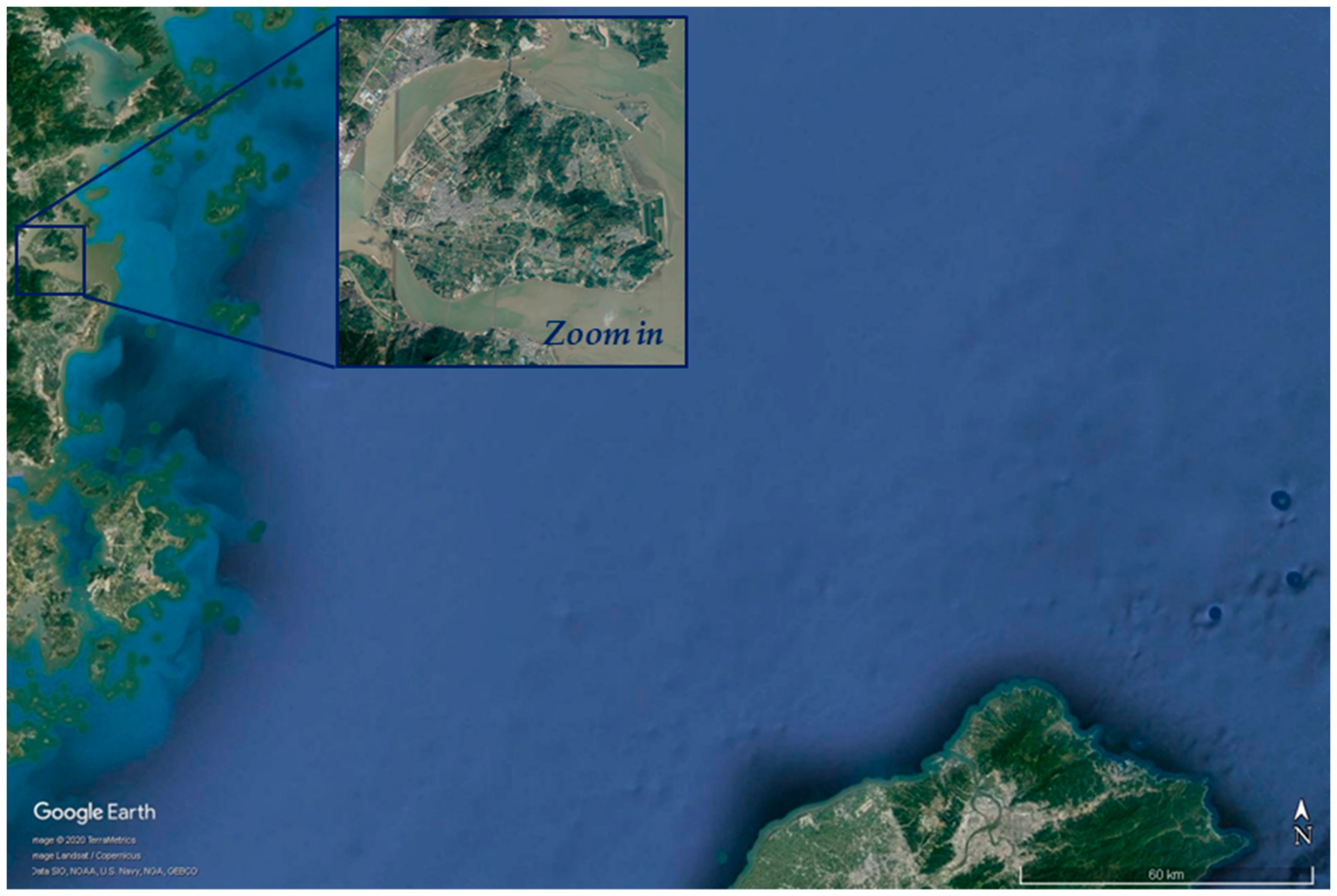
3.7. Step 7: Google Earth Correction

To ensure the authenticity of the dataset as much as possible, we also utilize Google Earth for more careful inspection. In Google Earth, we choose the closest time to approximately match the shooting time of SAR images. Figure 7 shows a Google Earth optical image of 11.jpg SAR image in the same coverage areas. In our correction process, appropriate enlargement of images, i.e., zoom in (marked in blue box in Figure 7) is needed to obtain more detailed geomorphological information and ocean conditions. Moreover, we find that some islands and reefs are labeled as ships by mistake, so we performed their correction, which shows Google Earth correction plays an important role.
It needs to be clarified that Google Earth is merely used for annotation correction, and in fact, it cannot provide fully accurate ship information because there is still a time gap between its optical images shooting time and SAR images. Moreover, such time gap is objective and cannot be overcome unless Google Corporation updates maps in time. Yet, LS-SSDD-v1.0 is still superior to other datasets because they rarely considered Google Earth correction. Thus, finally, we draw support from Google Earth to identify islands or docks whose locations may not change with time based on visual observation, so as to (1) check some areas that are easy to label incorrectly and (2) correct wrong labels.
To here, we complete the dataset establishment process. Figure 8 shows ground truths of 11.jpg (marked in green). Compared with other datasets, from Figure 8, it is obvious that LS-SSDD-v1.0 has the characteristics of large-scale background and small ship detection.
Finally, in order to facilitate scholars to use LS-SSDD-v1.0, we provide a file preview as is shown in Figure 9. In Figure 9, there are seven file folders in the root directory of LS-SSDD-v1.0 (a compressed package file with zip format): (1) JPEGImages, (2) Annotations, (3) JPEGImages_sub, (4) Annotations_sub, (5) ImageSets, (6) Tools, and (7) JPEGImages_VH.
(1) JPEGImages in Figure 9 has 15 files, which contain the 15 raw large-scale space-borne SAR images that are numbered as from 01.jpg to 15.jpg. The size of these SAR images is 24,000 × 16,000 pixels.
(2) Annotations in Figure 9 has 15 files, which contain the 15 ground truth label files of real ships that are numbered as from 01.xml to 15.xml. These labels files are in line with PASCAL VOC standard shown in Figure 6b.
(3) JPEGImages_sub in Figure 9 has 9000 files, which contain 9000 sub-images with 800 × 800 pixels that are obtained from the raw 15 large-scale SAR images based on image cutting numbered as from 1_1.jpg to 1_30.jpg, from 2_1.jpg to 2_30.jpg, …, and from 20_1.jpg to 20_30.jpg, as introduced in Section 3.4. In addition, these sub-images are numbered as N_R_C.jpg, where N denotes the serial number of the large-scale image, R denotes the row of sub-images, and C denotes the column. It should be noted that these sub-images are actually used in our network training and test in this paper, due to limitation of GPU memory. If there are some distributed high performance computing (HPC) [8] GPU servers, one can direct train the raw 24,000×16,000 pixels large-scale SAR images.
(4) Annotations_sub in Figure 9 contains 9000 label files of ship ground truths numbered as 1_1.xml to 1_30.xml, 2_1.xml to 2_30.xml, …, and 20_1.xml to 20_30.xml, respectively, corresponding to 9000 sub-images with the same file number.
(5) ImageSets in Figure 9 contains two file folders (Layout and Main). Layout is used to place ship segmentation labels for future version updates, and Main is used to place the training set and test set division files (train.txt and test.txt). Similar to HRSID [7], regarded images containing land as inshore samples, we follow this means to divide the test set into a test inshore set and a test offshore set (test_inshore.txt and test_offshore.txt) to facilitate future studies of other scholars [48,49] who focus on inshore ship detection, because it is more difficult to detect inshore ships than offshore ships.
(6) Tools in Figure 9 contains a Python tool file named as image_stitch.py to stitch sub-images’ detection results into the original large-scale SAR image. We also provide a user manual for other scholars’ easier use, named as user_manual.pdf. In addition, in the user_manual.pdf, one can also link to and obtain additional information about the images by searching the specific product IDs of these 15 raw SAR images in the Copernicus Open Access Hub website [82].
(7) JPEGImages_VH in Figure 9 has 15 files, which contain the 15 raw large-scale space-borne SAR images with VH cross-polarization numbered as from 01_VH.jpg to 15_VH.jpg that is used for future dual polarization research. In addition, these 15 VH cross-polarization SAR images possess the same label ground truths as VV co-polarization. In this paper, we only provide the research baselines of the VV co-polarization.

4. Advantages

4.1. Advantage 1: Large-Scale Backgrounds

The capability to cover a wide area is a significant advantage of space-borne SAR, but previous datasets were always provided with limited detection backgrounds that may be not a best choice for the practical migration application in engineering. In fact, in general, small ship slices are relatively appropriate for ship classification [7] due to their obvious shapes, outlines, sizes, textures, etc., but they contain fewer scattering information from land, islands, artificial facilities, etc., negatively affecting the practical detection [7]. For the practical space-borne SAR ship detection task, in most cases, one always needs to detect ships in the large-scene SAR images so as to provide wide-range and all-round ship monitoring in the Earth, which is also recognized by Cui et al. [14] and Hwang et al. [58], so we collect SAR images with large-scale backgrounds to establish LS-SSDD-v1.0.
Table 3 shows the background comparison with other existing datasets. From Table 3, LS-SSDD-v1.0′s image size is the largest. Moreover, from Figure 2 and Figure 8, LS-SSDD-v1.0′s coverage areas are also the largest. Thus, LS-SSDD-v1.0 is closer to the practical migration application of wide-region global ship detection in space-borne SAR images, compared to the other four existing datasets. Finally, in Table 3, it should be noted that “image size” refers to the size of image samples in the dataset files that are provided by their publishers.

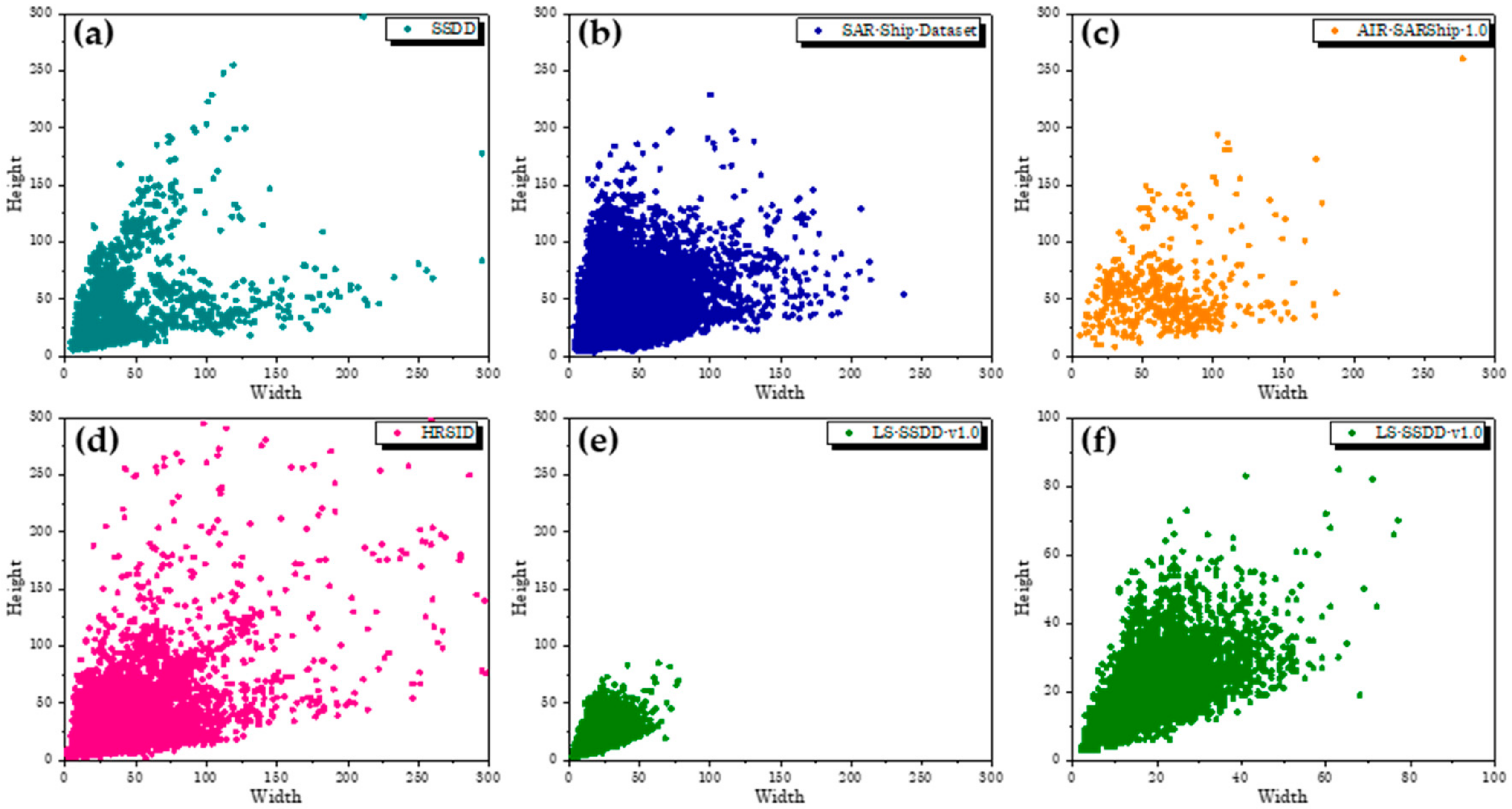
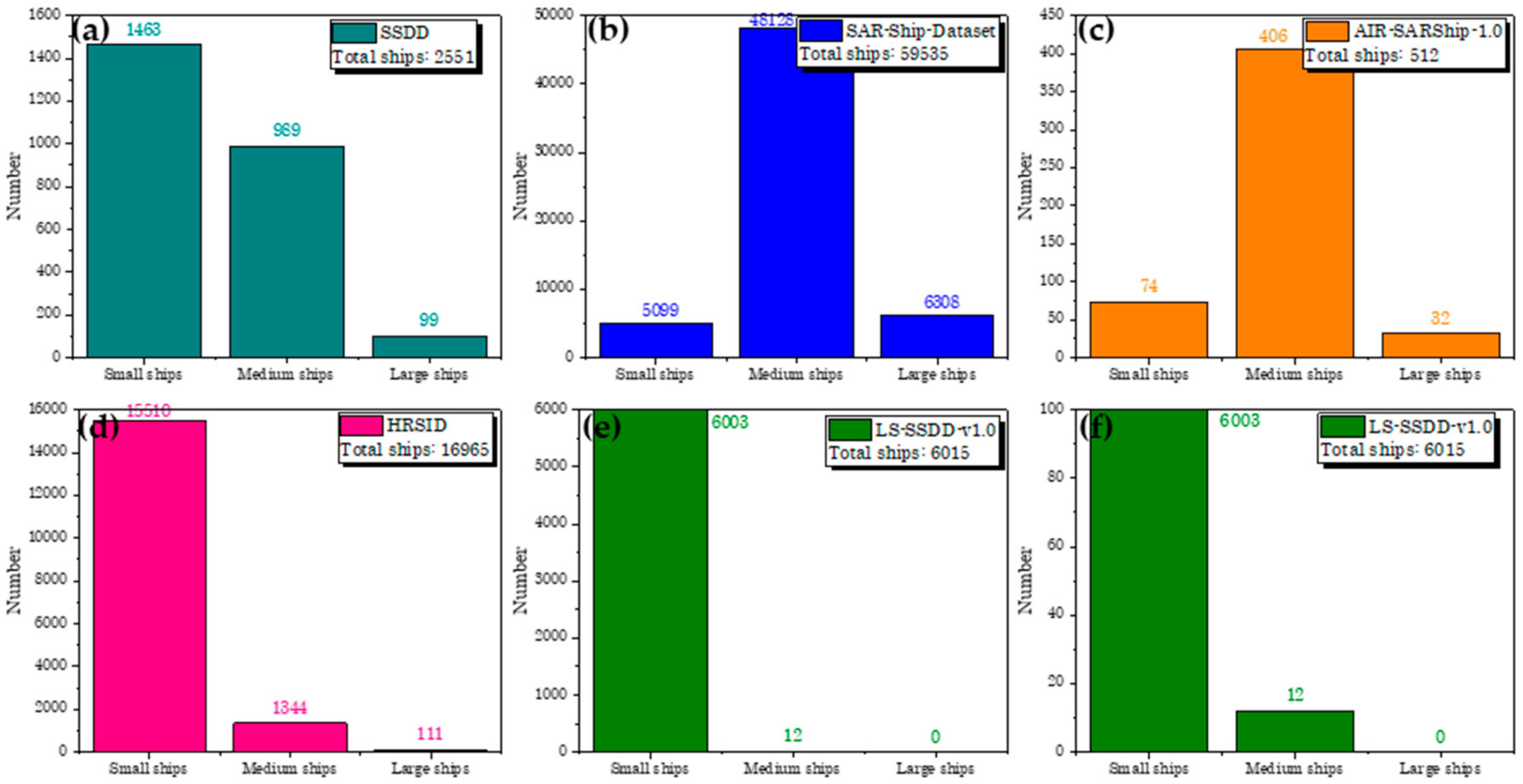
4.2. Advantage 2: Small Ship Detection

LS-SSDD-v1.0 can also be used for SAR small ship detection, and there are also two types of benefits: (1) in fact, ships in large-scale Sentinel-1 SAR images are always rather small from the perspective of occupied pixels (not real physical size), so LS-SSDD-v1.0 is closer to the practical engineering migration application; and (2) today, SAR small ship detection is also an important research topic that has received significant attention from many scholars [19,24,66], but there is still a lack of datasets that are used specifically to address this problem among open reports, so LS-SSDD-v1.0 can also compensate for such vacancy.
Special attention needs to be paid to is that in the deep learning community, “small ship” refers to occupying minor pixels in the whole image based on the definition of the COCO dataset [74], instead of real ship physical size (i.e., ship length and ship breadth). Figure 10 is the intuitive schematic diagram of small ship detection. For example, in nature, the airplane size is rather large, while in Figure 10a, the airplane in the first image is often regarded as a small one, but the airplane in the second image can also often regarded as a large one. In addition, in nature, bird size is often rather small, while in Figure 10a, the birds in the third image are often regarded as small ones, but the bird in the fourth image can also often be regarded as a large one. Therefore, for SAR ship detection, in Figure 10b, the ships in the first and the third images are regarded as small ships; meanwhile, the ships in the second and the fourth images can also often be regarded as large ships. To sum up, ship pixel ratio among the whole image is used to measure the ship size, instead of the physical sizes in meters. Up to now, many other scholars [19,24,66] have adopted this definition, and the existing other datasets are also based on this definition, so in this paper, we follow the usual practice. In other words, for deep learning object detection, we do not pay special attention to the specific resolution of images in meters or centimeters; on the contrary, we merely focus on the pixel proportion of the real object in the whole image, i.e., the relative pixel size, instead of the physical size.
Table 4 shows the ship pixel size comparison with the other existing datasets. From Table 4, the average ship area of LS-SSDD-v1.0 is only 381 pixels2, which is far smaller than others (i.e., 381 << 1134 < 1808 < 1882 < 4027), and the largest ship area is only 5822 pixels2, which is far smaller than others (i.e., 5822 << 26,703 < 62,878 < 72,297 < 522,400). Moreover, if we calculate the proportion of ship pixels among the whole image pixels based on average pixels2, ships in LS-SSDD-v1.0 will be greatly smaller than others. If we can take the average pixels2 as an example, then we can find that 381/(24,000 × 160,00) = 0.0001% of LS-SSDD-v1.0 << 4027/(3000×3000) = 0.0447% of AIR-SARShip-1.0 < 1808/(800 × 800) = 0.28% of HRSID < 1882/(500 × 500) = 0.75% of SSDD < 1134/(256 × 256) = 1.73% of SAR-Ship-Dataset. Therefore, LS-SSDD-v1.0 is also dedicated to SAR small ship detection.
Figure 11 shows the ship pixel size distribution of different datasets. In Figure 11, we measure the ship size in the pixel level (i.e., the number of pixels and the pixel proportion among the whole image), instead of the physical size level, because (1) SAR images in different datasets have inconsistent resolutions, and these datasets’ publishers only provided a rough resolution range, so we cannot perform a strict comparison if using the physical size; (2) the specific resolution of a specific image of other datasets was not provided in the other datasets’ original papers; (3) the physical size of real ships of other datasets was also not provided in their original papers; and (4) in the deep learning community, it is a common sense to use pixel to measure the object size in a relative pixel proportion among the whole image [78].
In addition, in Figure 11, similar to the other existing datasets, we use the width and height of the ship ground truth rectangular box to represent the ship pixel size, instead of the ship length L and the ship breadth B (always B < L), because (1) this is to facilitate dataset comparison because other datasets’ publishers did not provided the ship length L and the ship breadth B in their original papers, and they all adopt the width and height [7,10,12,22] to plot the figures in Figure 11. More cases can be found in references [3,4,6,10,15]. (2) The ship length L and the ship breadth B is related to image resolution, but other datasets’ publishers did not provide the specific resolution of a specific image in their datasets, just a rough resolution range. (3) For deep-learning-based ship detection, a ship is generally represented as a rectangular box where the width and height are the two core parameters of a rectangular box, and when using deep learning for SAR ship detection, the final detection results are also generally represented by a series of rectangular boxes, instead of the ship length L and the ship breadth B. (4) In fact, there is still a lot of resistance to obtain the physical size of the ship (i.e., the ship length L and the ship breadth B), because it is difficult to obtain these accurate information comprehensively from the limited AIS data (i.e., there are still some “dark” ships [9,92] that fish illegally, smuggle in illegally, etc., which cannot be monitored by AIS, whose ship length L and ship breadth B cannot be obtained; see more detail in references [9,92]).
Given the above, it does not affect the core work of this paper if not using the ship length L and ship breadth B, because (1) the width and height of a ship ground truth rectangular box have been able to describe ship pixel size well, merely not containing more information when compared to the ship length L and ship breadth B; (2) different from the ship recognition or classification task in OpenSARShip [80] that may need specific the ship length L and ship breadth B to represent ship features to enhance recognition accuracy, our LS-SSDD-v1.0 only focus on ship location, which means just using a simple rectangle box to frame the ship; and (3) similar to the other datasets, we only use a vertical or horizontal rectangular box to locate the center point of the ship, not considering the direction estimation of rotatable boxes in references [11,93] that may be involved with the ship length L and ship breadth B.
From Figure 11, ships in LS-SSDD-v1.0 (Figure 11e,f) have a concentrated distribution in the area of both width < 100 pixels and height < 100 pixels, but ships in other datasets are provided with multi-scale characteristic, especially for HRSID (Figure 11d). Although detecting ship with different sizes is an important research topic that has attracted many scholars [13,17], the hard-detected small ship detection are also rather important to evaluate the minimum recognition capability of detectors. Therefore, today, SAR small ship detection has also received much attention by another scholars [19,24,66]. However, there is still a lack of datasets that are used for small ship detection among open reports, so LS-SSDD-v1.0 can solve this problem.
According to the COCO dataset regulation, we also count the number of small ships, medium ships and large ships in different datasets in detail, as is shown in Table 5. It needs to be noted that, in Table 5, different from traditional understanding that ships with < 50 pixels in Sentinel-1 SAR images are regarded as small ones, in our LS-SSDD-v1.0 dataset of this paper, we use the definition standard from the COCO dataset regulation [74] to determine small ships, medium ships and large ships, because in the deep learning community, most scholars (e.g., Cui et al. [14], Wei et al. [6,7], Mao et al. [34], etc.) always adopt such size definition standard. First, the average size of images for training in the COCO dataset is 484 × 578 = 279,752 pixels in total. As a result, in the COCO dataset regulation, the targets with their rectangular box areas < 1024 pixels (0.37% proportion among the total 279,752 pixels) are regarded as small ones; 1024 pixels < area < 9216 pixels as medium ones (from 0.37% proportion among the total 279,752 pixels to 3.29% proportion among the total 279,752 pixels); and area > 9216 pixels as large ones (3.29% proportion among the total 279,752 pixels). Therefore, the pixel proportions of 0.37% and 3.29% are used to determine the target size, instead of the simple pixel number of targets. More intuitive observation can be found in Figure 10.
According to the relationship between the proportion of the ship rectangular box occupying the full image pixels, using the above pixel proportion rule, in LS-SSDD-v1.0, whose training images average size is 800 × 800 pixels, the targets with their rectangular box areas < 2342 pixels are regarded as small ones (0.37% proportion among the total 640,000 pixels); 2342 pixels < area < 21,056 pixels as medium ones (0.37% proportion among the total 640,000 pixels to 3.29% proportion among the total 640,000 pixels); and area > 21,056 pixels as large ones (3.29% proportion among the total 640,000 pixels).
Finally, the comparison results of the number of different size ships in different datasets are shown in Figure 12. From Figure 12, we can draw the following conclusions: (i) There are 2551 ships in total in SSDD. Among them, there are 1463 small ships (57.35% of the total), 989 medium ships (38.77% of the total), and 99 large ships (3.88% of the total). (ii) There are 59,535 ships in total in SAR-Ship-Dataset. Among them, there are 5099 small ships (8.56% of the total), 48,128 medium ships (80.84% of the total), and 6308 large ships (10.60% of the total). (iii) There are 512 ships in total in AIR-SARShip-1.0. Among them, there are 74 small ships (14.45% of the total), 406 medium ships (79.30% of the total), and 32 large ships (6.25% of the total). (iv) There are 16,965 ships in total in HRSID. Therefore, there are 15,510 small ships (91.42% of the total), 1344 medium ships (7.92% of the total), and 111 large ships (0.66% of the total). (v) There are 6015 ships in total in LS-SSDD-v1.0. Among them, there are 6003 small ships (99.80% of the total), 12 medium ships (0.20% of the total), and 0 large ships (0.00% of the total).
To sum up, LS-SSDD-v1.0 is also a dataset dedicated to SAR small ship detection, because its proportion of small ships is far higher than others (99.80% of LS-SSDD-v1.0 > 91.42% of HRSID > 57.35% of SSDD > 14.45% of AIR-SARShip-1.0 > 8.56% of SAR-Ship-Dataset).

4.3. Advantage 3: Abundant Pure Backgrounds

In the existing four datasets, the image samples with pure backgrounds are all discarded artificially (Pure backgrounds mean that there are no ships in images.). There may be two possible reasons for this: (1) detection models seem to be able to simultaneously learn the features of ships (i.e., positive samples) and those of backgrounds (i.e., negative samples) from the images containing ships, so previous scholars possibly think that it is unnecessary to add so many pure background samples; and (2) if too many pure background samples are added, the training time of models is bound to be increased.
However, we find that if pure background samples are fully discarded in training, many false alarm cases of brightened dots will emerge in urban areas, agricultural regions, mountain areas, etc., which will be shown in Section 7. In addition, such phenomenon also really appeared in the work of Cui et al. [14] and our previous work [4]. Obviously, it is impossible for ships to exist in these areas.
In addition, it is indeed time-consuming for training to add many pure backgrounds samples, but we hold the view that it is cost-effective to obtain better detection performance, because, in fact, such practice does not slow down the final detection speed for the test process (or inference process).
Table 6 shows the abundant pure background comparison with other datasets. From Table 6, only LS-SSDD-v1.0 has abundant pure backgrounds. Figure 13 shows some typical SAR images with pure backgrounds in LS-SSDD-v1.0 and their optical images of corresponding areas. In Figure 13, we show eight types of areas that generally do not contain ships, i.e., pure ocean surface, farmlands, urban areas, Gobi, remote rivers, villages, volcanos and forests. Moreover, it should be noted that these typical pure background samples are all from the original 15 large-scale SAR images, not a deliberate addition.
Especially, combined with abundant pure backgrounds, we propose PBHT-mechanism to suppress false alarms of land in large-scale SAR images. In other words, these pure background samples in Figure 13 are mixed in non-pure background samples that are jointly inputted into networks for the actual training. In this way, for example, for the urban areas in Figure 13a, the false alarms of some bright spots marked in red circles can be effectively suppressed. Influences of PBHT-mechanism on the overall detection performance will be discussed in detail in Section 7.
Finally, it needs to be noted that the theme of our work is “ship detection,” as is shown in this paper’s title, but we still include these land areas with pure backgrounds in Figure 13 into our LS-SSDD-v1.0 dataset, because (1) according to the evolution of time, the use of deep learning for SAR ship detection can be divided into two stages, i.e., the early stage and the present stage. In the early stage, deep learning was applied in various parts of SAR ship detection, e.g., land masking [28], region of interest (ROI) extraction, and ship discrimination [28,72] (i.e., ship or background binary classification of a single chip.). However, in the present stage, deep learning-based SAR ship detection methods utilize an end-to-end mode to send SAR images into networks for detection and output detection results directly [13], without the support of auxiliary tools (e.g., traditional preprocessing tools, geo information, etc.) and without manual involvement. In other words, the operation of sea–land segmentation [13] that may need geo information is removed at present, so the detection efficiency is greatly improved, which reflects the biggest advantage of AI, i.e., a thoroughly intelligent process. Although it seems to be forcible, it is rather highly efficient, as long as there are abundant image samples containing land used for network training and learning. (2) In addition, the coastlines of the Earth are constantly changing, so the use of fixed coastline data from geo information to perform sea-land segmentation will inevitably result in some deviations [28], and especially, in fact, it is also challenging to obtain an accurate result of land–sea segmentation that are under extensive research by many other scholars [94,95,96]. (3) Today, deep learning-based SAR ship detectors always simultaneously locate many ships in large SAR images, instead of just ship–background binary classification in some small single chips, so the ship discrimination process is integrated into the end-to-end mode, improving detection efficiency. (4) In order to avoid the trouble of land-sea segmentation, networks have to train on these land areas to learn their features to discriminate land, sea, ship, etc., which is a compromise alternative to replace the operation of land–sea segmentation, and our such practice is also same as the other existing datasets where some land areas are also included (just these existing datasets do not include the pure background land areas without ships.). (5) As described before, such practice can suppress the false alarms of brightened dots in urban areas, agricultural regions, mountain areas, etc.

4.4. Advantage 4: Fully Automatic Detection Flow

Fully automatic detection flow means that there is no human involvement when detecting ships in large-scale SAR images in the practical engineering migration application. According to our investigation, today, many scholars [1,2,3,4,6,10,34] needed to verified their detection models on some open datasets and then performed practical ship detection in several other large-scale SAR images to confirm the migration capability of models. However, their practical operation process needs some preprocessing means, e.g., separation of land-sea, vision selection, etc., to obtain ship candidate areas, because there is a huge domain gap between the existing datasets and the practical large-scale space-borne SAR images (small ship chips VS. large detection regions), according to intuitive observation. Thus, they often needed to abandon these regions without ships (i.e., pure backgrounds) based on the human’s observing experience or some sophisticated traditional algorithms. Moreover, their detection results from ship candidate areas also need to be integrated into the original large-scale SAR image via some specific post-processing means (i.e., coordinate transformation).
Obviously, the above practice is not a fully automated and adequately intelligent process. One possible reason for such is that the datasets they used for model training are not exclusively designed for their practical large-scale space-borne SAR images, consequently leading to insufficient automation and insufficient intelligence in their model migration capability verification process (the last process in Figure 1b of Section 1). On the contrary, if using LS-SSDD-v1.0 to conduct model training, one can verify their detection models’ migration application capability on large-scale SAR images, without any human involvement and any use of traditional algorithms, fully automatically, which is also the most appropriate embodiment of the advantages of deep learning.
Table 7 shows the automatic detection flow comparison with other existing datasets. From Table 7, only LS-SSDD-v1.0 can achieve an automatic detection flow, while others are not fully automatic in practical engineering applications.
Figure 14 shows the fully-automatic ship detection process in a large-scale space-borne SAR image when using our LS-SSDD-v1.0 dataset to train network models.
From Figure 14, the fully-automatic detection flow is as follows.
Step 1: Input a large-scale SAR image.
That is, input a raw large-scale Sentinel-1 SAR image with the raw .tiff file format.
Step 2: Automatic image preprocessing.
That is, convert the raw SAR image with the .tiff file format into the .jpg file format. Afterward, resize the image into 24,000 × 16,000 pixels.
Step 3: Image cutting into sub-images.
That is, cut the 24,000 × 16,000 pixels SAR image into 600 sub-images with 800 × 800 pixels directly, without bells and whistles. It should be noted that these sub-images are actually used in our network training and test in this paper, coming from limitation of GPU memory, because most deep learning network models are so huge (hundreds of MB) that their training needs huge GPU memory. Such image cutting is also a common sense in the deep learning community, and the AIR-SARShip-1.0 dataset also adopts such practice where the original large SAR images with 3000 × 3000 pixels are cut into small sub-images with 500 × 500 pixels for the actual network training. Of course, if there are some distributed cluster high performance computing (HPC) GPU servers [8] with enough GPU memory, one can also directly train the raw 24,000 × 16,000 pixels large-scale SAR images, similar to traditional CFAR-based methods that may need not image cutting, i.e., a one-step procedure clipping single ship from the start is straight forward.
Step 4: Perform ship detection in sub-images.
That is, use trained models on LS-SSDD-v1.0 to perform ship detection in sub-images, and obtain the detection results of 600 sub-images.
Step 5: Sub-images stitching.
That is, stitch the detection results of 600 sub-images.
Step 6: Output ship detection results of the large-scale SAR image.
That is, ship detection results are presented in the raw large-scale space-borne SAR image.
To sum up, in brief, from Figure 14, if using LS-SSDD-v1.0 to train detection models, one can directly input a raw large-scene SAR images to be detected into models, and obtain the output of the final large-scene SAR ship detection results, which means that models can achieve a fully end-to-end large-scene detection flow, shown in Figure 1b of Section 1. In other words, the above steps are all completed on automated machines, without any manual involvement, so LS-SSDD-v1.0 enables a fully automatic detection flow in the last process in Figure 1b of Section 1.

4.5. Advantage 5: Numerous and Standardized Research Baselines

The existing datasets all have provided some research baselines for future related scholars, but it is a pity that their research baselines still have two shortcomings: (1) For one thing, apart from HRSID, the research baselines of the other three existing datasets are non-standardized, because most of their different detection methods are run under different deep learning frameworks (e.g., Caffe, Tensorflow, Pytorch, Keras, etc.), different training strategies (e.g., different training optimizers, different learning rate adjustment mechanisms, etc.), different image preprocessing means (e.g., different image resizing, different data augmentation ways, etc.), different hyper-parameter configurations (e.g., different batch sizes, different detection thresholds, etc.), different experimental development environments (e.g., CPU and GPU), different programing languages (e.g., C++, Python, Matlab, etc.), etc., which possibly bring many uncertainties in both detection accuracy and detection speed, according to our experience [5]. (2) For another thing, the numbers of their research baselines are generally insufficient, which is not conducive to make a more adequate method comparison in detection performance for other scholars in the future.
Thus, we provide standardized and numerous baselines of LS-SSDD-v1.0, as shown in Table 8:
  • Standardized. In Table 8, the research baselines of LS-SSDD-v1.0 are run under the same detection framework (MMDetection with Pytorch), the same training strategies, the same image preprocessing method, almost the same hyper-parameter configuration (it is impossible for different models to have the same hyper-parameters, but we try to keep them basically the same), the same experimental environments, the same programing language (Python), etc. Moreover, HRSID provided standardized ones, but their detection accuracy evaluation indexes followed the evaluation protocol on COCO [74], which is scarcely used by other scholars. One possible reason is that the COCO evaluation protocol only can reflect the detection probability but not the false alarm probability, so many scholars generally abandon it. Thus, LS-SSDD-v1.0 uses the evaluation protocol on PASCAL VOC [79], i.e., Recall, Precision, mAP and F1 as accuracy criteria.
  • Numerous. From Table 8, the number of research baselines of LS-SSDD-v1.0 is far more than other datasets, i.e., 30 of LS-SSDD-v1.0 >> 9 of AIR-SAR-Ship-1.0 > 8 of HRSID > 6 of SAR-Ship-Dataset > 2 of SSDD. Therefore, in the future, other scholars can make more research on the basis of these 30 research baselines.
To be clear, we do not provide the research baselines of traditional methods, because (1) traditional methods generally run in the Matlab development environment instead of Python, and moreover they scarcely call GPU for training and test acceleration; and (2) the detection accuracy of traditional methods is far inferior to that of deep learning methods (See Cui et al. [13] and Sun et al. [22].), so it has little significance compared with traditional methods. Moreover, as to why methods based on deep learning is generally superior to traditional methods, it is still an unsolved problem, probably from the fact that deep networks can extract more representative and abstract hierarchical features [71].

5. Experiments

Our experiments are run on a personal computer with RTX2080Ti GPU and i9-9900k CPU, using Python and MMDetection [97] based on PyTorch. CUDA is used to call GPU to accelerate training.

5.1. Experimental Details

We train 30 deep learning detectors on LS-SSDD-v1.0 by using the MMDetection toolbox [97]. We input the sub-images with 800 × 800 pixels into networks for training. SSD-300′s input image size is set as 300 × 300 pixels and SSD-512 as 512 × 512 pixels. We train the following 30 detectors by using stochastic gradient descent (SGD) [98] for 12 epochs. Given limited GPU memory, the batch size is set as 1. The learning rate is set as 0.01 with momentum as 0.9 and weight decay as 0.0001. In order to further reduce the training loss, the learning rate is also reduced 10 times per epoch from 8-epoch to 11-epoch. We also adopt the linear scaling rule (LSR) [99] to adjust the learning rate proportional. These 30 detectors are (1) Faster R-CNN [75] without FPN [100], (2) Faster R-CNN [75], (3) OHEM Faster R-CNN [101], (4) CARAFE Faster R-CNN [102], (5) SA Faster R-CNN [103], (6) SE Faster R-CNN [104], (7) CBAM Faster R-CNN [105], (8) PANET [106], (9) Cascade R-CNN [78], (10) OHEM Cascade R-CNN [101], (11) CARAFE Cascade R-CNN [102], (12) SA Cascade R-CNN [103], (13) SE Cascade R-CNN [104], (14) CBAM Cascade R-CNN [105], (15) Libra R-CNN [107], (16) Double-Head R-CNN [108], (17) Grid R-CNN [109], (18) DCN [110], (19) EfficientDet [111], (20) Guided Anchoring [112], (21) HR-SDNet [6], (22) SSD-300 [76], (23) SSD-512 [76], (24) YOLOv3 [113], (25) RetinaNet [77], (26) GHM [114], (27) FCOS [115], (28) ATSS [116], (29) FreeAnchor [117], and (30) FoveaBox [118]. We utilize (1) ResNet-50 [119] as the backbone networks of Faster R-CNN without FPN, Faster R-CNN, OHEM Faster R-CNN, CARAFE Faster R-CNN, SA Faster R-CNN, SE Faster R-CNN, CBAM Faster R-CNN, PANET, Cascade R-CNN, OHEM Cascade R-CNN, CARAFE Cascade R-CNN, SA Cascade R-CNN, SE Cascade R-CNN, CBAM Cascade R-CNN, Libra R-CNN, Double-Head R-CNN, Grid R-CNN, DCN, EfficientDet, Guided Anchoring, RetinaNet, GHM, FCOS, ATSS, FreeAnchor and FoveaBox; (2) HRNetV2p-w40 [6] as the backbone network of HR-SDNet; (3) VGG-16 [120] as the backbone network of SSD; and (4) DarkNet-53 as the backbone network of YOLOv3. These backbones are all pre-trained on ImageNet [121] and their pre-training weights are transferred into networks for fine-tuning [121].
Moreover, the loss functions of different methods are basically the same as their original work. When performing ship detection in the test process, we set the score threshold as 0.5 and also set the intersection over union (IOU) threshold of detections as 0.5, which means that if the overlap area of a predictive box and a ground truth box exceeds or equals 50%, then ships in this box are detected successfully [1]. IOU is defined by (BGBD)/(BGBD), where BG denotes ground truth boxes and BD denotes detection boxes. Non-maximum suppression (NMS) [122] is used to suppress repeatedly detected boxes whose threshold is set as 0.5. We do not select Soft-NMS [123] used by Wei et al. [6] to complete such operation, because (1) Soft-NMS is insensitive to high score threshold, i.e., 0.5 of ours >> 0.05 of Wei et al. [6]; and (2) Soft-NMS increases extra computation cost, declining detection speed.

5.2. Evaluation Indices

Detection probability Pd, false alarm one Pf and missed detection one Pm are defined by [5]
P d = T P G T
P f = F P T P + F P
P m = F N G T
where TP is true positive, GT is ground truth, FP is false positive, and FN is false negative.
Recall, precision, mean average precision (mAP), and F1 are defined by [5,16]
R e c a l l = T P T P + F N
P r e c i s i o n = T P T P + F P
m A P = 0 1 P R · d R
F 1 = 2 · P r e c i s i o n · R e c a l l P r e c i s i o n + R e c a l l
where P denotes precision, R denotes recall, and P(R) denotes the precision–recall curve.
Frames per second (FPS) is defined by 1/t, where t denotes the time to detect a small sub-image. As a result, the total time T to detect a raw large-scale space-borne SAR image equals 600 t.

6. Results

Table 9, Table 10 and Table 11, respectively, shows the research baselines on the entire scenes, the inshore ones and the offshore ones. Figure 15 respectively shows precision–recall curves on the entire scenes, the inshore ones and the offshore ones.
From Table 9, Table 10 and Table 11, we can draw the following conclusions:
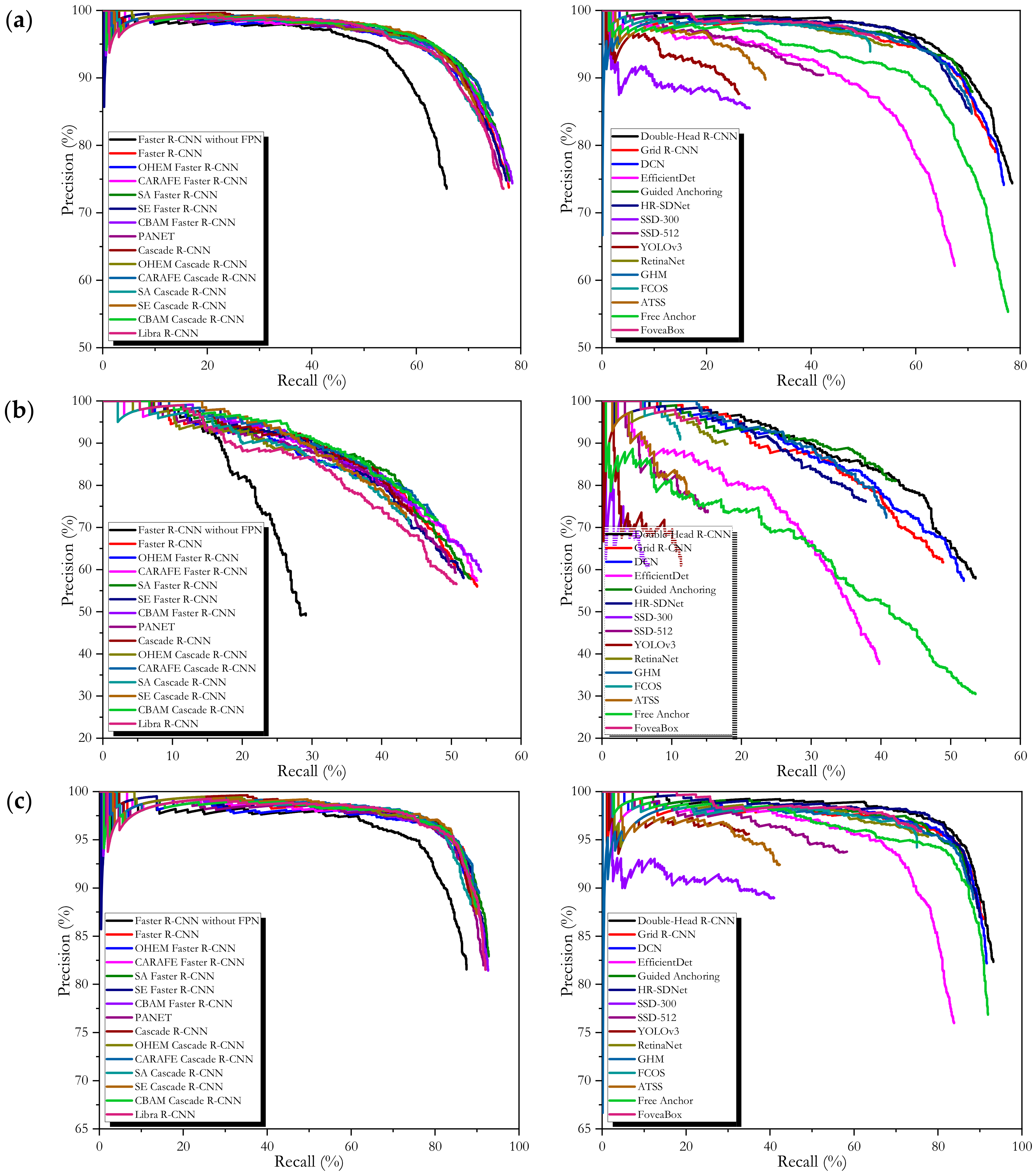
  • If using mAP as the accuracy criteria, among the 30 detectors, the best on the entire scenes is 75.74% of double-head R-CNN, that on the inshore scenes is 47.70% of CBAM Faster R-CNN, and that on the offshore scenes is 91.34% of Double-Head R-CNN. If using F1 as the accuracy criteria, the best on the entire scenes is 0.79 of CARAFE Cascade R-CNN and CBAM Faster R-CNN, that on the inshore scenes is 0.59 of Faster R-CNN, and that on the offshore scenes is 0.90 of CARAFE Cascade R-CNN and CBAM Faster R-CNN. If using Pd as the accuracy criteria, the best on the entire scenes is 78.47% of Double-Head R-CNN, that on the inshore scenes is 54.25% of CBAM Faster R-CNN, and that on the offshore scenes is 93.18% of Double-Head R-CNN.
  • There is a huge accuracy gap between the inshore scenes and the offshore ones, e.g., the inshore accuracy of Faster R-CNN is far inferior to the offshore one (46.76% mAP << 89.99% mAP and 0.59 F1 << 0.87 F1). This phenomenon is consistent with common sense, because ships in the inshore scenes are harder to detect than the offshore, due to the severe interference of land, harbor facilities, etc. Thus, one can use LS-SSDD-v1.0 to emphatically study the inshore ship detection.
  • On the entire dataset, the optimal accuracies are 75.74% mAP of Double-Head R-CNN, 0.79 F1 of CARAFE Cascade R-CNN and CBAM Faster R-CNN, and 78.47% Pd of Double-Head R-CNN. Therefore, there is still a huge research space for future scholars. However, so far, the existing four datasets have almost reached a satisfactory accuracy (about 90% mAP), e.g., for SSDD, the existing open reports [1,2,4,5,6,15] have reached >95% mAP. Thus, related scholars may have resistance in driving the emergence of more excellent research results. In particular, it needs to be clarified that the accuracies on LS-SSDD-v1.0 are universally lower that on the other datasets if using same detectors. This phenomenon is because small ship detection in large-scale space-borne SAR images is a challenging task, instead of the problem from our annotation process. In fact, the seven steps in Section 3 has been able to guarantee the authenticity of dataset annotation. In short, LS-SSDD-v1.0 can promote a new round of SAR ship detection research upsurge.
  • Last but not least, to facilitate the understanding of these 30 research baselines, we make a general analysis of them. (1) Faster R-CNN with FPN has a better accuracy than Faster R-CNN without FPN because FPN can improve detection performance of ships with different sizes. (2) OHEM Faster R-CNN has a worse accuracy than Faster R-CNN because OHEM can suppress false alarms but miss-detect many ships. (3) CARAFE Faster R-CNN has a similar accuracy to Faster R-CNN; probably, its up-sampling module is insensitive to small ships. (4) SA Faster R-CNN has a better accuracy than Faster R-CNN because space attention can capture more valuable information. (5) SE Faster R-CNN has a similar accuracy to Faster R-CNN; probably, its squeeze and excitation mechanism cannot respond small ships. (6) CBAM Faster R-CNN has a better accuracy than Faster R-CNN because its spatial and channel attention can promote information flow. (7) PANET has a worse accuracy than Faster R-CNN, probably its pyramid network losses much information of small ships due to excessive feature integration. (8) Cascade R-CNN has a worse accuracy than Faster R-CNN because its cascaded IOU threshold mechanism can improve the quality of boxes but miss-detect other ships. (9) Cascade R-CNN with other improvements have a similar change rule to Faster R-CNN with these improvements (10) Libra R-CNN has a worse accuracy than Faster R-CNN; probably, it has resistance in solving lots of negative samples leading to learning imbalance. (11) Double-Head R-CNN has a best accuracy because it has strong performance to distinguish ships and backgrounds, from its double head for classification and location. (12) Grid R-CNN has a worse accuracy than Faster R-CNN because its grid mechanism on the RPN network may not capture useful features from rather small ships. (13) DCN has a worse accuracy than Faster R-CNN because its deformed convolution kernel only captures larger receptive field that may miss small ships with small receptive field. (14) EfficientDet has a worse accuracy than Faster RCNN even Faster R-CNN without FPN, and one possible reason is that its pyramid network overemphasizes multi-scale information and leads to information loss of small ships. (15) Guided Anchoring has a worse accuracy than Faster R-CNN, probably because its anchor guidance mechanism can generate good suggestions of small ships. (16) HR-SDNet has a modest accuracy because its high-resolution backbone networks may not capture useful features of small ships which is not suitable low-resolution small ships. (17) SSD-300 and YOLOv3 have the worst accuracy than others, because they are not good at small ships. (18) SSD-512 has a better accuracy than SSD-300 because its input image size is bigger than SSD-300, so it can obtain more image information. (19) RetinaNet has a better accuracy than SSD-300, SSD-512, and YOLOv3 because its focal loss can address the imbalance between positive samples and negative ones. (20) GHM has a better accuracy than RetinaNet because its gradient harmonizing mechanism seems to be a hedging for the disharmonies. (21) FCOS has a worse accuracy than RetinaNet, and a possible reason is that its object detection in a per-pixel prediction fashion may be able to solve the low-solution SAR images. (22) ATSS has a bad accuracy, probably coming from its oscillation of loss function due to too much negative samples. (23) FreeAnchor has a better accuracy than other one-stage detectors because its anchor matching mechanism is similar to two-stage detectors. (24) FoveaBox has a modest accuracy but lower than RetinaNet because it directly learns the object existing possibility and the bounding box coordinates without anchor reference [118]. (25) Finally, the two-stage detectors (from No. 1 to No. 21) generally have better detection performance than one-stage ones (from No. 22 to No. 30) because two-stage detectors can achieve better region proposals.
Table 12 shows the detection speed and model information. In Table 12, the detectors of No. 1 to No. 21 are two-stage detectors, and the detectors of No. 22 to No. 30 are one-stage detectors. In general, the one-stage detectors have lighter network models than two-stage ones because they do not have heavy RPN networks. As a result, the detection speed of one-stage detectors is higher than two-stage ones. Moreover, in Table 12, if some improved modules or mechanism are added to the original detectors, e.g., Faster R-CNN and Cascade R-CNN, their models become bigger slightly, but these improvements do not necessarily lead to better detection performance, as shown in Table 9, Table 10, Table 11 and Table 12, the heaviest network model is from HR-SDNet (694 MB) but its detection accuracy is not the best, and the lightest network model is from SSD-300 (181 MB), leading to its worst detection accuracy. Finally, parameters and FLOPs have a positive proportion relationship.
Finally, we take faster R-CNN as an example to show its detection results in the 11.jpg in Figure 16. In Figure 16, the detection results are marked in blue and the corresponding ship ground truths are in Figure 8. Given limited pages, the detection results of other detectors are not shown any more.

7. Discussions

In this section, we will conduct experiments to confirm the effectiveness of PBHT-mechanism. Given limited pages, we merely select two two-stage detectors, i.e., Faster R-CNN and Cascade R-CNN, and two one-stage detectors, i.e., SSD-512 and RetinaNet, to perform such ablation studies.
Table 13 shows the detection performance comparison of PBHT-mechanism on the entire scenes, Table 14 shows the detection performance comparison of PBHT-mechanism on the inshore scenes, and Table 15 shows the detection performance comparison of PBHT-mechanism on the offshore scenes. Figure 17 shows the precision–recall curves with and without PBHT-mechanism.
From Table 13, Table 14 and Table 15, we can draw the following conclusions:
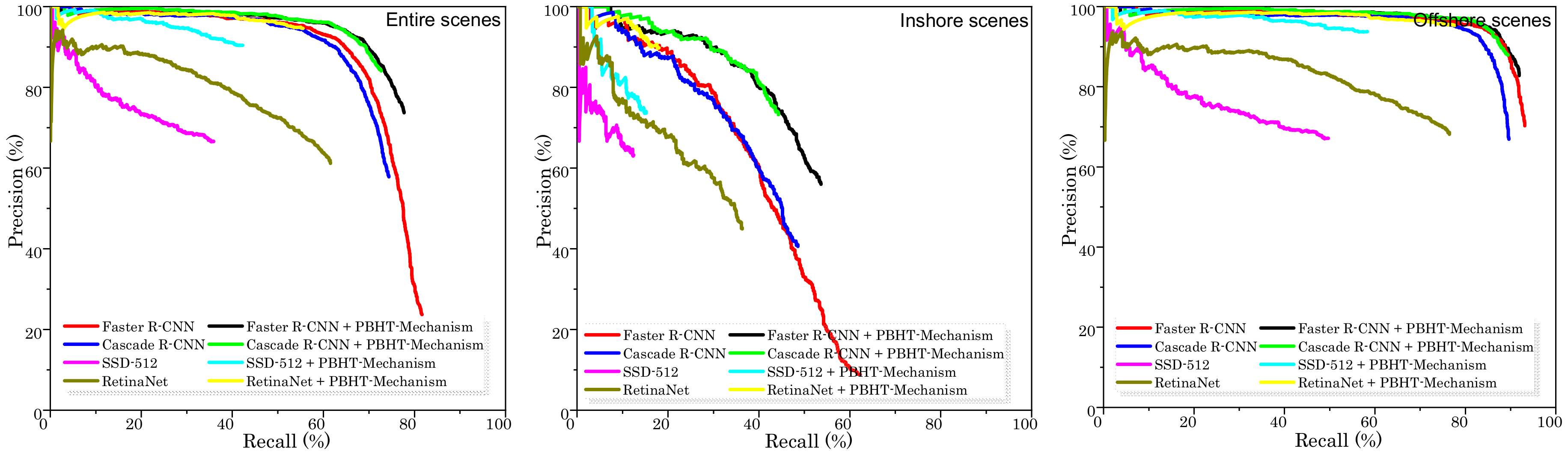
  • PBHT-mechanism can effectively suppress the false alarm probability Pf, i.e., (1) on the entire scenes, 26.26% Pf of Faster R-CNN with PBHT-mechanism << 76.27% Pf of Faster R-CNN without PBHT-Mechanism, 15.91% Pf of Cascade R-CNN with PBHT-mechanism << 42.15% Pf of Cascade R-CNN without PBHT-mechanism, 9.53% Pf of SSD-512 with PBHT-mechanism << 33.41% Pf of SSD-512 without PBHT-mechanism, and 5.38% Pf of RetinaNet with PBHT-mechanism << 38.80% Pf of RetinaNet without PBHT-mechanism; (2) on the inshore scenes, 44.04% Pf of Faster R-CNN with PBHT-mechanism << 91.13% Pf of Faster R-CNN without PBHT-mechanism, 26.78% Pf of Cascade R-CNN with PBHT-mechanism << 59.38% Pf of Cascade R-CNN without PBHT-mechanism, 26.37% Pf of SSD-512 with PBHT-mechanism << 36.78% Pf of SSD-512 without PBHT-mechanism and 10.17% Pf of RetinaNet with PBHT-mechanism << 55.04% Pf of RetinaNet without PBHT-mechanism; (3) on the offshore scenes, 17.18% Pf of Faster R-CNN with PBHT-mechanism << 29.73% Pf of Faster R-CNN without PBHT-mechanism, 12.10% Pf of Cascade R-CNN with PBHT-mechanism << 33.07% Pf of Cascade R-CNN without PBHT-mechanism, 6.24% Pf of SSD-512 with PBHT-mechanism << 32.88% Pf of SSD-512 without PBHT-mechanism, and 4.68% Pf of RetinaNet with PBHT-mechanism << 31.88% Pf of RetinaNet without PBHT-mechanism.
  • If using PBHT-mechanism, the detection probability Pd has a slight drop for some detectors. We hold the view that it is worth sacrificing a slight detection probability for a huge false alarm probability reduction, because the final good balance between Pf and Pd can be achieved. In other words, finally, mAP and F1, which simultaneously consider Pf and Pd, are obviously improved.
Figure 18 shows the detection result comparison of faster R-CNN with PBHT-mechanism and without PBHT-mechanism. In Figure 18a, if not using PBHT-mechanism, there are many false alarms of strong scattering bright spots occurring in the pure background areas (marked in magenta), and their classification scores are also relatively high although the score threshold is set as 0.5. Obviously, these false alarms are not likely to happen for traditional methods after sea-land segmentation. On the contrary, if using PBHT-mechanism, it is obvious that the above false alarms are all suppressed in pure backgrounds (all magenta boxes are removed), because models have learned the features of area without ships so as to discriminate real ships and brightened dots of land. Finally, we also realize that it is time-consuming for training to add many pure backgrounds samples (35 min/epoch >> 5 min/epoch), but we hold the view that it is cost-effective to achieve better detection performance because such practice does not slow down the final detection speed for the test or inference process.

8. Conclusions

This paper releases LS-SSDD-v1.0 for small ship detection from Sentinel-1 with large-scale backgrounds to meet the practical migration application of ship detection in large-scene space-borne SAR images in engineering. LS-SSDD-v1.0 has five advantages: (1) large-scale backgrounds, (2) small ship detection, (3) abundant pure backgrounds, (4) fully automatic detection flow, and (5) numerous and standardized research baselines. We introduce the establishment process and describe the five advantages in detail. Then, 30 research baselines are provided for scholars to facilitate future studies. Finally, based on abundant pure backgrounds, we also propose PBHT-mechanism to suppress false alarms of land and the experimental results verify its effectiveness. LS-SSDD-v1.0 is a challenging dataset because small ship detection in the practical large-scale space-borne SAR images in engineering migration applications is a challenging task. More importantly, LS-SSDD-v1.0 is also a dataset in line with the practical engineering migration applications in large-scale space-borne SAR images, exciting related scholars to research SAR ship detection methods with more engineering application value in the future, beneficial for the progress of SAR intelligent interpretation technology.
Our future work is as follows:
  • We will update LS-SSDD-v1.0 into v2.0 or higher, e.g., expanding the sample number, adding more typical scenarios, providing preferable research baselines, etc., in the future.
  • We will study more SAR ship detection methods based on LS-SSDD-v1.0, e.g., further improving the accuracy of the state-of-the-art, further enhancing the accuracy of inshore ships, etc.
  • We will combine deep learning abstract features and traditional concrete ones to further improve accuracy (e.g., Ai et al. [125]). So far, most scholars in this SAR ship detection community still scarcely focus on much information of SAR images and ship identification, when they applied those object detectors in the deep learning filed to this SAR ship detection field.

Author Contributions

Conceptualization, T.Z.; Methodology, T.Z.; Software, X.K.; Validation, X.Z. (Xu Zhan); Formal analysis, D.P.; Investigation, D.K.; Resources, J.L.; Data Curation, S.W.; Writing—original draft preparation, T.Z.; Writing—review and editing, X.Z. (Xiaoling Zhang); Visualization, H.S.; Supervision, J.S.; Project Administration, Y.Z.; Funding acquisition, X.Z. (Xiaoling Zhang). All authors have read and agreed to the published version of the manuscript.

Funding

This research was funded in part by the National Natural Science Foundation of China (61571099, 61501098 and 61671113), and in part by the National Key R&D Program of China (2017YFB0502700).

Acknowledgments

We thank anonymous reviewers for their comments towards improving this manuscript. The authors would also like to thank European Space Agency (ESA) for providing Sentinel-1 SAR images.

Conflicts of Interest

The authors declare no conflict of interest.

References

  1. Zhang, T.; Zhang, X.; Shi, J.; Wei, S. HyperLi-Net: A hyper-light deep learning network for high-accurate and high-speed ship detection from synthetic aperture radar imagery. ISPRS J. Photogramm. Remote Sens. 2020, 167, 123–153. [Google Scholar] [CrossRef]
  2. Zhang, T.; Zhang, X. ShipDeNet-20: An only 20 convolution layers and <1-MB lightweight SAR ship detector. IEEE Geosci. Remote Sens. Lett. 2020. [Google Scholar] [CrossRef]
  3. Zhang, T.; Zhang, X. High-speed ship detection in SAR images based on a grid convolutional neural network. Remote Sens. 2019, 10, 1206. [Google Scholar] [CrossRef] [Green Version]
  4. Zhang, T.; Zhang, X.; Shi, J.; Wei, S. Depthwise separable convolution neural network for high-speed SAR ship detection. Remote Sens. 2019, 11, 2483. [Google Scholar] [CrossRef] [Green Version]
  5. Zhang, X.; Zhang, T.; Shi, J.; Wei, S. High-speed and high-accurate SAR ship detection based on a depthwise separable convolution neural network. J. Radars 2019, 8, 841–851. [Google Scholar]
  6. Wei, S.; Su, H.; Ming, J.; Wang, C.; Yan, M.; Kumar, D.; Shi, J.; Zhang, X. Precise and robust ship detection for high-resolution SAR imagery based on HR-SDNet. Remote Sens. 2020, 12, 167. [Google Scholar] [CrossRef] [Green Version]
  7. Wei, S.; Zeng, X.; Qu, Q.; Wang, M.; Su, H.; Shi, J. HRSID: A high-resolution SAR images dataset for ship detection and instance segmentation. IEEE Access 2020, 8, 120234–120254. [Google Scholar] [CrossRef]
  8. Chang, Y.-L.; Anagaw, A.; Chang, L.; Wang, Y.C.; Hsiao, C.-Y.; Lee, W.-H. Ship detection based on YOLOv2 for SAR imagery. Remote Sens. 2019, 11, 786. [Google Scholar] [CrossRef] [Green Version]
  9. Pelich, R.; Chini, M.; Hostache, R.; Matgen, P.; Lopez-Martinez, C.; Nuevo, M.; Ries, P.; Eiden, G. Large-scale automatic vessel monitoring based on dual-polarization Sentinel-1 and AIS data. Remote Sens. 2019, 11, 1078. [Google Scholar] [CrossRef] [Green Version]
  10. Wang, Y.; Wang, C.; Zhang, H.; Dong, Y.; Wei, S. A SAR dataset of ship detection for deep learning under complex backgrounds. Remote Sens. 2019, 11, 765. [Google Scholar] [CrossRef] [Green Version]
  11. Chen, S.; Zhang, J.; Zhan, R. R2FA-Det: Delving into high-quality rotatable boxes for ship detection in SAR images. Remote Sens. 2020, 12, 2031. [Google Scholar] [CrossRef]
  12. Li, J.; Qu, C.; Shao, J. Ship detection in SAR images based on an improved Faster R-CNN. In Proceedings of the 2017 SAR in Big Data Era: Models, Methods and Applications (BIGSARDATA), Beijing, China, 13–14 November 2017; pp. 1–6. [Google Scholar]
  13. Cui, Z.; Li, Q.; Cao, Z.; Liu, N. Dense attention pyramid networks for multi-scale ship detection in SAR images. IEEE Trans. Geosci. Remote Sens. 2019, 57, 8983–8997. [Google Scholar] [CrossRef]
  14. Cui, Z.; Wang, X.; Liu, N.; Cao, Z.; Yang, J. Ship detection in large-scale SAR images via spatial shuffle-group enhance attention. IEEE Trans. Geosci. Remote Sens. 2020. [Google Scholar] [CrossRef]
  15. Zhao, Y.; Zhao, L.; Xiong, B.; Kuang, G. Attention receptive pyramid network for ship detection in SAR images. IEEE J. Sel. Topics Appl. Earth Observ. Remote Sens. 2020, 13, 2738–2756. [Google Scholar] [CrossRef]
  16. Lin, Z.; Ji, K.; Leng, X.; Kuang, G. Squeeze and excitation rank Faster R-CNN for ship detection in SAR images. IEEE Geosci. Remote Sens. Lett. 2019, 16, 751–755. [Google Scholar] [CrossRef]
  17. Deng, Z.; Sun, H.; Zhou, S.; Zhao, J.; Lei, L.; Zou, H. Multi-scale object detection in remote sensing imagery with convolutional neural networks. ISPRS J. Photogramm. Remote Sens. 2018, 145, 3–22. [Google Scholar] [CrossRef]
  18. Deng, Z.; Sun, H.; Zhou, S.; Zhao, J. Learning deep ship detector in SAR images from scratch. IEEE Trans. Geosci. Remote Sens. 2019, 57, 4021–4039. [Google Scholar] [CrossRef]
  19. Zhao, J.; Guo, W.; Zhang, Z.; Yu, W. A coupled convolutional neural network for small and densely clustered ship detection in SAR images. Sci. China Inf. Sci. 2018, 62, 42301. [Google Scholar] [CrossRef] [Green Version]
  20. Zhao, J.; Zhang, Z.; Yu, W.; Truong, T.-K. A cascade coupled convolutional neural network guided visual attention method for ship detection from SAR images. IEEE Access 2018, 6, 50693–50708. [Google Scholar] [CrossRef]
  21. Jiao, J.; Zhang, Y.; Sun, H.; Yang, X.; Gao, X.; Hong, W.; Fu, K.; Sun, X. A densely connected end-to-end neural network for multiscale and multiscene SAR ship detection. IEEE Access 2018, 6, 20881–20892. [Google Scholar] [CrossRef]
  22. Sun, X.; Wang, Z.; Sun, Y.; Diao, W.; Zhang, Y.; Fu, K. AIR-SARShip-1.0: High-resolution SAR ship detection dataset. J. Radars 2019, 8, 852–862. [Google Scholar]
  23. Fan, W.; Zhou, F.; Bai, X.; Tao, M.; Tian, T. Ship detection using deep convolutional neural networks for PolSAR images. Remote Sens. 2019, 11, 2862. [Google Scholar] [CrossRef] [Green Version]
  24. Jin, K.; Chen, Y.; Xu, B.; Yin, J.; Wang, X.; Yang, J. A patch-to-pixel convolutional neural network for small ship detection with PolSAR Images. IEEE Trans. Geosci. Remote Sens. 2020, 58, 6623–6638. [Google Scholar] [CrossRef]
  25. Song, J.; Kim, D.-J.; Kang, K.-M. Automated procurement of training data for machine learning algorithm on ship detection using AIS information. Remote Sens. 2020, 12, 1443. [Google Scholar] [CrossRef]
  26. Gao, F.; Shi, W.; Wang, J.; Yang, E.; Zhou, H. Enhanced feature extraction for ship detection from multi-resolution and multi-scene synthetic aperture radar (SAR) images. Remote Sens. 2019, 11, 2694. [Google Scholar] [CrossRef] [Green Version]
  27. Gao, F.; Shi, W.; Wang, J.; Hussain, A.; Zhou, H. Anchor-free Convolutional Network with Dense Attention Feature Aggregation for Ship Detection in SAR Images. Remote Sens. 2020, 12, 2619. [Google Scholar] [CrossRef]
  28. An, Q.; Pan, Z.; You, H. Ship detection in Gaofen-3 SAR images based on sea clutter distribution analysis and deep convolutional neural network. Sensors 2018, 18, 334. [Google Scholar] [CrossRef] [Green Version]
  29. An, Q.; Pan, Z.; Liu, L.; You, H. DRBox-v2: An improved detector with rotatable boxes for target detection in SAR images. IEEE Trans. Geosci. Remote Sens. 2019, 57, 8333–8349. [Google Scholar] [CrossRef]
  30. Yang, R.; Wang, G.; Pan, Z.; Lu, H.; Zhang, H.; Jia, X. A novel false alarm suppression method for CNN-based SAR ship detector. IEEE Geosci. Remote Sens. Lett. 2020. [Google Scholar] [CrossRef]
  31. Chen, C.; He, C.; Hu, C.; Pei, H.; Jiao, L. MSARN: A deep neural network based on an adaptive recalibration mechanism for multiscale and arbitrary-oriented SAR ship detection. IEEE Access 2019, 7, 159262–159283. [Google Scholar] [CrossRef]
  32. Zhang, X.; Wang, H.; Xu, C.; Lv, Y.; Fu, C.; Xiao, H.; He, Y. A lightweight feature optimizing network for ship detection in SAR image. IEEE Access 2019, 7, 141662–141678. [Google Scholar] [CrossRef]
  33. Fan, Q.; Chen, F.; Cheng, M.; Lou, S.; Xiao, R.; Zhang, B.; Wang, C.; Li, J. Ship detection using a fully convolutional network with compact polarimetric SAR images. Remote Sens. 2019, 11, 2171. [Google Scholar] [CrossRef] [Green Version]
  34. Mao, Y.; Yang, Y.; Ma, Z.; Li, M.; Su, H.; Zhang, J. Efficient low-cost ship detection for SAR imagery based on simplified U-Net. IEEE Access 2020, 8, 69742–69753. [Google Scholar] [CrossRef]
  35. Fu, J.; Sun, X.; Wang, Z.; Fu, K. An anchor-free method based on feature balancing and refinement network for multiscale ship detection in SAR images. IEEE Trans. Geosci. Remote Sens. 2020. [Google Scholar] [CrossRef]
  36. Eldhuset, K. An automatic ship and ship wake detection system for space-borne SAR images in coastal regions. IEEE Trans. Geosci. Remote Sens. 1996, 34, 1010–1019. [Google Scholar] [CrossRef]
  37. Lin, I.I.; Keong, K.L.; Yuan-Chung, L.; Khoo, V. Ship and ship wake detection in the ERS SAR imagery using computer-based algorithm. In Proceedings of the 1997 IEEE International Geoscience and Remote Sensing Symposium Proceedings. Remote Sensing—A Scientific Vision for Sustainable Development, Singapore, 3–8 August 1997; pp. 151–153. [Google Scholar]
  38. Renga, A.; Graziano, M.D.; Moccia, A. Segmentation of marine SAR images by sublook analysis and application to sea traffic monitoring. IEEE Trans. Geosci. Remote Sens. 2019, 57, 1463–1477. [Google Scholar] [CrossRef]
  39. Ai, J.; Qi, X.; Yu, W.; Deng, Y.; Liu, F.; Shi, L. A new CFAR ship detection algorithm based on 2-D joint log-normal distribution in SAR images. IEEE Geosci. Remote Sens. Lett. 2010, 7, 806–810. [Google Scholar] [CrossRef]
  40. Ai, J.; Yang, X.; Song, J.; Dong, Z.; Jia, L.; Zhou, F. An adaptively truncated clutter-statistics-based two-parameter CFAR detector in SAR imagery. IEEE J. Ocean. Eng. 2018, 43, 267–279. [Google Scholar] [CrossRef]
  41. Ai, J.; Luo, Q.; Yang, X.; Yin, Z.; Xu, H. Outliers-robust CFAR detector of gaussian clutter based on the truncated-maximum-likelihood-estimator in SAR imagery. IEEE Trans. Intell. Transp. Syst. 2020, 21, 2039–2049. [Google Scholar] [CrossRef]
  42. Brizi, M.; Lombardo, P.; Pastina, D. Exploiting the shadow information to increase the target detection performance in SAR images. In Proceedings of the 5th international conference and exhibition on radar systems, Brest, France, 17–21 May 1999. [Google Scholar]
  43. Iervolino, P.; Guida, R. A novel ship detector based on the generalized-likelihood ratio test for SAR imagery. IEEE J. Sel. Topics Appl. Earth Observ. Remote Sens. 2017, 10, 3616–3630. [Google Scholar] [CrossRef] [Green Version]
  44. Sciotti, M.; Pastina, D.; Lombardo, P. Exploiting the polarimetric information for the detection of ship targets in non-homogeneous SAR images. In Proceedings of the IEEE International Geoscience and Remote Sensing Symposium, Toronto, ON, Canada, 24–28 June 2002; pp. 1911–1913. [Google Scholar]
  45. Tello, M.; Lopez-Martinez, C.; Mallorqui, J.J. A novel algorithm for ship detection in SAR imagery based on the wavelet transform. IEEE Geosci. Remote Sens. Lett. 2005, 2, 201–205. [Google Scholar] [CrossRef]
  46. Schwegmann, C.P.; Kleynhans, W.; Salmon, B.P. Synthetic aperture radar ship detection using Haar-like features. IEEE Geosci. Remote Sens. Lett. 2017, 14, 154–158. [Google Scholar] [CrossRef] [Green Version]
  47. Marino, A.; Sanjuan-Ferrer, M.J.; Hajnsek, I.; Ouchi, K. Ship detection with spectral analysis of synthetic aperture radar: A comparison of new and well-known algorithms. Remote Sens. 2015, 7, 5416–5439. [Google Scholar] [CrossRef]
  48. Xie, T.; Zhang, W.; Yang, L.; Wang, Q.; Huang, J.; Yuan, N. Inshore ship detection based on level set method and visual saliency for SAR images. Sensors 2018, 18, 3877. [Google Scholar] [CrossRef] [PubMed] [Green Version]
  49. Zhai, L.; Li, Y.; Su, Y. Inshore ship detection via saliency and context information in high-resolution SAR Images. IEEE Geosci. Remote Sens. Lett. 2016, 13, 1870–1874. [Google Scholar] [CrossRef]
  50. Cui, X.; Su, Y.; Chen, S. A saliency detector for polarimetric SAR ship detection using similarity test. IEEE J. Sel. Top. Appl. Earth Observ. Remote Sens. 2019, 12, 3423–3433. [Google Scholar] [CrossRef]
  51. Wang, X.; Li, G.; Zhang, X.P.; He, Y. Ship detection in SAR images via local contrast of fisher vectors. IEEE Trans. Geosci. Remote Sens. 2020, 58, 6467–6479. [Google Scholar] [CrossRef]
  52. Wang, X.; Chen, C.; Pan, Z.; Pan, Z. Superpixel-based LCM detector for faint ships hidden in strong noise background SAR imagery. IEEE Geosci. Remote Sens. Lett. 2019, 16, 417–421. [Google Scholar] [CrossRef]
  53. Lin, H.; Chen, H.; Jin, K.; Zeng, L.; Yang, J. Ship detection with superpixel-level fisher vector in high-resolution SAR images. IEEE Geosci. Remote Sens. Lett. 2020, 17, 247–251. [Google Scholar] [CrossRef]
  54. Tings, B.; Pleskachevsky, A.; Velotto, D.; Jacobsen, S. Extension of ship wake detectability model for non-linear influences of parameters using satellite-based X-band synthetic aperture radar. Remote Sens. 2019, 11, 563. [Google Scholar] [CrossRef] [Green Version]
  55. Biondi, F. A polarimetric extension of low-rank plus sparse decomposition and radon transform for ship wake detection in synthetic aperture radar images. IEEE Geosci. Remote Sens. Lett. 2019, 16, 75–79. [Google Scholar] [CrossRef]
  56. Karakuş, O.; Rizaev, I.; Achim, A. Ship Wake Detection in SAR Images via Sparse Regularization. IEEE Trans. Geosci. Remote Sens. 2020, 58, 1665–1677. [Google Scholar] [CrossRef] [Green Version]
  57. Cao, C.; Zhang, J.; Meng, J.; Zhang, X.; Mao, X. Analysis of ship detection performance with full-, compact- and dual-polarimetric SAR. Remote Sens. 2019, 11, 18. [Google Scholar] [CrossRef] [Green Version]
  58. Hwang, J.-I.; Jung, H.-S. Automatic Ship detection using the artificial neural network and support vector machine from X-band SAR satellite images. Remote Sens. 2018, 10, 1799. [Google Scholar] [CrossRef] [Green Version]
  59. Guo, R.; Cui, J.; Jing, G.; Zhang, S.; Xing, M. Validating GEV model for reflection symmetry-based ocean ship detection with Gaofen-3 dual-polarimetric data. Remote Sens. 2020, 12, 1148. [Google Scholar] [CrossRef] [Green Version]
  60. Liang, Y.; Sun, K.; Zeng, Y.; Li, G.; Xing, M. An adaptive hierarchical detection method for ship targets in high-resolution SAR images. Remote Sens. 2020, 12, 303. [Google Scholar] [CrossRef] [Green Version]
  61. Wang, J.; Zheng, T.; Lei, P.; Bai, X. A hierarchical convolution neural network (CNN)-based ship target detection method in space-borne SAR imagery. Remote Sens. 2019, 11, 620. [Google Scholar] [CrossRef] [Green Version]
  62. Ma, M.; Chen, J.; Liu, W.; Yang, W. Ship classification and detection based on CNN using GF-3 SAR images. Remote Sens. 2018, 10, 2043. [Google Scholar] [CrossRef] [Green Version]
  63. Marino, A.; Hajnsek, I. Ship detection with TanDEM-X data extending the polarimetric notch filter. IEEE Geosci. Remote Sens. Lett. 2015, 12, 2160–2164. [Google Scholar] [CrossRef] [Green Version]
  64. Zhang, T.; Marino, A.; Xiong, H.; Yu, W. A ship detector applying principal component analysis to the polarimetric notch filter. Remote Sens. 2018, 10, 948. [Google Scholar] [CrossRef] [Green Version]
  65. Dechesne, C.; Lefèvre, S.; Vadaine, R.; Hajduch, G.; Fablet, R. Ship identification and characterization in Sentinel-1 SAR images with multi-task deep learning. Remote Sens. 2019, 11, 2997. [Google Scholar] [CrossRef] [Green Version]
  66. Liu, G.; Zhang, X.; Meng, J. A small ship target detection method based on polarimetric SAR. Remote Sens. 2019, 11, 2938. [Google Scholar] [CrossRef] [Green Version]
  67. Greidanus, H.; Alvarez, M.; Santamaria, C.; Thoorens, F.; Kourti, N.; Argentieri, P. The SUMO ship detector algorithm for satellite radar images. Remote Sens. 2017, 9, 246. [Google Scholar] [CrossRef] [Green Version]
  68. Joshi, S.K.; Baumgartner, S.; Silva, A.; Krieger, G. Range-doppler based CFAR ship detection with automatic training data selection. Remote Sens. 2019, 11, 1270. [Google Scholar] [CrossRef] [Green Version]
  69. Zhang, Y.; Xiong, W.; Dong, X.; Hu, C.; Sun, Y. GRFT-based moving ship target detection and imaging in geosynchronous SAR. Remote Sens. 2018, 10, 2002. [Google Scholar] [CrossRef] [Green Version]
  70. Kang, M.; Ji, K.; Leng, X.; Lin, Z. Contextual region-based convolutional neural network with multilayer fusion for SAR ship detection. Remote Sens. 2017, 9, 860. [Google Scholar] [CrossRef] [Green Version]
  71. LeCun, Y.; Bengio, Y.; Hinton, G. Deep learning. Nature 2015, 521, 436–444. [Google Scholar] [CrossRef] [PubMed]
  72. Liu, Y.; Zhang, M.; Xu, P.; Guo, Z. SAR ship detection using sea-land segmentation-based convolutional neural network. In Proceedings of the International Workshop on Remote Sensing with Intelligent Processing (RSIP), Shanghai, China, 18–21 May 2017; pp. 1–4. [Google Scholar]
  73. Sentinel Online. Available online: https://sentinel.esa.int/web/sentinel/ (accessed on 15 July 2020).
  74. Lin, T.-Y.; Maire, M.; Belongie, S.; Hays, J.; Perona, P.; Ramanan, D.; Doll´ar, P.; Zitnick, C. Microsoft COCO: Common objects in context. arXiv 2014, arXiv:1405.0312. [Google Scholar]
  75. Ren, S.; He, K.; Girshick, R.; Sun, J. Faster R-CNN: Towards real-time object detection with region proposal networks. IEEE Trans. Pattern Anal. Mach. Intell. 2017, 39, 1137–1149. [Google Scholar] [CrossRef] [Green Version]
  76. Liu, W.; Anguelov, D.; Erhan, D.; Szegedy, C.; Reed, S.; Fu, C.; Berg, A. SSD: Single shot multibox detector. In Proceedings of the 14th European Conference on Computer Vision, Amsterdam, The Netherlands, 11–14 October 2016; pp. 21–37. [Google Scholar]
  77. Lin, T.Y.; Goyal, P.; Girshick, R.; He, K.; Dollár, P. Focal loss for dense object detection. In Proceedings of the International Conference on Computer Vision, Venice, Italy, 22–29 October 2017; pp. 2999–3007. [Google Scholar]
  78. Cai, Z.; Vasconcelos, N. Cascade R-CNN: Delving into high quality object detection. arXiv 2017, arXiv:1712.00726. [Google Scholar]
  79. Everingham, M.; Van Gool, L.; Williams, C.K.; Winn, J.; Zisserman, A. The PASCAL visual object classes (VOC) challenge. Int. J. Comput. Vis. 2010, 88, 303–338. [Google Scholar] [CrossRef] [Green Version]
  80. Huang, L.; Liu, B.; Li, B.; Guo, W.; Yu, W.; Zhang, Z.; Yu, W. OpenSARShip: A dataset dedicated to Sentinel-1 ship interpretation. IEEE J. Sel. Topics Appl. Earth Observ. Remote Sens. 2018, 11, 195–208. [Google Scholar] [CrossRef]
  81. Hou, X.; Ao, W.; Song, Q.; Lai, J.; Wang, H.; Xu, F. FUSAR-Ship: Building a high-resolution SAR-AIS matchup dataset of Gaofen-3 for ship detection and recognition. Sci. China Inf. Sci. 2020, 63, 140303. [Google Scholar] [CrossRef] [Green Version]
  82. Copernicus Open Access Hub. Available online: https://scihub.copernicus.eu/ (accessed on 15 July 2020).
  83. Torres, R.; Snoeij, P.; Geudtner, D.; Bibby, D.; Davidson, M.; Attema, E.; Potin, P.; Rommen, B.; Floury, N.; Brown, M.; et al. GMES Sentinel-1 mission. Remote Sens. Environ. 2012, 120, 9–24. [Google Scholar] [CrossRef]
  84. Leng, X.; Ji, K.; Zhou, S.; Xing, X.; Zou, H. Discriminating ship from radio frequency interference based on noncircularity and non-gaussianity in Sentinel-1 SAR imagery. IEEE Trans. Geosci. Remote Sens 2019, 57, 352–363. [Google Scholar] [CrossRef]
  85. Sentinel-1 Toolbox. Available online: https://sentinels.copernicus.eu/web/ (accessed on 15 July 2020).
  86. GDAL Documentation Edit on GitHub. Available online: https://gdal.org/ (accessed on 15 July 2020).
  87. Xiao, F.; Ligteringen, H.; Gulijk, C.; Ale, B. Comparison study on AIS data of ship traffic behavior. Ocean Eng. 2015, 95, 84–93. [Google Scholar] [CrossRef] [Green Version]
  88. IMO. Available online: http://www.imo.org/ (accessed on 15 July 2020).
  89. World Glacier Inventory. Available online: http://nsidc.org/data/glacier_inventory/ (accessed on 15 July 2020).
  90. Bentes, C.; Frost, A.; Velotto, D.; Tings, B. Ship-Iceberg Discrimination with Convolutional Neural Networks in High Resolution SAR Images. In Proceedings of the 11th European Conference on Synthetic Aperture Radar, Hamburg, Germany, 6–9 June 2016; pp. 1–4. [Google Scholar]
  91. World Meteorological Organization. Available online: https://worldweather.wmo.int/en/home.html (accessed on 15 July 2020).
  92. Park, J.; Lee, J.; Seto, K.; Hochberg, T.; Wong, B.A.; Miller, N.A.; Takasaki, K.; Kubota, H.; Oozeki, Y.; Doshi, S.; et al. Illuminating dark fishing fleets in North Korea. Sci. Adv. 2020, 6, eabb1197. [Google Scholar] [CrossRef]
  93. Wang, J.; Lu, C.; Jiang, W. Simultaneous Ship Detection and Orientation Estimation in SAR Images Based on Attention Module and Angle Regression. Sensors 2018, 18, 2851. [Google Scholar] [CrossRef] [Green Version]
  94. Liu, C.; Yang, J.; Yin, J.; An, W. Coastline detection in SAR images using a hierarchical level set segmentation. IEEE J. Sel. Topics Appl. Earth Observ. Remote Sens. 2016, 9, 4908–4920. [Google Scholar] [CrossRef]
  95. Modava, M.; Akbarizadeh, G.; Soroosh, M. Hierarchical coastline detection in SAR images based on spectral-textural features and global–local information. IET Radar Sonar Navig. 2019, 13, 2183–2195. [Google Scholar] [CrossRef]
  96. Modava, M.; Akbarizadeh, G.; Soroosh, M. Integration of Spectral Histogram and Level Set for Coastline Detection in SAR Images. IEEE Trans. Aerosp. Electron. Syst. 2019, 55, 810–819. [Google Scholar] [CrossRef]
  97. Chen, K.; Wang, J.; Pang, J.; Cao, Y.; Xiong, Y.; Li, X.; Sun, S.; Feng, W.; Liu, Z.; Xu, J.; et al. MMDetection: Open MMLab detection toolbox and benchmark. arXiv 2019, arXiv:1906.07155. [Google Scholar]
  98. Sergios, T. Stochastic gradient descent. Mach. Learn. 2015, 161–231. [Google Scholar] [CrossRef]
  99. Goyal, P.; Dollár, P.; Girshick, R.; Noordhuis, P.; Wesolowski, L.; Kyrola, A.; Tulloch, A.; Jia, Y.; He, K. Accurate, Large Minibatch SGD: Training ImageNet in 1 h. arXiv 2017, arXiv:1706.02677. [Google Scholar]
  100. Lin, T.-Y.; Doll´ar, P.; Girshick, R.; He, K.; Hariharan, B.; Belongie, S. Feature pyramid networks for object detection. arXiv 2016, arXiv:1612.03144. [Google Scholar]
  101. Shrivastava, A.; Gupta, A.; Girshick, R. Training region-based object detectors with online hard example mining. In Proceedings of the 2016 IEEE Conference on Computer Vision and Pattern Recognition (CVPR), Las Vegas, NV, USA, 27–30 June 2016; pp. 761–769. [Google Scholar]
  102. Wang, J.; Chen, K.; Xu, R.; Change Loy, C.; Lin, D. CARAFE: Content-aware reassembly of features. arXiv 2019, arXiv:1905.02188. [Google Scholar]
  103. Zhu, X.; Cheng, D.; Zhang, Z.; Lin, S.; Dai, J. An empirical study of spatial attention mechanisms in deep networks. In Proceedings of the 2019 IEEE/CVF International Conference on Computer Vision (ICCV), Seoul, Korea, 27 October–2 November 2019; pp. 6687–6696. [Google Scholar]
  104. Hu, J.; Shen, L.; Sun, G. Squeeze-and-Excitation Networks. arXiv 2017, arXiv:1709.01507. [Google Scholar]
  105. Woo, S.; Park, J.; Lee, J.; So Kweon, I. CBAM: Convolutional block attention module. arXiv 2018, arXiv:1807.06521. [Google Scholar]
  106. Liu, S.; Qi, L.; Qin, H.; Shi, J.; Jia, J. Path aggregation network for instance segmentation. arXiv 2018, arXiv:1803.01534. [Google Scholar]
  107. Pang, J.; Chen, K.; Shi, J.; Feng, H.; Ouyang, W.; Lin, D. Libra R-CNN: Towards balanced learning for object detection. arXiv 2019, arXiv:1904.02701. [Google Scholar]
  108. Wu, Y.; Chen, Y.; Yuan, L.; Liu, Z.; Wang, L.; Li, H.; Fu, Y. Rethinking classification and localization for object detection. arXiv 2019, arXiv:1904.06493. [Google Scholar]
  109. Lu, X.; Li, B.; Yue, Y.; Li, Q.; Yan, J. Grid R-CNN. In Proceedings of the 2019 IEEE/CVF Conference on Computer Vision and Pattern Recognition (CVPR), Long Beach, CA, USA, 15–20 June 2019; pp. 7355–7364. [Google Scholar]
  110. Dai, J.; Qi, H.; Xiong, Y.; Li, Y.; Zhang, G.; Hu, H.; Wei, Y. Deformable convolutional networks. In Proceedings of the 2017 IEEE International Conference on Computer Vision (ICCV), Venice, Italy, 22–29 October 2017; pp. 764–773. [Google Scholar]
  111. Tan, M.; Pang, R.; Le, Q.V. EfficientDet: Scalable and efficient object detection. arXiv 2019, arXiv:1911.09070. [Google Scholar]
  112. Wang, J.; Chen, K.; Yang, S.; Change Loy, C.; Lin, D. Region proposal by guided anchoring. arXiv 2019, arXiv:1901.03278. [Google Scholar]
  113. Redmon, J.; Farhadi, A. YOLOv3: An incremental improvement. arXiv 2018, arXiv:1804.02767. [Google Scholar]
  114. Li, B.; Liu, Y.; Wang, X. Gradient harmonized single-stage detector. arXiv 2018, arXiv:1811.05181. [Google Scholar] [CrossRef]
  115. Tian, Z.; Shen, C.; Chen, H.; He, T. FCOS: Fully convolutional one-stage object detection. arXiv 2019, arXiv:1904.01355. [Google Scholar]
  116. Zhang, S.; Chi, C.; Yao, Y.; Lei, Z.; Li, S.Z. Bridging the gap between anchor-based and anchor-free detection via adaptive training sample selection. arXiv 2019, arXiv:1912.02424. [Google Scholar]
  117. Zhang, X.; Wan, F.; Liu, C.; Ye, Q. FreeAnchor: Learning to match anchors for visual object detection. arXiv 2019, arXiv:1909.02466. [Google Scholar]
  118. Kong, T.; Sun, F.; Liu, H.; Jiang, Y.; Li, L.; Shi, J. FoveaBox: Beyond anchor-based object detector. arXiv 2019, arXiv:1904.03797. [Google Scholar]
  119. He, K.; Zhang, X.; Ren, S.; Sun, J. Deep residual learning for image recognition. arXiv 2015, arXiv:1512.03385. [Google Scholar]
  120. Simonyan, K.; Zisserman, A. Very deep convolutional networks for large-scale image recognition. arXiv 2014, arXiv:1409.1556. [Google Scholar]
  121. He, K.; Girshick, R.; Doll´ar, P. Rethinking ImageNet pre-training. arXiv 2018, arXiv:1811.08883. [Google Scholar]
  122. Hosang, J.; Benenson, R.; Schiele, B. Learning non-maximum suppression. arXiv 2017, arXiv:1705.02950. [Google Scholar]
  123. Bodla, N.; Singh, B.; Chellappa, R.; Davis, L.S. Soft-NMS—Improving object detection with one line of code. arXiv 2017, arXiv:1704.04503. [Google Scholar]
  124. Eric, Q. Floating-Point Fused Multiply–Add Architectures. Ph.D. Thesis, The University of Texas at Austin, Austin, TX, USA, 2007. [Google Scholar]
  125. Ai, J.; Tian, R.; Luo, Q.; Jin, J.; Tang, B. Multi-scale rotation-invariant Haar-Like feature integrated CNN-based ship detection algorithm of multiple-target environment in SAR imagery. IEEE Trans. Geosci. Remote Sens. 2019, 57, 10070–10087. [Google Scholar] [CrossRef]
Figure 1. Deep learning-based synthetic aperture radar (SAR) ship detection. (a) Model establishment; (b) model application. (1) Model training on the training set; (2) model test on the test set; (3) model migration.
Remotesensing 12 02997 g001
Figure 2. Images samples. (a) SAR ship detection dataset (SSDD); (b) SAR-Ship-Dataset; (c) AIR-SARShip-1.0; (d) high-resolution SAR images dataset (HRSID).
Remotesensing 12 02997 g002
Figure 3. Coverage areas. (a) Tokyo Port; (b) Adriatic Sea; (c) Skagerrak; (d) Qushm Islands; (e) Campeche; (f) Alboran Sea; (g) Plymouth; (h) Basilan Islands; (i) Gulf of Cadiz; (j) English Channel; (k) Taiwan Strait; (l) Singapore Strait; (m) Malacca Strait; (n) Gulf of Cadiz; (o) Gibraltarian Strait.
Remotesensing 12 02997 g003
Figure 4. Image cutting process taking the 11.jpg as an example.
Remotesensing 12 02997 g004
Figure 5. Automatic Identification System (AIS) messages in Taiwan Strait taking the 11.jpg as an example. Marks of different shapes represent different types of ships, and the depth of colors represents the time delay.
Remotesensing 12 02997 g005
Figure 6. Expert annotation. (a) LabelImg annotation tool; (b) xml label file.
Remotesensing 12 02997 g006
Figure 7. A Google Earth image corresponding to the coverage areas of 11.jpg in Taiwan Strait. In the Google Earth software, more image details can be obtained by the operation of zooming in.
Remotesensing 12 02997 g007
Figure 8. Ship ground truth labels of the 11.jpg. Real ships are marked in green boxes.
Remotesensing 12 02997 g008
Figure 9. File content preview of LS-SSDD-v1.0.
Remotesensing 12 02997 g009
Figure 10. Small targets and large targets in the deep learning community. (a) Small objects and large objects in the nature; (b) small ships and large ships in the SAR images.
Remotesensing 12 02997 g010
Figure 11. Ship pixel size distribution of different datasets. (a) SSDD; (b) SAR-Ship-Dataset; (c) AIR-SARShip-1.0; (d) HRSID; (e) LS-SSDD-v1.0; (f) coordinate axis enlarged display of (e).
Remotesensing 12 02997 g011
Figure 12. The number of different size ships in different datasets. (a) SSDD; (b) SAR-Ship-Dataset; (c) AIR-SARShip-1.0; (d) HRSID; (e) LS-SSDD-v1.0; (f) coordinate axis enlarged display of (e).
Remotesensing 12 02997 g012
Figure 13. Abundant pure backgrounds of SAR images in LS-SSDD-v1.0. (a) SAR images; (b) optical images. Sea surface; farmlands; urban areas; Gobi; remote rivers; villages; volcanos; forests.
Remotesensing 12 02997 g013
Figure 14. Fully automatic detection flow based on LS-SSDD-v1.0 to train network models.
Remotesensing 12 02997 g014
Figure 15. Precision–recall curves. (a) Entire scenes; (b) inshore scenes; (c) offshore scenes.
Remotesensing 12 02997 g015
Figure 16. SAR ship detection results taking Faster R-CNN as an example on the 11.jpg.
Remotesensing 12 02997 g016
Figure 17. Precision-recall curves of different methods with and without PBHT-mechanism.
Remotesensing 12 02997 g017
Figure 18. SAR ship detection results of faster R-CNN with and without PBHT-mechanism. (a) Detection results without PBHT-mechanism; (b) detection results with PBHT-mechanism.
Remotesensing 12 02997 g018
Table 1. Descriptions of existing four datasets provided in references [7,10,12,22] and our LS-SSDD-v1.0. Resolution refers to R.×A. where R. is range and A. is azimuth (note: SSDD, AIR-SARShip-1.0, and HRSID only provided a single optimal resolution, and SSDD only provided a rough resolution range from 1 m to 15 m). Image size refers to W.×H., where W. is width and H. is height. Moreover, SAR-Ship-Dataset and AIR-SARShip-1.0 only provide polarization in the form of single, dual, and full, instead of the specific vertical or horizontal mode. “--” means no provision in their original papers.
ParameterSSDDSAR-Ship-DatasetAIR-SARShip-1.0HRSIDLS-SSDD-v1.0
SatelliteRadarSat-2,
TerraSAR-X,
Sentinel-1
Gaofen-3,
Sentinel-1
Gaofen-3Sentinel-1,
TerraSAR-X
Sentinel-1
Sensor mode--UFS, FSI, QPSI
FSII, SM, IW
Stripmap,
Spotlight
SM, ST, HSIW
LocationYantai,
Visakhapatnam
----Houston,
Sao Paulo, etc.
Tokyo, Adriatic
Sea, etc.
Resolution (m)1–155 × 5, 8 × 8, 10 × 10, etc.1, 30.5, 1, 35 × 20
PolarizationHH, HV, VV, VHSingle, Dual, FullSingleHH, HV, VVVV, VH
Image size (pixel)500 × 500256 × 2563000 × 3000800 × 80024,000 × 16,000
Cover width (km)~10~0.4~9~4~250
Image number116043,81931560415
Note: HSRID: high-resolution SAR images dataset; LS-SSDD-v1.0: Large-Scale SAR Ship Detection Dataset-v1.0; UFS: ultrafine strip-map; FSI: fine strip-map 1; FSII: fine strip-map 2; QPSI: full polarization 1; QPSII: full polarization 2; SM: S3 strip-map; IW: interferometric wide-swath; ST: staring spotlight; HR: high-resolution spotlight.
Table 2. Detailed descriptions of Large-Scale SAR Ship Detection Dataset-v1.0 (LS-SSDD-v1.0).
No.PlaceDateTimeDuration (s)ModeIncident Angle (°)Image Size (Pixels)
1Tokyo Port20 June 202012:01:562.509IW27.6–34.825,479 × 16,709
2Adriatic Sea20 June 202019:47:561.140IW27.6–34.826,609 × 16,687
3Skagerrak20 June 202019:57:581.227IW27.6–34.826,713 × 16,687
4Qushm Islands11 June 202006:50:060.652IW27.6–34.825,729 × 16,717
5Campeche21 June 202003:55:271.353IW27.6–34.825,629 × 16,742
6Alboran Sea17 June 202008:55:110.896IW27.6–34.826,446 × 16,672
7Plymouth21 June 202009:52:221.153IW27.6–34.826,474 × 16,689
8Basilan Islands21 June 202003:05:520.681IW27.6–34.825,538 × 16,810
9Gulf of Cadiz21 June 202021:01:211.260IW27.6–34.825,710 × 16,707
10English Channel19 June 202020:43:040.794IW27.6–34.826,275 × 16,679
11Taiwan Strait16 June 202013:36:240.741IW27.6–34.826,275 × 16,720
12Singapore Strait6 June 202014:38:091.721IW27.6–34.825,650 × 16,768
13Malacca Strait12 April 202005:16:400.935IW27.6–34.825,427 × 16,769
14Gulf of Cadiz18 June 202009:15:041.458IW27.6–34.825,644 × 16,722
15Gibraltarian Strait16 June 202021:20:420.782IW27.6–34.825,667 × 16,705
Table 3. Background comparison.
No.DatasetImage Size W.×H. (Pixels)Cover Width (km)
1SSDD500 × 500~10
2SAR-Ship-Dataset256 × 256~0.4
3AIR-SARShip-1.03000 × 3000~9
4HRSID800 × 800~4
5LS-SSDD-v1.0 (Ours)24,000× 16,000~250
Table 4. Ship pixel size. “Pixels2” refers to the area of ship rectangle box. “Proportion” refers to the proportion of ship pixels occupying the whole image when using average pixels2 to make a statistic.
No.DatasetSmallest
(Pixels2)
Largest
(Pixels2)
Average
(Pixels2)
Proportion
1SSDD2862,87818820.7500%
2SAR-Ship-Dataset2426,70311341.7300%
3AIR-SARShip-1.09072,29740270.0447%
4HRSID3522,40018080.2800%
5LS-SSDD-v1.0 (Ours)658223810.0001%
Table 5. The definition standard of ship size in different datasets.
No.DatasetTraining
Avg. Size (Pixels)
Total Pixel
Number
Small
Pixels/Proportion
Medium
Pixels/Proportion
Large
Pixels/Proportion
0COCO (Standard)484 × 578279,752(0, 1024]/
(0, 0.37%]
(1024, 9216]/
(0.37%, 3.29%]
(9216, ∞]/
(3.29%, ∞]
1SSDD500 × 500250,000(0, 915]/
(0, 0.37%]
(915, 8235]/
(0.37%, 3.29%]
(8235, ∞]/
(3.29%, ∞]
2SAR-Ship-Dataset256 × 25665,536(0, 240]/
(0, 0.37%]
(240, 2159]/
(0.37%, 3.29%]
(2159, ∞]/
(3.29%, ∞]
3AIR-SARShip-1.0500 × 500250,000(0, 915]/
(0, 0.37%]
(915, 8235]/
(0.37%, 3.29%]
(8235, ∞]/
(3.29%, ∞]
4HRSID800 × 800640,000(0, 2342]/
(0, 0.37%]
(2342, 21056]/
(0.37%, 3.29%]
(21056, ∞]/
(3.29%, ∞]
5LS-SSDD-v1.0800 × 800640,000(0, 2342]/
(0, 0.37%]
(2342, 21056]/
(0.37%, 3.29%]
(21056, ∞]/
(3.29%, ∞]
Table 6. Abundant pure backgrounds comparison.
No.DatasetAbundant Pure Background
1SSDD🗴
2SAR-Ship-Dataset🗴
3AIR-SARShip-1.0🗴
4HRSID🗴
5LS-SSDD-v1.0(Ours)
Table 7. Fully automatic detection flow comparison.
No.DatasetFully Automatic Detection Flow
1SSDD🗴
2SAR-Ship-Dataset🗴
3AIR-SARShip-1.0🗴
4HRSID🗴
5LS-SSDD-v1.0 (Ours)
Table 8. Research baselines comparison with other existing datasets.
No.DatasetStandardized Research BaselinesNumber of Research Baselines
1SSDD🗴2
2SAR-Ship-Dataset🗴6
3AIR-SARShip-1.0🗴9
4HRSID8
5LS-SSDD-v1.0 (Ours)30
Table 9. Research baselines of the entire scenes. Pd: Detection probability; Pf: False alarm probability; Pm: Missed detection probability; mAP: mean Average Precision.
No.MethodPdPfPmRecallPrecisionmAPF1
1Faster R-CNN without FPN [75]65.81%26.42%34.19%65.81%73.58%63.00%0.69
2Faster R-CNN [100]77.71%26.26%22.29%77.71%73.74%74.80%0.76
3OHEM Faster R-CNN [101]71.40%13.50%28.60%71.40%86.50%69.25%0.78
4CARAFE Faster R-CNN [102]77.67%25.37%22.33%77.67%74.63%74.70%0.76
5SA Faster R-CNN [103]77.88%25.20%22.12%77.88%74.80%75.17%0.76
6SE Faster R-CNN [104]77.21%25.21%22.79%77.21%74.79%74.34%0.76
7CBAM Faster R-CNN [105]78.39%25.62%21.61%78.39%74.38%75.32%0.76
8PANET [106]76.32%25.09%23.68%76.32%74.91%73.33%0.76
9Cascade R-CNN [78]72.67%15.91%27.33%72.67%84.09%70.88%0.78
10OHEM Cascade R-CNN [101]64.05%6.79%35.95%64.05%93.21%62.90%0.76
11CARAFE Cascade R-CNN [102]74.60%15.52%25.40%74.60%84.48%72.66%0.79
12SA Cascade R-CNN [103]71.99%16.37%28.01%71.99%83.63%69.94%0.77
13SE Cascade R-CNN [104]72.71%16.47%27.29%72.71%83.53%70.92%0.78
14CBAM Cascade R-CNN [105]74.31%16.49%25.69%74.31%83.51%72.20%0.79
15Libra R-CNN [107]76.70%26.45%23.30%76.70%73.55%73.68%0.75
16Double-Head R-CNN [108]78.47%25.63%21.53% 78.47%74.37%75.74% 0.76
17Grid R-CNN [109]75.23%20.98%24.77%75.23%79.02%72.28%0.77
18DCN [110]76.87%25.87%23.13%76.87%74.13%73.84%0.75
19EfficientDet [111]67.49%37.86%32.51%67.49%62.14%61.35%0.65
20Guided Anchoring [112]70.86%12.06%29.14%70.86%87.94%69.02%0.78
21HR-SDNet [6]70.56%15.04%29.44%70.56%84.96%68.80%0.77
22SSD-300 [76]28.26%14.50%71.74%28.26%85.50%25.37%0.42
23SSD-512 [76]42.30%9.53%57.70%42.30%90.47%40.60%0.58
24YOLOv3 [113]26.24%12.36%73.76%26.24%87.64%24.63%0.40
25RetinaNet [77]55.51%5.38%44.49%55.51%94.62%54.31%0.70
26GHM [114]70.73%15.31%29.27%70.73%84.69%68.52%0.77
27FCOS [115]51.30%6.08%48.70%51.30%93.92%50.33%0.66
28ATSS [116]31.29%10.25%68.71%31.29%89.75%30.10%0.46
29FreeAnchor [117]77.67%44.70%22.33%77.67%55.30%71.04%0.65
30FoveaBox [118]53.03%4.25%46.97%53.03%95.75%52.32%0.68
Table 10. Research baselines of the inshore scenes.
No.MethodPdPfPmRecallPrecisionmAPF1
1Faster R-CNN without FPN [75]29.11%50.86%70.89%29.11%49.14%25.27%0.37
2Faster R-CNN [100]53.68%44.04%46.32%53.68%55.96%46.76%0.59
3OHEM Faster R-CNN [101]41.90%22.11%58.10%41.90%77.89%38.31%0.54
4CARAFE Faster R-CNN [102]53.68%42.62%46.32%53.68%57.38%46.98%0.55
5SA Faster R-CNN [103]52.66%42.09%47.34%52.66%57.91%46.61%0.55
6SE Faster R-CNN [104]51.76%42.01%57.99%51.76%57.99%45.52%0.55
7CBAM Faster R-CNN [105]54.25%40.50%45.75%54.25%59.50%47.70%0.57
8PANET [106]50.62%40.72%49.38%50.62%59.28%44.39%0.55
9Cascade R-CNN [78]44.28%26.78%55.72%44.28%73.22%40.77%0.55
10OHEM Cascade R-CNN [101]29.11%12.59%70.89%29.11%87.41%27.44%0.44
11CARAFE Cascade R-CNN [102]47.68%28.40%52.32%47.68%71.60%43.66%0.57
12SA Cascade R-CNN [103]44.05%29.14%55.95%44.05%70.86%39.68%0.54
13SE Cascade R-CNN [104]43.49%27.55%56.51%43.49%72.45%40.21%0.54
14CBAM Cascade R-CNN [105]48.02%28.26%51.98%48.02%71.74%44.02%0.58
15Libra R-CNN [107]50.74%43.43%49.26%50.74%56.57%43.25%0.53
16Double-Head R-CNN [108]53.57%42.11%46.43%53.57%57.89%47.53%0.57
17Grid R-CNN [109]48.92%38.29%51.08%48.92%61.71%43.08%0.55
18DCN [110]51.87%42.68%48.13%51.87%57.32%45.31%0.54
19EfficientDet [111]39.75%62.38%60.25%39.75%37.62%30.48%0.37
20Guided Anchoring [112]42.13%18.95%57.87%42.13%81.05%39.30%0.55
21HR-SDNet [6]37.83%23.92%62.17%37.83%76.08%34.83%0.51
22SSD-300 [76]6.68%39.18%93.32%6.68%60.82%4.92%0.12
23SSD-512 [76]15.18%26.37%84.82%15.18%73.63%13.15%0.25
24YOLOv3 [113]11.44%38.79%88.56%11.44%61.21%8.64%0.19
25RetinaNet [77]18.01%10.17%81.99%18.01%89.83%17.29%0.30
26GHM [114]40.77%27.71%59.23%40.77%72.29%37.85%0.52
27FCOS [115]11.21%9.17%88.79%11.21%90.83%11.01%0.20
28ATSS [116]12.57%22.92%87.43%12.57%77.08%11.31%0.22
29FreeAnchor [117]53.57%69.52%46.43%53.57%30.48%34.73%0.39
30FoveaBox [118]14.16%5.30%85.84%14.16%94.70%13.92%0.25
Table 11. Research baselines of the offshore scenes.
No.MethodPdPfPmRecallPrecisionmAPF1
1Faster R-CNN without FPN [75]87.49%18.45%12.51%87.49%81.55%84.62%0.84
2Faster R-CNN [100]91.91%17.18%8.09%91.91%82.82%89.99%0.87
3OHEM Faster R-CNN [101]88.83%10.75%11.17%88.83%89.25%86.84%0.89
4CARAFE Faster R-CNN [102]91.84%16.74%8.16%91.84%83.26%89.78%0.87
5SA Faster R-CNN [103]92.78%17.10%7.22%92.78%82.90%90.89%0.88
6SE Faster R-CNN [104]92.24%17.28%7.76%92.24%82.72%90.22%0.87
7CBAM Faster R-CNN [105]92.64%18.58%7.36%92.64%81.42%90.50%0.87
8PANET [106]91.51%18.03%8.49%91.51%81.97%89.25%0.86
9Cascade R-CNN [78]89.43%12.10%10.57%89.43%87.90%88.02%0.89
10OHEM Cascade R-CNN [101]84.68%5.52%15.32%84.68%94.48%83.51%0.89
11CARAFE Cascade R-CNN [102]90.50%10.52%9.50%90.50%89.48%88.99%0.90
12SA Cascade R-CNN [103]88.49%11.68%11.51%88.49%88.32%86.92%0.88
13SE Cascade R-CNN [104]89.97%12.66%10.03%89.97%87.34%88.48%0.89
14CBAM Cascade R-CNN [105]89.83%11.93%10.17%89.83%88.07%88.12%0.90
15Libra R-CNN [107]92.04%18.48%7.96%92.04%81.52%90.09%0.86
16Double-Head R-CNN [108]93.18%17.67%6.82%93.18%82.33%91.34%0.87
17Grid R-CNN [109]90.77%13.24%9.23%90.77%86.76%88.43%0.89
18DCN [110]91.64%17.82%8.36%91.64%82.18%89.45%0.87
19EfficientDet [111]83.88%24.00%16.12%83.88%76.00%80.37%0.80
20Guided Anchoring [112]87.83%9.88%12.17%87.83%90.12%86.15%0.89
21HR-SDNet [6]89.90%12.50%10.10%89.90%87.50%88.37%0.89
22SSD-300 [76]41.00%11.03%59.00%41.00%88.97%37.69%0.56
23SSD-512 [76]58.33%6.24%41.67%58.33%93.76%56.73%0.72
24YOLOv3 [113]37.98%4.39%65.02%34.98%95.61%33.98%0.51
25RetinaNet [77]77.66%4.68%22.34%77.66%95.32%76.15%0.86
26GHM [114]88.43%11.16%11.57%88.43%88.84%86.20%0.89
27FCOS [115]74.98%5.80%25.02%74.98%94.20%73.59%0.84
28ATSS [116]42.34%7.59%57.66%42.34%92.41%40.95%0.58
29FreeAnchor [117]91.91%23.15%8.09%91.91%76.85%88.67%0.84
30FoveaBox [118]75.99%4.14%24.01%75.99%95.86%75.01%0.85
Table 12. Detection speed and model information. t: the time to detect a sub-image. T: the time to detect a large-scale image. FPS: frames per second of detecting sub-images. Parameters: network parameter number. FLOPs: floating point of operations (giga multiply add calculations, GMACs) [124].
No.Methodt (ms)T (s)FPSParameters (M)FLOPs (GMACs)Model Size
1Faster R-CNN without FPN [74]207124.454.8233.04877.13252 MB
2Faster R-CNN [100]9858.6710.2341.35134.38320 MB
3OHEM faster R-CNN [101]9959.3110.1241.35134.38320 MB
4CARAFE faster R-CNN [102]10261.389.7846.96136.27322 MB
5SA faster R-CNN [103]12072.048.3347.26138.10365 MB
6SE faster R-CNN [104]9657.6310.4142.05134.40325 MB
7CBAM faster R-CNN [105]10763.929.3946.92134.44362 MB
8PANET [106]10663.469.4544.89149.87356 MB
9Cascade R-CNN [77]11367.978.8369.15162.18532 MB
10OHEM cascade R-CNN [101]11462.288.7969.15162.18532 MB
11CARAFE cascade R-CNN [102]11971.428.4074.76164.07534 MB
12SA cascade R-CNN [103]14083.927.1575.06165.90577 MB
13SE cascade R-CNN [104]11669.588.6269.85162.20537 MB
14CBAM cascade R-CNN [105]12675.317.9774.72162.24575 MB
15Libra R-CNN [107]10965.579.1541.62135.04322 MB
16Double-head R-CNN [108]16095.976.2546.94408.58363 MB
17Grid R-CNN [109]9959.3910.1064.47257.14496 MB
18DCN [110]10059.7110.0541.93116.82324 MB
19EfficientDet [111]88131.3311.4239.40107.52302 MB
20Guided anchoring [112]13782.237.3041.89134.31324 MB
21HR-SDNet [6]13580.997.4190.92260.39694 MB
22SSD-300 [75]2716.3836.6323.7530.49181 MB
23SSD-512 [75]3823.0925.9924.3987.72186 MB
24YOLOv3 [113]4627.5721.7620.94121.15314 MB
25RetinaNet [76]8752.0611.5336.33127.82277 MB
26GHM [114]8853.0411.3136.33127.82277 MB
27FCOS [115]8752.2811.4832.06126.00245 MB
28ATSS [116]9456.3010.6632.11126.00245 MB
29Free anchor [117]8752.3211.4736.33127.82277 MB
30FoveaBox [118]7947.1612.7236.24126.59277 MB
Table 13. Detection performance with and without PBHT-mechanism on the entire scenes.
TypeMethodPBHT-MechanismPdPfPmRecallPrecisionmAPF1
Two-StageFaster R-CNN🗴81.67%76.27%18.33%81.67%23.73%74.09%0.37
77.71%26.26%22.29%77.71%73.74%74.80%0.76
Cascade R-CNN🗴74.39%42.15%25.61%74.39%57.85%69.99%0.65
72.67%15.91%27.33%72.67%84.09%70.88%0.78
One-StageSSD-512🗴35.87%33.41%64.13%35.87%66.59%27.66%0.47
42.30%9.53%57.70%42.30%90.47%40.60%0.58
RetinaNet🗴61.56%38.80%38.44%61.56%61.20%50.38%0.61
55.51%5.38%44.49%55.51%94.62%54.31%0.70
Table 14. Detection performance with and without PBHT-mechanism on the inshore scenes.
TypeMethodPBHT-MechanismPdPfPmRecallPrecisionmAPF1
Two-StageFaster R-CNN🗴62.29%91.13%37.71%62.29%8.87%41.18%0.16
53.68%44.04%46.32%53.68%55.96%46.76%0.59
Cascade R-CNN🗴48.58%59.38%51.42%48.58%40.62%38.26%0.44
44.28%26.78%55.72%44.28%73.22%40.77%0.55
One-StageSSD-512🗴12.46%36.78%87.54%12.46%63.22%9.22%0.21
15.18%26.37%84.82%15.18%73.63%13.15%0.25
RetinaNet🗴36.35%55.04%63.65%36.25%44.96%25.56%0.40
18.01%10.17%81.99%18.01%89.83%17.29%0.30
Table 15. Detection performance with and without PBHT-mechanism on the offshore scenes.
TypeMethodPBHT-MechanismPdPfPmRecallPrecisionmAPF1
Two-StageFaster R-CNN🗴93.11%29.73%6.89%93.11%70.27%90.48%0.80
91.91%17.18%8.09%91.91%82.82%89.99%0.87
Cascade
R-CNN
🗴89.63%33.07%10.37%89.63%66.93%86.75%0.77
89.43%12.10%10.57%89.43%87.90%88.02%0.89
One-StageSSD-512🗴49.70%32.88%50.30%49.70%67.12%38.69%0.57
58.33%6.24%41.67%58.33%93.76%56.73%0.72
RetinaNet🗴76.45%31.88%23.55%76.45%68.12%64.70%0.72
77.66%4.68%22.34%77.66%95.32%76.15%0.86

