Abstract
The ability to monitor post-fire ecological responses and associated vegetation cover change is crucial to understanding how boreal forests respond to wildfire under changing climate conditions. Uncrewed aerial vehicles (UAVs) offer an affordable means of monitoring post-fire vegetation recovery for boreal ecosystems where field campaigns are spatially limited, and available satellite data are reduced by short growing seasons and frequent cloud cover. UAV data could be particularly useful across data-limited regions like the Cajander larch (Larix cajanderi Mayr.) forests of northeastern Siberia that are susceptible to amplified climate warming. Cajander larch forests require fire for regeneration but are also slow to accumulate biomass post-fire; thus, tall shrubs and other understory vegetation including grasses, mosses, and lichens dominate for several decades post-fire. Here we aim to evaluate the ability of two vegetation indices, one based on the visible spectrum (GCC; Green Chromatic Coordinate) and one using multispectral data (NDVI; Normalized Difference Vegetation Index), to predict field-based vegetation measures collected across post-fire landscapes of high-latitude Cajander larch forests. GCC and NDVI showed stronger linkages with each other at coarser spatial resolutions e.g., pixel aggregated means with 3-m, 5-m and 10-m radii compared to finer resolutions (e.g., 1-m or less). NDVI was a stronger predictor of aboveground carbon biomass and tree basal area than GCC. NDVI showed a stronger decline with increasing distance from the unburned edge into the burned forest. Our results show NDVI tended to be a stronger predictor of some field-based measures and while GCC showed similar relationships with the data, it was generally a weaker predictor of field-based measures for this region. Our findings show distinguishable edge effects and differentiation between burned and unburned forests several decades post-fire, which corresponds to the relatively slow accumulation of biomass for this ecosystem post-fire. These findings show the utility of UAV data for NDVI in this region as a tool for quantifying and monitoring the post-fire vegetation dynamics in Cajander larch forests.
1. Introduction
Amplified climate warming in the Arctic [1] is causing rapid ecological changes [2], many of which may act as important feedbacks to climate change [3]. In terrestrial ecosystems, sustained long-term increases in satellite measurements of the Normalized Difference Vegetation Index (NDVI) suggest widespread increases in vegetation productivity [4,5]. The positive NDVI trends, typically referred to as ‘Greening’, have largely been attributed to increases in the stature and extent of woody shrubs in Arctic tundra [6,7,8]. However, nuanced heterogeneity in the ‘greening’ trends is occurring at spatial scales that are too fine to be resolved using medium- to coarse-resolution (e.g., 0.30–1 km) data with records long enough for trend detection. In fact, several recent studies utilizing data from Uncrewed Aerial Vehicles (UAV) have revealed that vegetation heterogeneity occurring at spatial scales of one meter or less is difficult to capture even with contemporary high- (~1–3 m) to moderate-resolution (e.g., 0.3–1 km) satellite data [9]. Failure to capture this fine-scale heterogeneity means that satellite derived estimates of vegetation biomass and productivity may be underestimated by upwards of 10% [10]. While this emerging research provides important insights about interactions between vegetation heterogeneity and observational scale in tundra ecosystems, there are large portions of the Arctic dominated by boreal forests [11], where similar scale-related issues may exist [12], but less research has been conducted.
Cajander larch (Larix cajanderi Mayr.) forests dominate the landscapes across northeastern Siberia, and like tundra ecosystems, exhibit greening trends in long-term satellite data [4,11,13]. In addition to enhanced productivity with warming, Cajander larch forests are likely experiencing increased wildfire activity that has the potential to alter post-fire vegetation recovery, carbon cycling, and ecosystem resilience [14,15,16,17,18,19]. Mature Cajander larch forests typically have low tree density, with understory vegetation communities similar to those found in tundra ecosystems [20,21] leading to a heterogeneous mixture of vegetation that makes it challenging to infer the ecological drivers of change [22] or to link field data of vegetation composition and cover with satellite imagery [12,23,24]. Moreover, recent research has shown complex interactions between fire severity and post-fire tree and shrub recovery [25], and highlighted the possibility that recruitment failure can result in transitions from forests to grasslands [26] that have important climate feedback implications [27]. Consequently, the finer spatial resolution of UAV data (~1–10 cm) has the potential to discern more ecological heterogeneity for mapping and monitoring vegetation dynamics [28,29,30,31,32,33], which could be particularly useful for characterizing post-fire recovery [34] as it relates to recruitment failure or shifts in forest structure.
The investigation of UAV data acquired from visible and multispectral imagery on post-fire landscapes is a burgeoning area of research. This may be particularly valuable in northeastern Siberia where aircraft campaigns are not feasible, short growing seasons with high cloud cover limit the availability of commercial high-resolution satellite imagery, and the remote nature of field sites means that field access maybe extremely limited. For example, the sites we describe in this study were located hundreds of kilometers from the nearest settlement and had to be accessed by boat. This meant that field time was extremely limited and that ultra-high-resolution UAV maps had the potential to provide additional invaluable information about these remote ecosystems. Recent research has focused on both the use of UAV data collected from traditional digital cameras solely in the visible spectrum using a single sensors (i.e., red, green, and blue wavelengths [RGB]) [33,35] as well as from more sophisticated multispectral sensors that includes data from multiple sensors in the visible and near infrared (NIR) wavelengths [31,32]. The Green Chromatic Coordinate (GCC), a greenness ratio reliant on the visible portion (RGB) of the electromagnetic spectrum, is a well-established metric commonly used in phenology studies [36,37] and has shown promise as a measure of vegetation recovery post-fire in other ecosystems [35]. UAVs with RGB cameras offer a more readily accessible and cheaper solution than UAVs with multispectral cameras. Although less is known about how metrics like GCC that are calculated from RGB cameras correspond to vegetation in northeastern Siberia. Multispectral data allows for the use of vegetation indices such as the normalized differenced vegetation index (NDVI), which has been used extensively for monitoring and classifying vegetation with satellite imagery [38,39], but also has shown inconsistencies across satellite platforms [40,41]. For high-latitude ecosystems, cloud and snow-free high-resolution satellite imagery is particularly limited, making landscape-scale assessments challenging to execute [42], and so UAV imagery may be an ideal data source for northeastern Siberia.
Here, we evaluate how well two common vegetation indices, GCC and NDVI derived from RGB and multispectral sensors, respectively, are able to predict field-based measures of post-fire vegetation (e.g., aboveground carbon biomass, live tree basal area, tall shrub basal area) across fire perimeters in northeastern Siberia. We examine how these relationships vary with spatial scale and when moving from the unburned edge into the burn perimeter in Cajander larch forests. We had three main objectives. First, we determined how GCC and NDVI relate to each other across a fine (25 cm) to coarse (10 m) spatial resolution to understand how fine-scale heterogeneity influences reflectance. Second, we evaluated how well these vegetation indices are able to predict aboveground carbon biomass and basal area of live trees and tall deciduous shrubs. Lastly, we assessed the differences in vegetation indices between burned and unburned sites and how vegetation indices change with distance from the unburned edge into the fire perimeter.
2. Materials and Methods
2.1. Study Area
The study area was located within four burn perimeters in the boreal forest of northeastern Siberia near Cherskiy, Sakha Republic, Siberia (68.74°N, 161.40°E; Figure 1) and along the Annui River, a tributary of the Kolyma River. These fires burned in 1983, 1984, 2001, and 2003. In this region, boreal forests are dominated by Cajander larch, a deciduous, non-serotinous conifer that relies on seed sources from unburned areas and surviving trees within burned areas for regeneration. The understory is dominated by tall deciduous shrubs (Alnus spp., Betula spp., and Salix spp.) and short evergreen shrubs (Vaccinium vitis idaea, Empetrum nigrum, and Rhododendron tomentosum), mosses (including Aulacomnium turgidum and Polytrichum spp.), and lichens (including Cladonia rangiferina, Cetraria cuculata, and Stereocaulon tomentosum). Upland areas are characterized by a gradient of high-density to low-density forests, while lowland floodplains are a mix of shrub-dominated areas and low-density forests. The average summer temperature is 12 °C, and annual precipitation is about 230 mm per year with about half falling during the summer (Cherskiy Meteorological Station, https://rp5.ru/Weather_archive_in_Cherskiy).
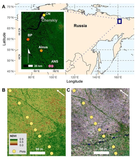
Figure 1.
A map of the study area in northeastern Siberia, Russia. Panel (A) shows the location of the study area in Northeastern Siberia, Russia outlined by the blue box, which highlights the area of the inset map. The inset map shows the location of the transects that are labeled with a background of a composite Landsat image. Panel (B) shows the NDVI image calculated from the multispectral UAV data for the CN transect 1. Panel (C) shows the visible spectrum (RGB) UAV data for the CN transect 1.
2.2. Field Data
Field data from the four burn perimeters that corresponded to UAV data was collected during the summers of 2018 and 2019. Field data were collected along seven 250-m transects within the burn perimeters (1–2 transects per burn), running from 50-m into the unburned area to 200-m into the burned area. Each transect consisted of eight plots. We collected GPS coordinates at the center of each plot. Trees were sampled within a 4–10 m radius plot from plot center, with plot size decreasing with increasing density of live and dead trees. Tall deciduous shrubs were sampled in a variable-width (0.5–1 m), 5-m length belt transect running from plot center to the north in the northwest quadrant of the plot. The width of the belt transect was reduced when shrub density was high. Field data were aggregated to plot-level aboveground carbon biomass and basal area of trees and shrubs. Tree [20] and shrub [43] biomass were calculated individually as grams per square meter (Table 1). Then biomass was converted to aboveground carbon biomass as grams of carbon per meter square using a carbon concentration of 46% for live trees [20] and 48% for tall shrubs [21]. Live trees and shrubs were combined to estimate aboveground woody carbon biomass. Live tree and shrub basal area were each calculated per plot and scaled up to meters squared per hectare. These variables were selected for analysis to determine how woody vegetation cover influences vegetation indices in these ecosystems.

Table 1.
Details for the allometric equations used to calculate biomass for field-based measures of trees [20] and shrubs [43]. The equation was biomass = ax^b (x = BD or DBH), where values for a and b are listed in the table and correspond to the basal diameter (BD) or diameter at breast height (DBH) of the field-based measures [20,43].
2.3. UAV Data Collection
We collected both RGB and multispectral imagery using a DJI Phantom 4 Advanced quadcopter (Table 2). The RGB imagery was obtained with the stock camera (1-inch [i.e., 13.2 × 8.8 mm] 20 MP CMOS sensor) on the Phantom 4 Advanced quadcopter. Multispectral imagery was collected with a Parrot Sequoia multispectral camera mounted to a Phantom 4 Advanced quadcopter using custom 3D printed mounts. Multispectral Sequoia imagery consists of four bands collected with the following separate monochrome sensors (~1 MP resolution)—green 530–570 nm, red 640–680 nm, red-edge 730–740 nm, and near-infrared 770–810 nm. The Sequoia has an integrated irradiance sensor that was mounted to the top of the quadcopter to account for any changes in illumination during the flight. In addition, pre- and post-flight images of a calibrated reflectance panel (60% broadband reflectance, Micasense, Seattle, WA, USA) were used to convert at sensor radiance to reflectance. Flight collection protocols were based on those developed by the High Latitude Drone Ecology Network (HiLDEN) [44]. Briefly, the imagery was collected as close as possible to local solar noon, and flights at each site were centered on the sampling transect. Sky condition was generally clear, though cloud cover was unavoidable and affected several flights. The additional payload associated with the Parrot Sequoia reduced battery life and affected aircraft maneuverability. Therefore, it was not possible to collect multispectral imagery on all transects. Thus, RGB imagery was available for all seven transects, while multispectral imagery was only available for four of the seven transects. Flights with only RGB were flown at 120 m altitude to maximize spatial coverage, while multispectral flights were flown at 60 m altitude to maximize spatial resolution (owing to the smaller ~1 MP sensor size). At each site, 5–10 0.25 m2 checkered nylon ground control targets were placed throughout the sample area, and the coordinates were recorded using two Emlid Reach RS+ RTK GPS receivers (St. Petersburg, Russia) with ~10 cm geometric accuracy. Images were orthorectified and mosaicked in Pix4D Mapper for multispectral (Pix4D S.A. Prilly, Switzerland) and Agisoft Metashape for RGB (Agisoft LLC, St. Petersburg, Russia), and co-registered using ground control points.
Table 2.
Collection details for visible spectrum (RGB) and multispectral (MS) data. All data were collected during the summer 2019. We report the field site code, field transect number, flight numbers for RGB/MS, year of burn, day of year (DoY) flight occurred, altitude of flight, and pixel resolution for processed imagery.
RGB and multispectral imagery was used to calculate vegetation indices. We calculated the GCC index for each pixel in the orthomosaic imagery for all seven transects. The GCC index is the ratio of green light radiance to total radiance for each pixel and calculated as
We used multispectral imagery to calculate the NDVI for each pixel as
The vegetation index values were extracted for each plot along the transect using a spatial buffer that extracted an aggregated mean based on the specified radius outlined below.
2.4. Data Analysis
We used correlation analysis and linear models to analyze our three research objectives that evaluate how GCC and NDVI: (1) relate to each other at varying spatial resolutions, (2) predict aboveground carbon biomass and basal area, and (3) distinguish burned, unburned, and edge effects. We used the cor and lm function from the ‘stats’ package for each analysis [45]. We assessed assumptions for all models by visually inspecting the residuals. All analyses were performed in the R Statistical Computing Software version 3.6.3 [45] with the ‘lsmeans’ [46] and ‘tidyverse’ packages [47]. Field data [48], UAV data [49], and code [50] for the analyses are available online.
To assess how GCC and NDVI relate to each other at increasing spatial resolutions (from 25 cm to 10 m), we performed a correlation analysis. For each spatial resolution, the vegetation index values were an aggregated mean of pixels extracted at an increasing radius of 25 cm, 50 cm, 1 m, 3 m, 5 m, and 10 m from the plot center. The buffer radius was measured from the GPS coordinates taken from the center of each field plot along the transect. We opted for this approach since the pixel resolutions were not consistent across all imagery (Table 2). Further, aggregating pixels over a spatial area into a mean pixel value improves linkages to coarser resolution satellite imagery [51], and spatial aggregations have been evaluated in several investigations e.g., [10,52,53,54]. The spatial scales were chosen to correspond to ecologically meaningful scales where finer resolutions are associated with an individual plant’s area, and coarser resolutions are associated with field plot sizes.
Second, we assessed how well GCC and NDVI predict field-based measures of aboveground carbon biomass and basal area of live trees and tall shrubs. We fit two models to predict aboveground carbon biomass, the first model with GCC and increasing spatial resolutions (25 cm, 50 cm, 1 m, 3 m, 5 m, and 10 m) as explanatory variables and a second model with NDVI and increasing spatial resolutions (25 cm, 50 cm, 1 m, 3 m, 5 m, and 10 m) as explanatory variables. The increasing spatial resolution was treated as a categorical variable. We log-transformed aboveground carbon biomass to meet model assumptions [55]. We assessed the relationship between the vegetation indices and basal area of live trees and shrubs, using the 10-m aggregated mean values for GCC and NDVI, based on the correlation analysis and assessment of standard deviations of aggregated means between GCC and NDVI. Four statistical models were run with each combination of response variables, live tree or tall shrub basal area, and explanatory variables, GCC or NDVI.
Lastly, we evaluated the difference in GCC and NDVI values between burned and unburned areas as well as how vegetation indices change across the field transect from the unburned into the burned area. We used the 10-m aggregated mean for GCC and NDVI based on the correlation analysis and evaluation of standard deviation spread. A Welch t-test [56] for unequal variance was performed to test for a difference in the means of GCC and NDVI between burned and unburned areas. We then regressed GCC and NDVI separately against distance from the unburned edge.
3. Results
3.1. Correspondence between GCC and NDVI
We were primarily interested in how GCC corresponded to NDVI at comparable spatial resolutions. The correlation between GCC and NDVI increased with increasing spatial resolution (e.g., aggregated mean based on increasing buffer radius; Table 3). GCC and NDVI were correlated most strongly with each other at the 3-m, 5-m, and 10-m resolutions (ρ > 0.91) compared to finer resolutions (1-m or less). Standard deviations of the aggregated means were evaluated to assess variability within each buffer resolution. The standard deviations increased with increasing spatial resolution and plateaued at 3-m, 5-m, and 10-m radii with comparable variability (Table 3, Figure 2).
Table 3.
Correlation coefficients between GCC and NDVI at increasing spatial resolution. All paired correlations are reported, but we are primarily interested in the correlation coefficients between GCC and NDVI for each radius. The correlations are assessing the relationship between GCC and NDVI for the mean pixel value of all pixels within a circular plot with the radius indicated. The radius was centered on the field plot locations.
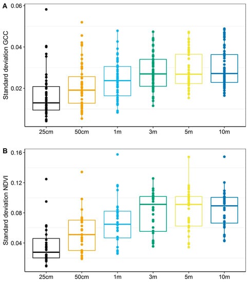
Figure 2.
Standard deviations for aggregated means to assess variability in GCC (A) and NDVI (B) within plots of increasing spatial resolution. For both GCC and NDVI, the standard deviation is smaller for finer spatial resolutions, and increases with increasing spatial resolution till 3-m radius at which point the standard deviations plateau. The plateau indicates that the 3-m, 5-m, and 10-m have comparable variability. The patterns illustrate that GCC and NDVI exhibit similar patterns of heterogeneity.
3.2. Linking Field-Based Measures and Vegetation Indices
We found that aboveground carbon biomass ranged between 116.7 and 6846.0 g C m−2 across the field plots. Aboveground carbon biomass increased with increasing GCC or NDVI (Figure 3; Table 4). NDVI was a better predictor of aboveground carbon biomass (R2 = 0.55) than GCC (R2 = 0.41). The 3-m, 5-m, 10-m resolution demonstrated stronger relationships between aboveground carbon biomass and GCC as well as NDVI.
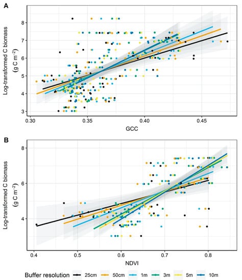
Figure 3.
Linear models testing how well log-transformed aboveground carbon biomass (C mass) is predicted by GCC (A) and NDVI (B) across increasing spatial resolutions. C mass includes trees and tall deciduous shrubs. Vegetation index values were an aggregated mean extracted at an increasing buffer radius (buffer resolution). Panels show fitted relationship with 95% confidence intervals and raw point data. NDVI (B) was a stronger predictor of C biomass than GCC (A) based on adjusted R2 (Table 4).
Table 4.
Linear models testing how well log-transformed aboveground carbon biomass (C mass) is predicted by GCC and NDVI across increasing spatial resolutions. Aboveground carbon biomass includes live trees and tall deciduous shrubs. Vegetation index values were an aggregated mean extracted at an increasing buffer radius. For each model, we report estimates of the coefficients (ß) for the y-intercept and slope, Standard Error (SE), the test statistic value (t), p-value, and adjusted R2. Statistical relationships are visualized in Figure 3.
The analyses showed that basal area of shrubs and trees increased with increasing GCC and NDVI (Figure 4; Table 5). Live tree basal area ranged from 0.00 to 34.57 m2 per hectare (ha). Shrub basal area ranged from 0.87 m2 per ha to 28.14 m2 per ha. GCC was a poor predictor of live tree (R2 = 0.14) and shrub basal area (R2 = 0.29). NDVI was a strong predictor of live tree basal area (R2 = 0.52), but a poor predictor of shrub basal area (R2 = 0.28).
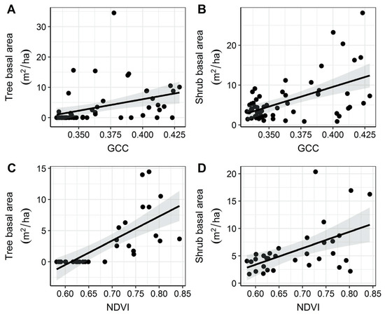
Figure 4.
Linear models testing for a relationship between vegetation indices and basal area (BA). Graphs show fitted relationship with 95% confidence intervals and raw point data. Shrub basal area was not predicted well by GCC (B; R2 = 0.29) or NDVI (D; R2 = 0.28). Tree basal area was predicted poorly by GCC (A; R2 = 0.14) and was predicted best by NDVI (C; R2 = 0.52).
Table 5.
Linear models testing how the aggregated means of GCC or NDVI with a 10-m buffer radius predict field-based measures of live tree and shrub basal area. For each model, we report the estimates of the coefficients (ß) for the y-intercept and slope, Standard Error (SE), the test statistic value (t), p-value, and adjusted R2. Statistical relationships are visualized in Figure 4.
3.3. Burned, Unburned, and Edge Effects
We found that the ranges in vegetation indices overlapped for burned and unburned forest. GCC ranged from 0.333 to 0.423 for burned and from 0.342 to 0.429 for unburned. NDVI ranged from 0.577 to 0.734 for burned and from 0.688 to 0.777 for unburned. GCC in burned (mean = 0.359) areas was statistically lower than in unburned areas (mean = 0.382), with a difference of −0.033 ± 0.009 (p = 0.016; Figure 5; Table 6). NDVI was also statistically lower in burned (mean = 0.639) versus unburned (mean = 0.728) areas, with a difference of −0.089 ± 0.017 (p-value < 0.0001; Figure 5; Table 6). From the unburned edge into the burn, vegetation index values declined with increasing distance from the unburned edge to 200-m into the burn (Figure 6; Table 7). GCC declined with increasing distance from the unburned edge with an estimate of ~0.379 at 50 m and of ~0.354 at 200 m into the burn perimeter (Figure 6; Table 7), which can be seen in the imagery (Figure 7). NDVI declined with increasing distance from the unburned edge with estimates of ~0.717 at 50 m and of ~0.592 at 200 m into the burn perimeter (Figure 6; Table 7), which can be seen in the imagery (Figure 7). The GCC and NDVI imagery of the four transects show the change over the transect from unburned into the burned (Figure 7).
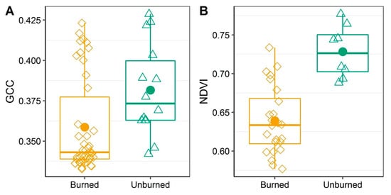
Figure 5.
A comparison between burned and unburned pixels for mean GCC (A) and NDVI (B) with a 10-m buffer radius. Boxplots indicate quartile distribution with raw data for burned (diamonds) and unburned (triangles) plots. The estimated mean is the point. A Welch t-test for unequal variance was performed to test for a difference in the means of GCC (A) and NDVI (B) between burned and unburned areas.
Table 6.
A Welch t-test for unequal variance was performed to test for a difference in the means of GCC and NDVI (using 10-m buffer radius) between burned and unburned areas. For each model, we report the response variable, estimated mean of burned (ß1), estimated mean of unburned (ß2), estimated difference in means (ß3), standard error for the difference in means (SE), the test statistic value (t), and p-value. Data are visualized in Figure 5.
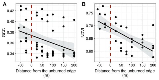
Figure 6.
Linear models assessing the relationship between aggregated mean GCC (A) and NDVI (B) with a 10-m buffer radius and distance from the unburned edge into the fire perimeter. The zero dashed line indicates the edge of the fire perimeter. To the right of zero is the burned area and to the left is the unburned area. Both vegetation indices show a decline in values moving from the unburned into the burned. Panels show fitted relationship with 95% confidence intervals and raw data points. Raw data points show the variability in vegetation index values across the transects.
Table 7.
Linear regression analyses of distance from unburned forest edge versus mean GCC or mean NDVI values using a 10-m buffer radius. Two statistical models were fit, one for GCC and one for NDVI. For each model, we report the response variable, estimates of the coefficients (ß) for the y-intercept and slope, standard error (SE), the test statistic value (t), p-value and adjusted R2. These models and raw data are visualized in Figure 6.
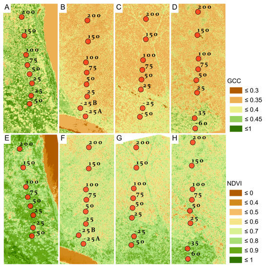
Figure 7.
GCC (A–D) and NDVI (E–H) imagery calculated from UAV imagery that corresponds to field transects. Alnus transect 1 burned in 1984 (A,E). BP transect 2 burned in 1983 (B,F). CN transect 1 burned in 2001 (C,G). CN transect 2 burned in 2001 (D,H). Plot locations are labeled with negative values indicating field plots on the unburned portion of the transects and positive values indicating distance into the burn in meters. Edges of fires were identified prior to the field campaign with satellite imagery.
4. Discussion
We found that both GCC and NDVI derived from UAV data serve as useful indicators of post-fire vegetation conditions in Cajander larch forests. Our results demonstrate the utility of UAV imagery for quantifying fine-scale variation in vegetation dynamics in landscapes where field access and availability of high-resolution satellite imagery are limited. GCC and NDVI were most strongly correlated at coarser spatial resolution (e.g., 3-m, 5-m, and 10-m radii) compared to finer spatial resolutions (e.g., 1-m or less), which is likely due to minimizing the effects of background reflectance. Aboveground carbon biomass was predicted best by NDVI at 3-m, 5-m, and 10-m radii, which makes sense given the scale of field sampling and the fact that fine resolutions capture the heterogeneity of an individual plant rather than patches dominated by different plant functional groups [10]. NDVI may perform better than GCC in predicting biomass because it is derived from radiometrically calibrated imagery, and includes near-infrared and red wavelengths that capture the spectral characteristics of plants. In contrast, the visible bands used to calculate GCC may be more sensitive to radiation reflected from non-photosynthetic surfaces. These findings highlight the importance of spatial resolution for linking UAV and field-based measures. NDVI was a stronger predictor of live tree basal area compared to GCC, and neither vegetation index was a strong predictor of shrub basal area. Both indices seem to distinguish between burned, unburned, and visualizations indicate a distinguishable edge effect. For GCC, the range of values across both burned and unburned matches observations in other vegetation studies [57,58]. For NDVI, the range of values across both burned and unburned is characteristic of landscapes dominated by shrubs or a mixture of shrubs and trees with an open canopy structure [12,59]. These findings illustrate the utility of UAV data for NDVI in this region as a tool for quantifying and monitoring the post-fire ecological response.
4.1. Correspondence between GCC and NDVI
The relationship between GCC and NDVI demonstrates the utility of GCC for characterizing spatial heterogeneity of vegetation in high-latitude Cajander larch forests. To date, there has been limited evaluation of spatial correspondence between GCC and NDVI. Vegetation indices derived from RGB and multispectral imagery are comparable for measuring phenology of plant green-up [60]. Commercial, off-the-shelf UAV units with integrated RGB cameras are cheaper and easier to use than stand-alone multispectral cameras that must often be integrated with a UAV by the user. However, radiometrically calibrating RGB imagery is less straightforward, meaning that images may vary with illumination condition, and this may have contributed to the variability in our results. While UAV with built-in multispectral cameras are becoming more readily accessible, they are considerably more expensive than consumer UAV, such as the DJI Phantom 4 that we used. The GCC index provides a robust measure of greenness for measuring spatial and temporal variation in temperate conifer forests [36,37], Mediterranean pine forests [35], and assessing forest stand vigor in North American sub-boreal systems [61]. Testing the viability of vegetation indices calculated from RGB is timely since UAVs are becoming more financially accessible and can accelerate data acquisition in post-fire landscapes [34,62]. Our results demonstrate that the ability to acquire high resolution imagery in remote landscapes provides useful new opportunities to improve overall understanding of vegetation dynamics and provide valuable context for freely available coarse resolution satellite imagery.
A larger radius for pixel aggregation resulted in a better correspondence between NDVI and GCC, indicating that a coarser spatial resolution improves the signal to noise ratio. The finest spatial resolution (25-cm radius) may merely be capturing the reflectance from one component of the broader landscape like a patch of lichen/moss or a single shrub, while the coarser resolution (10-m radius) is aggregating the reflectance of these distinct vegetation components into a single vegetation index value. These landscapes have substantial variation in biomass, plant communities and structure that contribute to spectral heterogeneity. Aggregating pixels is considered an appropriate measure for minimizing the influence of vegetation heterogeneity on spectral index values [10,63] and relevant for evaluating linkages between field-based measures and UAV data [10]. Aggregating pixels over a spatial area into a mean pixels value improves linkages to coarser resolution remote sensing imagery [51], and spatial aggregations have been evaluated in several investigations e.g., [10,52,53,54]. This finding indicates that the spatial resolution is important, and the patchiness of these ecosystems influences each vegetation index. Continued research is needed to determine why GCC and NDVI agree less well at smaller spatial scales, with field observations at similarly small scales to determine the ecological drivers of this mismatch [10].
4.2. Linking Field-Based Measures and Vegetation Indices
NDVI was a stronger predictor of aboveground carbon biomass compared to GCC. This finding points to the value of multispectral imagery from UAVs in this region. The 3-m, 5-m, and 10-m resolution demonstrated stronger relationships with field-based measures, pointing to the importance of scale [63] and multispectral imagery for these ecosystems. The composition and structure of larch forests can be variable and patchy across the landscape [20,21] and contributes to spectral heterogeneity [10,12,64]. This finding suggests that NDVI could serve as a proxy for aboveground carbon biomass, and indicates that commercial high-resolution satellite data (e.g., PlanetScope or Worldview) have sufficiently high spatial resolution to capture variation in biomass as well. However, previous evaluations on this landscape found no relationship between larch aboveground carbon biomass and NDVI sampled at high to moderate spatial resolution (3–30 m) using PlanetScope and Landsat imagery [12]. This, in conjunction with our results, highlights the potential importance of understory shrub biomass, and suggests that UAV-imagery may serve as an important linkage between field-based and satellite-based measures of ecosystem characteristics related to vegetation [10]. Targeted work aimed at understanding how relationships between vegetation indices and field measurements of vegetation vary with spatial scale and plant functional type is necessary to integrate linkages between UAV and satellite imagery.
NDVI predicted tree basal area better than GCC, while neither index predicted shrub basal area well. Forest landscapes consist of vertical and horizontal heterogeneity, and evaluating a single component of the vegetation structure may not necessarily be well represented by vegetation indices that are measuring all vegetation in an area. While tree or shrub basal area generally increased with increasing vegetation index values, this is expected given that photosynthetic biomass scales allometrically with the basal area for both trees and shrubs in these ecosystems [20,43,65]. However, tree and shrub abundance only explained a portion of the variation in vegetation indices, and graminoids and non-vascular plants also exert a strong influence on NDVI at fine scales in ecosystems in this region [59,66]. This suggests that more detailed vegetation community sampling across fire boundaries, coupled with UAV surveys, may help to elucidate post-fire understory vegetation dynamics in these ecosystems.
Individual pixels from either UAV or satellite imagery represent a mixture of spectral signatures due to the heterogeneous structure of shrubs and trees, that from a top-down view are composed of leaves and woody material associated with twigs, branches, and stems. Further heterogeneity is introduced by spectral differences between patches of non-vascular vegetation or bare ground visible through gaps in tree and shrub canopies. This mixture of materials means that, at all but the finest spatial resolution, a single pixel captures characteristics that are a combination of surface types [67], and represents a continued challenge for linking field data with remote sensing imagery [12]. While finer spatial resolution has the potential to mitigate this issue, it will require field sampling at finer scales as well. Still, the heterogeneity will be a consistent component of optical remote sensing in these ecosystems as vegetation patches can be as small as ~50 cm in diameter [59].
4.3. Postfire Vegetation Index Patterns Across Burn Perimeters
Both vegetation indices clearly differentiated burned and unburned areas in even the oldest fire scars, supporting the notion that larch forests are slow to recover and return to pre-fire greenness levels measured by reflectance [20,64]. These findings align with the general understanding that larch seedlings are slow-growing and often obscured by tall shrubs for one to two decades post-fire. The short growing season and slow growth of Cajander larch results in a protracted contribution of larch to total ecosystem biomass [4,64]. In comparison, tree biomass in North American boreal forests accumulates more rapidly [68,69], resulting in mappable forest recovery trajectories [70]. Satellite-based studies have shown the recovery in greenness measured by vegetation indices takes more than a decade across high latitude regions of the northern hemisphere [4,64,71]. However, this delayed recovery is measured with MODIS, a coarse spatial resolution (0.5–1 km) satellite, that minimizes variability in landscape heterogeneity captured by the finer spatial scale UAV data. In southern Siberian forests, post-fire recovery is linked with fire frequency, burn severity, and surface temperature anomalies, where more severe burns show greater spectral recovery rates [72].
Declines in GCC and NDVI with increasing distance from the burn perimeter illustrate edge effects that persist for several decades post-fire that are detectable with remote sensing imagery. However, post-fire reflectance signatures are most likely dominated by understory vegetation because seedling regeneration is slow, and seedlings are quite small. The edges of fire perimeters serve as seed sources for areas within the burn perimeter [73] and have been shown to influence plant assemblages in the North American boreal forests of Ontario [74,75]. Due to the monodominance of Cajander larch, these forests depend on trees that survive fire to serve as a seed source. It is feasible that greater seed rain would occur closer to the unburned forest edge in the absence of surviving trees within the burn perimeter. This proximity to seed source would create edge effects for larch that are potentially more prominent than those observed for other boreal forest trees where regeneration depends on serotinous seed sources or resprouting. However, because tree density in these forests is low, and larch recruitment typically occurs over several decades, it is likely that the edge effects we observed are related to understory vegetation recovery. An additional reason that NDVI and GCC might decrease with distance from the burned edge is that some of the burned edges were not discrete and there was a transitional zone with some live trees that survived the burn up to 25-50 m away from the primary burn edge.
Larch understory vegetation communities are similar to those found in tundra ecosystems, where recovery of vegetation productivity takes longer in areas with severe burning [76]. Consequently, it is feasible that the edge effects we observed were related to increasing soil organic layer combustion (i.e., burn severity) [77,78] with distance from the unburned edge whereby vegetation in less severely burned areas along the edge of the fire perimeter recovers faster. Declines in seed dispersal with distance from the unburned edge provide an alternative explanation, although many common understory non-vascular plants are known to resprout from surviving underground parts [76]. Continued research on spatial variation in burn severity, post-fire propagation, and edge effects are needed to elucidate drivers of reflectance gradients observed at the edge of fire perimeters in northeastern Siberia.
5. Conclusions
Our study illustrates useful relationships between field-based vegetation measures and UAV-derived vegetation indices across post-fire Cajander larch forests. We found that heterogeneity in vegetation indices varied with spatial resolution, and lead to differences in the ability of vegetation indices to explain variability in aboveground carbon biomass. The spectral distinctions between burned, unburned, and gradients across fire perimeters reveal edge effects associated with gradients of vegetation recovery that may be a consequence of post-fire ecological response, burn severity, understory vegetation dynamics, larch dispersal dynamics, or some combination of all these factors. Although NDVI generally corresponded more strongly with field observations, GCC also correlated with vegetation characteristics, highlighting the potential utility of easily accessible RGB sensors. Overall, our research demonstrates the utility of UAV data for documenting post-fire vegetation dynamics in Cajander larch forests, while also highlighting the need for continued research focused on understanding how relationships between vegetation and spectral indices vary across fine spatial scales.
Author Contributions
Conceptualization, E.F., H.K., M.M.L., A.C.T.; Data curation E.F., M.M.L., A.C.T, A.K.P.; Formal analysis, A.C.T.; Funding Acquisition, M.M.L. and H.D.A.; Investigation, E.F., M.M.L., A.K.P., H.D.A., J.D.; Resources, N.S.Z., S.Z.; Visualization, A.C.T.; Writing—original draft, A.C.T., M.M.L.; Writing—review and editing, H.K., A.K.P., H.D.A., J.D.; All authors have read and agreed to the published version of the manuscript.
Funding
This research was funded by the National Science Foundation, OPP-1708307 to H. Alexander and OPP-1708322 to M. Loranty.
Acknowledgments
We thank everyone in the field during 2019 including Eric Borth, Sarah Frankenberg, Seth Robinson, Amanda Ruland, and Jill Young. We thank the staff and scientists at the Northeast Science Station for logistical and field support. We thank Anders Knudby and Michelle Jones for helpful analytical conversations.
Conflicts of Interest
The authors declare no conflict of interest. The funders had no role in the design of the study; in the collection, analyses, or interpretation of data; in the writing of the manuscript, or in the decision to publish the results.
References
- Serreze, M.C.; Barry, R.G. Processes and impacts of Arctic amplification: A research synthesis. Glob. Planet. Chang. 2011, 77, 85–96. [Google Scholar] [CrossRef]
- Post, E.; Alley, R.B.; Christensen, T.R.; Macias-Fauria, M.; Forbes, B.C.; Gooseff, M.N.; Iler, A.; Kerby, J.T.; Laidre, K.L.; Mann, M.E.; et al. The polar regions in a 2 °C warmer world. Sci. Adv. 2019, 5, eaaw9883. [Google Scholar] [CrossRef] [PubMed]
- Chapin, F.S. Role of Land-Surface Changes in Arctic Summer Warming. Science 2005, 310, 657–660. [Google Scholar] [CrossRef] [PubMed]
- Beck, P.S.A.; Goetz, S.J. Satellite observations of high northern latitude vegetation productivity changes between 1982 and 2008: Ecological variability and regional differences. Environ. Res. Lett. 2011, 6. [Google Scholar] [CrossRef]
- Jia, G.J.; Epstein, H.E.; Walker, D.A. Greening of arctic Alaska, 1981–2001. Geophys. Res. Lett. 2003, 30, 2003GL018268. [Google Scholar] [CrossRef]
- Forbes, B.C.; Fauria, M.M.; Zetterberg, P. Russian Arctic warming and ‘greening’ are closely tracked by tundra shrub willows. Glob. Chang. Biol. 2010, 16, 1542–1554. [Google Scholar] [CrossRef]
- Frost, G.V.; Epstein, H.E. Tall shrub and tree expansion in Siberian tundra ecotones since the 1960s. Glob. Chang. Biol. 2014, 20, 1264–1277. [Google Scholar] [CrossRef]
- McManus, K.M.; Morton, D.C.; Masek, J.G.; Wang, D.; Sexton, J.O.; Nagol, J.R.; Ropars, P.; Boudreau, S. Satellite-based evidence for shrub and graminoid tundra expansion in northern Quebec from 1986 to 2010. Glob. Chang. Biol. 2012, 18, 2313–2323. [Google Scholar] [CrossRef]
- Assmann, J.J.; Myers-Smith, I.H.; Kerby, J.T.; Cunliffe, A.M.; Daskalova, G. Drone data reveal heterogeneity in tundra greenness and phenology not captured by satellites. Preprint 2020. [Google Scholar] [CrossRef]
- Siewert, M.B.; Olofsson, J. Scale-dependency of Arctic ecosystem properties revealed by UAV. Environ. Res. Lett. 2020. [Google Scholar] [CrossRef]
- Loranty, M.M.; Lieberman-Cribbin, W.; Berner, L.T.; Natali, S.M.; Goetz, S.J.; Alexander, H.D.; Kholodov, A.L. Spatial variation in vegetation productivity trends, fire disturbance, and soil carbon across arctic-boreal permafrost ecosystems. Environ. Res. Lett. 2016, 11, 095008. [Google Scholar] [CrossRef]
- Loranty, M.; Davydov, S.; Kropp, H.; Alexander, H.; Mack, M.; Natali, S.; Zimov, N. Vegetation Indices Do Not Capture Forest Cover Variation in Upland Siberian Larch Forests. Remote Sens. 2018, 10, 1686. [Google Scholar] [CrossRef]
- Berner, L.T.; Beck, P.S.A.; Bunn, A.G.; Goetz, S.J. Plant response to climate change along the forest-tundra ecotone in northeastern Siberia. Glob. Chang. Biol. 2013. [Google Scholar] [CrossRef] [PubMed]
- Stocks, B.J.; Fosberg, M.A.; Lynham, T.J.; Mearns, L.; Wotton, B.M.; Yang, Q.; Jin, J.-Z.; Lawrence, K.; Hartley, G.R.; Mason, J.A.; et al. Climate Change and Forest Fire Potential in Russian and Canadian Boreal Forests. Clim. Chang. 1998, 38, 1–13. [Google Scholar] [CrossRef]
- Groisman, P.Y.; Sherstyukov, B.G.; Razuvaev, V.N.; Knight, R.W.; Enloe, J.G.; Stroumentova, N.S.; Whitfield, P.H.; Førland, E.; Hannsen-Bauer, I.; Tuomenvirta, H.; et al. Potential forest fire danger over Northern Eurasia: Changes during the 20th century. Glob. Planet. Chang. 2007, 56, 371–386. [Google Scholar] [CrossRef]
- Soja, A.J.; Tchebakova, N.M.; French, N.H.F.; Flannigan, M.D.; Shugart, H.H.; Stocks, B.J.; Sukhinin, A.I.; Parfenova, E.I.; Chapin, F.S.; Stackhouse, P.W. Climate-induced boreal forest change: Predictions versus current observations. Glob. Planet. Chang. 2007, 56, 274–296. [Google Scholar] [CrossRef]
- Kasischke, E.S.; Verbyla, D.L.; Rupp, S.; McGuire, A.D.; Murphy, K.A.; Jandt, R.; Barnes, J.L.; Hoy, E.E.; Duffy, P.A.; Calef, M.; et al. Alaska’s changing fire regime—implications for the vulnerability of its boreal forests. Can. J. For. Res. 2010, 40, 1313–1324. [Google Scholar] [CrossRef]
- Ponomarev, E.; Kharuk, V.; Ranson, K. Wildfires Dynamics in Siberian Larch Forests. Forests 2016, 7, 125. [Google Scholar] [CrossRef]
- Johnstone, J.F.; Allen, C.D.; Franklin, J.F.; Frelich, L.E.; Harvey, B.J.; Higuera, P.E.; Mack, M.C.; Meentemeyer, R.K.; Metz, M.R.; Perry, G.L.; et al. Changing disturbance regimes, ecological memory, and forest resilience. Front. Ecol. Environ. 2016, 14, 369–378. [Google Scholar] [CrossRef]
- Alexander, H.D.; Mack, M.C.; Goetz, S.; Loranty, M.M.; Beck, P.S.A.; Earl, K.; Zimov, S.; Davydov, S.; Thompson, C.C. Carbon Accumulation Patterns During Post-Fire Succession in Cajander Larch (Larix cajanderi) Forests of Siberia. Ecosystems 2012, 15, 1065–1082. [Google Scholar] [CrossRef]
- Webb, E.E.; Heard, K.; Natali, S.M.; Bunn, A.G.; Alexander, H.D.; Berner, L.T.; Kholodov, A.; Loranty, M.M.; Schade, J.D.; Spektor, V.; et al. Variability in above- and belowground carbon stocks in a Siberian larch watershed. Biogeosciences 2017, 14, 4279–4294. [Google Scholar] [CrossRef]
- Myers-Smith, I.H.; Forbes, B.C.; Wilmking, M.; Hallinger, M.; Lantz, T.; Blok, D.; Tape, K.D.; Macias-Fauria, M.; Sass-Klaassen, U.; Lévesque, E.; et al. Shrub expansion in tundra ecosystems: Dynamics, impacts and research priorities. Environ. Res. Lett. 2011, 6, 045509. [Google Scholar] [CrossRef]
- Walker, L.R.; Wardle, D.A.; Bardgett, R.D.; Clarkson, B.D. The use of chronosequences in studies of ecological succession and soil development: Chronosequences, succession and soil development. J. Ecol. 2010, 98, 725–736. [Google Scholar] [CrossRef]
- Epstein, H.E.; Myers-Smith, I.; Walker, D.A. Recent dynamics of arctic and sub-arctic vegetation. Environ. Res. Lett. 2013, 8, 015040. [Google Scholar] [CrossRef]
- Alexander, H.D.; Natali, S.M.; Loranty, M.M.; Ludwig, S.M.; Spektor, V.V.; Davydov, S.; Zimov, N.; Trujillo, I.; Mack, M.C. Impacts of increased soil burn severity on larch forest regeneration on permafrost soils of far northeastern Siberia. For. Ecol. Manag. 2018, 417, 144–153. [Google Scholar] [CrossRef]
- Kharuk, V.I.; Ranson, K.J.; Dvinskaya, M.L.; Im, S.T. Wildfires in northern Siberian larch dominated communities. Environ. Res. Lett. 2011, 6, 045208. [Google Scholar] [CrossRef]
- Loranty, M.M.; Abbott, B.W.; Blok, D.; Douglas, T.A.; Epstein, H.E.; Forbes, B.C.; Jones, B.M.; Kholodov, A.L.; Kropp, H.; Malhotra, A.; et al. Reviews and syntheses: Changing ecosystem influences on soil thermal regimes in northern high-latitude permafrost regions. Biogeosciences 2018, 15, 5287–5313. [Google Scholar] [CrossRef]
- Riihimäki, H.; Luoto, M.; Heiskanen, J. Estimating fractional cover of tundra vegetation at multiple scales using unmanned aerial systems and optical satellite data. Remote Sens. Environ. 2019, 224, 119–132. [Google Scholar] [CrossRef]
- Dandois, J.P.; Olano, M.; Ellis, E.C. Optimal Altitude, Overlap, and Weather Conditions for Computer Vision UAV Estimates of Forest Structure. Remote Sens. 2015, 7, 13895–13920. [Google Scholar] [CrossRef]
- Wallace, L.; Lucieer, A.; Malenovský, Z.; Turner, D.; Vopěnka, P. Assessment of Forest Structure Using Two UAV Techniques: A Comparison of Airborne Laser Scanning and Structure from Motion (SfM) Point Clouds. Forests 2016, 7, 62. [Google Scholar] [CrossRef]
- Fraser, R.H.; Olthof, I.; Lantz, T.C.; Schmitt, C. UAV photogrammetry for mapping vegetation in the low-Arctic. Arct. Sci. 2016, 2, 79–102. [Google Scholar] [CrossRef]
- Juszak, I.; Iturrate-Garcia, M.; Gastellu-Etchegorry, J.-P.; Schaepman, M.E.; Maximov, T.C.; Schaepman-Strub, G. Drivers of shortwave radiation fluxes in Arctic tundra across scales. Remote Sens. Environ. 2017, 193, 86–102. [Google Scholar] [CrossRef]
- Palace, M.; Herrick, C.; DelGreco, J.; Finnell, D.; Garnello, A.; McCalley, C.; McArthur, K.; Sullivan, F.; Varner, R. Determining Subarctic Peatland Vegetation Using an Unmanned Aerial System (UAS). Remote Sens. 2018, 10, 1498. [Google Scholar] [CrossRef]
- Samiappan, S.; Hathcock, L.; Turnage, G.; McCraine, C.; Pitchford, J.; Moorhead, R. Remote Sensing of Wildfire Using a Small Unmanned Aerial System: Post-Fire Mapping, Vegetation Recovery and Damage Analysis in Grand Bay, Mississippi/Alabama, USA. Drones 2019, 3, 43. [Google Scholar] [CrossRef]
- Larrinaga, A.R.; Brotons, L. Greenness Indices from a Low-Cost UAV Imagery as Tools for Monitoring Post-Fire Forest Recovery. Drones 2019, 3, 6. [Google Scholar] [CrossRef]
- Sonnentag, O.; Hufkens, K.; Teshera-Sterne, C.; Young, A.M.; Friedl, M.; Braswell, B.H.; Milliman, T.; O’Keefe, J.; Richardson, A.D. Digital repeat photography for phenological research in forest ecosystems. Agric. For. Meteorol. 2012, 152, 159–177. [Google Scholar] [CrossRef]
- Keenan, T.F.; Darby, B.; Felts, E.; Sonnentag, O.; Friedl, M.A.; Hufkens, K.; O’Keefe, J.; Klosterman, S.; Munger, J.W.; Toomey, M.; et al. Tracking forest phenology and seasonal physiology using digital repeat photography: A critical assessment. Ecol. Appl. 2014, 24, 1478–1489. [Google Scholar] [CrossRef]
- Pearson, R.L.; Miller, L.D. Remote mapping of standing crop biomass for estimation of the productivity of the shortgrass prairie, Pawnee National Grasslands, Colorado. In Proceedings of the 8th International Symposium on Remote Sensing of the Environment, Ann Arbor, MI, USA, 2–6 October 1972; pp. 1357–1381. [Google Scholar]
- Rouse, J.W.; Haas, R.H.; Schell, J.A. Monitoring vegetation systems in the Great Plains with ERTS. In Proceedings of the 3rd ERTS Symposium, Washington, DC, USA, 10–14 December 1973; pp. 309–317. [Google Scholar]
- Alcaraz-Segura, D.; Chuvieco, E.; Epstein, H.E.; Kasischke, E.S.; Trishchenko, A. Debating the greening vs. browning of the North American boreal forest: Differences between satellite datasets. Glob. Chang. Biol. 2010, 16, 760–770. [Google Scholar] [CrossRef]
- Guay, K.C.; Beck, P.S.A.; Berner, L.T.; Goetz, S.J.; Baccini, A.; Buermann, W. Vegetation productivity patterns at high northern latitudes: A multi-sensor satellite data assessment. Glob. Chang. Biol. 2014, 20, 3147–3158. [Google Scholar] [CrossRef]
- Wulder, M.A.; Hilker, T.; White, J.C.; Coops, N.C.; Masek, J.G.; Pflugmacher, D.; Crevier, Y. Virtual constellations for global terrestrial monitoring. Remote Sens. Environ. 2015, 170, 62–76. [Google Scholar] [CrossRef]
- Berner, L.T.; Alexander, H.D.; Loranty, M.M.; Ganzlin, P.; Mack, M.C.; Davydov, S.P.; Goetz, S.J. Biomass allometry for alder, dwarf birch, and willow in boreal forest and tundra ecosystems of far northeastern Siberia and north-central Alaska. For. Ecol. Manag. 2015, 337, 110–118. [Google Scholar] [CrossRef]
- Assmann, J.J.; Kerby, J.T.; Cunliffe, A.M.; Myers-Smith, I.H. Vegetation monitoring using multispectral sensors—best practices and lessons learned from high latitudes. J. Unmanned Veh. Syst. 2018, 7, 54–75. [Google Scholar] [CrossRef]
- R Core Team. A language and environment for statistical computing. Computing 2020. [Google Scholar] [CrossRef]
- Lenth, R.V. Least-Squares Means: The R Package lsmeans. J. Stat. Softw. 2016. [Google Scholar] [CrossRef]
- Wickham, H.; Averick, M.; Bryan, J.; Chang, W.; McGowan, L.; François, R.; Grolemund, G.; Hayes, A.; Henry, L.; Hester, J.; et al. Welcome to the Tidyverse. J. Open Source Softw. 2019, 4, 1686. [Google Scholar] [CrossRef]
- Alexander, H.; Paulson, A.; DeMarco, J.; Hewitt, R.; Lichstein, J.; Loranty, M.; Mack, M.; McEwan, R.; Borth, E.; Frankenberg, S.; et al. Fire influences on forest recovery and associated climate feedbacks in Siberian Larch Forests, Russia, 2018–2019. Arct. Data Cent. 2020. [Google Scholar] [CrossRef]
- Loranty, M.; Forbath, E.; Talucci, A.; Alexander, H.; DeMarco, J.; Hewitt, R.; Lichstein, J.; Mack, M.; Paulson, A.; McEwan, R. Uncrewed aerial vehicle remote sensing imagery of postfire vegetation in Siberian larch forests 2018–2019. Arct. Data Cent. 2020. [Google Scholar] [CrossRef]
- Talucci, A.C. Code: FLARE UAV and vegetation analyses. Zenodo 2020. [Google Scholar] [CrossRef]
- Blan, L.; Butler, R. Comparing Effects of Aggregation Methods on Statistical and Spatial Properties of Simulated Spatial Data. Remote Sens. 1999, 65, 73–84. [Google Scholar]
- Chen, J.M. Spatial Scaling of a Remotely Sensed Surface Parameter by Contexture. Remote Sens. Environ. 1999, 69, 30–42. [Google Scholar] [CrossRef]
- Chen, J.M.; Chen, X.; Ju, W. Effects of vegetation heterogeneity and surface topography on spatial scaling of net primary productivity. Biogeosci. Discuss. 2013, 10, 4225–4270. [Google Scholar] [CrossRef]
- Jin, Z.; Tian, Q.; Chen, J.M.; Chen, M. Spatial scaling between leaf area index maps of different resolutions. J. Environ. Manag. 2007, 85, 628–637. [Google Scholar] [CrossRef] [PubMed]
- Räsänen, A.; Juutinen, S.; Aurela, M.; Virtanen, T. Predicting aboveground biomass in Arctic landscapes using very high spatial resolution satellite imagery and field sampling. Int. J. Remote Sens. 2019, 40, 1175–1199. [Google Scholar] [CrossRef]
- Welch, B.L. The Generalization of ’Student’s’ Problem when Several Different Population Variances are Involved. Biometrika 1947, 34, 28. [Google Scholar] [CrossRef] [PubMed]
- Moore, C.E.; Brown, T.; Keenan, T.F.; Duursma, R.A.; van Dijk, A.I.J.M.; Beringer, J.; Culvenor, D.; Evans, B.; Huete, A.; Hutley, L.B.; et al. Australian vegetation phenology: New insights from satellite remote sensing and digital repeat photography. Biogeosci. Discuss. 2016. [Google Scholar] [CrossRef]
- Berra, E.F.; Gaulton, R.; Barr, S. Assessing spring phenology of a temperate woodland: A multiscale comparison of ground, unmanned aerial vehicle and Landsat satellite observations. Remote Sens. Environ. 2019, 223, 229–242. [Google Scholar] [CrossRef]
- Loranty, M.M.; Berner, L.T.; Taber, E.D.; Kropp, H.; Natali, S.M.; Alexander, H.D.; Davydov, S.P.; Zimov, N.S. Understory vegetation mediates permafrost active layer dynamics and carbon dioxide fluxes in open-canopy larch forests of northeastern Siberia. PLoS ONE 2018, 13, e0194014. [Google Scholar] [CrossRef]
- Richardson, A.D.; Jenkins, J.P.; Braswell, B.H.; Hollinger, D.Y.; Ollinger, S.V.; Smith, M.-L. Use of digital webcam images to track spring green-up in a deciduous broadleaf forest. Oecologia 2007, 152, 323–334. [Google Scholar] [CrossRef]
- Reid, A.M.; Chapman, W.K.; Prescott, C.E.; Nijland, W. Using excess greenness and green chromatic coordinate colour indices from aerial images to assess lodgepole pine vigour, mortality and disease occurrence. For. Ecol. Manag. 2016, 374, 146–153. [Google Scholar] [CrossRef]
- Xue, J.; Su, B. Significant Remote Sensing Vegetation Indices: A Review of Developments and Applications. J. Sens. 2017, 2017, 1353691. [Google Scholar] [CrossRef]
- Woodcock, C.E.; Strahler, A.H. The factor of scale in remote sensing. Remote Sens. Environ. 1987, 21, 311–332. [Google Scholar] [CrossRef]
- Berner, L.T.; Beck, P.S.A.; Loranty, M.M.; Alexander, H.D.; Mack, M.C.; Goetz, S.J. Cajander larch (Larix cajanderi) biomass distribution, fire regime and post-fire recovery in northeastern Siberia. Biogeosciences 2012, 9, 3943–3959. [Google Scholar] [CrossRef]
- Kropp, H.; Loranty, M.M.; Natali, S.M.; Kholodov, A.L.; Alexander, H.D.; Zimov, N.S.; Mack, M.C.; Spawn, S.A. Tree density influences ecohydrological drivers of plant–water relations in a larch boreal forest in Siberia. Ecohydrology 2019, 12. [Google Scholar] [CrossRef]
- Curasi, S.R.; Loranty, M.M.; Natali, S.M. Water track distribution and effects on carbon dioxide flux in an eastern Siberian upland tundra landscape. Environ. Res. Lett. 2016, 11, 045002. [Google Scholar] [CrossRef]
- Ormsby, J.P.; Choudhury, B.J.; Owe, M. Vegetation spatial variability and its effect on vegetation indices. Int. J. Remote Sens. 1987, 1301–1306. [Google Scholar] [CrossRef]
- Johnstone, J.F.; Chapin, F.S.; Foote, J.; Kemmett, S.; Price, K.; Viereck, L. Decadal observations of tree regeneration following fire in boreal forests. Can. J. For. Res. 2004, 34, 8. [Google Scholar] [CrossRef]
- Johnstone, J.F.; Chapin, F.S. Effects of Soil Burn Severity on Post-Fire Tree Recruitment in Boreal Forest. Ecosystems 2006, 9, 14–31. [Google Scholar] [CrossRef]
- Frazier, R.J.; Coops, N.C.; Wulder, M.A. Boreal Shield forest disturbance and recovery trends using Landsat time series. Remote Sens. Environ. 2015, 170, 317–327. [Google Scholar] [CrossRef]
- Cuevas-González, M.; Gerard, F.; Balzter, H.; Riaño, D. Analysing forest recovery after wildfire disturbance in boreal Siberia using remotely sensed vegetation indices. Glob. Chang. Biol. 2009, 15, 561–577. [Google Scholar] [CrossRef]
- Shvetsov, E.G.; Kukavskaya, E.A.; Buryak, L.V.; Barrett, K. Assessment of post-fire vegetation recovery in Southern Siberia using remote sensing observations. Environ. Res. Lett. 2019, 14, 055001. [Google Scholar] [CrossRef]
- Johnstone, J.; Boby, L.; Tissier, E.; Mack, M.; Verbyla, D.; Walker, X. Postfire seed rain of black spruce, a semiserotinous conifer, in forests of interior Alaska. Can. J. For. Res. 2009, 39, 1575–1588. [Google Scholar] [CrossRef]
- Braithwaite, N.T.; Mallik, A.U. Edge effects of wildfire and riparian buffers along boreal forest streams: Edge effects of wildfire and riparian buffers. J. Appl. Ecol. 2012, 49, 192–201. [Google Scholar] [CrossRef]
- Harper, K.A.; Drapeau, P.; Lesieur, D.; Bergeron, Y. Forest structure and composition at fire edges of different ages: Evidence of persistent structural features on the landscape. For. Ecol. Manag. 2014, 314, 131–140. [Google Scholar] [CrossRef]
- Bret-Harte, M.S.; Mack, M.C.; Shaver, G.R.; Huebner, D.C.; Johnston, M.; Mojica, C.A.; Pizano, C.; Reiskind, J.A. The response of Arctic vegetation and soils following an unusually severe tundra fire. Philos. Trans. R. Soc. B Biol. Sci. 2013, 368, 20120490. [Google Scholar] [CrossRef] [PubMed]
- Narayanaraj, G.; Wimberly, M.C. Influences of forest roads and their edge effects on the spatial pattern of burn severity. Int. J. Appl. Earth Obs. Geoinf. 2013, 23, 62–70. [Google Scholar] [CrossRef]
- Burton, P.J.; Parisien, M.-A.; Hicke, J.A.; Hall, R.J.; Freeburn, J.T. Large fires as agents of ecological diversity in the North American boreal forest. Int. J. Wildland Fire 2008, 17, 754. [Google Scholar] [CrossRef]
© 2020 by the authors. Licensee MDPI, Basel, Switzerland. This article is an open access article distributed under the terms and conditions of the Creative Commons Attribution (CC BY) license (http://creativecommons.org/licenses/by/4.0/).