Article

Shear-Wave Tomography Using Ocean Ambient Noise with Interference

1
College of Meteorology and Oceanography, National University of Defense Technology, Changsha 410073, China
2
Department of Electronic Systems, Norwegian University of Science and Technology, 7491 Trondheim, Norway
3
Equinor ASA, Arkitekt Ebbells Vei 10, 7005 Trondheim, Norway
*
Author to whom correspondence should be addressed.
Remote Sens. 2020, 12(18), 2969; https://doi.org/10.3390/rs12182969
Submission received: 18 June 2020 / Revised: 13 August 2020 / Accepted: 21 August 2020 / Published: 11 September 2020
(This article belongs to the Special Issue Remote Sensing in Applied Geophysics)

Abstract

:
Ambient noise carries abundant subsurface structure information and attracts ever-increasing attention in the past decades. However, there are lots of interference factors in the ambient noise in the real world, making the noise difficult to be utilized in seismic interferometry. The paper performs shear-wave tomography on a very short recording of ocean ambient noise with interference. An adapted eigenvalue-based filter is adopted as a pre-processing method to deal with the strong, directional interference problem. Beamforming and the noise crosscorrelation analyses show that the filter works well on the noise recorded by the array. Directional energy is significantly suppressed and the background diffuse component of the noise is relatively enhanced. The shear-wave tomography shows a 4-layer subsurface structure of the area covered by the array, with relatively homogeneous distribution of the shear-wave velocity values in the top three layers and a complicated structure in the bottom layer. Moreover, 3 high-velocity zones can be recognized in the bottom layer. The result is compared with several other tomography results using different methods and data. It demonstrates that, although the ambient noise used in this paper is very short and severely contaminated, a reasonable tomography result can be obtained by applying the adapted eigenvalue-based filter. Since it is the first application of the adapted eigenvalue-based filter in seismic tomography using ambient noise, the paper proves the effectiveness of this technique and shows the potential of the technique in ambient noise processing and passive seismic interferometry.

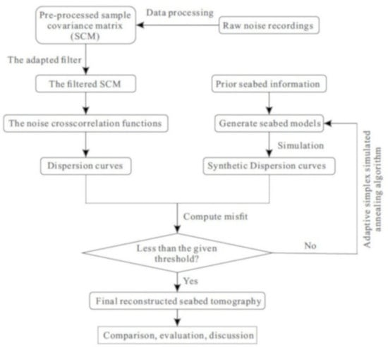
Graphical Abstract

1. Introduction

Passive seismic interferometry (PSI) makes use of the noise crosscorrelations (NCC) recorded by receiver pairs to reconstruct the subsurface impulse response. It turns one of the receivers in the pairs into a virtual source whose hypothetical reflection/energy is imaged by the other receiver. In this way, an estimate of the Green’s function between the receivers can be obtained [1,2]. The waves in the Green’s function usually carry much useful information of the environment between the receivers. This technique provides geophysicists a new perspective to view noise and study the structure of subsurface with no need for an active seismic source [3]. As an environmental-friendly passive imaging technique, PSI significantly enhances the importance of naturally occurring ambient noise and makes it possible to image subsurface structure and monitor temporal subsurface changes conveniently, environmental-friendly, and economically [4,5,6].
Aki [7] and Claerbout [8] developed the early framework of the technique. The theoretical basis of the technique was completed in the early 2000s [2,9,10,11,12,13]. Later, the application of the theory spreads in multiple research fields including seismology [1,8], helioseismology [14], ultrasonics [9], and underwater acoustics [15]. Nowadays, PSI has become a popular technique in subsurface tomography. Various applications have been done at different scales and for various purposes all over the world [16,17,18,19,20].
One of the key tasks of PSI is the reliable approximation of Green’s functions between receiver pairs. It requires that the noise field should be diffuse and equipartitioned [21,22]. Unfortunately, the noise field is usually contaminated by strong, directional sources in the real world, introducing biases into the approximated Green’s functions [23,24,25,26,27]. Wu et al. [22] reviewed the techniques which have been proposed to attenuate the interference of strong directional sources, and developed an adapted eigenvalue-based filter to improve the quality of the estimation of the Green’s function. The filter is adaptable for different data sets and can reduce the influence of strong, directional sources significantly.
The main objective of the paper is to perform shear-wave tomography on a very short recording of ocean ambient noise with interference and compare the tomographic picture obtained with other tomography results using active sources or much longer ambient noise recordings at the same field. The noise was recorded by a permanent reservoir monitoring receiver array (PRMRA) installed on the seabed of an offshore oil field in Norwegian North Sea. The adapted eigenvalue-based filter is applied as a pre-processing method to suppress the strong, directional interference in the recording and retrieve reliable approximations of Green’s functions. Note that the paper focuses on the same dataset with Wu et al. [22] but Wu et al. [22] focuses on the analysis of noise recording at one sensor, while this paper focuses on the whole data array.
The paper is organized as follows: First, we describe the array geometry and perform time and frequency analysis of the measured ambient noise. Then, we summarize the most important ideas of the adapted eigenvalue-based filter and apply the adapted eigenvalue-based filter to the measured ambient noise. Conventional beamforming is applied to the filtered sample covariance matrix (SCM) to evaluate the effectiveness of the adapted eigenvalue-based filter. The NCC is also retrieved based on the filtered SCM at this time. Later, the phase-speed dispersion curves are extracted and a 3D shear-wave tomography is performed. The result is compared with several previously published tomography results using different methods. Finally, we summarize the work and draw some conclusions.

2. Array Geometry and Noise Analysis

2.1. Array Geometry

The passive noise data were acquired by the PRMRA installed by Equinor in the Norwegian North Sea. The PRMRA contains 17 cables with length from 1.5 to 12.85 km, covering an area of approximately 50 km2. The Array Geometry is shown in Figure 1. The PRMRA is oriented in a 26–206° direction. The cable spacing is 300 m and the receiver spacing in cable is 50 m.

2.2. Noise Analysis

The noise data used here were continuously recorded by hydrophones in each receiver station for 1.02 h at a sampling rate of 500 Hz on 14 September 2015.

2.2.1. The ‘Natural Ambient Noise’

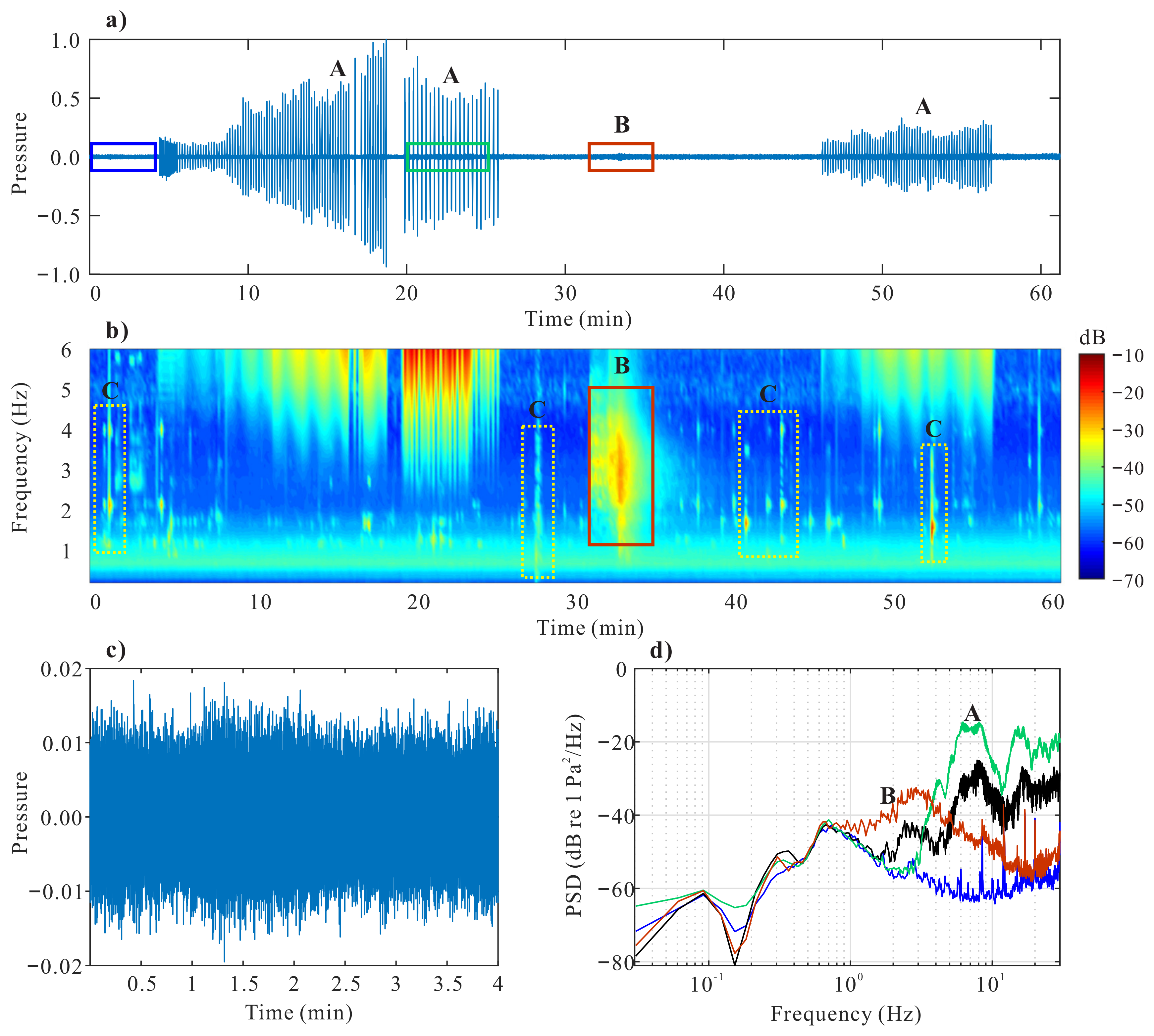
Figure 2a shows the noise recording on one receiver. Relatively speaking, the noise recordings marked with blue box in Figure 2a are not affected by severe events and can be denoted it as ‘natural ambient noise’. Figure 2c shows the enlarged view of the ‘natural ambient noise’ and Figure 2d presents the corresponding power spectral density (PSD) of it in blue. The PSD of the ‘natural ambient noise’ (blue) shows a peak at 0.7 Hz, which can be recognized as the peak of the microseisms in the ocean [28]. As the frequency increases from 0.7 Hz to 4.5 Hz, the PSD decreases gradually and no other peak appears. Actually, the frequency band of 0.2 to 4.5 Hz of the ocean ambient noise is usually dominated by the microseisms, which are believed to be generated by wind-related wave–wave interaction [28]. The microseisms are thought to be more evenly distributed in the ocean and the frequency band of 0.2 to 4.5 Hz is chosen to apply PSI in this paper.

2.2.2. Event A

In Figure 2a, waves with large amplitude (denoted as Event A) dominate the noise in the range of 4 to 26 min and 46 to 57 min. Figure 2b shows the averaged spectrogram of all receivers. Most of the energy of Event A spreads within the frequency band larger than 5 Hz. Part of the energy also affects the frequency band of 2 to 5 Hz considerably (especially in the time band of 20 to 26 min). Figure 2d presents the corresponding PSD of part of Event A (marked by a green box in Figure 2a) in green. It shows a similar peak with ‘natural ambient noise’ (blue) at 0.7 Hz but also shows increased energy beyond 2.5 Hz. 2 other higher peaks appears at about 8 Hz and 15 Hz.

2.2.3. Event B

In Figure 2a, Event B (marked by red box) happened during the period of 31 to 36 min. It is not obvious in the raw data. However, it becomes apparent in the spectrogram (solid red box in Figure 2b) and shows high energy in the frequency band of 1.5 to 5 Hz. Figure 2d presents PSD of Event B in red. It shows a similar trend to ‘natural ambient noise’ (blue) and Event A (green) below 0.7 Hz, but shows increased energy in the frequency band of 0.7 to 20 Hz. A higher peak appears at about 3 Hz.

2.2.4. Events C

Some other events can be recognized in the spectrogram (denoted as Events C and marked by dashed box in Figure 2b). These events have higher energy than the background noise and are usually generated by strong, directional sources.

2.2.5. Discussion of the Events

Overall, Figure 2d indicates that the PSD are clearly contaminated by Events A and B which are generated by strong and directional sources. The black curve shows the PSD of 60-min recordings. It describes the average effect of all events. Compared with the blue line, it shows increased energy beyond 1.5 Hz and is especially influenced by Events A and B.
The existence of Events A, B, and C are common and unpredictable in the real world. It damages the diffuse and equipartition property of the noise and bring challenges to the PSI.

2.2.6. Additional Insights on the Events

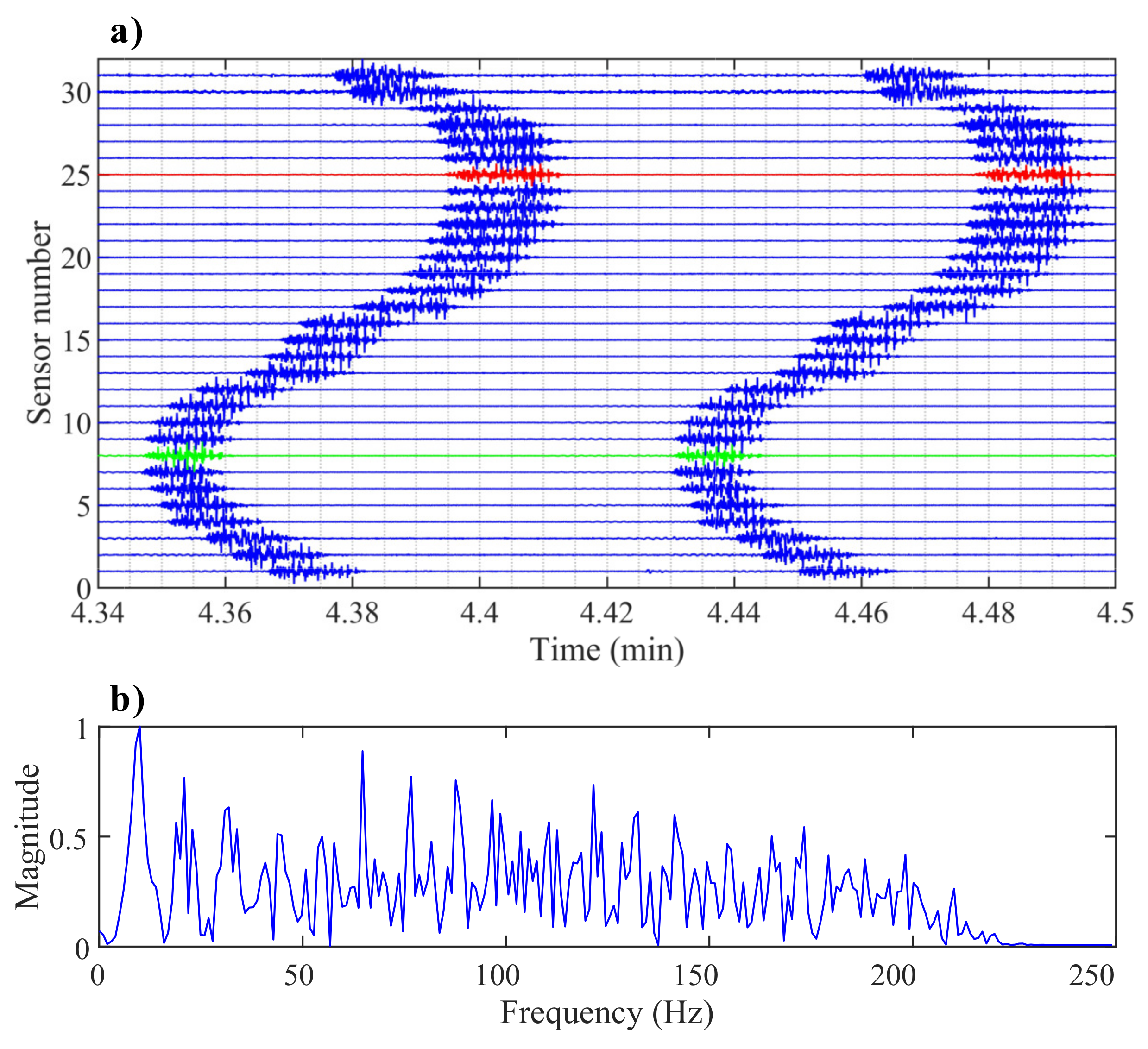
Figure 2 shows that Event A has a very regular time interval. The temporal and spectral signatures of Event A indicate that it comes from artificial sources which are very like airgun shots from other seismic surveys near this field. Unfortunately, there is no exact information available on these shots. In order to further study these signals, a travel time study is employed. Thirty-one sensors on the circle in Figure 1 are selected and numbered counterclockwise (with the red five-pointed star numbered as 1). Figure 3a shows the arrival time of the airgun signal on different sensors. The 4th sensor gets roughly the earliest arrival (green) and the 25th sensor gets the latest arrival (red). The 4th sensor and the 25th sensor are marked by a green asterisk and the red small circle in Figure 1, respectively. It indicates that the angle of incidence of the airgun shots is approximately 45° (the normal direction, which is perpendicular to the cable, is taken as a reference in the paper). The velocity of the signal is about 1450 m/s, which is estimated by travel time analysis. Figure 3b shows the spectrum of the signals in Figure 3a. It shows that the main energy of the airgun is concentrated in the frequency band of 3 to 200 Hz.
Figure 2b shows that the energy of Event B concentrate in the frequency band of 1.5 to 5 Hz. It fits the spectrum of earthquake very well [29]. Thus, it is possibly a small earthquake which lasts few minutes.

3. NCC Retrieval Using the Adapted Eigenvalue-Based Filter

Events similar to A, B, and C are unavoidable and unpredictable in the real world, challenging the accuracy and stability of the PSI. The adapted eigenvalue-based filter can help to mitigate the influence of these events and obtain improved NCC [22]. We apply the adapted eigenvalue-based filter to the noise data recorded by the PRMRA. In the following subsections, we summarize the basic ideas of the adapted eigenvalue-based filter (a detailed description can be found in [22]) and retrieve the NCC from the contaminated noise data using the adapted eigenvalue-based filter.

3.1. An Overview of the Adapted Eigenvalue-Based Filter

The main operation of the adapted eigenvalue-based filter is carried out on the SCM R ^ f . Supposing that the noise records are segmented into M segments, the SCM R ^ f can be computed by
R ^ f = 1 M m = 1 M u m f u m f H ,
where u m f is the Fourier coefficients vector of the noise records at a particular frequency f and H denotes Hermitian transpose.
The adapted eigenvalue-based filter tries to separate the SCM into different components as
R ^ = k = 1 K λ ^ k v ^ k v ^ k H + k = K + 1 N λ ^ k v ^ k v ^ k H + k = N + 1 N λ ^ k v ^ k v ^ k H = R ^ s + R ^ d + R ^ i ,
where λ ^ k (ascending order) and v ^ k are the eigenvalues and eigenvectors of R ^ , respectively, R ^ s is the strong, directional noise-related component, R ^ d is the diffuse noise-related component, and R ^ i is the uncorrelated noise-related component. The objective of the separation is to get a wavefield which is closer to be equipartitioned by suppressing R ^ s and R ^ i in the SCM.
The key point of the separation is the determination of values for N and K. N is called the cutoff number. Eigenvalues smaller than λ ^ N are thought to be related to uncorrelated noise (such as electronic noise and sensor self-noise) and are filtered. N can be determined by a theoretically derivation based on the geometry and degrees of freedom of the wavefield [22,30]. Eigenvalues larger than λ ^ K are thought to be related to strong, directional sources and need to be suppressed. A statistical hypothesis test is applied to determine the value of K [22]. By comparing the largest eigenvalues of the SCM and the statistical model of the ideal SCM (generated by diffuse, equipartitioned wavefield), all the eigenvalues larger than λ ^ K will be rejected. The weight of the hypothesis test enhances the effectiveness of the adapted eigenvalue-based filter and makes it more adaptable for different datasets.
The basic strategies to determine K and N are provided in Appendix A. Once the values for K and N are determined, we can obtain the filtered SCM R ^ i j f by suppressing R ^ s and R ^ i . The time-domain NCC function C i j f is defined as
C i j f = 0 T s i τ s j τ + t d τ ,
where s i f and s j f denote the ambient-noise records obtained by receivers i and j, respectively, and T denotes the observation period. In the frequency domain, given the filtered SCM R ^ f , we can compute the NCC of the data as
C ^ i j f = F 1 [ R ^ i j f ] ,
where F 1 denotes the inverse Fourier transform, f denotes the frequency, and R ^ i j f denotes the entry of R ^ f .

3.2. The Result

3.2.1. Beamforming

Wu et al. [22] studied one straight cable of the PRMRA and showed the good effect of the adapted eigenvalue-based filter. Since the PRMRA covers an area of 50 km2, local environments for different sensors and the coherence of the noise sources around different sensors may be different. It is necessary to study the application of the adapted eigenvalue-based filter to the entire array further. The study is also valuable for the shear-wave tomography in the following section.
To investigate the directionality of the wavefield, conventional beamforming is applied to the data recorded by different gathers (choose 30 continuously adjacent sensors in one cable as a gather, as is marked in red in Figure 1, for example). If the wavefield is diffuse and equipartitioned, the beamforming energy should be evenly distributed in all directions. An empirical estimation of the average phase speed 900 m/s is used in the beamforming. Although the estimation is rough, it does not make a big difference and is good enough to show the distribution of incoming energy. In addition, an iterative study can be done after the dispersion curves of the surface wave are extracted if it is necessary.
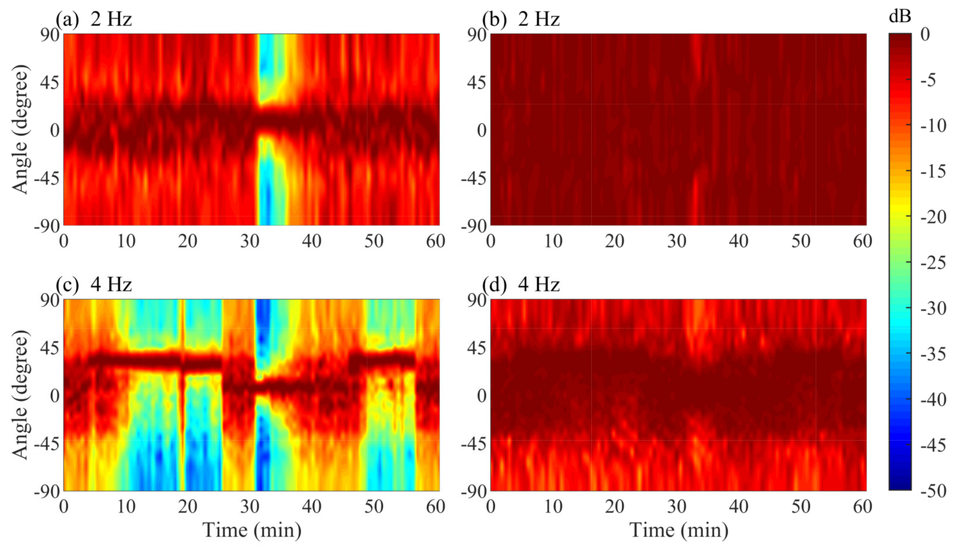
Figure 4 shows the beamforming result of one gather which is marked in red in Figure 1. Figure 4a,c show the beamforming energy distribution of the original wavefield. The energy is higher in the directions of −20° to 20° in Figure 4a than the background level. The energy becomes extraordinarily high from 30 to 40 min at 0° and can be recognized as Event B considering the high consistency in time and frequency. It indicates that Event B comes from the normal direction of the array. In Figure 4c, a source dominates the beam power with an almost constant direction of about 40°. It can be recognized as Event A considering the high consistency in time. The travel time study of Event A shows the incident angle of the airgun shots is approximately 45°. The misfit is caused by the usage of averaged phase speed in the beamforming. Figure 4a,c indicate that the original wavefield is affected by several strong, directional sources at both 2 Hz and 4 Hz. Event C, however, is not visible in the beamforming results because they have relatively lower energy than other events.
Figure 4b,d illustrate the beamforming energy distribution of the filtered wavefield using the adapted eigenvalue-based filter. Figure 4b,d show relatively uniform distributed energy compared with Figure 4a,c. It indicates that the adapted eigenvalue-based filter can suppress most of the high energy and partially recover the expected diffuse and equipartitioned wavefield.
Keeping all the parameters (especially the weight) of the adapted eigenvalue-based filter the same, similar results have been obtained for other gathers. It indicates that the influence of non-microseismic events on the receiver array over 50 km2 is more or less the same and that the adapted eigenvalue-based filter and the parameters used keep effective at the scale of 50 km2.

3.2.2. The NCC Retrieval

Selecting 30 continuously adjacent sensors in one cable as a gather and 25 sensors as the overlap between the adjacent gathers, 573 gathers are obtained from the entire PRMRA. We have retrieved the NCC for all gathers using Equation (4).
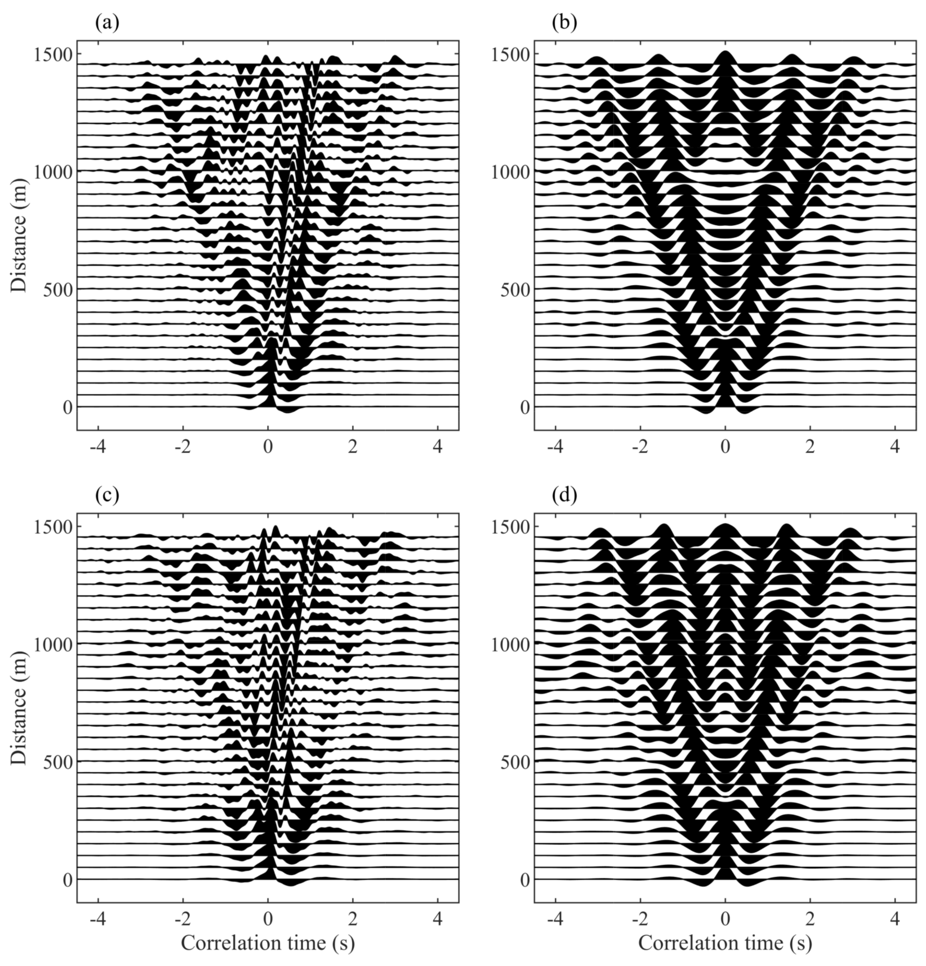
Figure 5 displays the NCC results for two gathers marked in red (Figure 5a,b) and green (Figure 5c,d) in Figure 1. All the NCCs are bandpass filtered between 0.2 and 4.5 Hz. Figure 5a,c displays the NCC retrieved from unfiltered SCM. The waveforms are apparently contaminated by directional, energetic events. The NCCs in Figure 5a uses the same gather with beamforming in Figure 4. The narrow peaks (close to 0 s) traveling with a velocity of about 1450 m/s are nondispersive and can be recognized as Event A. However, the effect of Events B and C is not very tyical in the NCC, making it hard to recognize. The existence of these directional, energetic events shields the expected surface waves severely. Figure 5b,d displays the NCC retrieved from the filtered SCM. Most of the influence of the directional, energetic events has been removed from the NCC and the expected surface waves are significantly enhanced. Figure 5b,d also show a clear dispersion feature, which is a typical characteristic for surface waves.
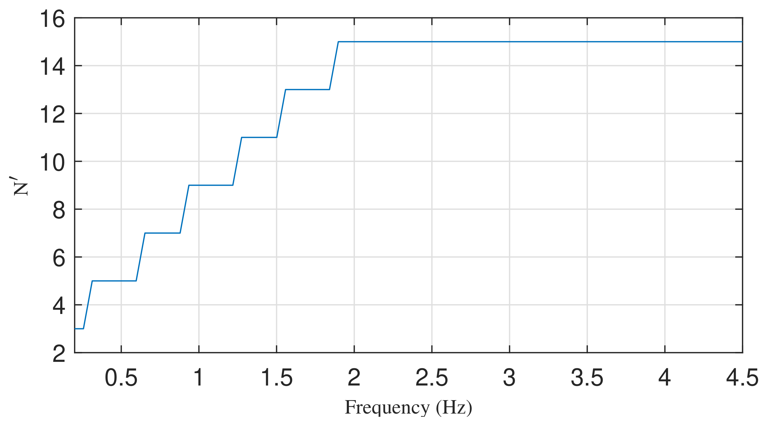
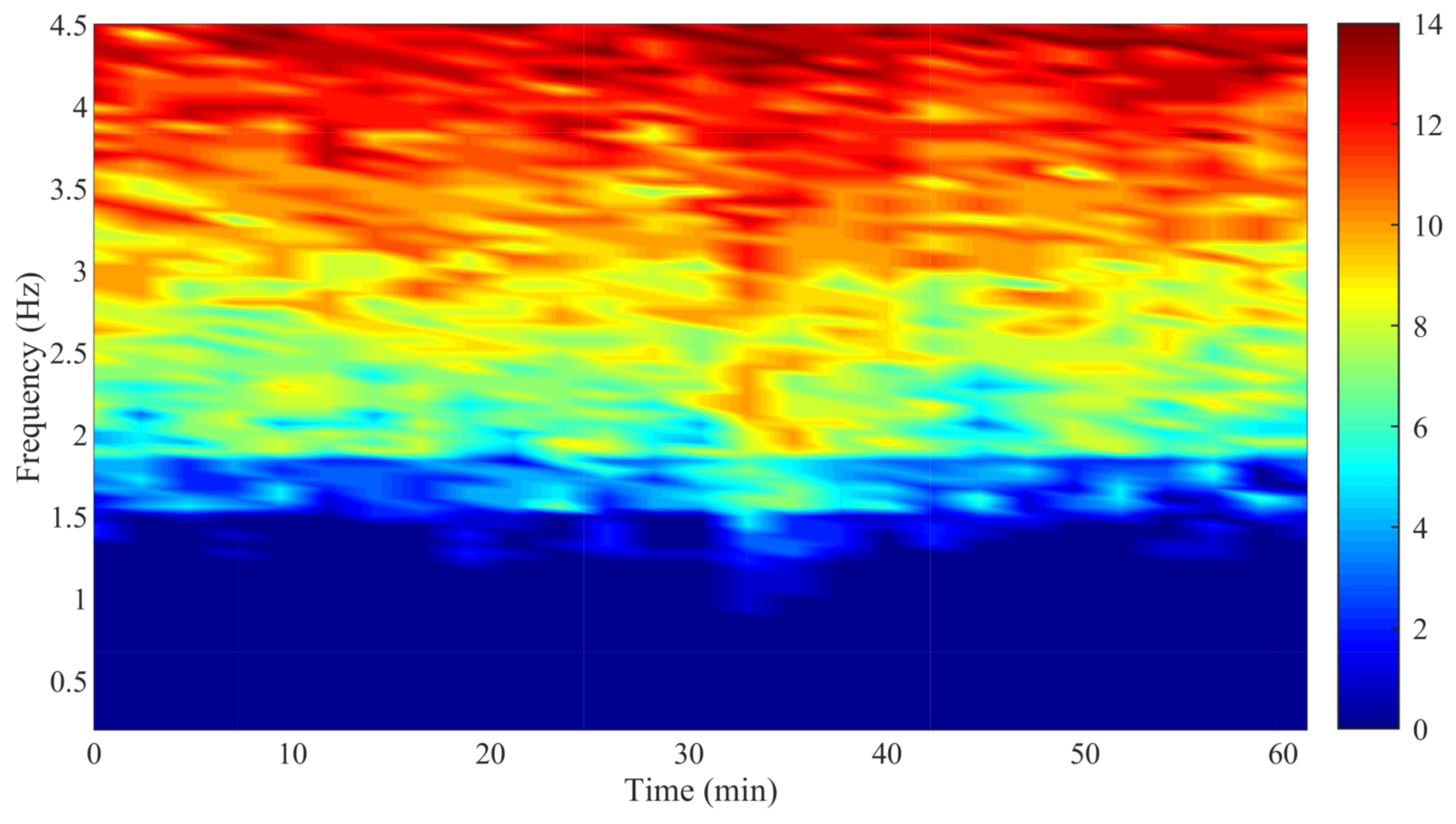
The values of basic parameters used in the AEF are displayed in Figure 6 and Figure 7. The value of N shown in Figure 6 is a function of frequency when gathers with the same shape are used and an averaged slowness of the medium 1.1 s/km is chosen. The weight w = 0.2 is used for this study. Note that K may be different for different gathers. Figure 7 displays the values of K of the gather marked in red in Figure 1. It shows increased values for larger frequencies because energetic events dominate higher frequencies over almost the entire time, as is indicated in Figure 4c. Between 30–40 min at around 1.5–3 Hz, Figure 7 shows larger values of K. It corresponds well with Figure 4a, where Event B happens at 30–40 min. For frequencies lower than 1.5 Hz, the values of K are very small, indicating a better equipartitioned wavefield for lower frequencies.

4. Shear-Wave Tomography

The dispersive behavior of the retrieved surface waves carry useful information about the subsurface. The dispersion property of the retrieved surface waves is highly sensitive to shear-wave velocities at different depths and is used to perform 3D shear-wave tomography of the area.
The slowness-frequency transform (SFT) [31] is applied to the retrieved NCC of each gather. The result of the SFT can be expressed as a Gabor diagram, which shows signal energy as a function of frequency and phase velocity. Then, the phase–velocity dispersion curves can be extracted from the resulting Gabor diagram of the SFT. Examples of the retrieved dispersion curves can be found in [22].

4.1. The ASSA Inversion

A nonlinear optimization method, adaptive simplex simulated annealing algorithm (ASSA) [32], is applied to the fundamental mode of extracted dispersion curves of all gathers for estimating shear-wave velocity as a function of depth and range in the sea bottom.
The ASSA combines the simulated annealing and downhill simplex method. It operates on a simplex of M models and randomly perturbs the parameters after a downhill simplex step. The obtained trial model is subsequently accepted or rejected according to the Metropolis criteria
P ( Δ E ) = exp ( Δ E / T ) ,
where T denotes the temperature and E denotes the mismatch. The temperature T is decreased every N p accepted perturbations using
T j = β j T 0 ,
where T 0 denotes the initial temperature and β denotes a temperature reduction factor satisfying 0 < β < 1 . The procedure continues until the models in the simplex satisfy the convergence condition
E high E low E high + E low / 2 < ϵ ,
where E high and E low represent the highest and lowest mismatch model in the simplex, respectively. Assuming that the measured dispersion data errors (including measurement error and theory error) are independent, Gaussian-distributed random processes, the likelihood function can be written as
L ( m ) = 1 ( 2 π ) N / 2 i = 1 N σ i exp i = 1 N d i d i ( m ) 2 2 σ i 2 ,
where d denotes the dispersion data vector with N entries, d ( m ) denotes the modeled data vector and σ is the standard deviation of d . The data misfit
E ( m ) = i = 1 N d i d i ( m ) 2 2 σ i 2
is used as the objective function in the inversion. Therefore, the ASSA minimizes the misfit and yields an maximum-likelihood solution.
The chosen values of the mentioned parameters in this paper are listed in Table 1. Note that M is chosen based on the dimensional of the search space, E 0 is the initial misfit of the initialized model and σ i is assumed to be the same for all entries of σ .
The forward problem is solved using the DISPER80 subroutines [33], which can calculate phase–velocity dispersion curves given a geoacoustic model.

4.2. Seabed Parameterizations

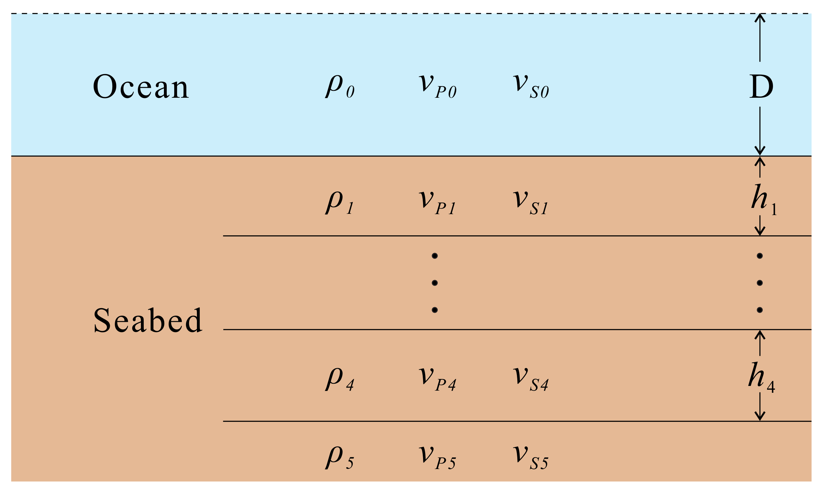
A 6-layer geoacoustic model (shown in Figure 8) is used in the inversion. The 6th layer is a semi-infinite space. Considering that the dispersion property of the surface wave is not sensitive to the density ρ and the compressional velocity v P in the frequency range used (0.2 to 4.5 Hz), we use the following empirical equation [34,35]
v P = 1.16 × v S + 1.36 ,
ρ = 1.74 v P 0.25 ,
to evaluate the values of them during the inversion.
The shear-wave velocity v S and the thickness of the layer h are variable in the iteration of the inversion process. Prior bounds are applied to the geoacoustic parameters for excluding physically unreasonable values. Table 2 shows the chosen bounds for different parameters.

4.3. Tomography Result

The ASSA provides the maximum-likelihood solution of the data. We have performed 100 independent ASSA inversions on each gather to form a mean shear-wave velocity profile. A 3D shear-wave structure (Figure 9a and Figure 10) can be reconstructed based on the solution.
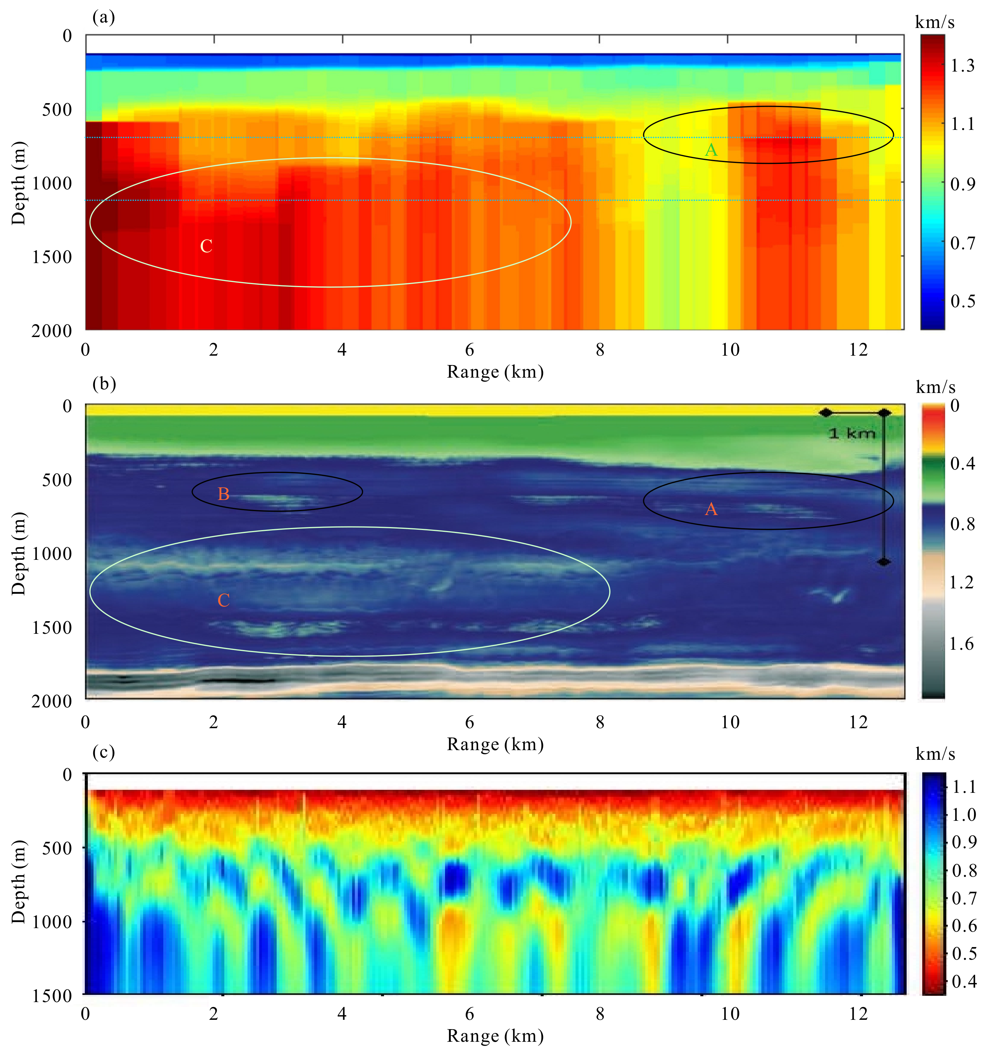
Figure 9a displays a vertical slice of the shear-wave subsurface structure under the 10th cable counted from left to right of the PRMRA in Figure 1. Four subsurface layers (excluding the water layer) are well resolved from a holistic perspective, although a 6-layer model is used in the inversion. The top white layer (0–125 m) denotes the water layer. The first layer (125–140 m) is a low-velocity layer (lower than 300 m/s) which is very thin. This layer locates near the ocean bottom and is thought to be very soft. The second layer (140–240 m) is relatively thicker and harder, and contains a velocity of about 500 to 600 m/s. As the depth goes deeper, the layers become much thicker and contain larger velocities. The third layer (240–500 m) contains a velocity of about 800 to 900 m/s. The interfaces for the top three layers below the water layer are clear and the velocity values distribute relatively homogeneous over range. The bottom layer (>500 m) is a high-velocity layer. The velocity values of it mostly span from 900 to 1300 m/s (can be even larger in several areas), indicating a more complicated structure compared with the top three layers. Note that the resolution in range of Figure 9 is 200 m, which is dependent on the chosen overlap between the adjacent gathers.
Figure 9b displays a similar slice of the shear-wave subsurface structure from active-source reflection tomography at the same field from [36]. The active-source has higher energy and the resolution of the reflection tomography is better. Thus, we consider it as a good approximation to the true model of the seabed. The top thin layer (125–140 m) of Figure 9a can not be recognized in Figure 9b. It might be caused by the regularization method which smooths the layers. However, it can be recognized easily in the P-wave velocity structure in [36]. The existence of the top thin layer in Figure 9a is reasonable because the top layer of shallow ocean is usually very soft with low shear-wave velocity. Figure 9b combines the first and second layer ( 125–240) of Figure 9a and shows a velocity of around 500 m/s at this layer. When the depth goes deeper in Figure 9b (240–500 m, corresponding to the third layer of Figure 9a), the velocity increases from 500 to 900 m/s. The third layer of Figure 9a can be considered as a transition layer at this place, compared with Figure 9b. In the depth range of 500 to 1700 m, although Figure 9a generally shows higher velocities than Figure 9b, they do have some similarities in the structure. At the depth of 600 m, Figure 9b shows two high-velocity zones A and B. We can find a similar zone A in Figure 9a, while zone B is not visible here possibly because of limited resolution of inversion using ambient noise. If we look further at the horizontal slice of the subsurface structure at the depth of 600 m in Figure 10c, both the high-velocity zones A and B can be recognized. At the depth of 1000 to 1600 m, Figure 9b shows another large high-velocity zone C. We can find a similar zone C in Figure 9a, although it is not as large as the zone in Figure 9b. The horizontal slice of Figure 9a at the depth of 1100 m demonstrates the distribution of this zone in Figure 10d, which is larger than it shows in Figure 9a. The high similarity in these zones of Figure 9a,b indicates that these high velocity anomalies are reliable and can be recognized as real features of the seabed. Below the depth of 1700 m, Figure 9b indicates a layer with very high velocities, which can not be recognized in Figure 9a. One possible reason is that surface wave can not penetrate to this depth, so that the inversion of Figure 9a is not sensitive to the shear-wave velocity at this depth.
Figure 9c displays a similar slice of the shear-wave subsurface structure from 1D Monte Carlo ambient noise tomography using 12 h of continuous ambient noise records at the same field from [37]. Although Zhang et al. [37] also did 2D and 3D tomography with the same data and obtained smoother results, Figure 9c is more comparable with the result of the present paper other than 2D and 3D results because they both use 1D parametrization. Figure 9c illustrates continuously increasing velocities from the depth of 125 to 500 m. The general structure corresponds well with Figure 9a,b. When the depth goes deeper than 500 m, Figure 9c shows complicated structure. These complicated features are thought to be artifacts due to the inversion strategy. Although lateral spatial constraints in 2D and 3D tomography make the structure smoother [37], the zones recognized in Figure 9a,b are not visible. One possible reason is that the authors used a narrower frequency band (0.35–1.5 Hz) compared with what we have used, and the information of the dispersion curves is limited. If more modes are included in the inversion, the frequency band needs to be wider. On the other side, people have to deal with the problem of the interferences included when a wider frequency band is used. At a depth deeper than 500 m, Figure 9c seems to get lower mean velocities than Figure 9a. The difference can be explained by several factors. One factor is the measurement errors of the dispersion data. The depth sensitivity (described in the following section) indicates that only lower frequency components can penetrate to a deeper depth so that the measurement errors at low frequencies may result in large bias to the velocities of deeper layers. The other factor is the large uncertainty at deeper layers caused by the inversion method, which can be quantified by statistical methods. The uncertainty for depth deeper than 500 m of Figure 9c is about 250 m/s [37] and the uncertainty for depth deeper than 500 m of Figure 9a is about 100 m/s (described in the following section).
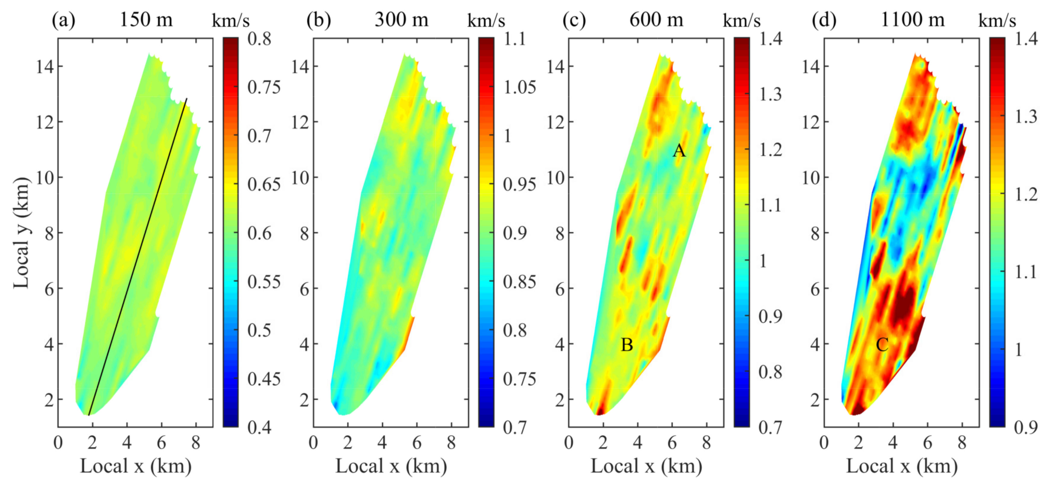
Figure 10 displays four horizontal slices of the shear-wave subsurface structure at different depths. The distribution is roughly ‘flat’ for Figure 10a,b except for some small areas with a little bit high shear-wave velocities. Figure 10c,d show the horizontal distribution of the shear-wave velocities corresponding to the straight dashed lines marked in Figure 9a. In Figure 10c, zones A and B are a little discrete. This is probably because the results slightly overfit the local data. Adding lateral constraints to the parametrization of the inversion may help to improve it. The high velocity patches in Figure 10c,d correspond to the high velocity patches in Figure 9b well. It indicates that there may be similar geological features at this field although the ground-truth is not known.

5. Discussion

5.1. Depth Sensitivity

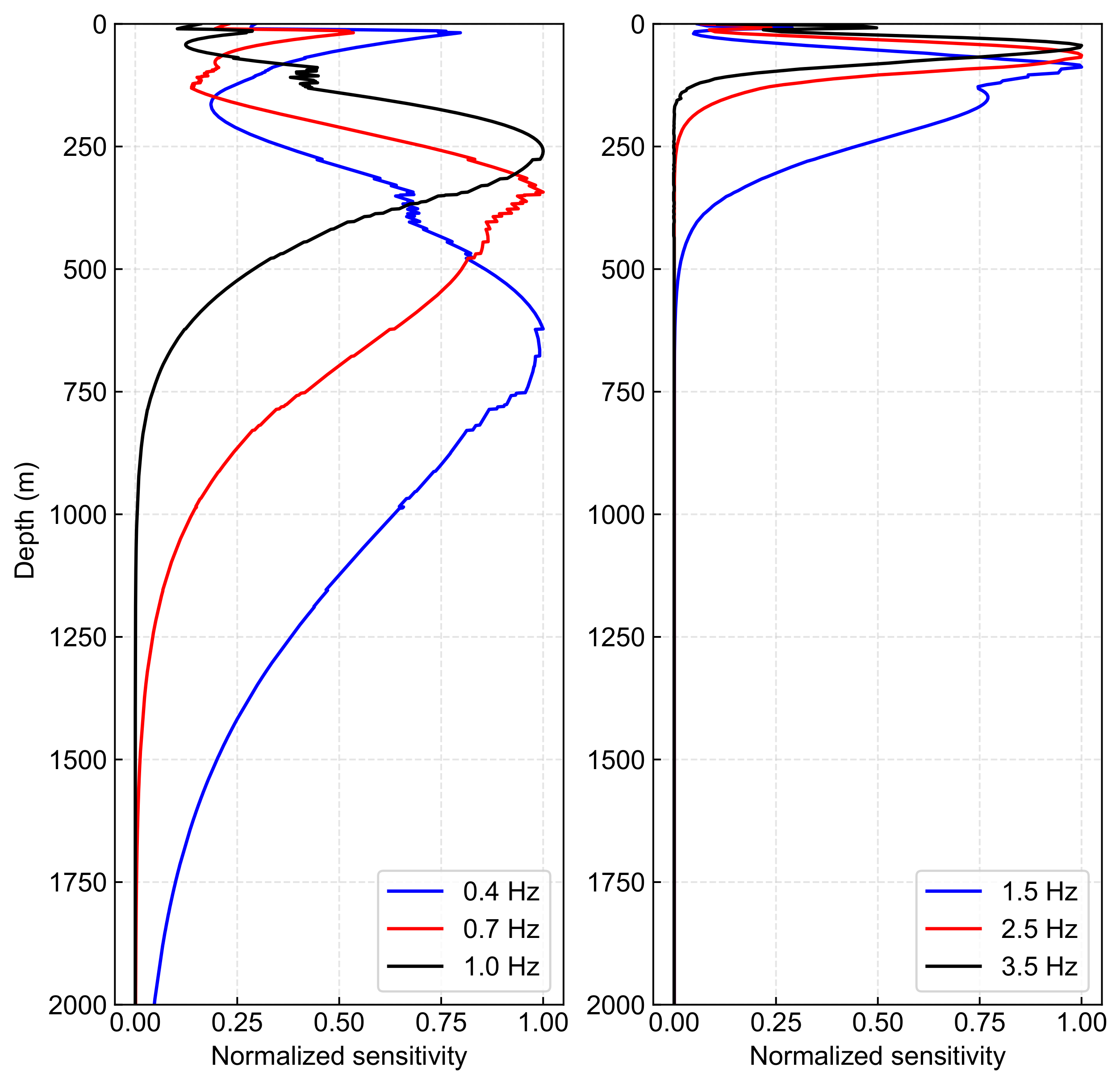
To evaluate the depth sensitivity of the inversion, we investigate the depth sensitivity kernels of the surface waves based on the inverted shear-wave velocity model. It is constructed by computing partial derivative of the predicted phase velocity with respect to velocity perturbation at different depths.
Figure 11 shows the normalized depth sensitivity kernels for different frequencies of surface waves. It shows that lower-frequency kernels have peak sensitivity at deeper depths while higher-frequency kernels have less sensitivity to deep subsurface structure. It also indicates that deeper layers may be mostly determined by frequencies lower than 1 Hz.

5.2. Tomography Resolution

The ASSA inversions are performed on 1D gathers and then all gathers are used to reconstruct the 3D shear-wave tomographic model. Since we use 30 continuously adjacent sensors (with 50 m spacing) in one cable as a gather and 25 sensors as the overlap between the adjacent gathers, the resolution along the cable is 250 m. The resolution across the cables depends on the spacing between cables, which is 300 m. The thickness of each layer is adaptive during the inversion process. Generally speaking, shallow layers have higher resolution due to the high sensitivity of both high frequencies and low frequencies of surface waves while deeper layers (>1000 m) have lower resolution since they only have some sensitivity to very low frequencies of surface waves.

5.3. Non-Uniqueness and Uncertainty

An important issue should be mentioned is that the non-uniqueness of the solution. Several factors can account for the non-uniqueness of the solution of the shear-wave inversion problem. One factor is that the problem is a highly nonlinear inverse problem and there is no analytical solution available. Numerical methods are used to solve such problems and the uniqueness of the solution to given data are not proven. Another factor is that the given data are usually noisy. In this paper, we assume that the dispersion data uncertainty are independent and Gaussian distributed (Equation (8)). In general, an infinite number of models fitting the noisy data can be found to an acceptable level [32]. The third factor is that, in practice, the dispersion curves are usually cut off to a certain frequency band or sometimes only part of the dispersion curves can be excited by the source, leading to some uncertainties to the solution.
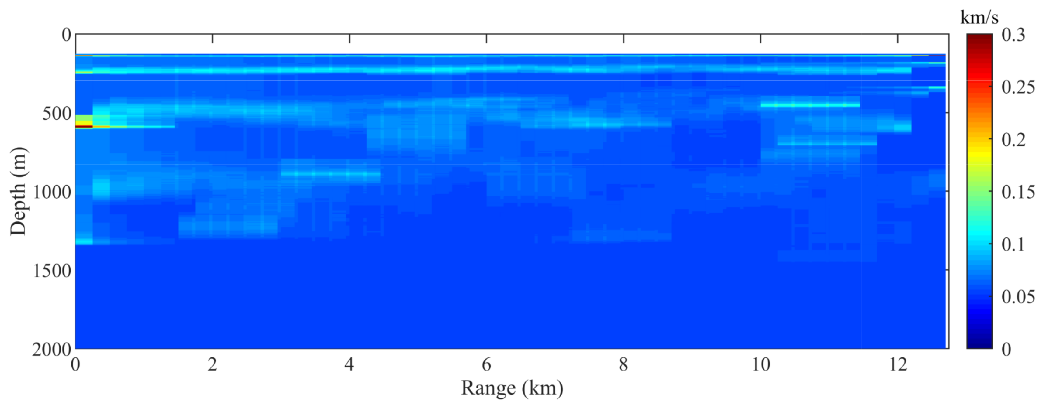
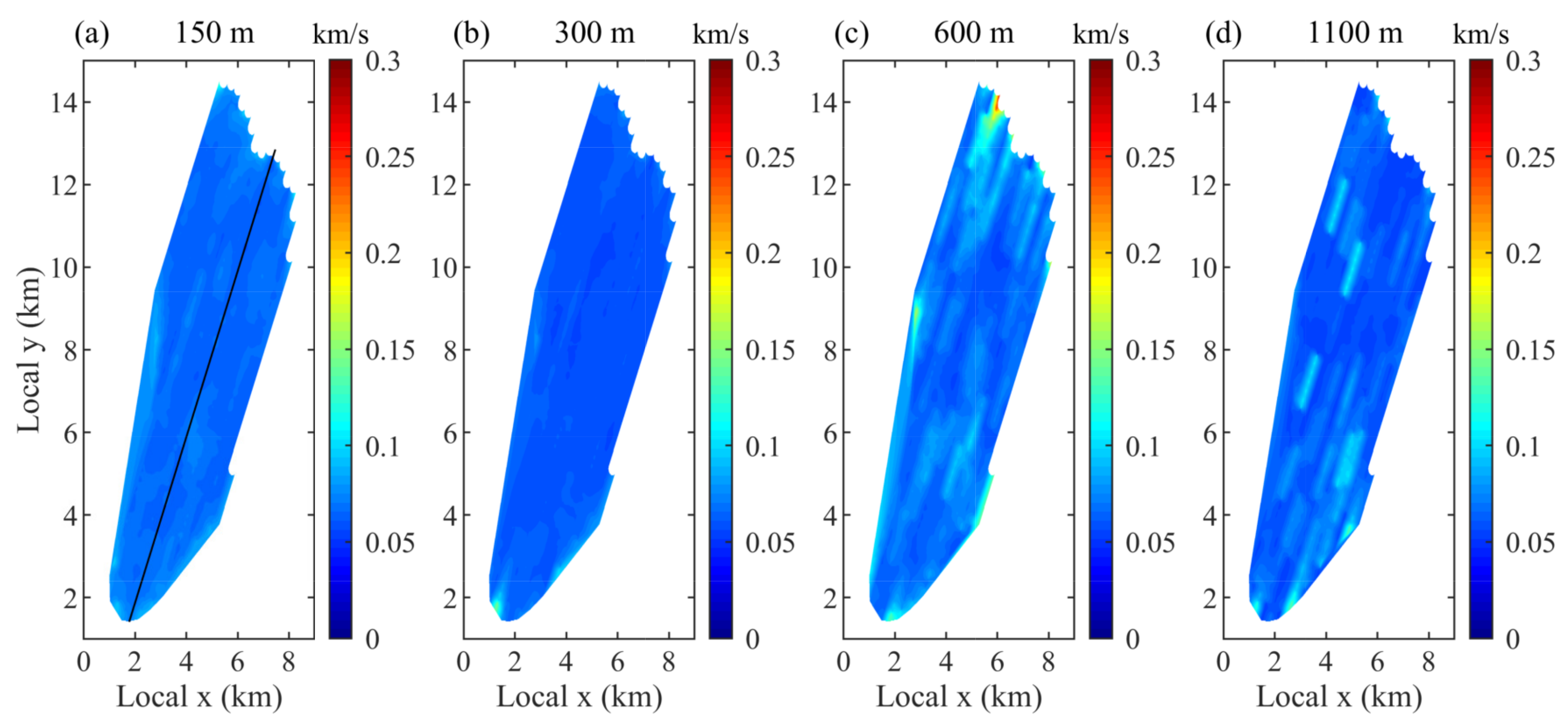
To quantify the uncertainty of the inversion, we have calculated the standard deviation of 100 independent ASSA inversions. Figure 12 and Figure 13 show a vertical and a horizontal slice of the standard deviation of the resolved shear-wave subsurface structure, respectively. Figure 12 indicates an average standard deviation of about 100 m/s. The standard deviation becomes larger at interfaces of layers and zones with a complicated structure (500 to 1500 m). This is because the thickness of each layer is adaptively determined, making slightly different layers for each independent inversion and resulting in larger standard deviation at the interfaces. Figure 13 indicates a generally homogeneous standard deviation on horizontal slices. The uncertainty for deeper layers is not as large as Zhang et al. [37] because our parameterization on number of layers and larger thickness of deeper layers, which constrains the freedom and uncertainty although limiting the resolution at the same time.

6. Conclusions

Shear-wave tomography is performed using only 1.02-h ambient noise recorded by a permanent reservoir monitoring receiver array installed in the Norwegian North Sea. Passive tomography needs the wavefield to be diffuse and equipartitioned. However, the wavefield can usually be contaminated by various events in the real world. Time and frequency analysis indicates that the ambient noise used in the paper is contaminated by several high energy events. The beamforming results further clarify that these events are directional and should be suppressed before the noise is cross-correlated. An adapted eigenvalue-based filter is applied to accomplish the suppression and shows good effects both in beamforming and noise crosscorrelation results. The filter makes it possible to implement shear-wave tomography on the ambient noise with interference. Finally, an adaptive simplex simulated annealing algorithm (ASSA) is applied for estimating the three-dimensional subsurface shear-wave structure. The results indicate a four-layer structure with a generally increasing velocity as the depth goes deeper. The velocity values of the first three layers distribute relatively homogeneous, while the fourth layer shows a more complicated distribution, indicating a heterogeneous structure under 500 m. The comparison of the tomography result with other methods demonstrates that the tomography presented in this paper is reasonable and encouraging, although the ambient noise is very short and contaminated.

Author Contributions

Formal analysis, G.W., H.D., G.K., and J.S.; Funding acquisition, H.D. and J.S.; Methodology, G.W. and H.D.; Resources, G.W. and G.K.; Software, G.W. and H.D.; Writing—original draft, G.W.; Writing—review and editing, H.D., G.K., and J.S. All authors have read and agreed to the published version of the manuscript.

Funding

This research was funded by the National Natural Science Foundation of China, Grant Number [41605070].

Acknowledgments

The authors would like to acknowledge Grane license partners (Equinor ASA, Petoro AS, Vår Energi AS, and ConocoPhillips Skandinavia AS) for allowing to present this work. The views and opinions expressed in this paper are those of the authors and are not necessarily shared by the license partners; H.D. thanks the Norwegian Research Council and the industry partners of the GAMES consortium at NTNU for financial support (Grant No. 294404); We would like to give special thanks to section managing editor Bommie Xiong and unknown reviewers for their help and comments that significantly improved the manuscript.

Conflicts of Interest

The authors declare no conflict of interest.

Abbreviations

The following abbreviations are used in this manuscript:
PSIPassive seismic interferometry
NCCNoise crosscorrelations
1D/2D/3D1/2/3 dimensional
PRMRAPermanent reservoir monitoring receiver array
SCMSample covariance matrix
ASSAAdaptive simplex simulated annealing algorithm

Appendix A. The Strategies to Determine N and K

This appendix provides the strategies we follow to determine the value of N and K. The strategies are from [22] and a more complete description can be found there.

Appendix A.1. The Determination of N

Supposing that γ is the slowness of the medium, f is the frequency, N is the number of sensors, r i j is the great-circle distance between two sensors i and j, and r ¯ is the typical separation of the array which is defined as
r ¯ = 2 N ( N 1 ) i = 1 N j > i N r i j ,
we can determine the value of N using
N ( f ) = m i n { 2 2 π f γ r ¯ + 1 , N / 2 } ,
where x is the least integer greater than or equal to x.
Equation (A2) implies that the determination of N only relies on the frequency, the slowness of the medium, the typical separation, and the number of sensors used. Since the slowness of the medium is not known beforehand, a rough estimation of the average slowness is sufficient to use in practice, as is suggested by Seydoux et al. [30] (1.1 s/km is used in this paper). Thus, if we choose gathers with the same shapes, the value of N is a function of frequency.

Appendix A.2. The Determination of K

A statistical hypothesis test is used to determine K. At each frequency f, the eigenvalues { λ ^ 1 , , λ ^ N 1 } of R ^ are tested sequentially at each step k using the statistic
τ ( k ) = λ ^ k σ ¯ k ,
with
σ ¯ k = i = k N λ ^ i N k + 1 .
Note that τ ( k ) relies on the local noise characteristics of the chosen gather and may be different across gathers. The tested eigenvalue λ ^ k is rejected and suppressed to an average level at a significance level α if
τ ( k ) > w P m a x | R ^ c N k + 1 1 ( 1 α ) ,
where P m a x | R ^ c N k + 1 is the empirical cumulative distribution of the largest eigenvalue of an N k + 1 dimensional SCM R ^ c N k + 1 , which can be pre-computed by 1000 Monte Carlo trials. The significance level α = 0.05 is usually used. The weight w satisfies 0 w 1 and is used to affect the selection of K. A weight selection study [22] can be referred to choose an appropriate value for the weight. When the test stops rejecting, the value k is used as K. The statistical model of the SCM R c ^ relating to a diffuse noise field is simulated using
R ^ c = 1 M R c X X H ,
where X is an N × M random matrix with entries X i j ~ C N ( 0 , 1 ) , and R c is the analytical covariance matrix of isotropic noise field defined as
[ R c ] i j = J 0 ( 2 π f γ r i r j ) ,
in which J 0 is the zeroth order Bessel function of the first kind, and r i denotes the position of the receiver i. Similarly, an estimation of the average slowness is sufficient to use in practice (1.1 s/km is used in this paper). Note that, if we choose gathers with the same shapes, the value of R c is a function of frequency.
Considering these formulas from Equations (A3)–(A7), we can find that the determination of K not only relies on the frequency but also on local noise characteristics of the chosen gathers.

References

  1. Campillo, M.; Paul, A. Long-range correlations in the diffuse seismic coda. Science 2003, 299, 547–549. [Google Scholar] [CrossRef] [PubMed] [Green Version]
  2. Wapenaar, K. Retrieving the elastodynamic Green’s function of an arbitrary inhomogeneous medium by cross correlation. Phys. Rev. Lett. 2004, 93, 254301. [Google Scholar] [CrossRef] [PubMed] [Green Version]
  3. Draganov, D.; Wapenaar, K.; Thorbecke, J. Seismic interferometry: Reconstructing the earth’s reflection response. Geophysics 2006, 71, SI61–SI70. [Google Scholar] [CrossRef] [Green Version]
  4. De Ridder, S.; Biondi, B. Daily reservoir-scale subsurface monitoring using ambient seismic noise. Geophys. Res. Lett. 2013, 40, 2969–2974. [Google Scholar] [CrossRef]
  5. Obermann, A.; Froment, B.; Campillo, M.; Larose, E.; Planes, T.; Valette, B.; Chen, J.; Liu, Q. Seismic noise correlations to image structural and mechanical changes associated with the Mw 7.9 2008 Wenchuan earthquake. J. Geophys. Res. Solid Earth 2014, 119, 3155–3168. [Google Scholar] [CrossRef]
  6. Obermann, A.; Kraft, T.; Larose, E.; Wiemer, S. Potential of ambient seismic noise techniques to monitor the St. Gallen geothermal site (Switzerland). J. Geophys. Res. Solid Earth 2015, 120, 4301–4316. [Google Scholar] [CrossRef]
  7. Aki, K. Space and time spectra of stationary stochastic waves, with special reference to microtremors. Bull. Earthq. Res. Inst. 1957, 35, 415–456. [Google Scholar]
  8. Claerbout, J.F. Synthesis of a layered medium from its acoustic transmission response. Geophysics 1968, 33, 264–269. [Google Scholar] [CrossRef]
  9. Weaver, R.L.; Lobkis, O.I. Ultrasonics without a source: Thermal fluctuation correlations at MHz frequencies. Phys. Rev. Lett. 2001, 87, 134301. [Google Scholar] [CrossRef]
  10. Weaver, R.L.; Lobkis, O.I. On the emergence of the Green’s function in the correlations of a diffuse field. J. Acoust. Soc. Am. 2001, 110, 3011–3017. [Google Scholar] [CrossRef]
  11. Derode, A.; Larose, E.; Tanter, M.; De Rosny, J.; Tourin, A.; Campillo, M.; Fink, M. Recovering the Green’s function from field-field correlations in an open scattering medium (L). J. Acoust. Soc. Am. 2003, 113, 2973–2976. [Google Scholar] [CrossRef] [PubMed]
  12. Wapenaar, K. Synthesis of an inhomogeneous medium from its acoustic transmission response. Geophysics 2003, 68, 1756–1759. [Google Scholar] [CrossRef] [Green Version]
  13. Roux, P.; Sabra, K.G.; Kuperman, W.A.; Roux, A. Ambient noise cross correlation in free space: Theoretical approach. J. Acoust. Soc. Am. 2005, 117, 79–84. [Google Scholar] [CrossRef] [PubMed] [Green Version]
  14. Rickett, J.; Claerbout, J. Acoustic daylight imaging via spectral factorization: Helioseismology and reservoir monitoring. Lead. Edge 1999, 18, 957–960. [Google Scholar] [CrossRef] [Green Version]
  15. Roux, P.; Fink, M. Green’s function estimation using secondary sources in a shallow water environment. J. Acoust. Soc. Am. 2003, 113, 1406–1416. [Google Scholar] [CrossRef]
  16. Stehly, L.; Fry, B.; Campillo, M.; Shapiro, N.; Guilbert, J.; Boschi, L.; Giardini, D. Tomography of the Alpine region from observations of seismic ambient noise. Geophys. J. Int. 2009, 178, 338–350. [Google Scholar] [CrossRef] [Green Version]
  17. Pilz, M.; Parolai, S.; Bindi, D. Three-dimensional passive imaging of complex seismic fault systems: Evidence of surface traces of the Issyk-Ata fault (Kyrgyzstan). Geophys. J. Int. 2013, 194, 1955–1965. [Google Scholar] [CrossRef] [Green Version]
  18. Mordret, A.; Landès, M.; Shapiro, N.; Singh, S.; Roux, P. Ambient noise surface wave tomography to determine the shallow shear velocity structure at Valhall: Depth inversion with a Neighbourhood Algorithm. Geophys. J. Int. 2014, 198, 1514–1525. [Google Scholar] [CrossRef] [Green Version]
  19. Galetti, E.; Curtis, A.; Baptie, B.; Jenkins, D.; Nicolson, H. Transdimensional Love-wave tomography of the British Isles and shear-velocity structure of the East Irish Sea Basin from ambient-noise interferometry. Geophys. J. Int. 2016, 208, 36–58. [Google Scholar] [CrossRef]
  20. Wang, Y.; Lin, F.C.; Schmandt, B.; Farrell, J. Ambient noise tomography across Mount St. Helens using a dense seismic array. J. Geophys. Res. Solid Earth 2017, 122, 4492–4508. [Google Scholar] [CrossRef]
  21. Weaver, R.L. Equipartition and retrieval of Green’s function. Earthq. Sci. 2010, 23, 397–402. [Google Scholar] [CrossRef] [Green Version]
  22. Wu, G.; Dong, H.; Ke, G.; Song, J. An adapted eigenvalue-based filter for ocean ambient noise processing. Geophysics 2019, 85, KS29–KS38. [Google Scholar] [CrossRef]
  23. Tsai, V.C. On establishing the accuracy of noise tomography travel-time measurements in a realistic medium. Geophys. J. Int. 2009, 178, 1555–1564. [Google Scholar] [CrossRef] [Green Version]
  24. Tsai, V.C. Understanding the amplitudes of noise correlation measurements. J. Geophys. Res. Solid Earth 2011, 116, B09311. [Google Scholar] [CrossRef] [Green Version]
  25. Froment, B.; Campillo, M.; Roux, P.; Gouedard, P.; Verdel, A.; Weaver, R.L. Estimation of the effect of nonisotropically distributed energy on the apparent arrival time in correlations. Geophysics 2010, 75, SA85–SA93. [Google Scholar] [CrossRef] [Green Version]
  26. Fichtner, A. Source and processing effects on noise correlations. Geophys. J. Int. 2014, 197, 1527–1531. [Google Scholar] [CrossRef] [Green Version]
  27. Fichtner, A.; Stehly, L.; Ermert, L.; Boehm, C. Generalised interferometry-I: Theory for inter-station correlations. Geophys. J. Int. 2016, 208, 603–638. [Google Scholar] [CrossRef]
  28. Olofsson, B. Marine ambient seismic noise in the frequency range 1–10 Hz. Lead. Edge 2010, 29, 418–435. [Google Scholar] [CrossRef]
  29. Kim, J.; Choi, H. Response modification factors of chevron-braced frames. Eng. Struct. 2005, 27, 285–300. [Google Scholar] [CrossRef]
  30. Seydoux, L.; de Rosny, J.; Shapiro, N.M. Pre-processing ambient noise cross-correlations with equalizing the covariance matrix eigenspectrum. Geophys. J. Int. 2017, 210, 1432–1449. [Google Scholar] [CrossRef]
  31. McMechan, G.A.; Yedlin, M.J. Analysis of dispersive waves by wave field transformation. Geophysics 1981, 46, 869–874. [Google Scholar] [CrossRef]
  32. Dosso, S.; Wilmut, M.; Lapinski, A.L. An adaptive-hybrid algorithm for geoacoustic inversion. IEEE J. Ocean. Eng. 2001, 26, 324–336. [Google Scholar] [CrossRef]
  33. Saito, M. DISPER80: A subroutine package for the calculation of seismic normal mode solutions. In Seismological Algorithms; Cinii: Tokyo, Japan, 1980; pp. 293–319. [Google Scholar]
  34. Castagna, J.P.; Batzle, M.L.; Eastwood, R.L. Relationships between compressional-wave and shear-wave velocities in clastic silicate rocks. Geophysics 1985, 50, 571–581. [Google Scholar] [CrossRef]
  35. Brocher, T.M. Empirical Relations between Elastic Wavespeeds and Density in the Earth’s Crust. Bull. Seismol. Soc. Am. 2005, 95, 2081–2092. [Google Scholar] [CrossRef]
  36. Hicks, E.; Hoeber, H.; Houbiers, M.; Lescoffit, S.P.; Ratcliffe, A.; Vinje, V. Time-lapse full-waveform inversion as a reservoir-monitoring tool—A North Sea case study. Lead. Edge 2016, 35, 850–858. [Google Scholar] [CrossRef] [Green Version]
  37. Zhang, X.; Hansteen, F.; Curtis, A. Fully 3D Monte Carlo Ambient Noise Tomography over Grane Field. In Proceedings of the 81st EAGE Conference and Exhibition 2019, London, UK, 3–6 June 2019; Volume 2019, pp. 1–5. [Google Scholar]
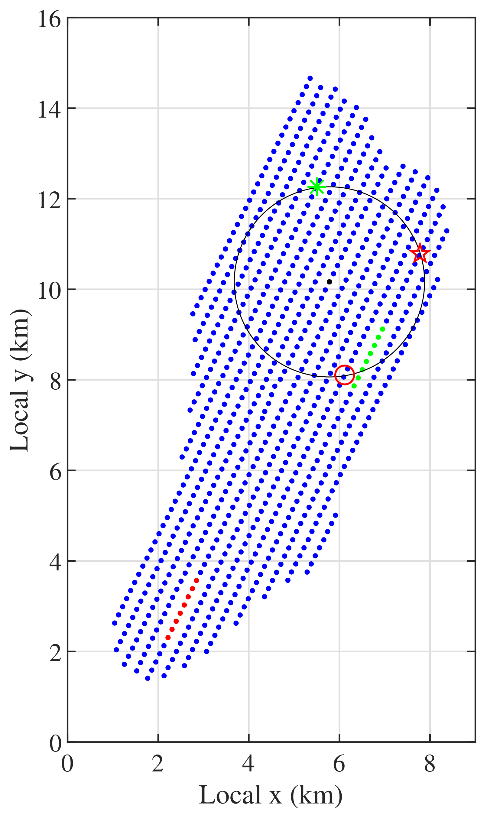
Figure 1. The PRMRA geometry. Not all the receivers are plotted in the figure for display purposes. The gather marked in red is used in the following example of beamforming. The gathers marked in green and red are used in the following examples of the NCC retrieval. The black circle and marks on it are used in the following study of events.
Remotesensing 12 02969 g001
Figure 2. Temporal and spectral analysis. Letters A, B and C denote different events detected. (a) the pressure recorded at one receiver. The pressure is normalized by the maximum amplitude. The blue box selects a window where the noise is not affected by severe events. The green box selects a window where the noise is affected by Event A. The red box selects a window where the noise is affected by Event B; (b) the averaged PSD (dB re 1 Pa2/Hz) of all receivers as a function of time and frequency (spectrogram); (c) the enlarged view of the noise marked by blue box in (a); (d) the PSD of the corresponding noise marked by boxes in (a). The curves are related to the noise by the color of the boxes in (a). The black curve is the averaged PSD over 60 min.
Remotesensing 12 02969 g002
Figure 3. (a) arrival analysis on Event A. The green waveform represents the earliest arrival and the red waveform represents the latest arrival. The amplitudes of the signals are normalized by the maximum of each waveform; (b) the spectrum of Event A. Note that the magnitude is normalized to the maximum value.
Remotesensing 12 02969 g003
Figure 4. Beamforming results. (a,b) show the beamforming energy distribution of 2 Hz; (c,d) show the beamforming energy distribution of 4 Hz; (a,c) show the beamforming energy distribution of the original wavefield; (b,d) show the beamforming energy distribution of the filtered wavefield using the adapted eigenvalue-based filter.
Remotesensing 12 02969 g004
Figure 5. The NCC results. Note that the NCCs are bandpass filtered between 0.2 and 4.5 Hz. (a,b) displays the NCC of the gather marked in red in Figure 1; (c,d) displays the NCC of the gather marked in green in Figure 1; (a,c) displays the NCC retrieved from unfiltered SCM while (b,d) displays the NCC retrieved from the filtered SCM.
Remotesensing 12 02969 g005
Figure 6. The value of N as a function of frequency.
Remotesensing 12 02969 g006
Figure 7. The value of K as a function of frequency and time. The chosen gather is marked in red in Figure 1.
Remotesensing 12 02969 g007
Figure 8. Geoacoustic model used in the inversion.
Remotesensing 12 02969 g008
Figure 9. (a) a vertical slice of the resolved mean shear-wave subsurface structure under the 10th cable counted from left to right of the PRMRA in Figure 1. The top white layer represents the water layer. The dashed lines indicate the horizontal slices used in Figure 10; (b) a vertical slice of the shear-wave subsurface structure from active-source reflection tomography [36]; (c) a vertical slice of the shear-wave subsurface structure from 1D Monte Carlo ambient noise tomography [37]. The circles in (a,b) mark the high-velocity zones.
Remotesensing 12 02969 g009
Figure 10. (ad) show horizontal slices of the mean shear-wave subsurface structure at the depth of 150, 300, 600 and 1100 m, respectively. The black line in (a) shows the location of Figure 9. The letters in (c,d) correspond to the letters in Figure 9.
Remotesensing 12 02969 g010
Figure 11. Normalized depth sensitivity kernels for different frequencies of surface waves.
Remotesensing 12 02969 g011
Figure 12. A vertical slice of the standard deviation of the resolved shear-wave subsurface structure under the 10th cable counted from left to right of the PRMRA in Figure 1.
Remotesensing 12 02969 g012
Figure 13. (ad) show horizontal slices of the standard deviation of the shear-wave subsurface structure at the depth of 150, 300, 600 and 1100 m, respectively. The black line in (a) shows the location of Figure 12.
Remotesensing 12 02969 g013
Table 1. Values of the parameters used in the ASSA inversion.
ParameterDescriptionValue
MNumber of models in the simplex11
T 0 Initial temperature E 0
N p Temperature decrease frequency10
β Temperature reduction factor0.995
ϵ Convergence tolerance0.001
σ i Standard deviation of data (km/s)0.1
Table 2. Search bound of seabed parameters.
ParameterBound (km/s)ParameterBound (km)
v S 1 [0.1, 0.5] h 1 [0.01, 0.10]
v S 2 [0.2, 1.0] h 2 [0.05, 0.80]
v S 3 [0.3, 2.0] h 3 [0.10, 0.80]
v S 4 [0.3, 2.0] h 4 [0.20, 0.80]
v S 5 [0.3, 2.0] h 5 semi-infinite
v S 0 0D0.125
v P 0 1.49