Article

Comparing the Spatial Accuracy of Digital Surface Models from Four Unoccupied Aerial Systems: Photogrammetry Versus LiDAR

by
Stephanie R. Rogers
1,*,
Ian Manning
2 and
William Livingstone
2
1
Department of Geosciences, Auburn University, Auburn, AL 36849, USA
2
Applied Research, Nova Scotia Community College, Lawrencetown, NS B0S 1M0, Canada
*
Author to whom correspondence should be addressed.
Remote Sens. 2020, 12(17), 2806; https://doi.org/10.3390/rs12172806
Submission received: 30 July 2020 / Revised: 23 August 2020 / Accepted: 27 August 2020 / Published: 29 August 2020
(This article belongs to the Special Issue She Maps)

Abstract

:
The technological growth and accessibility of Unoccupied Aerial Systems (UAS) have revolutionized the way geographic data are collected. Digital Surface Models (DSMs) are an integral component of geospatial analyses and are now easily produced at a high resolution from UAS images and photogrammetric software. Systematic testing is required to understand the strengths and weaknesses of DSMs produced from various UAS. Thus, in this study, we used photogrammetry to create DSMs using four UAS (DJI Inspire 1, DJI Phantom 4 Pro, DJI Mavic Pro, and DJI Matrice 210) to test the overall accuracy of DSM outputs across a mixed land cover study area. The accuracy and spatial variability of these DSMs were determined by comparing them to (1) 12 high-precision GPS targets (checkpoints) in the field, and (2) a DSM created from Light Detection and Ranging (LiDAR) (Velodyne VLP-16 Puck Lite) on a fifth UAS, a DJI Matrice 600 Pro. Data were collected on July 20, 2018 over a site with mixed land cover near Middleton, NS, Canada. The study site comprised an area of eight hectares (~20 acres) with land cover types including forest, vines, dirt road, bare soil, long grass, and mowed grass. The LiDAR point cloud was used to create a 0.10 m DSM which had an overall Root Mean Square Error (RMSE) accuracy of ±0.04 m compared to 12 checkpoints spread throughout the study area. UAS were flown three times each and DSMs were created with the use of Ground Control Points (GCPs), also at 0.10 m resolution. The overall RMSE values of UAS DSMs ranged from ±0.03 to ±0.06 m compared to 12 checkpoints. Next, DSMs of Difference (DoDs) compared UAS DSMs to the LiDAR DSM, with results ranging from ±1.97 m to ±2.09 m overall. Upon further investigation over respective land covers, high discrepancies occurred over vegetated terrain and in areas outside the extent of GCPs. This indicated LiDAR’s superiority in mapping complex vegetation surfaces and stressed the importance of a complete GCP network spanning the entirety of the study area. While UAS DSMs and LiDAR DSM were of comparable high quality when evaluated based on checkpoints, further examination of the DoDs exposed critical discrepancies across the study site, namely in vegetated areas. Each of the four test UAS performed consistently well, with P4P as the clear front runner in overall ranking.

1. Introduction

Digital Elevation Models (DEMs) are geometric representations of the topography where elevations are represented as pixels in raster format [1]. DEMs are categorized into Digital Terrain Models (DTMs), which represent topography void of surface features; and Digital Surface Models (DSMs), which depict the top surfaces of features elevated above the earth, including buildings, trees, and towers (Figure 1). Historically, DEMs were arduously produced from surveyed field data, contour lines on topographic maps, and photogrammetry from aerial photography [2,3]. DEM accuracy and production efficiency greatly improved with the onset of Light Detection and Ranging (LiDAR). LiDAR data are costly to obtain for small areas, as they are collected from piloted aircraft (airborne LiDAR) and/or from ground level (terrestrial LiDAR). Airborne LiDAR is more efficient for regional scale studies, while terrestrial LiDAR is optimal for hyperlocal scales [4]. Additionally, both require extensive expertise in data acquisition and processing. Although LiDAR has produced some of the most accurate representations of the Earth’s surface, its availability and accessibility are technically, or financially, challenging for sections of the user group. However, the recent push towards making state-funded LiDAR data more readily available through online portals [5,6,7] will improve availability. Additionally, the technological growth and accessibility of Unoccupied Aerial Systems (UAS) have revolutionized the production of geographic information [8,9], furthering collection availability of high-resolution imagery that can be processed to create orthophotomosaics and DEMs. DEMs are input layers in many Geographic Information System (GIS) calculations and applications. DSMs, specifically, are a critical component of geospatial analyses, ranging from precision agriculture [10] to urban development [11,12], forestry [13], and 3D modeling [14].
UAS technology, in combination with photogrammetric software (e.g., Agisoft Metashape [16] and Pix4D Mapper [17]), has transformed the spatial and temporal scales at which we are able to collect information about the terrain. UAS with Red Green Blue (RGB) camera sensors have proven to be effective tools for creating high-resolution DEMs [18]. As LiDAR can penetrate through vegetation, it has the ability to collect data representing the ground, often referred to as a “bare earth model”, or DTM [19]. Due to its multiple returns, LiDAR is also used to produce DSMs. On the other hand, it is more challenging to create DTMs from UAS imagery due to the inability of the camera sensor to penetrate through canopy, thus UAS surveys are predominantly used to produce DSMs. However, advancements in Structure-from-Motion (SfM) algorithms and Dense-Image-Matching (DIM) techniques show that DTM production from UAS imagery is becoming more feasible [20,21]. The creation of DSMs from UAS imagery is facilitated through SfM algorithms, which reconstruct 3D surfaces from multiple overlapping images [22], and dense point cloud generation, or DIM, techniques. SfM has been well described in the literature [22,23], and Pricope et al. [24] provide an overview of how it is used to process UAS imagery. DIM algorithms continue to advance [25,26,27] to enable finer-resolution DSM production from UAS imagery, comparable to the level of airborne LiDAR in some environments [19,28]. Studies have shown that UAS imagery has produced comparable outputs to airborne LiDAR in various environmental settings. Gašparović et al. [29] compared UAS-based DSMs with and without Ground Control Points (GCPs) to airborne LiDAR in non-optimal weather conditions in a forestry setting. They confirmed high vertical agreement between datasets when GCPs were used and stress the importance of GCP use for accurate DSM production, as reiterated in other studies [30,31,32,33]. Wallace et al. [34] compared UAS imagery to airborne LiDAR to assess forest structure. They discovered that while UAS DSMs were not as accurate as DSMs produced from airborne LiDAR, they were a sufficient low-cost alternative for surveying forest stands but lacked detail compared to LiDAR products. Because of these advancements in UAS technology, sensors, and processing techniques, geographic data can be collected at lower altitudes, higher resolutions, and user-defined spatial and temporal scales. Thus, many researchers are testing the practical applications of these capabilities [35].
Flight control and stabilization systems, through the integration of Global Navigation Satellite System (GNSS) receivers and Inertial Measurement Units (IMUs), have facilitated the addition of LiDAR sensors on UAS. This can be more cost efficient than traditional airborne LiDAR for local-scale investigations. In recent years, UAS-LiDAR has been tested in a multitude of fields including ecology [36], forestry [37,38,39,40] and precision agriculture [41], predominantly for vegetation mapping [42]. Results in each case showed that UAS-LiDAR produced high-quality, reliable results when compared to airborne LiDAR sources. Several different LiDAR models are available for use on UAS and are introduced in the study by Giordan et al. [42]. Here, we focus on the Velodyne VLP-16 Puck Lite model, which was common at the time of data collection.
In this study, we use photogrammetry and high-precision GCPs to create DSMs from four popular UAS (DJI Inspire 1, DJI Phantom 4 Pro, DJI Mavic Pro, and DJI Matrice 210) to compare the results of commonly purchased platforms. The accuracy and spatial variability of these DSMs will be compared to (1) 12 high-precision GPS targets (checkpoints) in the field to quantify overall vertical accuracy, and (2) a DSM created from Light Detection and Ranging (LiDAR) (Velodyne VLP-16 Puck Lite) on a fifth UAS, a DJI Matrice 600 Pro, to investigate spatial errors across the study area. This research was designed to quantify how DSMs generated from multiple UAS differ, and to identify and characterize differences across space and land cover types in a single study area.

2. Materials and Methods
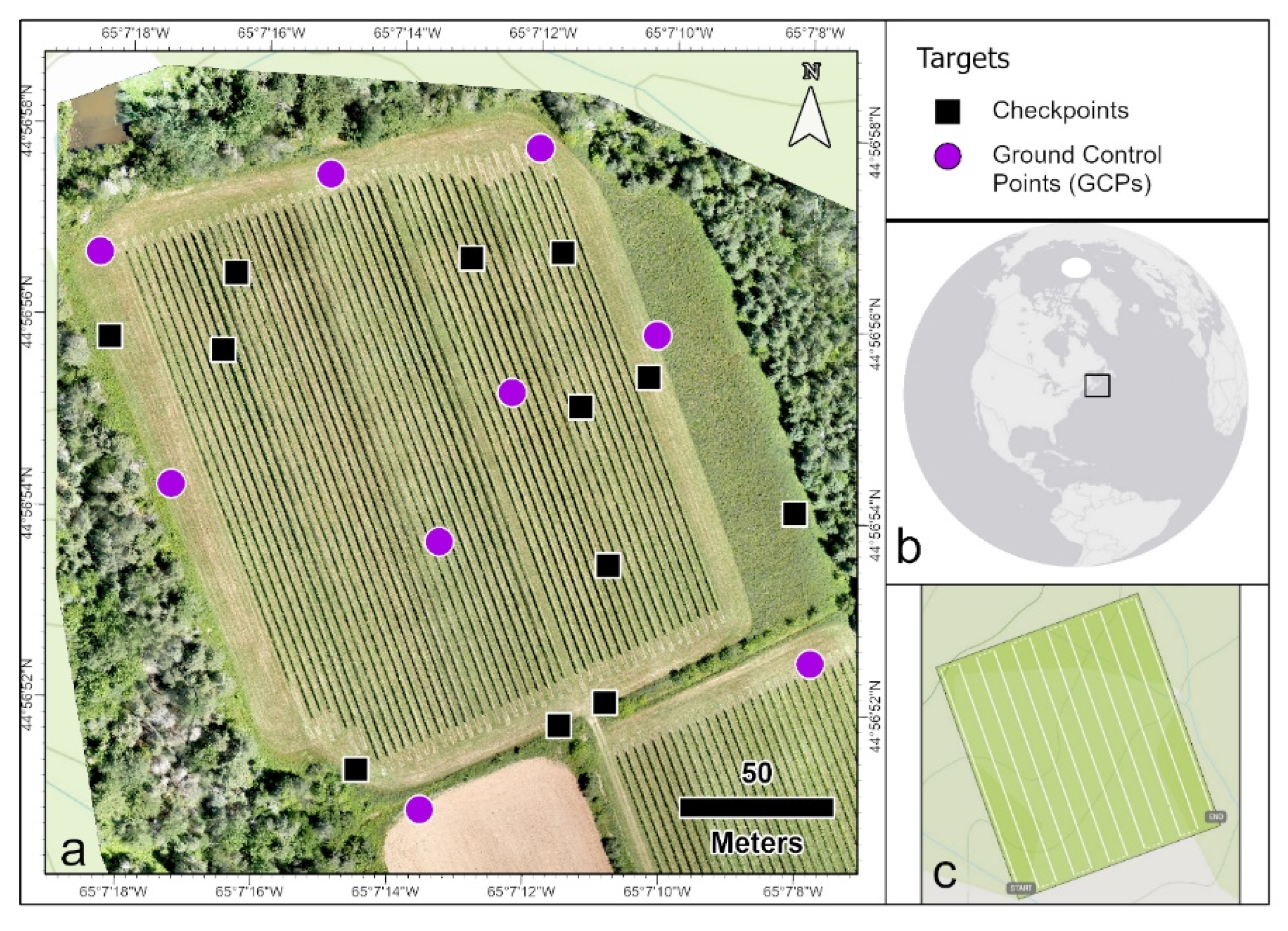
2.1. Study Site

The study site, located at 44°56′55″N, 65°07′13″W near Middleton, Nova Scotia (NS), Canada (Figure 2), was chosen due to its mixed land cover features, including vines, bare soil, dirt road, long grass, mowed grass, and forest. The site was approximately eight hectares (~20 acres) in area which enabled each flight to be conducted on a single battery (approximately 15 min flying time).

2.2. Ground Control Points (GCPs) and Checkpoints

Twenty-one (21) targets were spread across the study area (Figure 2); nine Aeropoint™ targets with integrated GPS were used as GCPs for georectifying the UAS imagery (Section 2.5). Additionally, 12 checkpoints in the form of 2′ × 2′ wooden targets, painted in a black-and-white checkerboard pattern, were spread across the study area. The Aeropoint targets were used to reference the model (GCPs) and the remaining targets were retained for validating model accuracy (checkpoints). The location of each target was logged using a Leica RTK GPS 1200 survey-grade GNSS receiver (1 cm accuracy). All GPS data were post-processed using data from the Nova Scotia Active Control System station (NSACS) number NS250002 [43] in Lawrencetown, NS, which was approximately eight kilometers away from the study site. Locations of Aeropoint targets were processed using the Aeropoints cloud-based system and Leica GPS locations were post-processed using Leica GeoOffice.

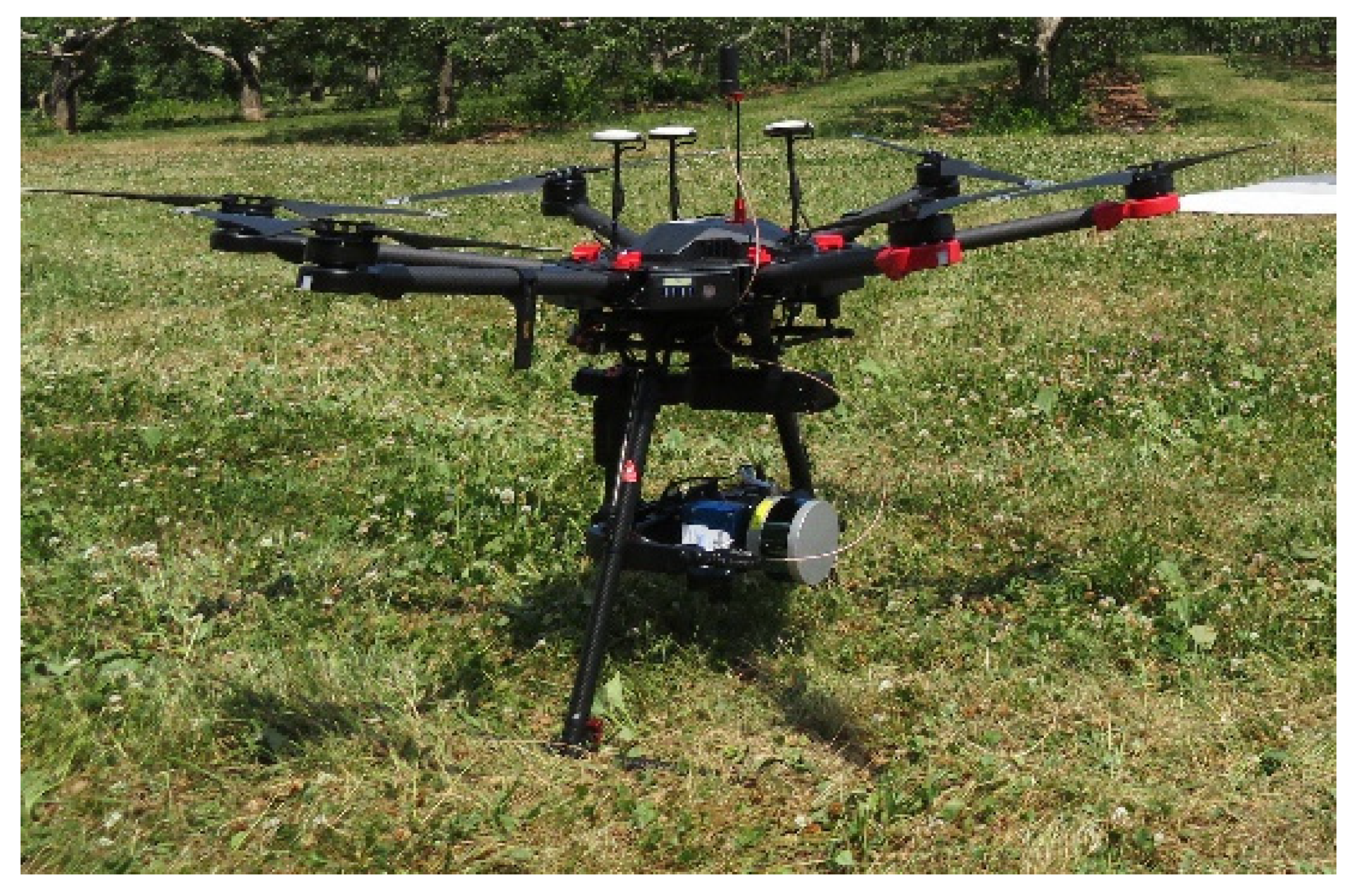
2.3. Creation of the UAS-LiDAR Dataset

A DJI Matrice 600 Pro UAS equipped with a Velodyne VLP-16 LiDAR sensor and an Applanix APX-15 UAS IMU (Table 1, Figure 3) was used to create the UAS-LiDAR dataset, henceforth referred to as LiDAR. The assembled system weighed approximately 11 kg, had a diameter of 170 cm, a maximum speed of 65 km/h, and a flight time of approximately 16 min. Six batteries are required to propel this unit. The LiDAR flight was flown on 20 July 2018 prior to the UAS flights described in Section 2.4. For our mission, the LiDAR was flown at a speed of 10 m/s from 70 m elevation (above ground level) with 50 m strip spacing and 150,000 pulses/second at 180° field of view. The systems captured two returns—the strongest and the last. Post-flight IMU trajectory data were processed using POSPac UAV [44]. GPS base station log files were downloaded from the NSACS station number NS250002 [43]. Data from the IMU and the base station were blended to calculate the aircraft trajectory, stored in Smoothed Best Estimate of Trajectory (SBET) files. Laser returns were downloaded from the LiDAR sensor and processed with the IMU trajectory file in Phoenix Spatial Explorer [45] to create a point cloud dataset. The LiDAR Data Exchange Format (LAS) point cloud data were cleaned using the Statistical Outlier Removal tool in CloudCompare [46] and systematic point data representing point reflections from the legs of the UAS were removed. LiDAR data were analyzed against the survey-grade GPS measurements of elevation from GCPs (Section 2.2) to obtain accuracy values. After verifying the LiDAR data against the 12 checkpoints, the LiDAR had a vertical Root Mean Square Error (RMSE) of ±0.04 m, a mean error (ME) of ±0.03 m, and standard deviation (St. Dev.) of ±0.02 m (Table 2). According to standards developed by the Federal Geographic Data Committee [47] and reported by Evans et al. [48], ±0.04 m is an acceptable vertical error value for LiDAR used in terrain and land cover mapping and was deemed suitable for comparison of UAS DSMs in this study. The LAS file was converted to a raster in ArcGIS Pro 2.1 [49] to create the LiDAR DSM using the LAS Dataset to Raster tool. Before conversion, the LiDAR point cloud density was 343 pts/m2. The triangulation interpolation method was used, and the maximum point value was assigned to each cell in the output raster, representing the top surface of the terrain to creating the DSM. The void fill method was set to linear. Output cell size was 0.10 m and was selected as it provided sufficient detail to distinguish between land cover types and give an accurate representation of the terrain without slowing down processing times.

2.4. UAS Imagery—Data Collection

The four UAS used in this study were Dà-Jiāng Innovations (DJI) Inspire 1 V1 (INS), DJI Matrice 210 (MAT), DJI Mavic Pro (MAV), and the DJI Phantom 4 Professional (P4P). Each was flown three times in random sequence over the study area and each carried a different high-resolution RGB sensor (Table 3). A full battery was used for each flight. Flights were planned with the Pix4D Capture application using a grid pattern (Figure 2c); identical plans were used for each flight. All flights were flown at an altitude of 70 m with 70% front and side overlap and the camera angle at nadir. While 70% is the minimum recommended front overlap for photogrammetric surveys, this value ensured that we would be able to cover the entire study area on one battery for each platform. Respective Ground Sampling Distances (GSDs) are listed in Table 2. Data were collected on July 20, 2018 over a span of approximately 3.5 h from 10:00 to 13:30 AST to avoid shadows. The weather conditions were consistent for the duration of the day, sun with no cloud cover and no wind.

2.5. UAS Imagery—Data Processing Workflow

Aerial images from each UAS flight were processed in the photogrammetric image processing software Agisoft Metashape (Version 1.2.6 Build 2934) [16] according to the USGS-recommended workflow [50]. Each dataset was aligned using a high-accuracy alignment (full image resolution) with system defaults for key point and tie-point limits (50,000; 10,000). Then, the nine Aeropoint GCP targets were manually identified in photos and assigned survey-grade geographic coordinates. Dense point clouds were created at the high-quality setting and were exported in LAS format. Respective point cloud densities are listed in Table 3. Each LAS dataset was converted to a DSM with the LAS to Raster tool in ArcGIS Pro, using triangulation as the interpolation technique, with the points of maximum elevation. Each output DSM was produced with a resolution of 0.10 m to remain consistent with the output LiDAR DSM and to obtain sufficient detail for distinguishing between land cover types while accurately representing the elevation changes across the site and keeping processing times manageable. Orthophoto mosaics were also created from each dense point cloud. Land covers across the study area were manually delineated from an orthophoto mosaic produced from the INS UAS. Land cover was differentiated into six different land cover categories: vines, bare soil, dirt road, mowed grass, long grass and forest.

2.6. Creation of DSMs of Difference (DoDs)

DSMs of Difference (DoDs) were used to compare the DSMs from the UAS against those from LiDAR and visualize spatial differences across the study area. To create DoDs, the LiDAR DSM was subtracted from each UAS DSM in ArcGIS Pro [49]. This created a difference raster for each dataset, where each pixel represented the vertical difference between the aerial image-derived DSM (from UAS) and the LiDAR DSM. These DoD rasters were used to generate four different standard accuracy statistics: ME, St. Dev., Mean Average Error (MAE) and RMSE. ME represents an average of all errors across the DoDs while the St. Dev. measures the error variability. RMSE and MAE scores are interpreted in measured units and do not account for direction of error. However, RMSE is more sensitive to larger errors and increases when variance in error is high. MAE is easier to interpret, showing the average, absolute difference between predicted and measured values. DoDs enabled the visualization of spatial differences between the two data collection methods across the study area [51].

3. Results

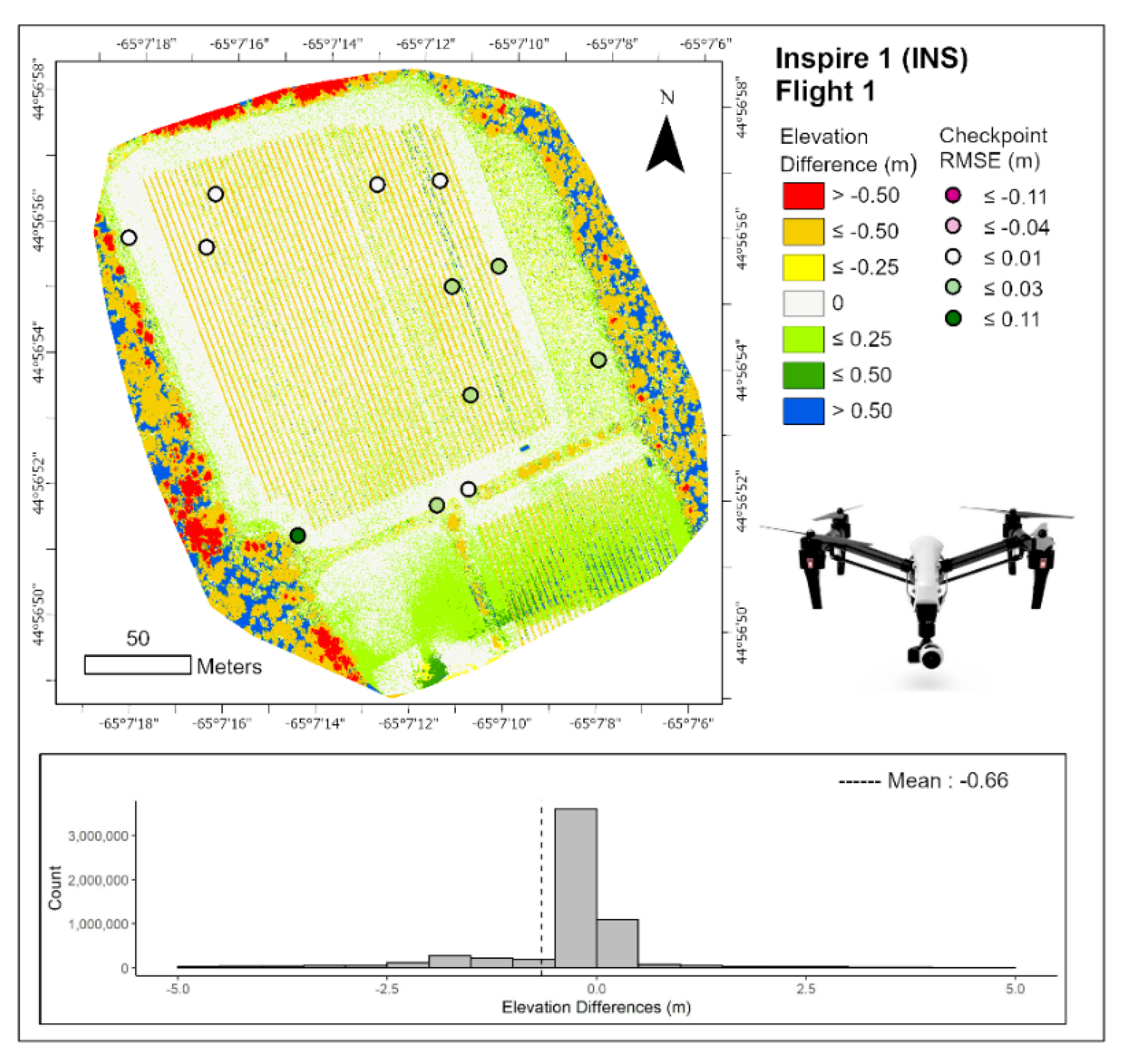
3.1. Accuracy of UAS DSMs Compared to Checkpoints and DSMs of Difference (DoDs)

The details of each UAS flight including start time, order, duration, number of images, resulting point cloud density, and statistics of output DSMs compared to 12 checkpoints are listed in Table 4. Based on these results, the best flight was chosen for each platform (shown in bold) and elaborated in the sections below. We determined the best flights to be those with the lowest error values overall. Locations of checkpoints are shown in Figure 2 and associated error values for each checkpoint are listed in Supplementary Table S1 (Table S1). DoDs were created by subtracting the LiDAR DSM from each UAS DSM to determine where spatial differences occurred across the study area. These statistics are listed in Table 5 and shown in Figure 4, Figure 5, Figure 6 and Figure 7.

3.1.1. DJI Inspire 1 (INS)

INS is the second heaviest (3060 g), has the shortest flight time (18 min), the second lowest sensor resolution (12.4 MP), and a 1/2.3″ CMOS sensor (Table 3). It is the oldest of the studied platforms (2014), and the second most expensive at the time of purchase. For this platform, each flight was of similar duration with identical number of images collected (117) (Table 4). INS had the coarsest GSD (3.06 cm/px) and lowest output point cloud density overall (434.03 pts/m2).
Compared to the 12 checkpoints, the most accurate flight was flight number one (Table 4). RMSE values ranged from −0.03 m to 0.08 m across the site (Figure 4, circles; Table S1). Overall, INS had the second highest ME (0.01 m) and tied for lowest St. Dev. (0.03 m), MAE (0.02 m), and RMSE (0.03 m).
Compared to the LiDAR DSM, the INS DoD had the second lowest ME (−0.66 m), St. Dev. (2.37 m), and MAE (0.95 m) (Table 5). The overall RMSE for this flight was highest at 2.09 m. The high St. Dev. value indicates that there are inconsistencies in error across the study site while the negative mean error value indicates that the INS DSM consistently underestimates elevation. As seen in the spatial errors across the DoD for the INS platform (Figure 4), the lowest error values are seen on non-vegetated terrain, while the highest errors are in areas covered by vegetation—in this case, forest and vines.

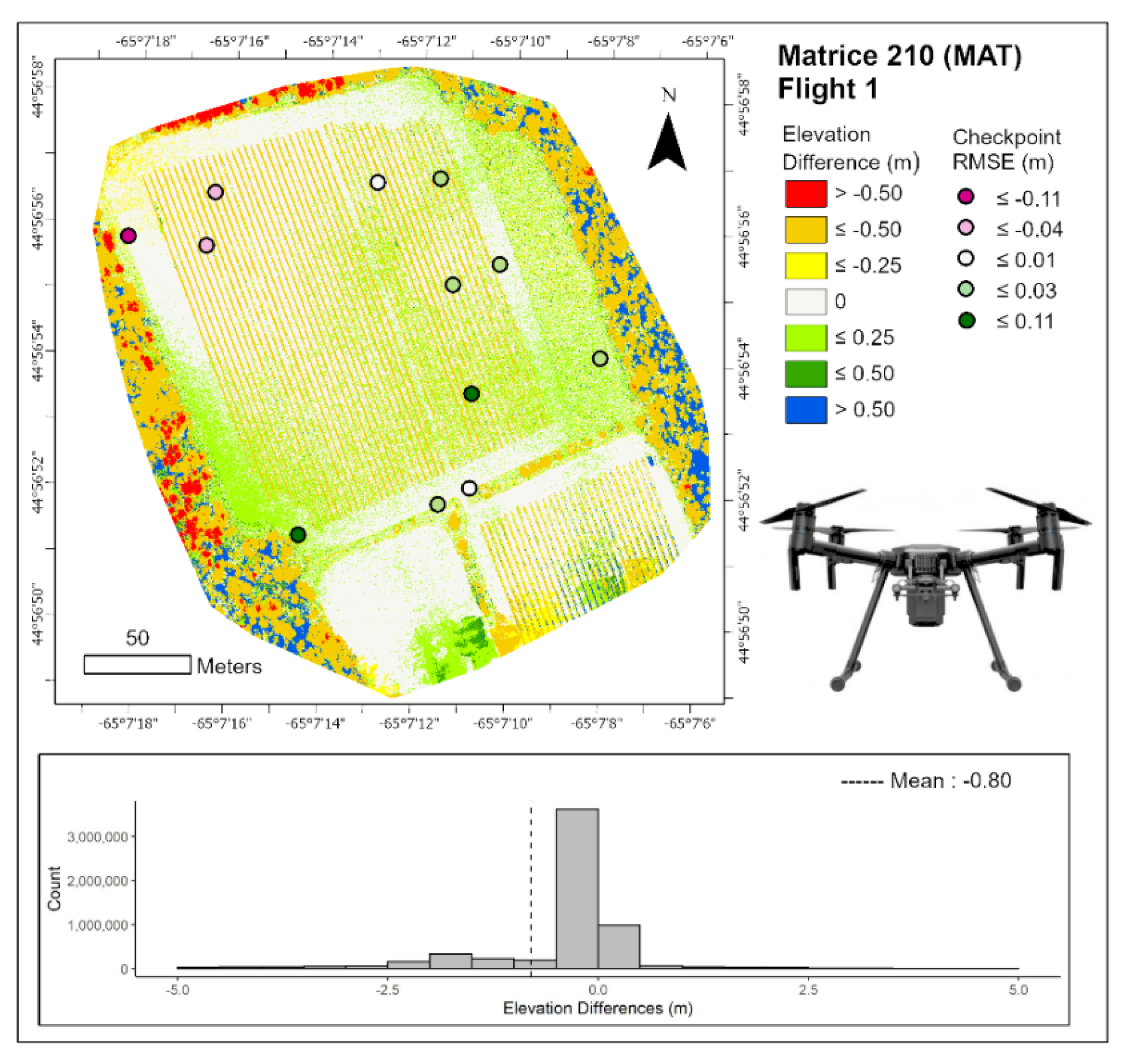
3.1.2. DJI Matrice 210 (MAT)

MAT is the heaviest (4570 g), has the longest flight time (38 min), the highest sensor resolution (20.8 MP), and a 4/3″ CMOS sensor (Table 3). It is one of the newest of the studied platforms (2017) and the most expensive. For this platform, flight one was longer than flight two and three by approximately one and a half minutes, and thus collected 216 images rather than the 160 images for the other flights. This resulted from a lost connection between the UAS and the remote controller due to overheating of the tablet and an extra flight line was flown. MAT had the finest GSD (1.55 cm/px) and output point cloud densities overall (1371.70 pts/m2).
Compared to the 12 checkpoints, the most accurate flight was flight number one (Table 4). RMSE values ranged from −0.15 m to 0.11 m across the site (Figure 5, circles; Table S1), which was the largest range among platforms. Overall, MAT had the lowest ME (0.003 m), highest St. Dev. (0.07 m) and tied for highest MAE (0.05 m) and RMSE (0.06 m).
Compared to the LiDAR DSM (Table 5), the MAT DoD had the highest ME (−0.80 m), second highest St.Dev. (2.43 m) and MAE (1.02 m), and lowest overall RMSE (1.97 m). The negative mean error values indicate that the MAT DSM consistently underestimates elevation values. As seen in the DoD for the MAT platform (Figure 5), the lowest error values can be seen on non-vegetated terrain, while the highest errors are in vegetated terrain.

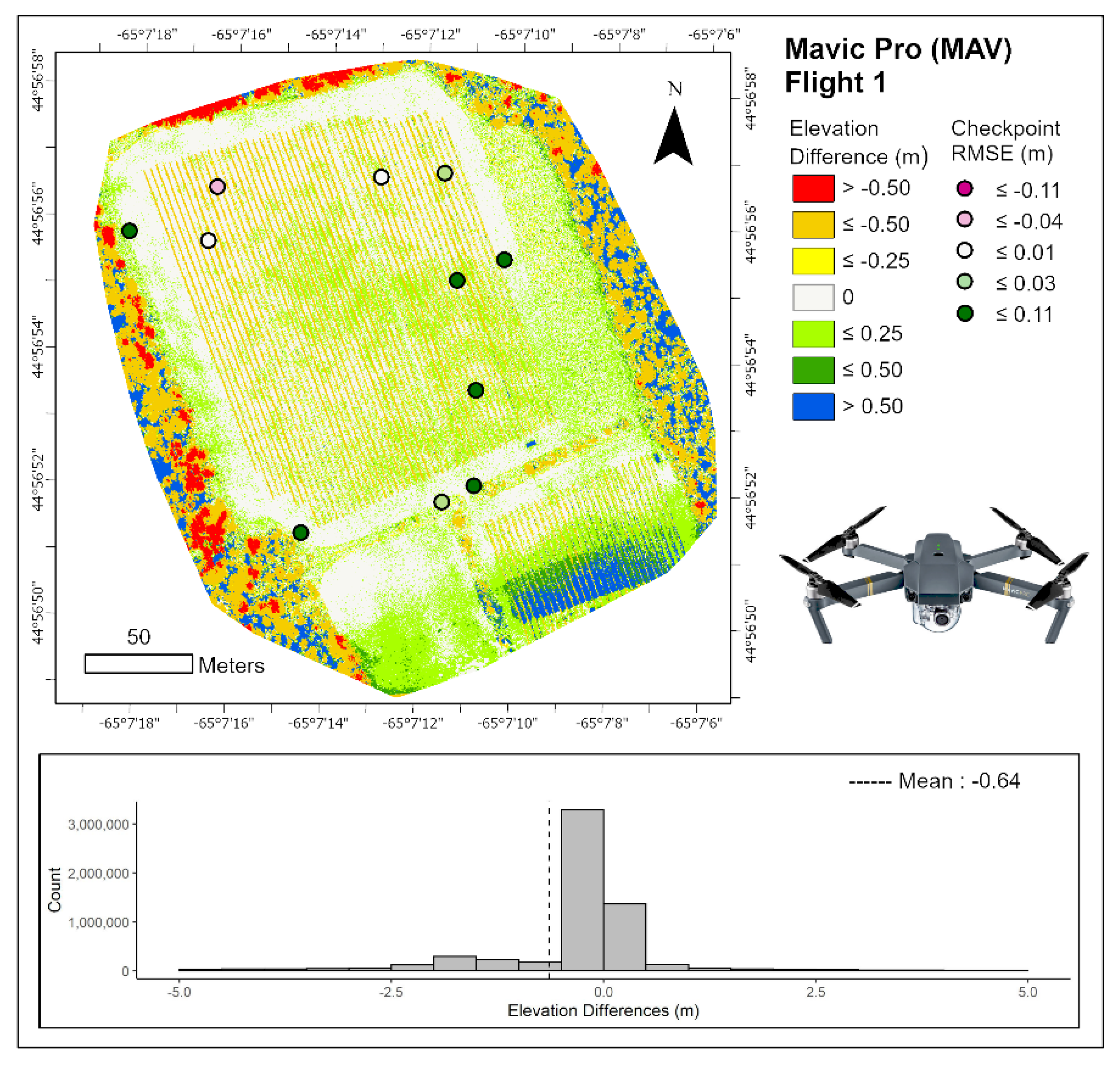
3.1.3. DJI Mavic Pro (MAV)

The MAV is the smallest and lightest (734 g) of all UAS used in this study. It has the lowest resolution sensor (12.35 MP), a CMOS sensor of 1/2.3″, second shortest flight time, and is the least expensive (Table 3). Flights times differed by 30 s for each flight but acquired similar numbers of images (177, 176, and 176 respectively). This platform had the second finest GSD (2.3 cm/px) and output point cloud densities overall (730.60 pts/m2).
Compared to the 12 checkpoints (Table 4), the most accurate flight was flight number one. RMSE values ranged from −0.06 m to 0.08 m across the site (Figure 6, circles; Table S1). MAV had the worst overall accuracy values when compared to the other platforms, highest ME (0.04 m), second highest St. Dev. (0.05 m), and tied for highest MAE (0.05 m) and RMSE (0.06 m).
Compared to the LiDAR DSM, the MAV DoD had the lowest mean error (−0.64 m), St. Dev. (2.33 m), and MAE (0.94 m) (Table 5). MAV had the second lowest overall RMSE (2.03) m. The negative mean error values indicate that the MAV DSMs consistently underestimate elevation values. As seen in the DoD for the MAV platform (Figure 6), the lowest error values can be seen on non-vegetated terrain, while the highest errors are in vegetated terrain.

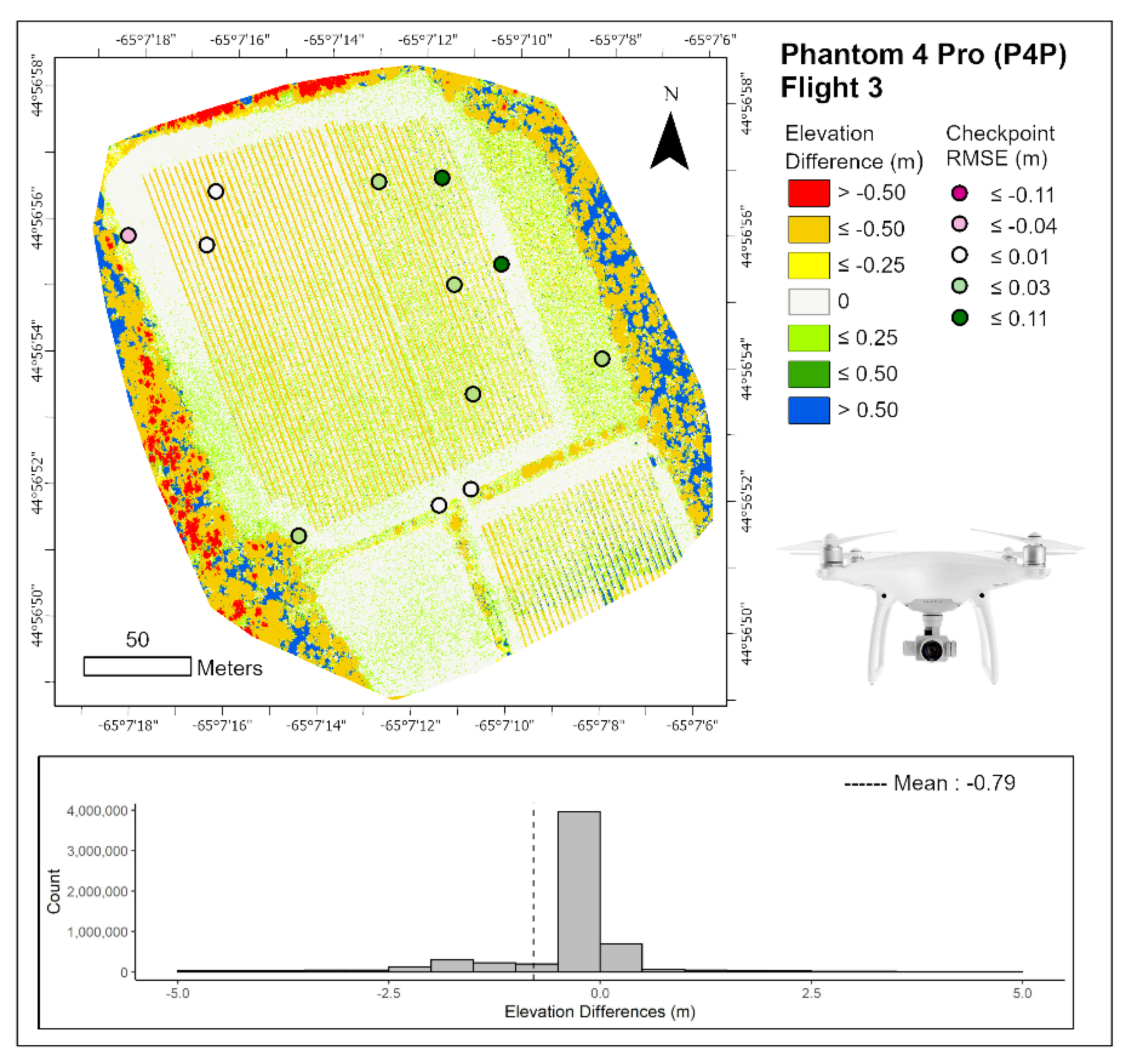
3.1.4. Phantom 4 Professional (P4P)

The P4P is the second lightest (1388 g), has the second longest flight time (30 min), the second highest sensor resolution (20 MP), and a 1″ CMOS (Table 1). It is the second oldest studied platforms (2016) and the third most expensive. The flight durations varied between 8 min 10 s and 10 min 36 s. Flight one was over two minutes shorter than flights two and three, thus acquired fewer images (146 versus 160) due to extra flights lines automatically added by the Pix4D app. This platform had the second coarsest GSD (1.91 cm/px) and output point cloud densities overall (1040.58 pts/m2).
Compared to the 12 checkpoints (Table 4), the most accurate flight was flight number three. RMSE values ranged from −0.05 m to 0.03 m across the site (Figure 6, circles; Table S1), the smallest range in values among platforms. P4P had the second highest ME (0.007 m), and tied to lowest St. Dev. (0.03 m), MAE (0.02 m) and RMSE (0.03 m) when compared to the other platforms.
Compared to the LiDAR DSM, the P4P DoD had the second highest mean error (−0.79 m); highest St. Dev. (2.58 m) and MAE (1.03 m) (Table 5). P4P had the second highest overall RMSE (2.04 m). The negative mean error values indicate that the P4P DSM consistently underestimates elevation values. As seen in the DoD for the P4P platform (Figure 7), the lowest error values can be seen on non-vegetated terrain, while the highest errors are in vegetated areas.

3.2. Differences across Land Covers

DoDs were re-examined by their respective land cover categories and statistics (ME, St. Dev., MAE, and RSME) (Table 6) were generated to quantify errors due to differing land covers. Collectively, the UAS performed best in the categories of (in descending order) dirt road, mowed grass, bare soil, vines, long grass, and forest. ME values were predominantly negative (except for INS and MAV in the dirt road category), indicating that the UAS DSMs were consistently lower in elevation than the LiDAR DSM. ME values in the bare soil, dirt road, and mowed grass categories were comparable to the overall LiDAR DSM ME value of 0.03 m.

3.3. Summary of UAS Performance

The performance of each UAS was ranked according to several of its physical parameters (i.e., dimensions, weight, flight time, number of batteries required, and resulting GSD based on sensor resolution) and quantitative statistics calculated throughout this study (Table 7). For example, MAV is the smallest and lightest, thus was ranked best (1) in those categories. MAT has the longest flight time, although it required two batteries for operation. All other platforms required one battery and were tied for best (1) in this category, while MAT took second place (2). The GSD was a direct reflection of the sensor resolution on each device and was ranked from best to worst (MAT [1], P4P [2], MAV [3], and INS [4]) and assigned values, respectively. P4P and MAV were tied for first with nine points overall in the physical parameters group, with MAT second and INS third.
In the statistics group, platforms were ranked on their respective RMSE values compared to checkpoints, DoD, and each land cover category. Compared to checkpoints, INS and P4P tied for first, while MAT and MAV tied for second. Compared to overall DoDs calculated by subtracting the LiDAR DSM from respective UAS DSMs, the order of ranking from best to worst was MAT, MAV, P4P, and INS. Each platform was also ranked based on RMSE values over each land cover category, with P4P performing best overall; first place in four of six categories (vines, bare soil, forest and mowed grass), and MAV worst overall; last place in three of six categories (vines, bare soil, and forest). In summary, P4P was the clear front runner overall, with the lowest total points (21). The second, third, and fourth place rankings were relatively close with MAV (31 points), MAT (33 points) and INS (34 points), respectively.

4. Discussion

4.1. LiDAR Data Collection, Processing and Accuracy

The LiDAR data collected in this study showed promising results for the construction of DSMs for local-scale surveys. LiDAR gave an accurate representation of the terrain (ME: 0.03 m, St. Dev.: 0.02 m, MAE: 0.04 m, and RMSE: 0.04 m) and was effectively used to compare the test UAS. The LiDAR DSM was clearly superior to the UAS DSMs over vegetated terrain. This was expected due to the inherent nature of the employed devices [19] and is further supported in the literature [34]. Compared to airborne and terrestrial LiDAR campaigns, UAS LiDAR gives the researcher more flexibility in determining when and where the data are collected. However, the limited battery life highly limits the size of the study area. Moreover, the collection of LiDAR data from a UAS is problematic in terms of calibration of the IMU, system set up, and processing. As UAS LiDAR is still relatively new, the development of a working field methodology took three weeks to establish a process that worked for our needs. We utilized a process where we flew the UAS forward at full speed for 10 s, brought it to a rapid stop, then flew it back at full speed for another rapid stop. This movement helped calibrate the IMU by giving it spikes in the accelerometer data, as IMUs perform best when they experience rapid movement. We found that the relatively slow movements of a UAS flight can cause the IMU to drift and these rapid movements before data collection helped give the IMU inertial reference information to help calibrate the rest of the flight. This shows the importance of integration of IMU and GNSS receivers on any airborne LiDAR system (c.f. [52]). Other researchers discussed similar difficulties when collecting LiDAR data [53]. As the technology continues to develop, the weight of the platform and expense of batteries will decrease, and the flight time will increase. In fact, since the time of purchase in 2017, the cost of a Velodyne VLP-16 LiDAR has dropped by more than 50% due to the tremendous demand for the product, predominantly related to development of the autonomous vehicle industry [54]. Although UAS camera sensors in conjunction with advanced photogrammetric processing techniques have advanced enormously in recent years, their ability to produce accurate DSMs and orthomosaics in vegetated environments is still lacking compared to LiDAR. LiDAR remains to be the best option for obtaining high accuracy data in complex terrain and vegetated environments. UAS LiDAR is an efficient option for local scales; yet the specific application will determine the need for the investment into a UAS LiDAR.

4.2. Overall Accuracy of UAS DSMs Compared to Checkpoints and DSMs

Results show that the overall accuracy of UAS DSMs compared to checkpoints was high (Table 4). However, the locations of these checkpoints were on non-vegetated terrain and at ground level (Figure 2a) and thus do not reflect with certainty the accuracy of UAS DSMs at canopy height nor in vegetated areas, specifically. To do this sufficiently, checkpoints should be located on top of trees and/or among the trees, which was not possible at the time of data collection. Yet, RMSE values across platforms ranged from ±0.03 m (INS and P4P) to ±0.06 m (MAT and MAV) compared to the LiDAR DSM, which had an overall RMSE of ±0.04 m. Both the MAT and P4P had very low ME values (0.003 m and 0.007 m, respectively) indicating overall subcentimeter vertical accuracy compared to checkpoints. These platforms had the highest-resolution camera sensors (MAT: 20.8 MP and P4P: 20 MP), and therefore the GSDs (MAT: 1.55 cm/px and P4P: 1.91 cm/px) and output point cloud densities (MAT: 1371.70 pts/m2 and P4P: 1040.58 pts/m2) were also higher than the other two platforms. Although the ME values were lower for the MAT and the P4P, the overall RMSEs were comparable to the INS and MAV platforms which had lower sensor resolution (INS: 12.4 MP and MAV: 12.35 MP), GSDs (INS: 3.06 cm/px and MAV: 2.3 cm/px) and output point cloud densities (INS: 434.03 pts/m2 and MAV: 730.60 pts/m2) overall. This indicates that when using an output resolution of 0.10 m for the DSM, the interpolation obscured the fine-scale differences resulting from different sensor resolutions. Each of the UAS performed well at the 0.10 m DSM output resolution. For broad-scale mapping applications (e.g., terrain mapping, precision agriculture, land cover classification) the 0.10 m resolution was sufficient. However, this may not hold true for finer DSM resolutions. For example, with output DSMs at 0.01 m, the differences across platforms may become more evident and should be investigated in the future.
DoDs were calculated to compare each UAS DSM to the LiDAR DSM to visualize spatial differences across the study area. This process showed distinct patterns of high agreement in non-vegetated areas and high disagreement over vegetation terrain. This stems from (1) the differences between how the measurements were taken, photogrammetry versus LiDAR, with LiDAR being inherently superior in vegetated terrain; (2) on the locations of the GCPs used to rectify UAS point clouds during the photogrammetric process which were located on non-vegetated terrain and at ground elevation (Figure 2a). Thus, vegetated areas and tree canopies were not sufficiently referenced by the GCPs. The large elevation differences between the UAS DSMs and the LiDAR DSMs, especially in forested areas, may stem from the lack of validation of the vertical distribution of heights across the study site. Additionally, there was higher uncertainty in output UAS DSMs outside of the GCP coverage areas, which coincided to forested areas and the southern portion of the site. These errors were further propagated in the creation of each DoD, which is evident in the very high difference values (>0.50 m and <0.50 m) on the borders of the DoDs in Figure 4, Figure 5, Figure 6 and Figure 7. Thus, further discussion will focus on non-vegetated areas.
The DoDs provide an indicator for measuring how each UAS performed compared to the LiDAR over the entire study site. RMSE values were calculated for the UAS (ranging from ±1.97 m [MAT] to ±2.09 m [INS]) (Table 5). When re-examined by land cover category, UAS DSMs showed highest discrepancies compared to the LiDAR DSM over vegetated terrain and collectively performed best over non-vegetated terrains. In terms of relative performance among the UAS, the P4P performed best, with lowest RMSE values in four of six categories (vines, bare soil, forest, and mowed grass), while the MAT performed worst overall, with highest RMSE values in three of six categories (vines, bare soil, and forest). However, all platforms performed comparably to LiDAR over non-vegetated terrains. When considering ME metrics, MAV performed best in five of six land cover categories (all except forest). This is interesting, since the MAV platform is smallest and lightest, has the lowest resolution sensor, and is the least expensive. In general, P4P had higher accuracy outside of the GCPs (Figure 7). This is visible in the southern part of the study area. The noise displayed in in the southern parts of other platforms’ DoDs is likely a result of those locations being on the edges of the study area where there are fewer overlapping images and not covered by GCPs, thus fewer images available for matching and dense point cloud construction.
Overall, all the UAS were comparable in their accuracy to checkpoints and DoDs showed that each consistently underestimated elevation compared to the LiDAR DSM. The specifications of each platform varied most widely among the resolution of the RGB sensor, with the INS and MAT having the lowest resolutions (12.35 and 12.4 MP, respectively), and the P4P and MAT having the highest-resolution sensors (20 and 20.8 MP, respectively). Higher sensor resolutions are tied directly to finer GSDs and greater density in output point clouds. In the end, with the 0.10 m resolution used for the output DSMs, all platforms performed comparably to each other. To summarize all findings across the study, a summary schema was used to calculate overall rankings (Section 3.3; Table 7). These rankings clearly indicated that P4P was the front runner of all systems (21 points overall). This can be attributed to its unique balance between manageable size and high sensor resolution; thus it is ranked in first place. This ranking scheme gives preference to smaller platforms due purely to manageability in transport and flight. However, there are benefits to larger platforms as well. Larger platforms (i.e., P4P, MAT and INS) have the ability to carry additional sensors that can be attached to the frame to collect other remote sensing data (e.g., thermal or multispectral), while the MAV is too small to attach other external sensors. Both the MAT and INS have the functionality to change the attached sensors, while the P4P and MAV do not. However, within this ranking, MAV came in second place, with 31 points and was the smallest of studied platforms. MAT came in third place, with 33 points, and INS in fourth place, with 34 points. The second, third, and fourth place overall results are numerically close and thus it would be difficult to choose a clear front runner from the remaining three platforms. Instead, the application and environmental setting necessitating data collection will ultimately dictate which platform to use. Although, results indicate that the P4P is the best product for the cost, and perhaps the best-rounded of platforms. While this ranking schema is not perfect, it does allow each platform to be judged objectively using a number of metrics.

5. Conclusions

The results of this study reiterate how LiDAR is best for vegetation mapping and provide further evidence for the usefulness of LiDAR on a UAS. While the costs of UAS-LiDAR continue to decrease, including both the monetary and time investments, they are still more expensive than off-the-shelf UAS. Seeing that UAS DSMs were comparable to the LiDAR DSM at the 0.10 m scale over most land covers in this study (except over vegetated terrain), the application for which data are being collected will ultimately determine which platform is needed. Additionally, more testing is needed to determine whether UAS DSMs at finer resolution perform similarly compared to LiDAR. Among the UAS themselves, the P4P was the clear front runner due to its balance between size and sensor resolution. The specific application and required functionality will determine which UAS to use in future studies, but the P4P seems to be the most well rounded and best value for the cost of the tested platforms.

Supplementary Materials

The following are available online at https://www.mdpi.com/2072-4292/12/17/2806/s1, Table S1: Locations of checkpoints (CP) in decimal degrees, altitude (m) of each checkpoint, and differences between respective DSMs and checkpoints in meters (m) listed by platform: LiDAR, INS (Inspire), MAT (Matrice), MAV (Mavic Pro), P4P (Phantom 4 Pro). Overall Mean Error (ME), Standard Deviation of Error (St. Dev.), Mean Average Error (MAE), and RMSE also listed.

Author Contributions

Conceptualization, S.R.R. and W.L.; Methodology, S.R.R., W.L., and I.M.; Validation, S.R.R., W.L., and I.M.; Formal Analysis, S.R.R. and I.M.; Resources, S.R.R. and W.L.; Writing—Original Draft Preparation, S.R.R. and I.M.; Writing—Review and Editing, S.R.R., W.L., and I.M.; Visualization, S.R.R. and I.M. All authors have read and agreed to the published version of the manuscript.

Funding

This research received no external funding.

Acknowledgments

The authors would like to thank Paul Illsley for his support in fieldwork preparations and data acquisition.

Conflicts of Interest

The authors declare no conflict of interest.

References

  1. Campbell, J.; Shin, M. Essentials of Geographic Information Systems; Saylor: Washington, DC, USA, 2011; ISBN 978-1-4533-2196-6. [Google Scholar]
  2. Ritchie, J.C. Airborne laser altimeter measurements of landscape topography. Remote Sens. Environ. 1995, 53, 91–96. [Google Scholar] [CrossRef]
  3. Taud, H.; Parrot, J.-F.; Alvarez, R. DEM generation by contour line dilation. Comput. Geosci. 1999, 25, 775–783. [Google Scholar] [CrossRef]
  4. Chasmer, L.; Hopkinson, C.; Treitz, P. Investigating laser pulse penetration through a conifer canopy by integrating airborne and terrestrial lidar. Can. J. Remote Sens. 2006, 32, 116–125. [Google Scholar] [CrossRef] [Green Version]
  5. Open Topography. Available online: https://opentopography.org/ (accessed on 17 June 2020).
  6. NOAA. Data Access Viewer. Available online: https://coast.noaa.gov/dataviewer/#/lidar/search/ (accessed on 17 June 2020).
  7. USGS. LidarExplorer. Available online: https://prd-tnm.s3.amazonaws.com/LidarExplorer/index.html#/ (accessed on 17 June 2020).
  8. Nex, F.; Remondino, F. UAV for 3D mapping applications: A review. Appl. Geomat. 2014, 6, 1–15. [Google Scholar] [CrossRef]
  9. Colomina, I.; Molina, P. Unmanned aerial systems for photogrammetry and remote sensing: A review. ISPRS J. Photogramm. Remote Sens. 2014, 92, 79–97. [Google Scholar] [CrossRef] [Green Version]
  10. Honkavaara, E.; Saari, H.; Kaivosoja, J.; Pölönen, I.; Hakala, T.; Litkey, P.; Mäkynen, J.; Pesonen, L. Processing and assessment of spectrometric, stereoscopic imagery collected using a lightweight UAV spectral camera for precision agriculture. Remote Sens. 2013, 5, 5006–5039. [Google Scholar] [CrossRef] [Green Version]
  11. Haala, N.; Brenner, C. Extraction of buildings and trees in urban environments. ISPRS J. Photogramm. Remote Sens. 1999, 54, 130–137. [Google Scholar] [CrossRef]
  12. Priestnall, G.; Jaafar, J.; Duncan, A. Extracting urban features from LiDAR digital surface models. Comput. Environ. Urban Syst. 2000, 24, 65–78. [Google Scholar] [CrossRef]
  13. Torresan, C.; Berton, A.; Carotenuto, F.; Gennaro, S.F.D.; Gioli, B.; Matese, A.; Miglietta, F.; Vagnoli, C.; Zaldei, A.; Wallace, L. Forestry applications of UAVs in Europe: A review. Int. J. Remote Sens. 2017, 38, 2427–2447. [Google Scholar] [CrossRef]
  14. Frueh, C.; Zakhor, A. Constructing 3D city models by merging ground-based and airborne views. In Proceedings of the IEEE Computer Society Conference on Computer Vision and Pattern Recognition, Madison, WI, USA, 18–20 June 2003. [Google Scholar] [CrossRef] [Green Version]
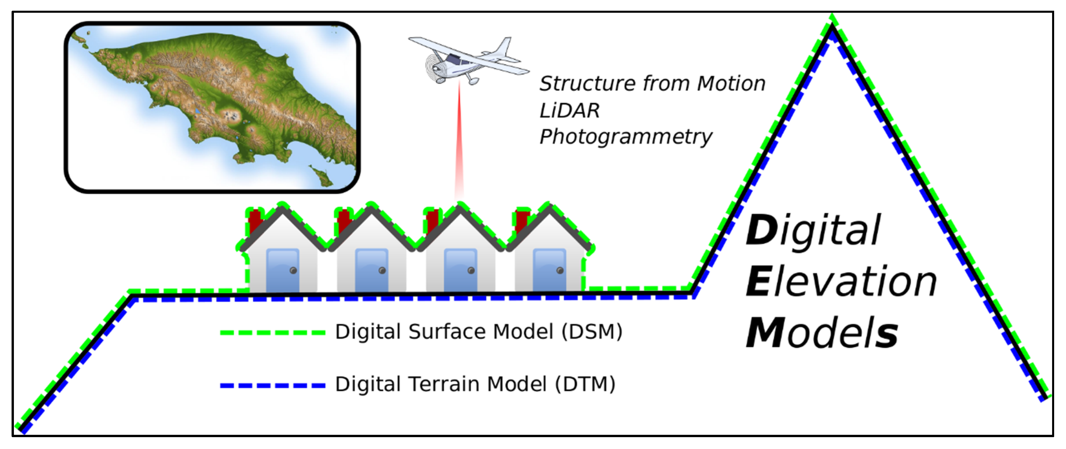
  15. Arbeck. The Difference between Digital Surface Model (DSM) and Digital Terrain Models (DTM) when Talking about Digital Elevation Models (DEM). 2015. Available online: https://commons.wikimedia.org/wiki/File:The_difference_between_Digital_Surface_Model_(DSM)_and_Digital_Terrain_Models_(DTM)_when_talking_about_Digital_Elevation_models_(DEM).svg (accessed on 23 August 2020).
  16. Agisoft Metashape. Available online: https://www.agisoft.com/ (accessed on 17 June 2020).
  17. Pix4D. Pix4Dmapper: Professional Drone Mapping and Photogrammetry Software. Available online: https://www.pix4d.com/product/pix4dmapper-photogrammetry-software (accessed on 17 June 2020).
  18. Hashemi-Beni, L.; Jones, J.; Thompson, G.; Johnson, C.; Gebrehiwot, A. Challenges and opportunities for UAV-based digital elevation model generation for flood-risk management: A case of Princeville, North Carolina. Sensors 2018, 18, 3843. [Google Scholar] [CrossRef] [Green Version]
  19. Mandlburger, G.; Wenzel, K.; Spitzer, A.; Haala, N.; Glira, P.; Pfeifer, N. Improved topographic models via concurrent airborne LiDAR and dense image matching. ISPRS Ann. Photogramm. Remote Sens. Spat. Inf. Sci. 2017, 4, 259–266. [Google Scholar] [CrossRef] [Green Version]
  20. Jensen, J.L.R.; Mathews, A.J. Assessment of image-based point cloud products to generate a bare Earth surface and estimate canopy heights in a woodland ecosystem. Remote Sens. 2016, 8, 50. [Google Scholar] [CrossRef] [Green Version]
  21. Salach, A.; Bakuła, K.; Pilarska, M.; Ostrowski, W.; Górski, K.; Kurczyński, Z. Accuracy assessment of point clouds from LiDAR and dense image matching acquired using the UAV platform for DTM creation. ISPRS Int. J. Geo-Inf. 2018, 7, 342. [Google Scholar] [CrossRef] [Green Version]
  22. Schonberger, J.L.; Frahm, J.-M. Structure-from-motion revisited. In Proceedings of the IEEE Conference on Computer Vision and Pattern Recognition (CVPR), Las Vegas, NV, USA, 27–30 June 2016; pp. 4104–4113. [Google Scholar] [CrossRef]
  23. Fonstad, M.A.; Dietrich, J.T.; Courville, B.C.; Jensen, J.L.; Carbonneau, P.E. Topographic structure from motion: A new development in photogrammetric measurement. Earth Surf. Process. Landf. 2013, 38, 421–430. [Google Scholar] [CrossRef] [Green Version]
  24. Pricope, N.G.; Mapes, K.L.; Woodward, K.D.; Olsen, S.F.; Baxley, J.B. Multi-sensor assessment of the effects of varying processing parameters on UAS product accuracy and quality. Drones 2019, 3, 63. [Google Scholar] [CrossRef] [Green Version]
  25. Hirschmuller, H. Stereo processing by semiglobal matching and mutual information. IEEE Trans. Pattern Anal. Mach. Intell. 2008, 30, 328–341. [Google Scholar] [CrossRef] [PubMed]
  26. Rothermel, M.; Wenzel, K.; Fritsch, D.; Haala, N. SURE: Photogrammetric surface reconstruction from imagery. In Proceedings of the LC3D Workshop, Berlin, Germany, 4–5 December 2012; Volume 8. [Google Scholar]
  27. Wenzel, K.; Rothermel, M.; Haala, N.; Fritsch, D. SURE–The ifp software for dense image matching. In Proceedings of the Photogrammetric Week, Stuttgart, Germany, 9–13 September 2013; Volume 13, pp. 59–70. [Google Scholar]
  28. Remondino, F.; Spera, M.G.; Nocerino, E.; Menna, F.; Nex, F.; Gonizzi-Barsanti, S. Dense image matching: Comparisons and analyses. In Proceedings of the Digital Heritage International Congress, Marseille, France, 28 October–1 November 2013; Volume 1, pp. 47–54. [Google Scholar]
  29. Gašparović, M.; Seletković, A.; Berta, A.; Balenović, I. The evaluation of photogrammetry-based DSM from low-cost UAV by LiDAR-based DSM. South-East Eur. For. 2017, 8. [Google Scholar] [CrossRef] [Green Version]
  30. Gauci, A.A.; Brodbeck, C.J.; Poncet, A.M.; Knappenberger, T. Assessing the geospatial accuracy of aerial imagery collected with various UAS platforms. Trans. ASABE 2018, 61, 1823–1829. [Google Scholar] [CrossRef]
  31. Coveney, S.; Roberts, K. Lightweight UAV digital elevation models and orthoimagery for environmental applications: Data accuracy evaluation and potential for river flood risk modelling. Int. J. Remote Sens. 2017, 38, 3159–3180. [Google Scholar] [CrossRef] [Green Version]
  32. Agüera-Vega, F.; Carvajal-Ramírez, F.; Martínez-Carricondo, P. Accuracy of digital surface models and orthophotos derived from unmanned aerial vehicle photogrammetry. J. Surv. Eng. 2017, 143, 1–10. [Google Scholar] [CrossRef]
  33. Mancini, F.; Dubbini, M.; Gattelli, M.; Stecchi, F.; Fabbri, S.; Gabbianelli, G. Using unmanned aerial Vehicles (UAV) for high-resolution reconstruction of topography: The structure from motion approach on coastal environments. Remote Sens. 2013, 5, 6880–6898. [Google Scholar] [CrossRef] [Green Version]
  34. Wallace, L.; Lucieer, A.; Malenovský, Z.; Turner, D.; Vopěnka, P. Assessment of forest structure using two UAV techniques: A comparison of airborne laser scanning and structure from motion (SfM) point clouds. Forests 2016, 7, 62. [Google Scholar] [CrossRef] [Green Version]
  35. Yao, H.; Qin, R.; Chen, X. Unmanned aerial vehicle for remote sensing applications—A review. Remote Sens. 2019, 11, 1443. [Google Scholar] [CrossRef] [Green Version]
  36. Sankey, T.T.; McVay, J.; Swetnam, T.L.; McClaran, M.P.; Heilman, P.; Nichols, M. UAV hyperspectral and lidar data and their fusion for arid and semi-arid land vegetation monitoring. Remote Sens. Ecol. Conserv. 2018, 4, 20–33. [Google Scholar] [CrossRef]
  37. Brede, B.; Lau, A.; Bartholomeus, H.M.; Kooistra, L. Comparing RIEGL RiCOPTER UAV LiDAR derived canopy height and DBH with terrestrial LiDAR. Sensors 2017, 17, 2371. [Google Scholar] [CrossRef] [PubMed]
  38. Cao, L.; Liu, K.; Shen, X.; Wu, X.; Liu, H. Estimation of forest structural parameters using UAV-LiDAR data and a process-based model in ginkgo planted forests. IEEE J. Sel. Top. Appl. Earth Obs. Remote Sens. 2019, 1–16. [Google Scholar] [CrossRef]
  39. Khan, S.; Aragão, L.; Iriarte, J. A UAV–lidar system to map Amazonian rainforest and its ancient landscape transformations. Int. J. Remote Sens. 2017, 38, 2313–2330. [Google Scholar] [CrossRef]
  40. Liang, X.; Wang, Y.; Pyörälä, J.; Lehtomäki, M.; Yu, X.; Kaartinen, H.; Kukko, A.; Honkavaara, E.; Issaoui, A.E.I.; Nevalainen, O.; et al. Forest in situ observations using unmanned aerial vehicle as an alternative of terrestrial measurements. For. Ecosyst. 2019, 6, 20. [Google Scholar] [CrossRef] [Green Version]
  41. Sofonia, J.; Shendryk, Y.; Phinn, S.; Roelfsema, C.; Kendoul, F.; Skocaj, D. Monitoring sugarcane growth response to varying nitrogen application rates: A comparison of UAV SLAM LiDAR and photogrammetry. Int. J. Appl. Earth Obs. Geoinf. 2019, 82, 101878. [Google Scholar] [CrossRef]
  42. Giordan, D.; Adams, M.S.; Aicardi, I.; Alicandro, M.; Allasia, P.; Baldo, M.; De Berardinis, P.; Dominici, D.; Godone, D.; Hobbs, P. The use of unmanned aerial vehicles (UAVs) for engineering geology applications. Bull. Eng. Geol. Environ. 2020, 1–45. [Google Scholar] [CrossRef] [Green Version]
  43. Province of Nova Scotia GeoNOVA. Available online: https://geonova.novascotia.ca/ (accessed on 10 March 2020).
  44. Applanix POSPac UAV. Available online: https://www.applanix.com/downloads/products/specs/POSPac-UAV.pdf (accessed on 17 June 2020).
  45. Phoenix LiDAR Systems. Phoenix Spatial Explorer. Available online: https://www.phoenixlidar.com/software/ (accessed on 22 July 2020).
  46. CloudCompare. (Version 2.1). Available online: http://www.cloudcompare.org/ (accessed on 17 June 2020).
  47. Federal Geographic Data Committee Geospatial Positioning Accuracy Standards. Available online: https://www.fgdc.gov/standards/projects/FGDC-standards-projects/accuracy/part1/chapter1 (accessed on 14 May 2020).
  48. Evans, J.S.; Hudak, A.T.; Faux, R.; Smith, A.M.S. Discrete return lidar in natural resources: Recommendations for project planning, data processing, and deliverables. Remote Sens. 2009, 1, 776. [Google Scholar] [CrossRef] [Green Version]
  49. Esri ArcGIS Pro. 2D and 3D GIS Mapping Software. Available online: https://www.esri.com/en-us/arcgis/products/arcgis-pro/overview (accessed on 17 June 2020).
  50. USGS Agisoft Photoscan Workflow. Available online: https://uas.usgs.gov/nupo/pdf/USGSAgisoftPhotoScanWorkflow.pdf (accessed on 14 May 2020).
  51. Lague, D.; Brodu, N.; Leroux, J. Accurate 3D comparison of complex topography with terrestrial laser scanner: Application to the Rangitikei canyon (N-Z). ISPRS J. Photogramm. Remote Sens. 2013, 82, 10–26. [Google Scholar] [CrossRef] [Green Version]
  52. Ressl, C.; Mandlburger, G.; Pfeifer, N. Investigating adjustment of airborne laser scanning strips without usage of GNSS/IMU trajectory data. In Proceedings of the ISPRS Workshop Laser scanning, Paris, France, 1–2 September 2009; pp. 195–200. [Google Scholar]
  53. Stone, C.; Osborne, J. Deployment and Integration of Cost-Effective High Resolution Remotely Sensed Data for the Australian Forest Industry. Available online: https://www.fwpa.com.au/images/resources/-2017/Amended_Final_Report_PNC326-1314-.pdf (accessed on 14 May 2020).
  54. Hussey, A. Velodyne Slashes the Price in Half of Its Most Popular LiDAR Sensor. Available online: https://www.businesswire.com/news/home/20180101005041/en/Velodyne-Slashes-Price-Popular-LiDAR-Sensor (accessed on 24 July 2020).
Figure 1. Visualization of Digital Elevation Models (DEMs), depicted as Digital Surface Models (DSMs)—green dashed line; and Digital Terrain Models (DTMs)—blue dashed line. Adapted from Arbeck [15].
Remotesensing 12 02806 g001
Figure 2. Aerial map (a) of study area near Middleton, Nova Scotia, Canada, (b) with distribution of 21 targets: 12 checkpoints as purple circles and nine Ground Control Points (GCPs) as black squares. Flights were flown in a grid pattern (c) from 70 m elevation.
Remotesensing 12 02806 g002
Figure 3. Image of DJI Matrice 600 Pro with Velodyne Puck mounted and pointed at nadir.
Remotesensing 12 02806 g003
Figure 4. DSM of Difference (DoD) between the Inspire 1 (INS) (flight 1) and the LiDAR DSM. The dashed line represents the mean error of −0.66 m.
Remotesensing 12 02806 g004
Figure 5. DSM of Difference (DoD) between the Matrice 210 (MAT) (flight 1) and the LiDAR DSM. The dashed line represents the mean error of −0.80 m.
Remotesensing 12 02806 g005
Figure 6. DSM of Difference (DoD) between the Mavic Pro (MAV) (flight 1) and the LiDAR DSM. The dashed line represents the mean error of −0.64 m.
Remotesensing 12 02806 g006
Figure 7. DSM of Difference (DoD) between the Phantom 4 Pro (P4P) (flight 3) and the LiDAR DSM. The dashed line represents the mean error of −0.79 m.
Remotesensing 12 02806 g007
Table 1. Specifications of UAS with LiDAR and IMU. GNSS: Global Navigation Satellite System.
UnitSpecificationValue
DJI Matrice 600 Pro UASWeight (kg)10
Diameter (cm) 170
Max. takeoff weight (kg)15.5
Max. payload (kg)5.5
Max. speed (km/h)65
Max. hover time (min)16
Manufacture year2017
Cost *~30,000 USD
Velodyne VLP-16 LiDARWeight (g)830
No. of returns2 (strongest and last)
Accuracy (m)±0.03
Beam divergence (degrees)0.16875
Points/secondUp to 600,000
No. of lasers16
Laser wavelength (nm)903
Laser range (m)100
Field of view (degrees)360
Manufacture year2018
Cost *~20,000 USD
Applanix APX-15 IMUWeight (g)60
No. of possible satellites336 GNSS channels
Rate of data collection (Hz)200
ParametersPosition, Time, Velocity, Heading, Pitch, Roll
Manufacture year2017
Cost *~15,000 USD
* Costs are approximate, as the whole system was purchased as one unit, with educational discounts applied. Further, costs have decreased since this study was conducted.
Table 2. Locations of checkpoints (CPs) in decimal degrees, altitude (m) of each checkpoint, and differences between LiDAR DSMs and checkpoints in meters (m). Overall Mean Error (ME), Standard Deviation of Error (St. Dev.), Mean Average Error (MAE), and RMSE also listed.
CPLongitudeLatitudeAltitudeLiDAR
P1−65.1189213144.9483699954.750.03
P2−65.1195312244.9487550861.090.05
P3−65.119678544.948207359.960.03
P4−65.1198059944.9486646963.440.05
P5−65.1198956344.9491111863.240.05
P6−65.1198629744.9477387957.410.01
P7−65.1206870144.9475953357.640.08
P9−65.1217386644.9488357272.040.02
P10−65.121273544.9488043271.54−0.02
P11−65.1212278444.9490288772.390.03
P12−65.1202678844.9490882466.850.04
P20−65.1196780544.9478087457.090.01
ME0.03
St. Dev.0.02
MAE0.04
RMSE0.04
Table 3. Specifications of UAS. All produced by Dà-Jiāng Innovations (DJI). No. batteries: number of batteries required to operate. GSD: Ground Sampling Distance (from 70 m altitude); GNSS: Global Navigation Satellite System; GPS: Global Positioning Systems (United States); GLONASS: Global’naya Navigatsionnaya Sputnikovaya Sistema (Russia).
Inspire 1 V1 (INS)Matrice 210 (MAT)Mavic Pro (MAV)Phantom 4 Pro (P4P)
Platform Remotesensing 12 02806 i001 Remotesensing 12 02806 i002 Remotesensing 12 02806 i003 Remotesensing 12 02806 i004
Dimensions (cm)43.7 × 30.2 × 45.388.7 × 88.0 × 37.8 19.8 × 8.3 × 8.3 25.0 × 25.0 × 20.0
Weight (g)3060 ~45707341388
Max Flight Time (min)18382730
No. Batteries 1211
Sensor (CMOS)1/2.3″4/3″1/2.3″1″
Effective Pixels (MP)12.420.8 ^12.3520
GSD—70 m (cm/px)3.061.552.31.91
GNSSGPS + GLONASSGPS + GLONASSGPS + GLONASSGPS + GLONASS
GNSS Vertical Accuracy (m)+/- 0.5+/- 0.5 *+/- 0.5+/- 0.5
GNSS Horizontal Accuracy (m)+/- 2.5+/- 1.5 *+/- 1.5+/- 1.5
Manufacture Year2014201720172016
Cost~2000 USD~7000 USD~1000 USD~1500 USD
~ With Zenmus X3; * Accuracy increases with Downward Vision System Enabled; ^ Zenmuse X5S add on.
Table 4. Detailed flight information for each UAS flight. Error statistics represent overall differences compared to 12 checkpoints across the study site. All times in Atlantic Standard Time (AST). The bolded flight indicates the best flight selected for further analysis. ME: Mean Error; St. Dev.: Standard Deviation of Error; MAE: Mean Average Error; RMSE: Root Mean Square Error. All errors reported in meters (m). Point cloud density shown in points per square meter (pts/m2).
UASFlight #Flight Start TimeFlight OrderDurationNo. ImagesPoint Cloud DensityMESt. Dev.MAERMSE
INS110:1529 min 32 s117434.030.010.030.020.03
211:5079 min 36 s117452.690.020.030.020.03
312:45119 min 30 s117434.030.020.020.030.03
MAT110:50411 min 6 s2161371.700.0030.070.050.06
211:3569 min 42 s1601275.51−0.030.250.110.24
312:30109 min 43 s1601371.740.020.080.070.08
MAV110:30312 min 5 s177771.600.040.050.050.06
212:00811 min 34 s176730.600.040.050.050.07
312:15911 min 54 s176730.460.050.060.050.07
P4P110:0018 min 10 s1461111.110.020.030.030.04
211:17510 min 35 s1601040.580.010.030.030.04
313:001210 min 36 s1601040.580.0070.030.020.03
Table 5. Overall error statistics of DSMs of Difference (DoDs) between the LiDAR dataset and four UAS. ME: Mean Error, St. Dev.: Standard Deviation of Error, MAE: Mean Average Error, RMSE: Root Mean Square Error. All errors reported in meters (m).
UAS and Flight #MESt. Dev.MAERMSE
INS 1−0.662.370.952.09
MAT 1−0.802.431.021.97
MAV 1−0.642.330.942.03
P4P 3−0.792.581.032.04
Table 6. Overall error statistics for platforms over six different land cover types. ME: Mean Error, St. Dev.: Standard Deviation of Error, and MAE: Mean Average Error. All errors reported in meters (m).
Land CoverUAS and Flight #MESt. Dev.MAERMSE
VinesINS 1−0.640.790.450.77
MAT 1−0.770.830.540.90
MAV 1−0.630.830.540.91
P4P 3−0.670.790.370.65
Bare SoilINS 1−0.020.440.120.54
MAT 1−0.070.430.100.58
MAV 1−0.010.420.110.59
P4P 3−0.070.420.080.46
Dirt RoadINS 10.030.110.090.14
MAT 1−0.170.210.050.08
MAV 10.030.130.060.09
P4P 3−0.050.060.070.09
Long GrassINS 1−0.371.420.391.27
MAT 1−0.391.420.441.39
MAV 1−0.010.420.110.59
P4P 3−0.441.460.381.21
ForestINS 1−2.474.813.505.14
MAT 1−2.994.763.895.46
MAV 1−2.484.714.285.88
P4P 3−3.045.142.814.62
Mowed GrassINS 1−0.030.130.160.41
MAT 1−0.060.140.170.47
MAV 1−0.010.170.170.45
P4P 3−0.040.120.140.36
Table 7. Overall summary of UAS performance.
INSMATMAVP4P
Physical Parameters
Dimensions3412
Weight3412
Max. Flight Time4132
No. Batteries1211
GSD4132
Subtotal151299
Statistics
Checkpoints1221
DoD4123
Vines2341
Bare Soil2341
Dirt Road 3122
Long Grass3412
Forest2341
Mowed Grass2431
Subtotal19212212
Total34333121
Overall Ranking4321

