Modeling Salt Marsh Vegetation Height Using Unoccupied Aircraft Systems and Structure from Motion

Abstract

Salt marshes provide important services to coastal ecosystems in the southeastern United States. In many locations, salt marsh habitats are threatened by coastal development and erosion, necessitating large-scale monitoring. Assessing vegetation height across the extent of a marsh can provide a comprehensive analysis of its health, as vegetation height is associated with Above Ground Biomass (AGB) and can be used to track degradation or growth over time. Traditional methods to do this, however, rely on manual measurements of stem heights that can cause harm to the marsh ecosystem. Moreover, manual measurements are limited in scale and are often time and labor intensive. Unoccupied Aircraft Systems (UAS) can provide an alternative to manual measurements and generate continuous results across a large spatial extent in a short period of time. In this study, a multirotor UAS equipped with optical Red Green Blue (RGB) and multispectral sensors was used to survey five salt marshes in Beaufort, North Carolina. Structure-from-Motion (SfM) photogrammetry of the resultant imagery allowed for continuous modeling of the entire marsh ecosystem in a three-dimensional space. From these models, vegetation height was extracted and compared to ground-based manual measurements. Vegetation heights generated from UAS data consistently under-predicted true vegetation height proportionally and a transformation was developed to predict true vegetation height. Vegetation height may be used as a proxy for Above Ground Biomass (AGB) and contribute to blue carbon estimates, which describe the carbon sequestered in marine ecosystems. Employing this transformation, our results indicate that UAS and SfM are capable of producing accurate assessments of salt marsh health via consistent and accurate vegetation height measurements.

1. Introduction

Monitoring salt marshes along the southeastern United States coast has become increasingly important in the face of coastal erosion from storms, sea level rise and development [1,2]. Salt marshes provide critical ecosystem functions and services such as providing habitat, sediment stabilization, water filtration, and carbon sequestration [1,3,4,5,6]. It is estimated that 50% of salt marshes worldwide have been lost or are degraded [5], and the continued loss of this ecologically valuable habitat necessitates rapid and effective monitoring. This includes assessments of salt marsh extent, vegetation height, and biomass which provide standardized indicators of marsh ecosystem health [7,8,9].

Traditional methods for assessing salt marsh vegetation generally rely on manual field surveys [4,7]. Vegetation height is often measured by establishing permanent plots along transect lines and comparing individual stem height data over time [4,10,11,12]. This approach can negatively affect the marsh, as trampling of coastal wetland environments causes plant death by means of root destruction and over-compacting of the soil structure [13]. Moreover, relying primarily on manual data collection is labor and time intensive and, in many cases, depends on the aid of volunteers [4]. Manual data collection also restricts the survey to a small area, given the limitations of human effort [7,14].

Alternatively, remote sensing allows for larger-scale, more rapid monitoring of salt marsh ecosystems [15]. Several previous studies have used Landsat Thematic Mapper satellite imagery to quantify the distribution and biomass of salt marshes [16,17]. While this approach has generated accurate results in comparison to in situ data, satellite imagery is often limited by low spatial resolution and dense cloud cover [18]. These obstacles have motivated studies utilizing higher-resolution airborne Light Detection and Ranging (LiDAR) surveys from occupied aircrafts to produce high resolution Digital Elevation Models (DEMs) of salt marshes [19,20]. However, LiDAR-derived DEMs can overestimate the marsh platform elevation in salt marsh regions due to an inability to penetrate dense marsh canopies [20]. Moreover, aerial LiDAR surveys from occupied aircrafts are often expensive and may need to be supplemented with hyper- or multispectral data to obtain a comprehensive analysis of vegetation cover [20,21,22].

Advances in Structure-from-Motion (SfM) photogrammetry, the availability of Unoccupied Aircraft System (UAS) technology, and increased computing power are providing a low-cost alternative to expensive occupied aircraft and LiDAR approaches to mapping [22,23,24,25,26]. Several researchers have used UAS imagery and SfM photogrammetry to extract three-dimensional vegetation height models of forested and grassland areas [27,28,29], providing useful estimates of above ground biomass [27,30,31]. Several studies have applied UAS-SfM photogrammetry to extract models of the salt marsh surface (i.e., plant tips) [26,32]. The resultant elevation models and orthomosaics provided improved measurements of the marsh surface as compared to LiDAR [26] and expanded feature extraction capabilities [32]. These studies used only marsh surface measurements and, without an underlying terrain, were unable to extract the vegetation height. This study uses a UAS-SfM photogrammetry approach combining Digital Surface Models (DSMs) with Digital Terrain Models (DTMs), or bare-earth models, to extract salt marsh vegetation height without significant human impact on the marsh structure.

2. Materials and Methods

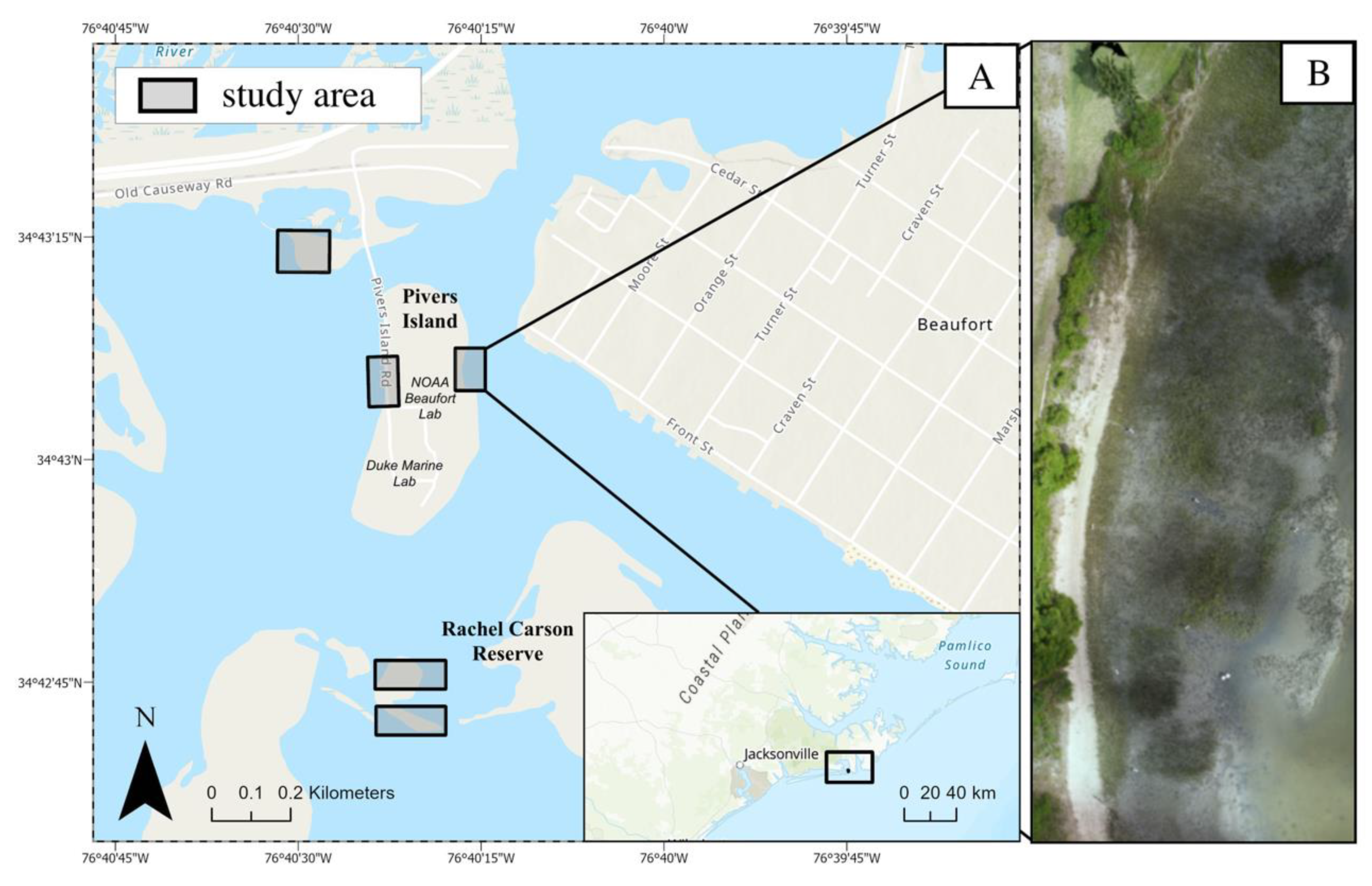
2.1. Study Area

Five Spartina alterniflora dominated salt marshes on the coast of Beaufort, North Carolina were selected to reflect a variety of marsh vegetation heights. These five sites, over the course of six UAS flights, were used to estimate vegetation height (Figure 1). These areas included three sites on Pivers Island adjacent to the Duke University Marine Lab (DUML) and National Oceanic and Atmospheric Administration (NOAA) Beaufort Lab, as well as two sites in the Rachel Carson Reserve, part of the North Carolina National Estuarine Research Reserve.

2.2. Data Collection

2.2.1. UAS Flight Information

Aerial surveys were conducted with a DJI Spreading Wings S900 Hexacopter equipped with a Sony alpha 6000 24.3 megapixel RGB camera and a 1280 × 960 pixel MicaSense RedEdge multispectral sensor. The Sony camera collected full resolution RGB images in RAW format and the radiometrically calibrated RedEdge sensor simultaneously collected multispectral (Red, Green, Blue, Red Edge and Near Infrared) images in RAW format [33]. Flights were conducted along pre-programmed perpendicular survey lines with approximately 75–80% overlap, both laterally and longitudinally, from altitudes ranging from 30–50 m. All images were collected from a nadir perspective. The number of images collected and total flight time varied, depending on the marsh area at each site. For example, for the site displayed in Figure 1, 470 images were collected over a flight time of 11 minutes to cover an area of 0.004 km². Surveys were conducted at low tide according to tidal data from Beaufort Duke Marine Lab Station, Beaufort ID 8656483. Low tide conditions were necessary to ensure that the vegetation was not inundated by water, which would potentially interfere with bare earth models. Flights were conducted during the summer season over a three-month period from July 2018 to September 2018 and a two-month period from June 2019 to July 2019.

2.2.2. Ground Control Points

Incorporating points of known locations is important for high accuracy georeferencing of the UAS mapping data [34]. Ground Control Points (GCPs) were used to improve the 3D position accuracy (X, Y, Z) of the digitized marsh surface. The GCPs used in this study were 0.0929 m² high-density polyurethane black and white checkerboard tiles, which were evenly distributed around the survey area. GCP location was recorded with an Emlid Reach RS Real-Time Kinematic Global Positioning System (RTK-GPS) and subsequently incorporated into the image processing in the software program Pix4D mapper by partial-automation. Horizontal data were referenced to the World Geodetic Datum 1984 (WGS 1984) Universal Transverse Mercator (UTM) Zone 18N, and vertical data were referenced to the North American Vertical Datum established in 1988 (NAVD88).

2.2.3. Stem Height and Vertical Profile Validation

Field measurements of stem heights provided true ground data with which to compare the drone-derived vegetation heights. The field method used to collect true vegetation height data was adapted from the work of Currin et al. [4]. Square quadrats sized 1 m × 1 m were placed across the marsh. Depending on the size of the marsh being surveyed, between seven and 32 quadrats were measured. Sampling quadrats were distributed in a stratified sampling pattern to encompass a wide range of S. alterniflora heights. Within a 1 m² quadrat, the heights of ten stems along the shore-perpendicular middle line of the plot were recorded. Within the 1 m² plot, stem density was measured within a 0.25 m² quadrat. A GPS point was taken with an Emlid Reach RS in the center of each plot to geolocate the manually measured data for comparison with drone-derived vegetation height data.

Previous studies have demonstrated that vegetation height predictions can serve as a proxy for Above Ground Biomass (AGB) [18]. To confirm this, an equation was used to transform manual vegetation height measurements to observed AGB, and this data were regressed against drone-derived predicted vegetation height. Calculations of AGB were derived from an estimate of the vegetation stem dry weight (g) and true field measurements of the stem count and average vegetation height within a sampling plot.

Estimates of the vegetation stem dry weight (g) were derived from Equation (1), a relationship developed by Davis et al. (Davis, Currin, O’Brien, Raffenburg, & Davis, 2015):

y = 0.000005x³ + 0.0003x² + 0.0008x,

(1)

where y is the dry weight (g) of one S. alterniflora plant stem and x is the stem height (cm) of that plant, represented by the average true stem height within a given 1 m² sampling quadrat. Using field data and the results of Equation (1), AGB was calculated using Equation (2):

a = (y*w)/z,

(2)

where a represents the AGB (g/m²), y is the dry weight of one plant stem (g) derived from Equation (1), w is the true stem count associated with the sampling quadrat, and z is the area of the sampling quadrat (m²) in which the stem count was measured. Predicted vegetation height was regressed against the estimated AGB calculated from Equation (2) to understand if a drone-derived vegetation height model created using this framework can serve as an indicator for AGB.

Given that S. alterniflora stems tend to decrease in lateral surface area with an increase in vertical height (leaf blades thin at extremity), the lateral canopy density likely decreases with vertical height (leaf density is greater closer to the ground). Therefore, the UAS-SfM workflow may underestimate plant height as the canopy may be too sparse at the plant tips. To assess if the vegetation height estimates from UAS-SfM fall within this vertical profile of S. alterniflora, methods developed by Lemein et al. (2015), and Neumeier (2005) were modified to capture imagery of the salt marsh lateral vegetation area [35,36]. To compute the lateral vegetation area, or lateral obstruction, a Canon EOS M was mounted to a PVC frame that held a 1.5 m tall mirror at a 45° angle. The camera was centered on the mirror to capture photos of the reflected marsh profile. A white board was placed 25 cm horizontally from the base of the PVC apparatus to provide a solid background (Figure 2) and plots were shaded to eliminate shadowing on the background. A total of 16 plots were imaged in this way, and the resulting imagery was analyzed using pixel analysis with Python and the OpenCV library. By identifying the vegetated pixels, the distribution of the vegetated area at increasing heights could be calculated. To understand where the drone-derived vegetation height predictions fell on the vegetation’s vertical profile, predicted vegetation heights were plotted against the true lateral vegetation area at the sampling quadrat. From these curves, the proportion of vegetation area encompassed by predictions was calculated.

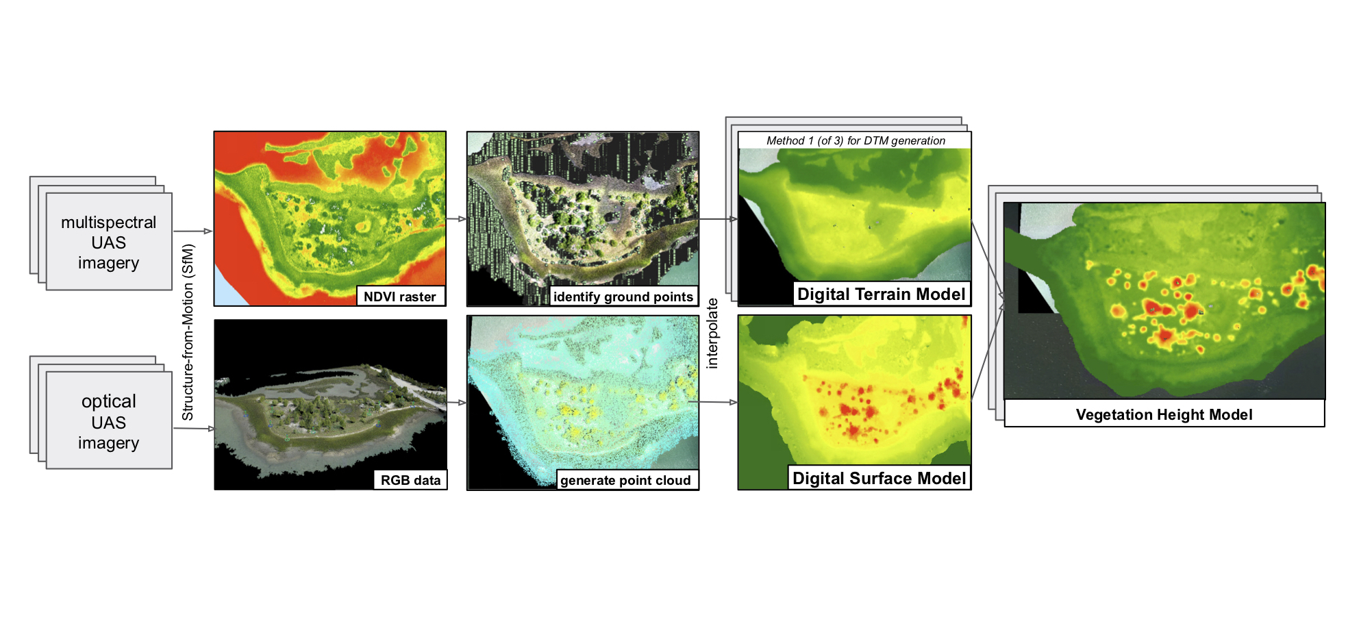
2.3. UAS Imagery Processing

Images collected by the UAS were processed through Pix4D photogrammetry software to generate RGB orthomosaics and multispectral indices. The resultant rasters had a Ground Sampling Distance (GSD) of approximately 0.75 cm/pixel (mean = 0.74, SD = 0.41) for RGB imagery and 2.5 cm/pixel (mean = 2.42, SD = 1.15) for multispectral imagery. GCP data were incorporated with a semi-automated approach requiring a visual identification of each GCP center in at least five different images. Point cloud creation was executed with optimal point density and four minimum image matches. From multispectral imagery, a raster for each spectral index was generated. The Normalized Difference Vegetation Index (NDVI), one of the rasters generated in Pix4D, was used to identify vegetated areas. The NDVI has been widely used to understand the presence and health of vegetation [37]. A point cloud containing 3D positional information was generated from the RGB imagery and exported as a LAS file for compatibility with ArcGIS Pro Mapping Software version 2.0.1 (ESRI Inc., Redlands, CA, USA).

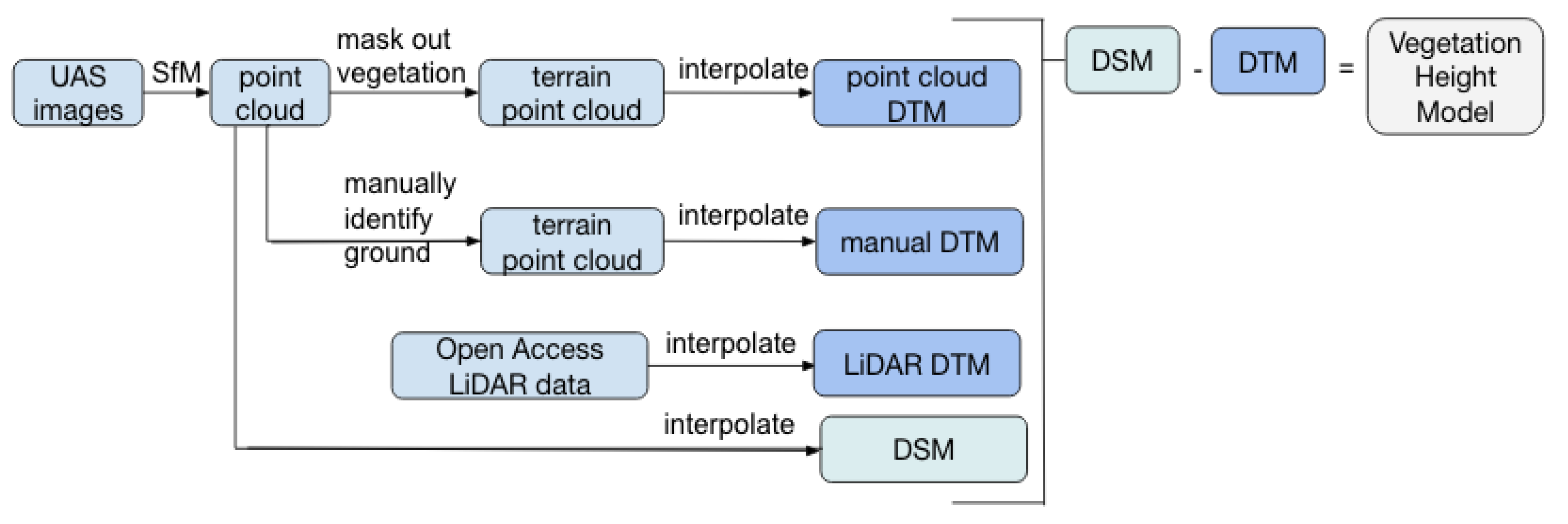
2.4. Drone-Derived Vegetation Height

A Digital Surface Model (DSM) was constructed by connecting the RGB point cloud points based on their 3D position. The conversion of points to a continuous surface required interpolation between points. Previous studies have used an Inverse Distance Weighted (IDW) interpolation technique to convert UAS-SfM point clouds to raster surfaces, and a review of common interpolation methods demonstrates that IDW has the lowest mean error when rasterizing LiDAR point clouds of vegetated landscapes [32,38]. IDW connects points by assuming that points closer to one another are more similar in elevation, or Z-value, than points farther away [39]. IDW was used to connect and smooth all points in the point cloud into a single rasterized DSM at resolution 0.5 m/pixel representing the tops of the plant stems in vegetated areas and ground terrain in non-vegetated areas.

A Digital Terrain Model (DTM) represents the bare earth elevation of the salt marsh. Three DTMs were constructed using three different methods: (1) interpolating between ground points identified with the NDVI, (2) interpolating between manually identified ground points, and (3) interpolating through LiDAR-derived terrain points.

The first method identified and removed vegetated points from the RGB point cloud based on their NDVI values. High values of NDVI represent vegetated areas and low values represent ground, or non-vegetated, areas. To distinguish between these two groups, an NDVI threshold of 0.3 was established based on an assessment of NDVI values across the marsh. The analyst identified ground points (n = 20–30) by visual inspection of the RGB orthomosaics at each site, and the corresponding NDVI value at each of these points was extracted. Though NDVI values for ground points varied within and between sites, the approximate minimum NDVI value observed for ground points was used as a threshold and points with NDVI values greater than this threshold (NDVI = 0.3) were considered vegetated and removed. Choosing the minimum NDVI value for ground points reduced the possibility of mis-identifying vegetated points as ground, which could impact the terrain model substantially. The remaining points were interpolated using IDW to generate a DTM raster at resolution 0.5 m/pixel. This workflow was packaged into a python script to be interfaced with ArcGIS. Using the inputs, a point cloud LAS file and NDVI raster (GSD = ~2.5 cm/pixel) from photogrammetry software, the tool exported a rasterized terrain model.

The second method required manual identification of the ground points using the orthomosaic, an image of the entire site generated by stitching individual sites together. Approximately 20–30 non-vegetated ground points were manually chosen at each site and the height of the DSM at these locations was extracted. Compared to the point cloud method (n > 1,000,000 points), and the LiDAR method (n > 5000 points), the manual method used very few terrain points. Though IDW was used for the two other methods, IDW was not appropriate for the manual method DTM interpolation as it works best with a high density of points. The DTM was therefore interpolated using a Trend interpolation method, which rather than capturing fine scale variation, captures coarse-scale variation by fitting a third order polynomial function to the points. This interpolation method was used because it generates gradually varying surfaces and can be constructed from a low density of sample points.

The third method used a Topobathy LiDAR terrain model from the 2014 National Oceanic and Atmospheric Administration’s (NOAAs) National Geodetic Survey (NGS) Post Hurricane Sandy Topobathymetric LiDAR data. Rasterized LiDAR ground returns were generated at 0.5 m/pixel from Low Water missions flown on 8–9 January 2014. The data were accessed using the National Oceanic and Atmospheric Administration’s Data Access Viewer [40].

A model of the marsh vegetation height was calculated as the difference between the plant tips, represented by the DSM, and the ground surface beneath the vegetation, represented by the DTM (Figure 3). This Vegetation Height Model was generated at 0.5 m/pixel resolution.

2.5. Comparing Predicted to Observed Data

To understand the reliability of the drone-derived vegetation heights, predicted values were compared to observed values measured in the field. The observed stem heights were summarized within a sampling quadrat by taking the mean of the ten measured stem heights. Predicted vegetation height was derived from extracting the mean value of the vegetation height raster within the area of a sampling quadrat in ArcGIS. The area of each quadrat was digitally recreated by generating 1 m² polygons centered at the GPS points taken at a sampling quadrat’s center.

2.6. Vegetation Height Prediction Validation

To understand the consistency with which the drone-derived vegetation heights were being predicted across different stem heights, a linear model was fit to observed and computed data for each DTM creation method. To test the consistency of the linear relationship between observed and computed data across all sampling locations, all observations (n = 139) for each method were randomly split into training and testing sets using ten-fold cross-validation [41,42]. Ten randomly generated folds were created in the data, and a linear model was generated based on the training set, represented by nine of the ten folds, and tested for its ability to predict computed height for the tenth fold. This process was performed ten times iteratively, using all of the data folds as both training and testing. The testing error was averaged, and the distribution of these mean errors was visualized for each of the ten iterations. Advantages of k-fold cross-validation include a reduced dependency on a single testing set to determine model error and a more robust estimate of model error by using 10 different training/testing splits rather than one [43].

2.7. Transformation

While each of the models predicted stem height with consistency, these predictions generally underestimated true stem heights. In order to generate a model that predicts vegetation height consistently and accurately, a vegetation height transformation was developed. To do this, the slope and intercept parameters for the linear regression of computed (predicted) vs. observed (true) stem height were extracted. These parameters were used to transform computed vegetation height predictions to have a 1:1 linear relationship with observed data.

3. Results

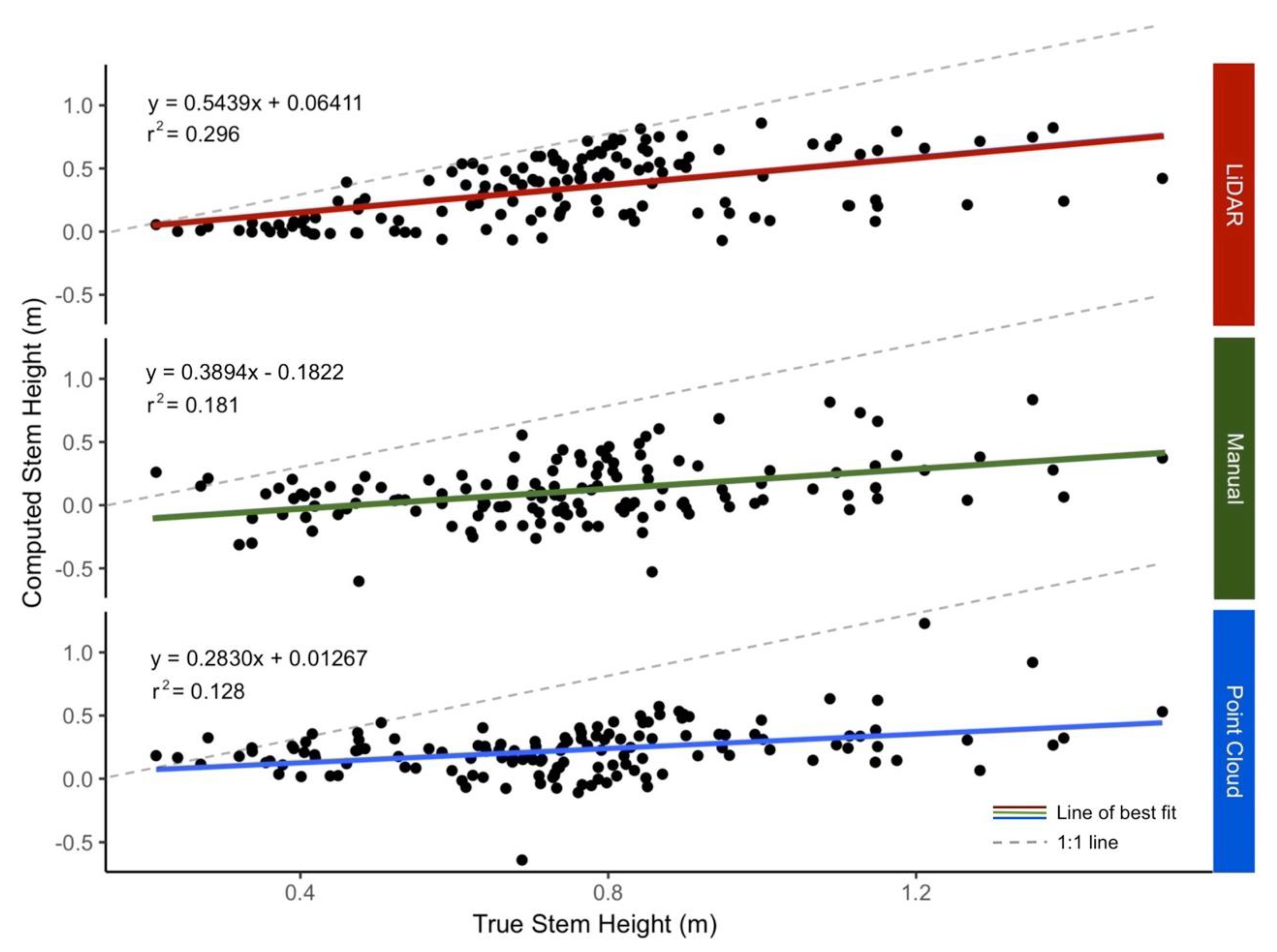
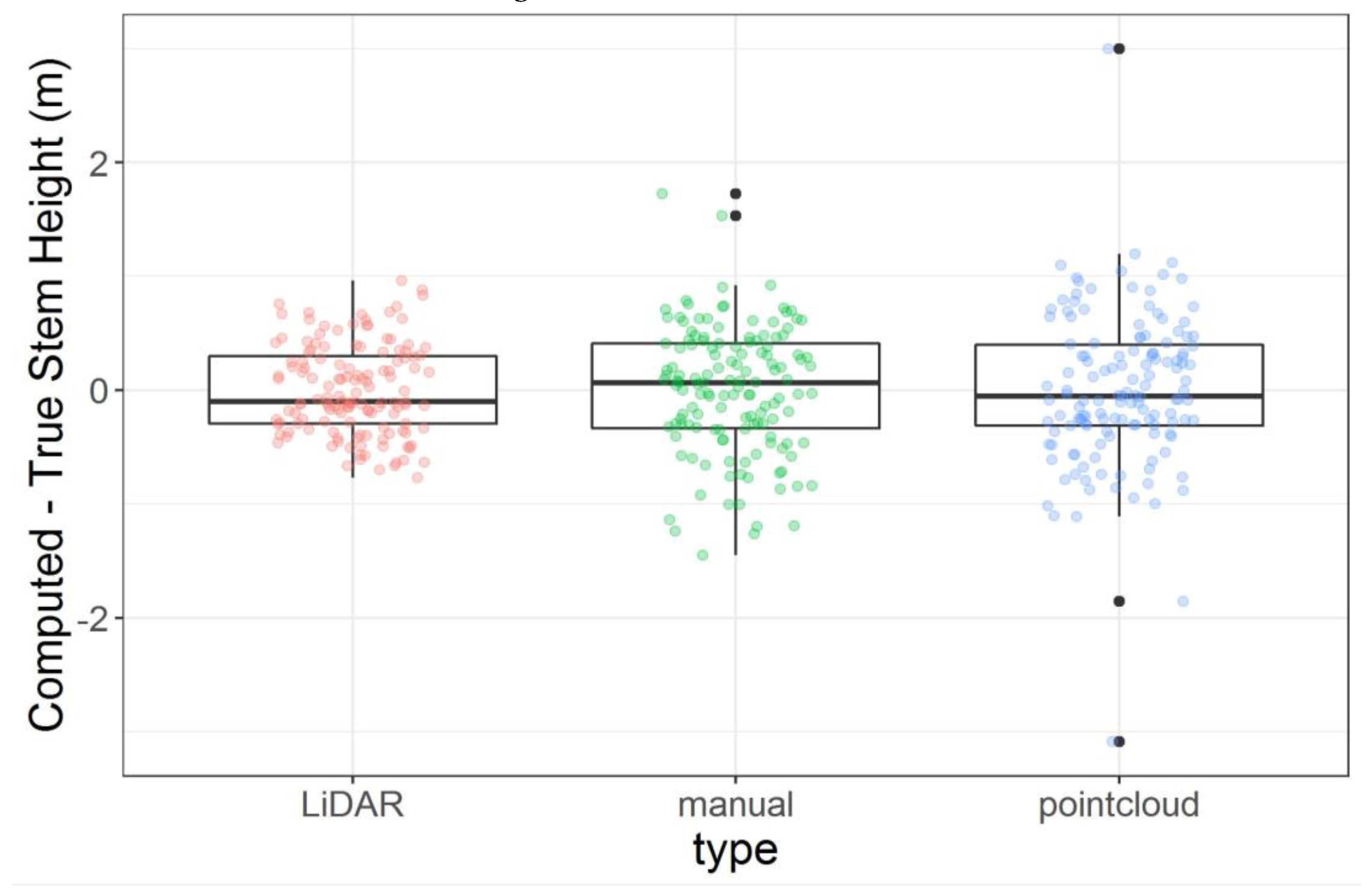
3.1. Drone-Derived Vegetation Height

All three computed vegetation height methodologies (1. point cloud, 2. manual, 3. LiDAR) demonstrated significant linear relationships between the predicted vegetation height and the true observed vegetation height data. The strength of the linear fit varied across the three methodologies: the LiDAR method showed the strongest fit (r² = 0.296), while the point cloud method demonstrated the weakest fit (r² = 0.128) (Figure 4). The small slopes values of the regression equations demonstrated that all three methods were under-predicting vegetation height proportionally, missing more absolute vegetation at higher stem heights (Figure 4).

Residuals from the linear regression models developed in 10-fold cross-validation were calculated for each of the vegetation height prediction methods (1. point cloud, 2. manual, 3. LiDAR). Cross-validation results before transformation show that the point cloud method demonstrated the lowest Mean Squared Error (MSE), with a mean MSE of about 0.025 m². LiDAR and manual methods had comparable mean MSE (~0.045 m²), but the manual method showed considerably greater variability in the model MSE. The maximum difference in the mean model MSE across the three methodologies was approximately 0.02 m² (Figure 5).

Transformation

After transformation, the LiDAR method demonstrated the best accuracy with a mean of −2.24 × 10⁻¹⁶ ± 0.40 m. The manual method had a mean of 1.67 × 10⁻¹⁶ ± 0.56 m and the point cloud method had a mean of −3.01 × 10⁻¹⁶ ± 0.67 m (Figure 6).

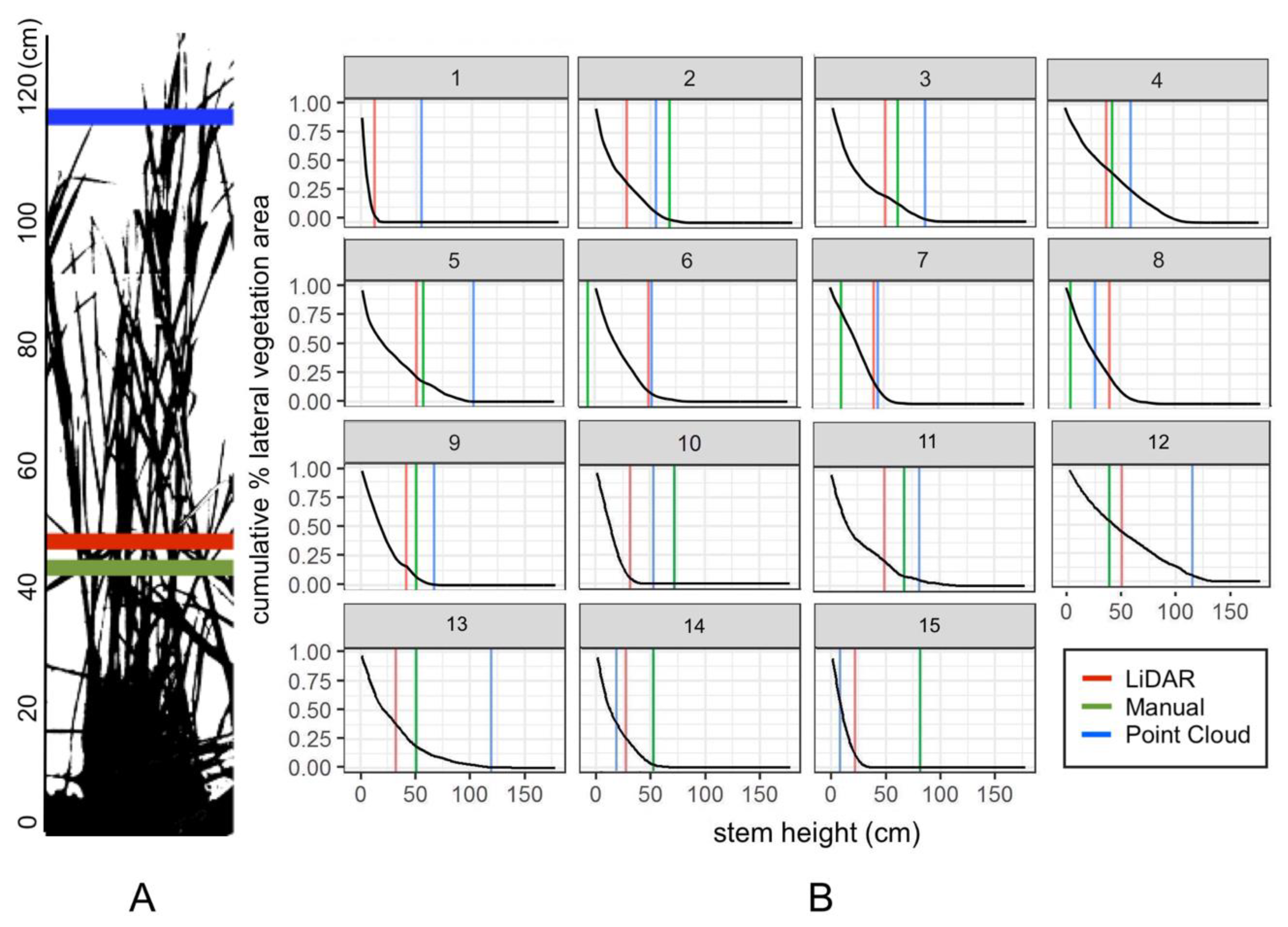
3.2. Biomass Proxy and Lateral Area

All subsequent calculations exploring drone-derived vegetation heights were based on transformed data. To understand if drone-derived vegetation height can be used as a proxy for AGB, predicted height was regressed against the estimated AGB (derived from Equation (2)) for each DTM construction method. AGB was computed using field-based measurements of stem heights as inputs to the height-weight regression for S. alterniflora developed by Davis et al. (2015). Vegetation height models generated from LiDAR, manual, and point cloud methods all demonstrate significant correlations (Pearson’s correlation analysis) with estimated AGB (Figure 7).

The cumulative proportion of the lateral vegetation area at increasing stem heights was calculated from the image analysis of vertical profile validation images (Section 2.2.3) and plotted. The corresponding predicted vegetation height for each of the three methods was displayed to show the relative proportion of the lateral vegetation area captured in each plot (Figure 8).

By comparing the proportion of lateral vegetation area missed by predictions pre-transformation and post-transformation, it is clear that the drone-derived vegetation height model transformation successfully captured most of the lateral vegetation area. Across all three methods, the mean percentage of vegetation area captured increased by at least 35% after transformation. The point cloud method captured the greatest proportion of vegetation area, on average, accounting for a mean 86.0 ± 18.3% of true lateral vegetation area. The LiDAR methods captured a mean of 76.7 ± 13.0% area, on average. The manual method captured 74.2 ± 30.2% area and its high standard deviation indicated its large variance (

Table 1. Proportion of true lateral vegetation area encompassed by predictions for pre-transformed and post-transformed vegetation height predictions.

Method	Pre-Transformation Proportion of Area Encompassed	Post-Transformation Proportion of Area Encompassed
Point cloud	0.485 ± 0.211	0.860 ± 0.183
Manual	0.231 ± 0.196	0.742 ± 0.302
LiDAR	0.395 ± 0.103	0.767 ± 0.130

).

4. Discussion

4.1. Drone-Derived Vegetation Height

In the present study, all three vegetation height prediction methods produced significant linear relationships (p < 0.0001) between observed and expected data but with low r² values (r² = 0.128–0.296) (Figure 4). However, this finding is consistent with a previous study by Kulawardhana et al. using LiDAR returns to quantify the vegetation height of S. alterniflora dominated salt marshes in Texas where the linear regression of the mean vegetation height and field measurements produced an r² of 0.34 [14]. Variation was also assessed by looking at the Mean Squared Error (MSE), which demonstrated small differences across the three methods (MSE 0.025–0.045) (Figure 5). While this suggests that the three models were very similar in vegetation height predictions, there are trade-offs associated with each model including the financial cost of purchasing multispectral sensors, variations in computing costs, and the limited availability of recent high-resolution LiDAR DEMs.

For all models, the regression slopes were substantially smaller than one (m = 0.283–0.544), indicating that vegetation height predictions were consistently underestimated (Figure 4). The low slope suggests that the predicted vegetation heights were being underestimated in a linear pattern, meaning that the difference between field observations and drone-derived vegetation heights increased at higher stem heights.

This is consistent with other studies using LiDAR data to quantify the vegetation height of short herbaceous vegetation. In rangelands, Ritchie et al. (1996) and Weltz et al. (1994) experienced LiDAR underestimations of vegetation height [44,45]. Kulawardhana et al. (2014) underestimated vegetation heights by a mean of 15 cm [14], and Wang et al. (2009) underestimated by 17.7 cm [46]. These results are comparable to drone-derived vegetation height underestimations before transformation (Figure 4).

Underestimations may be explained by the decreasing surface area of S. alterniflora progressing from the plant base to the plant tip (Figure 8). Surveying at a resolution on the scale of centimeters, drone imagery may not be able to identify the tips of the plants. Additionally, S. alterniflora stalks exhibit a slight curvature, as the plant tip slopes over. However, field measurements were made using the traditional method, by holding the plant tip up straight and measuring from plant base to tip. This discrepancy is addressed in the present study by performing a transformation on the data. In similar studies using LiDAR, underestimations are thought to be caused by dense canopies which are difficult to penetrate [14,45,46,47]. This issue may apply to the LiDAR-derived DTM method, but the LiDAR dataset used in this study was derived from post-hurricane imagery in January 2014 as part of NOAA’s post-Hurricane Sandy survey. Seasonally, this would be near minimum biomass, which would reduce vegetation interference and may explain the high accuracy of the LiDAR DTM (Table S1). Marsh density is a consideration for the point cloud method as well, as the DTM would be generated based on fewer ground points within the marsh as identified by NDVI, or manually for dense marshes. DTM accuracy varied across sampling sites which may be attributed to the sites reflecting a range of marsh densities. High terrain differences were seen at the Pivers Island North site, which is characterized by moderately dense and medium-to-high-stemmed S. alterniflora (Figure S1). Further exploration should investigate the impact of stem height and density on the DTM construction capabilities, with the possibility of using winter-season data (like the LiDAR dataset), which would reflect sparser marsh conditions, to create a better DTM and potentially increase the predictive capacity of the UAS-based regression models provided.

When comparing the models using cross-validation before transformation, there were no clear differences among the model mean squared errors (Figure 5). Predicted values were therefore transformed for all three methods and compared to the expected results. When examining the distribution of differences between field observations and drone-derived vegetation heights after transformation, the point cloud method stood out as having several extreme values, two of which demonstrated a difference between predicted and observed data of greater than two meters. It is possible that artifacts in the SfM-generated point cloud were incorporated into the terrain model, resulting in large differences. In the future, to reduce the effects of these extreme values, the point cloud can be cleaned of extreme artifacts first. The manual method also produced two large values greater than one meter (Figure 6), which could potentially be attributed to the sparse points from which the terrain model is interpolated. The manually constructed terrain model is interpolated from only 20–30 points, so it fails to capture local variations. Any steep local changes in terrain elevation would be missed by this method and generate large differences between observed and predicted values. The LiDAR method’s distribution does not have apparent extreme values, perhaps because the LiDAR method derives a terrain model from high-resolution LiDAR data (Figure 6). The high resolution of the LiDAR data may increase the ability of this DTM to capture local variation. Additionally, the LiDAR terrain dataset used in this analysis is from 2014, meaning that it may fail to capture accretion and other terrain changes over time.

Underestimations also are likely generated when the point cloud is smoothed from a group of points to a continuous, rasterized surface. The tool used to generate the DSM used all points in the point cloud to generate a continuous surface and incorporated a smoothing filter that may have smoothed over plant tips. Filtering the point cloud to only include local maximums, representing the plant tips, could greatly improve the DSM and reduce the effect of smoothing. However, identifying local maximums in a dense point cloud across a large area may cost a great deal of additional computer processing power and time.

A limitation to this analysis is the coarse resolution of the drone-derived vegetation height model. The vegetation height model can distinguish between vegetated areas, having a non-zero vegetation height, and non-vegetated areas, having a zero-centimeter vegetation height, across different 0.25 m² plots. Within a 0.25 m² plot, however, this analysis fails to account for partially vegetated plots. For this reason, the resolution with which marsh transgression or progression can be detected is likely on the order of 0.5 m². It is predicted that if marsh coverage changes by 0.5 m² or more, at least one 0.25 m² plot will change from vegetated to non-vegetated, or vice versa, and the drone-derived vegetation height will reflect a vegetation height difference.

An advantage to this framework is the flexibility of the model. For this analysis, a reduced processing burden was favored over increased resolution. However, by gridding the surface model and terrain models to rasters of higher resolution (<0.25 m²), smaller scale changes can perhaps be resolved. More research is needed to determine the appropriate grid size of LiDAR datasets and DSM rasters for optimizing the processing power input and raster model resolution.

4.2. Biomass Proxy and Lateral Area

A significant correlation between drone-derived vegetation height and estimated AGB across all three DTM construction methods indicates that vegetation height models constructed using this framework can potentially be used as a proxy for biomass, but further work would be needed to explore this (Figure 7). It should be noted that high AGB estimates (>2000 g/m²) were observed, and these were characteristic of tall-stemmed sampling plots with moderate stem densities (Figure S2). The Davis et al. (2015) equation (Equation (1)) used to calculate the dry weight of a given S. alterniflora stem reflects an exponential relationship, predicting increasingly higher weights at high stem heights [6]. This relationship was developed on plants 0–1.2 m in height, reflecting a sampling pool that does not encompass the stems of up to 1.5m tall found in this study. Predicted dry weights (g) of these tall stems, while outside the Davis et al. (2015) model, were within the range of measured values obtained by Morris and Haskin (1990) on similar height S. alterniflora stems [48]. All high AGBs were estimated from tall-stemmed plots. Considering the height–weight relationship, the vegetation height of a given ecosystem over time therefore has potential to indicate changes in biomass.

After transformation, the amount of lateral vegetation area encompassed by drone-derived vegetation heights increased by 40–60%. Comparing the three methods, the manual DTM method demonstrates the greatest spread, in some cases nearing 100% lateral vegetation area missed (Table 1). This can perhaps be attributed to the low resolution of the manual method DTM. In areas of the marsh that have steep changes in ground elevation, like the high marsh of our study sites, the manual method may miss the vegetation entirely. However, in short stem plots (<50 cm), the manual method appears to capture the most lateral vegetation area (Figure 8a). This may be a result of low stem plots being located in sparse areas of the marsh. Sparse areas, containing more visible ground, would enable manual identification of ground points and demonstrate higher accuracy, whereas dense plots in the middle of the marsh might be farther away from a chosen ground point and have increased error. For these high stem plots (>90 cm), the point cloud method tends to encompass the most lateral vegetation area relative to the other two methods (Figure 8a). The point cloud method also encompasses the greatest percent of lateral vegetation area on average (86.0 ± 18.3%). Perhaps this is because the point cloud DTM is constructed from a much higher density of ground points than the manual method. While the LiDAR DTM shares this high density of ground points, it fails to represent the marsh in its present state: as the dataset is from 2014, it does not capture potential accretion or erosion over the past five years. The low density of open access LiDAR datasets over time also presents a problem for monitoring this ecosystem.

Previous studies have used red and Near-Infrared (NIR) bands and vegetation indices derived from these bands to quantify salt marsh vegetation biomasses, predicting biomasses with approximately 60–90% accuracy [17,47]. Relying on spectral indices alone means that these studies can face a “saturation problem”, where spectral bands cannot detect changes in biomass beyond a threshold of canopy density [49,50]. The framework presented in this study can potentially be used to improve these spectral methods of biomass quantification by providing additional data on canopy height and structure [50].

Moreover, the vegetation height data derived from this method can be used to inform the resilience of a given marsh ecosystem to wave energy and storm surge. In previous studies, vegetation height has been correlated with the ability of vegetation to dissipate wave energy [51]. Lateral vegetation area is predicted with approximately 75–85% accuracy in this study and can be used to complement biomass estimates derived from remote sensing (Figure 8). By producing accurate models of vegetation height, this study has the potential to improve our understanding of current and future ecosystem health from remotely sensed spectral data without SfM, which is recorded in two dimensions and fails to capture marsh canopy height or structure.

5. Conclusions

While the surface models, or DSMs, representing plant tips were all constructed by interpolating through the SfM-generated point cloud, bare-earth models, or DTMs, were constructed using three methods: 1. interpolating between NDVI-identified ground points in the SfM point cloud, 2. interpolating between manually identified ground points, and 3. using LiDAR-derived digital elevation models. Raster subtraction between these two surfaces (DSM–DTM) was performed to generate a Vegetation Height Model at 0.5 m² resolution. Underpredictions of vegetation height resulting from these methods necessitated a linear transformation which was developed and tested using 10-fold cross-validation, producing predictions with smaller error.

Comparing the three DTM methods after transformation, the point cloud method demonstrated comparable accuracy to that of the LiDAR method, but predicted vegetation heights with the greatest consistency, demonstrated by the low MSE of 10-fold cross-validation. However, the point cloud method requires multi-spectral data which are often more expensive than optical data and may require an entirely separate sensor. The manual method eliminates the need for multispectral data but requires user input and predicts with a larger error relative to the other two methods. The LiDAR method therefore provides a cost-effective, more streamlined alternative. However, this method sacrifices some of the accuracy and precision of the point cloud method and relies on the availability of readily accessible LiDAR data.

This study lays the groundwork for applying UAS to generate vegetation height measurements across the marsh ecosystem and provides a framework for using UAS to estimate the AGB of emergent vegetation, which may have important implications for blue carbon estimations. It is anticipated that future endeavors will capitalize on advances in UAS technology (platforms, sensors, and software) to build on this work to explore adjustments to the methodology (e.g., winter season flights for DTM data) and improve the accuracy of the regressions and biomass estimations. This work minimizes anthropogenic impacts to the salt marsh ecosystem, reduces the cost of labor required for manual measurements, and greatly expands the scale of assessment.

References

1. Morris, J.T.; Sundareshwar, P.V.; Nietch, C.T.; Kjerfve, B.; Cahoon, D.R. Responses of Coastal Wetlands to Rising Sea Level. Ecology 2002, 83, 2869–2877. [Google Scholar] [CrossRef]
2. Meixler, M.S.; Kennish, M.J.; Crowley, K.F. Assessment of Plant Community Characteristics in Natural and Human-Altered Coastal Marsh Ecosystems. Estuaries Coasts 2018, 41, 52–64. [Google Scholar] [CrossRef]
3. Marinucci, A.C. Trophic importance of Spartina alterniflora production and decomposition to the marsh-estuarine ecosystem. Biol. Conserv. 1982, 22, 35–58. [Google Scholar] [CrossRef]
4. Currin, C.A.; Delano, P.C.; Valdes-Weaver, L.M. Utilization of a citizen monitoring protocol to assess the structure and function of natural and stabilized fringing salt marshes in North Carolina. Wetl. Ecol. Manag. 2008, 16, 97–118. [Google Scholar] [CrossRef]
5. Barbier, E.B.; Hacker, S.D.; Kennedy, C.; Koch, E.W.; Stier, A.C.; Silliman, B.R. The value of estuarine and coastal ecosystem services. Ecol. Monogr. 2011, 81, 169–193. [Google Scholar] [CrossRef]
6. Davis, J.L.; Currin, C.A.; O’Brien, C.; Raffenburg, C.; Davis, A. Living Shorelines: Coastal Resilience with a Blue Carbon Benefit. PLoS ONE 2015, 10, e0142595. [Google Scholar] [CrossRef]
7. Zhou, Z.; Yang, Y.; Chen, B. Estimating Spartina alterniflora fractional vegetation cover and aboveground biomass in a coastal wetland using SPOT6 satellite and UAV data. Aquat. Bot. 2018, 144, 38–45. [Google Scholar] [CrossRef]
8. Byrd, K.B.; O’Connell, J.L.; Di Tommaso, S.; Kelly, M. Evaluation of sensor types and environmental controls on mapping biomass of coastal marsh emergent vegetation. Remote Sens. Environ. 2014, 149, 166–180. [Google Scholar] [CrossRef]
9. Eon, R.S.; Goldsmith, S.; Bachmann, C.M.; Tyler, A.C.; Lapszynski, C.S.; Badura, G.P.; Osgood, D.T.; Brett, R. Retrieval of salt marsh above-ground biomass from high-spatial resolution hyperspectral imagery using PROSAIL. Remote Sens. 2019, 11, 1385. [Google Scholar] [CrossRef] [Green Version]
10. Neckles, H.; Dione, M. Regional Standards to Identify and Evaluate Tidal Wetland Restoration in the Gulf of Maine; Wells National Estuarine Research Reserve: Wells, ME, USA, 1999. [Google Scholar]
11. Nolte, S.; Esselink, P.; Smit, C.; Bakker, J.P. Herbivore species and density affect vegetation-structure patchiness in salt marshes. Agric. Ecosyst. Environ. 2014, 185, 41–47. [Google Scholar] [CrossRef]
12. Elzinga, C.; Salzer, D.; Willoughby, J. Measuring & Monitering Plant Populations; Bureau of Land Management: Washington, DC, USA, 1998.
13. Minchinton, T.E.; Shuttleworth, H.T.; Lathlean, J.A.; McWilliam, R.A.; Daly, T.J. Impacts of Cattle on the Vegetation Structure of Mangroves. Wetlands 2019, 1–9. [Google Scholar] [CrossRef]
14. Kulawardhana, R.W.; Popescu, S.C.; Feagin, R.A. Fusion of lidar and multispectral data to quantify salt marsh carbon stocks. Remote Sens. Environ. 2014, 154, 345–357. [Google Scholar] [CrossRef]
15. Roughgarden, J.; Running, S.W.; Matson, P.A. What Does Remote Sensing Do for Ecology? Ecology 1991, 72, 1918–1922. [Google Scholar] [CrossRef]
16. Gross, M.F.; Hardisky, M.A.; Klemas, V.; Wolf, P.L. Quantification of Biomass of the Marsh Grass Spartina alterniflora Loisel Using Landsat Thematic Mapper Imagery. Photogramm. Eng. Remote Sens. 1987, 53, 1577–1583. [Google Scholar]
17. Zhang, M.; Ustin, S.L.; Rejmankova, E.; Sanderson, E.W. Monitoring Pacific coast salt marshes using remote sensing. Ecol. Appl. 1997, 7, 1039–1053. [Google Scholar] [CrossRef]
18. Klemas, V. Remote Sensing of Coastal Wetland Biomass: An Overview. J. Coast. Res. 2013, 290, 1016–1028. [Google Scholar] [CrossRef]
19. Montané, J.M.; Torres, R. Accuracy Assessment of Lidar Saltmarsh Topographic Data Using RTK GPS. Photogramm. Eng. Remote Sens. 2006, 72, 961–967. [Google Scholar] [CrossRef]
20. Hladik, C.; Alber, M. Accuracy assessment and correction of a LIDAR-derived salt marsh digital elevation model. Remote Sens. Environ. 2012, 121, 224–235. [Google Scholar] [CrossRef]
21. Collin, A.; Long, B.; Archambault, P. Merging land-marine realms: Spatial patterns of seamless coastal habitats using a multispectral LiDAR. Remote Sens. Environ. 2012, 123, 390–399. [Google Scholar] [CrossRef]
22. Moudrý, V.; Gdulová, K.; Fogl, M.; Klápště, P.; Urban, R.; Komárek, J.; Moudrá, L.; Štroner, M.; Barták, V.; Solský, M. Comparison of leaf-off and leaf-on combined UAV imagery and airborne LiDAR for assessment of a post-mining site terrain and vegetation structure: Prospects for monitoring hazards and restoration success. Appl. Geogr. 2019, 104, 32–41. [Google Scholar] [CrossRef]
23. Ullman, S. The interpretation of structure from motion. Proc. R. Soc. Lond. 1979, 203, 405–426. [Google Scholar] [CrossRef] [PubMed]
24. Fonstad, M.A.; Dietrich, J.T.; Courville, B.C.; Jensen, J.L.; Carbonneau, P.E. Topographic structure from motion: A new development in photogrammetric measurement. Earth Surf. Process. Landf. 2013, 38, 421–430. [Google Scholar] [CrossRef] [Green Version]
25. Hayakawa, Y.; Obanawa, H. A study of Japanese landscapes using structure from motion derived DSMs and DEMs based on historical aerial photographs: New opportunities for vegetation monitoring and diachronic geomorphology. Geomorphology 2015, 242, 11–20. [Google Scholar] [CrossRef] [Green Version]
26. Kalacska, M.; Chmura, G.L.; Lucanus, O.; Bérubé, D.; Arroyo-Mora, J.P. Structure from motion will revolutionize analyses of tidal wetland landscapes. Remote Sens. Environ. 2017, 199, 14–24. [Google Scholar] [CrossRef]
27. Dandois, J.; Olano, M.; Ellis, E.; Dandois, J.P.; Olano, M.; Ellis, E.C. Optimal Altitude, Overlap, and Weather Conditions for Computer Vision UAV Estimates of Forest Structure. Remote Sens. 2015, 7, 13895–13920. [Google Scholar] [CrossRef] [Green Version]
28. Wallace, L.; Lucieer, A.; Malenovskỳ, Z.; Turner, D.; Vopěnka, P. Assessment of forest structure using two UAV techniques: A comparison of airborne laser scanning and structure from motion (SfM) point clouds. Forests 2016, 7, 62. [Google Scholar] [CrossRef] [Green Version]
29. Cunliffe, A.M.; Brazier, R.E.; Anderson, K. Ultra-fine grain landscape-scale quantification of dryland vegetation structure with drone-acquired structure-from-motion photogrammetry. Remote Sens. Environ. 2016, 183, 129–143. [Google Scholar] [CrossRef] [Green Version]
30. Goetz, S.; Dubayah, R. Advances in remote sensing technology and implications for measuring and monitoring forest carbon stocks and change. Carbon Manag. 2011, 2, 231–244. [Google Scholar] [CrossRef]
31. Lefsky, M.A.; Cohen, W.B.; Harding, D.J.; Parker, G.G.; Acker, S.A.; Gower, S.T. Lidar remote sensing of above-ground biomass in three biomes. Glob. Ecol. Biogeogr. 2002, 11, 393–399. [Google Scholar] [CrossRef] [Green Version]
32. Sturdivant, E.J.; Lentz, E.E.; Thieler, E.R.; Farris, A.S.; Weber, K.M.; Remsen, D.P.; Miner, S.; Henderson, R.E.; Sturdivant, E.J.; Lentz, E.E.; et al. UAS-SfM for Coastal Research: Geomorphic Feature Extraction and Land Cover Classification from High-Resolution Elevation and Optical Imagery. Remote Sens. 2017, 9, 1020. [Google Scholar] [CrossRef] [Green Version]
33. RedEdge-MX—MicaSense. Available online: https://www.micasense.com/rededge-mx (accessed on 24 June 2019).
34. Harwin, S.; Lucieer, A. Assessing the accuracy of georeferenced point clouds produced via multi-view stereopsis from Unmanned Aerial Vehicle (UAV) imagery. Remote Sens. 2012, 4, 1573–1599. [Google Scholar] [CrossRef] [Green Version]
35. Lemein, T.; Cox, D.; Albert, D.; Mori, N. Accuracy of optical image analysis compared to conventional vegetation measurements for estimating morphological features of emergent vegetation. Estuar. Coast. Shelf Sci. 2015, 155, 66–74. [Google Scholar] [CrossRef]
36. Neumeier, U. Quantification of vertical density variations of salt-marsh vegetation. Estuar. Coast. Shelf Sci. 2005, 63, 489–496. [Google Scholar] [CrossRef]
37. Adam, E.; Mutanga, O.; Rugege, D. Multispectral and hyperspectral remote sensing for identification and mapping of wetland vegetation: A review. Wetl. Ecol. Manag. 2010, 18, 281–296. [Google Scholar] [CrossRef]
38. Su, J.; Bork, E. Influence of Vegetation, Slope, and Lidar Sampling Angle on DEM Accuracy. Photogramm. Eng. Remote Sens. 2006, 72, 1265–1274. [Google Scholar] [CrossRef]
39. How Inverse Distance Weighted Interpolation Works—ArcGIS Pro | ArcGIS Desktop. Available online: https://pro.arcgis.com/en/pro-app/help/analysis/geostatistical-analyst/how-inverse-distance-weighted-interpolation-works.htm (accessed on 27 June 2019).
40. National Geodetic Survey, 2020: 2014 NOAA Post Hurricane Sandy Topobathymetric LiDAR Mapping for Shoreline Mapping. Available online: https://inport.nmfs.noaa.gov/inport/item/48141 (accessed on 30 July 2019).
41. Efron, B.; Tibshirani, R. Cross-Validation and the Bootstrap: Estimating the Error Rate of a Prediction Rule; Division of Biostatistics, Stanford University: Stanford, CA, USA, 1995; Volume 92, pp. 548–560. [Google Scholar] [CrossRef]
42. Lek, S.; Guégan, J.F. Artificial neural networks as a tool in ecological modelling, an introduction. Ecol. Model. 1999, 120, 65–73. [Google Scholar] [CrossRef]
43. Viña, A.; Gitelson, A.A.; Nguy-Robertson, A.L.; Peng, Y. Comparison of different vegetation indices for the remote assessment of green leaf area index of crops. Remote Sens. Environ. 2011, 115, 3468–3478. [Google Scholar] [CrossRef]
44. Ritchie, J.C.; Menentif, M.; Weltzj, M.A. Measurements of land surface features using an airborne laser altimeter: The HAPEX-Sahel experiment. Int. J. Remote Sens. 1996, 17, 3705–3724. [Google Scholar] [CrossRef] [Green Version]
45. Weltz, M.A.; Ritchie, J.C.; Fox, H.D. Comparison of laser and field measurements of vegetation height and canopy cover. Water Resour. Res. 1994, 30, 1311–1319. [Google Scholar] [CrossRef]
46. Wang, C.; Menenti, M.; Stoll, M.P.; Feola, A.; Belluco, E.; Marani, M. Separation of ground and low vegetation signatures in LiDAR measurements of salt-marsh environments. IEEE Trans. Geosci. Remote Sens. 2009, 47, 2014–2023. [Google Scholar] [CrossRef]
47. Bartlett, D.S. Quantitative Assessment of Tidal Wetlands Using Remote Sensing. Environ. Manag. 1980, 4, 337–345. [Google Scholar] [CrossRef]
48. Morris, J.T.; Haskin, B. A 5-yr record of aerial primary production and stand characteristics of Spartina alterniflora. Ecology 1990, 71, 2209–2217. [Google Scholar] [CrossRef]
49. Lu, D. The potential and challenge of remote sensing-based biomass estimation. Int. J. Remote Sens. 2006, 27, 1297–1328. [Google Scholar] [CrossRef]
50. Medeiros, S.; Hagen, S.; Weishampel, J.; Angelo, J. Adjusting lidar-derived digital terrain models in coastal marshes based on estimated aboveground biomass density. Remote Sens. 2015, 7, 3507–3525. [Google Scholar] [CrossRef] [Green Version]
51. Tempest, J.A.; Möller, I.; Spencer, T. A review of plant-flow interactions on salt marshes: The importance of vegetation structure and plant mechanical characteristics. Wiley Interdiscip. Rev. Water 2015, 2. [Google Scholar] [CrossRef] [Green Version]
Figure 1. (a) Map of the location of five salt marshes sampled via Unoccupied Aircraft Systems (UAS) for Structure-from-Motion (SfM) photogrammetric vegetation height modeling. (b) Example site orthomosaic derived from SfM-photogrammetry of UAS imagery.
Remotesensing 12 02333 g001
Figure 2. Vertical accuracy apparatus (adapted from Neumeier 2005) [36].
Remotesensing 12 02333 g002
Figure 3. Schematic describing the process of deriving three Digital Terrain Models (DTMs) and one Digital Surface Model (DSM) to generate a vegetation height model.
Remotesensing 12 02333 g003
Figure 4. Computed vs. true regression mapped vegetation height derived from UAS imagery to field-measured true stem heights. The 1:1 line, where computed stem height is equal to true stem height, is displayed for reference. Computed vegetation heights are compared across the point cloud, manual, and Light Detection and Ranging (LiDAR)-derived digital terrain models.
Remotesensing 12 02333 g004
Figure 5. Distribution of regression model mean squared error from 10-fold cross-validation results across three different vegetation height prediction methods.
Remotesensing 12 02333 g005
Figure 6. Distribution of differences between computed (predicted) and true (observed) vegetation height after transformation for each of the three methods: LiDAR, manual, and point cloud.
Remotesensing 12 02333 g006
Figure 7. Predicted vegetation height and Above Ground Biomass (AGB) are significantly correlated using (a) LiDAR, (b) manual, and (c) point cloud terrain model construction methods. AGB is calculated from the height–weight regression developed by Davis et al., stem count and stem height measurements in the field [6]. Predicted vegetation heights are calculated from transformed drone-derived vegetation height estimates.
Remotesensing 12 02333 g007
Figure 8. (a) An example plot is displayed to demonstrate the vertical profile (lateral obstruction) and associated vegetation height predictions across three different DTM generation methods post-transformation. (b) Inverse of the cumulative proportion of grass area encompassed at different stem heights across fifteen sampling quadrats after transformation with corresponding predicted vegetation heights from each of the three methods.
Remotesensing 12 02333 g008