Article

Non-Tidal Mass Variations in the IGS Second Reprocessing Campaign: Interpretations and Noise Analysis from GRACE and Geophysical Models

1
School of Electrical and Electronic Information Engineering, Hubei Polytechnic University, Huangshi 435003, China
2
School of Geodesy and Geomatics, Wuhan University, Wuhan 430079, China
3
State Key Laboratory of Information Engineering in Surveying, Mapping and Remote Sensing, Wuhan University, Wuhan 430079, China
4
GNSS Research Center, Wuhan University, Wuhan 430079, China
*
Author to whom correspondence should be addressed.
Remote Sens. 2020, 12(15), 2477; https://doi.org/10.3390/rs12152477
Submission received: 6 July 2020 / Revised: 24 July 2020 / Accepted: 31 July 2020 / Published: 2 August 2020
(This article belongs to the Section Environmental Remote Sensing)

Abstract

:
Vertical deformations caused by non-tidal mass variations still remain in global navigation satellite system (GNSS) height time series, and can be computed from both Gravity Recovery and Climate Experiment (GRACE) and geophysical models. In this study, we provide a thorough evaluation of the relationships between these different techniques in the global scale by comparing non-tidal vertical deformations from IGS second reprocessing campaign (IG2), GRACE and Global Geophysical Fluid Center (GGFC) solutions, and investigate the noise properties of the GNSS corrected by GRACE solutions and GNSS corrected by GGFC solutions for global stations using optimal noise models. Our results demonstrate that the consistency between seasonal vertical deformations derived from GNSS, GRACE and GGFC is high. When correcting GNSS deformations with GRACE and GGFC solutions, 81% and 73% of the 186 stations have the weight root mean square ( W R M S ) reduction, respectively. The W R M S variations averaged over all stations are −12.3% and −5.6%, respectively for GNSS corrected by GRACE and GNSS corrected by GGFC solutions. The obvious difference occurs in the GNSS corrected by GGFC solutions W R M S increase, with the mean increase value up to 29%, mainly happening to stations located on islands or small peninsulas. In addition, noise properties of the GNSS corrected by GRACE solutions and GNSS corrected by GGFC solutions for global stations are investigated using optimal noise models. After correcting non-tidal loading effects, the solutions of GNSS corrected by GRACE solutions have the lowest noise level, and can occupy 5% of the noise behavior presenting in global stations, while the solutions of GNSS corrected by GGFC solutions can bring more than 5% of the noise into global stations, implying that GRACE correction solutions can present more favorable results when interpreting GNSS non-tidal loading deformations.

Graphical Abstract

1. Introduction

Global navigation satellite system (GNSS) coordinate time series have been widely used in varieties of studies, including global/regional reference frame establishment [1], tectonic deformation monitoring [2], and conducting strain accumulation on sea-level variations [3], glacial isostatic adjustment (GIA), subsidence studies [4]. To provide accurate analysis and appropriate geophysical interpretation, proper eliminations of GNSS data processing errors are required [5,6,7]. Recently, the deformations induced by tidal loading effects have been modeled so accurately that they can be eliminated well during GNSS data processing [8,9,10]. However, non-tidal mass variations normally change very little over typical integration spans (~1 mm), and models for non-tidal effects contain large uncertainty and are usually less accurate. Therefore, non-tidal mass variations are generally suggested by the International Earth Rotation Service (IERS) not to be applied in computing conventional instantaneous positions in GNSS routine data processing procedures [1,11]. The corresponding non-tidal mass variations, which are typically with amplitudes of a few centimeters or less, still remain as signals embedded in the GNSS geodetic coordinate solutions [12,13,14].
Previous studies have established the significance of non-tidal loadings, especially the comprehensive effects induced by changes in atmospheric pressure loading (ATML), continental water storage (CWS), and non-tidal ocean loading (NTOL) [15,16,17]. The non-tidal loading effects can be modeled mainly by two different methods—mass variations from the Gravity Recovery and Climate Experiment (GRACE) satellite mission [18,19,20,21] and solutions from geophysical models (GMs) [22,23]. Many researchers have investigated the relationships among the different techniques, especially in regions with acute environmental mass variations [24,25,26,27,28].
The research of [25] used the homogeneously reprocessed 115 GNSS stations with high quality and GRACE level 2 gravity products from Release 04 from September 2002 to April 2009 for comparisons. Their GNSS data were completely reprocessed in the context of the GGOS-D project (Global Geodetic-Geophysical Observing System-Deutschland) [27], using the Bernese GNSS Software 5.1. The research of [26] compared eleven available solutions from the International GNSSS Service (IGS) Analysis Centers (ACs) with seven GRACE-modeled vertical deformation (VD) solutions based on the globally distributed 110 IGS08/IGS14 core stations, and suggested that GRACE data could provide VD results of good internal consistency, while GNSS solutions from multiple institutions implied large uncertainty. By investigating the predicted deformations with the position time series of 689 globally distributed continuous GNSS stations, research of [13] found that while GNSS vertical deformations are well explained by the model at a global scale, horizontal deformations were systematically underpredicted and out of phase with GNSS station position time series. The research of [13] also determined the estimates of degree-1 spherical harmonic coefficients from GRACE and global GNSS data, and demonstrated improved comparison of the computed deformations from their degree-1 solutions with GNSS measurements, particularly in the horizontal components. In terms of the comparisons between GNSS and GMs. The research of [28] comprehensively compared three different environmental loading methods to estimate surface deformations and correct the nonlinear variations in a set of GNSS weekly height time series. They demonstrated that there are differences remaining in different GMs, and pointed out that for different GMs, the consistency of the VD signals showed discrepancies. Although GNSS, GRACE and GMs can capture the seasonal vertical non-tidal deformations, there are still systematic discrepancies among the three techniques [29,30,31,32]. It has been reported that the weighted root mean square (WRMS) of the GNSS residuals only decrease slightly after subtracting the GRACE-modeled or GM-derived VD series from the GNSS vertical coordinate time series, indicating non-tidal amplitudes differences existing in different techniques [25,31]. Further analysis should be undertaken to analyze the relationships of these techniques and identify the possible reasons for the differences.
GNSS data processing methods and theories have been under continuous refinement in the past 30 years [1,11,33,34,35]. The newest products come from the second data reprocessing campaign implemented by the IGS. Hereafter, we call it the IG2 products. Using the latest GNSS processing models and methodology, the IG2 products come out of the reanalysis of the full history of GNSS data [11]. It is favorable to elaborate the consistency of the seasonal non-tidal VD with the newest solutions. Using the latest products is supposed to reduce the GNSS/GRACE or GNSS/GMs discrepancies, especially to improve the correlation between GNSS and GRACE or GMs modeled seasonal variations.
Furthermore, although many studies have investigated the relationships between GNSS and GRACE or GNSS and GMs over the globe, the noise characteristics, another main variation reflected in the GNSS coordinate time series, have not been carefully studied and there are few noise analysis results regarding the consistency differences between the GNSS corrected by GRACE solutions and GNSS corrected by GMs for the global stations. It is beneficial to further investigate the relationships of the non-tidal crustal deformation estimated by different geodetic techniques in terms of noise amplitudes variations.
Therefore, in this paper, we provide a detailed discussion of the results about GRACE and GM solutions correcting GNSS vertical deformations. Our main objective is to investigate the consistency of the non-tidal seasonal VD obtained by GNSS, GRACE and GMs in the global scale, and also we attempt to provide new noise solutions to identify the sources of the comparison differences. Firstly, GNSS observations from IG2 products, the GRACE inversion model and GM solutions are described in detail. Then, the IG2 reprocessed height coordinate time series are compared with the VD derived from both GRACE and GM solutions. Secondly, we introduce one further aspect that reflects the total effect of the loading corrections errors, that is the noise in the different types of deformations time series. Then, we perform detailed analysis about the comparisons between the GRACE-derived loading deformations with the IG2 station position time series. Finally, we try to perform comparisons with the previous research and detail the thermal expansion effects and leakage errors analysis.

2. Data and Methods

2.1. GNSS Time Series

As a public service, the IGS continuously provides the products with the highest quality in support of the Earth science research, multi-disciplinary applications, and the education (http://www.igs.org). Until now, it is the IG2 product that provides the most reliable and accurate GNSS results worldwide from January 1994 to February 2015 [11]. For the second reprocessing campaign, IGS ACs used up to 21 years of GPS observation data with daily integrations. During the IG2 product processing, main updates including daily data integrations, GLONASS (GLObalnaya NAvigatsionnaya Sputnikovaya Sistema) data processed by some ACs, IGb08 (an update of IGS08)/igs08.atx framework, IERS2010 (International Earth Rotation and Reference Systems Service)Conventions, new yaw attitude models for eclipsing satellites, and a priori modeling of Earth radiation pressure and antenna thrust, are recommended. A total of nine solutions participated (7 Global AC solutions, and 2 Tide Gauge solutions) by reprocessing entire time series in a consistent way using the latest models and methodology. IGS combined the daily SINEX Terrestrial Reference Frame (TRF) and Earth Orientation Parameters (EOP), and these combinations were submitted to the IERS for ITRF2014.Different ACs have different processing strategies; for example, the SIO uses GAMIT software which uses double differencing, while JPL uses GIPSY software, which adopts the precise point positioning (PPP) mode [36,37,38]. All processing details, including atmospheric effect, ambiguity fix and cycle slips detection, are clearly listed at: http://acc.igs.org/reprocess2.html, and strategy summary for each AC is listed in an “*.acn” file at ftp://igs.ign.fr/pub/igs/igscb/center/analysis.
We adopt IG2 GNSS time series to evaluate the consistency between GNSS-observed and GRACE- and GM-modeled VD data at global IGS core stations. In comparison to the individual institution solutions, the IG2 combined solutions provide more stable and robust results, and the random noise in a single analysis center can be averaged out. One hundred and eight-six global GNSS stations were selected from part of the IGS core stations with high geodetic quality, based on the strategies explained in [35]. The locations of the selected stations are shown in Figure 1. The GNSS coordinate time series of the selected network can be directly obtained from the IGS SINEX files (ftp://cddis.gsfc.nasa.gov/gps/products/repro2/). Before performing the analysis, the original coordinate time series were simultaneously detrended and corrected for step discontinuities by using a model which included the linear trend, seasonal signals (annual and semiannual signals), offsets (at epochs corresponding to equipment changes) and coseismic displacements, as reported by ITRF2014 IGS discontinuities file (http://itrf.ensg.ign.fr/ITRF_solutions/2014/computation_strategy.php?page=2).

2.2. GRACE Data

Time-variable gravity field models developed using GRACE observations enable us to determine the mass loading, including the variations of ocean, atmosphere, land water [39]. The crustal VD can be modeled using GRACE solutions in the form of spherical harmonic coefficients (SHCs) as follows [40]:
Δ h = R l = 1 N max m = 0 l P ¯ l , m ( cos θ ) · ( Δ C l m cos ( m λ ) + Δ S l m sin ( m λ ) ) h 1 1 + k l
where R represents the mean reference radius of the Earth; h 1 and k 1 are the load Love numbers, θ and λ are co-latitude and longitude, respectively, P ¯ l , m cos ( θ ) is the fully normalized Legendre function for degree l and order m , and Δ C l m and Δ S l m are spherical harmonic coefficients which are relative to mean SHCs computed from the period of 2002~2015 (2002/03~2015/03).
We adopted the unfiltered GRACE RL06 SHCs monthly gravity field models (up to 60degrees and orders) provided by the Center for Space Research (CSR) at the University of Texas at Austin [41]. Due to the simple satellite formation type of GRACE and the high-frequency noise in the monthly solutions, the GRACE Stokes coefficients are dominated by larger uncertainties at high degrees. In order to reduce the effects of those errors on the deformation estimates, a de-correlation filter (P3M6 method) and Gaussian averaging kernel with a radius of 400 km at degree and order directions were applied together to restrain the north-south stripe noise and obtain the GRACE surface mass loading series [42,43]. The C20 SHCs with poor stability in GRACE solutions were replaced with the values computed from satellite laser ranging (SLR) data. Meanwhile, the monthly estimates of degree-1 (geocenter) gravity coefficients from GRACE RL06 solutions were added into the GRACE GSM solutions for the reason that the satellite gravimetry is insensitive to the geocenter motion [44].
Considering the effect of the non-tidal atmospheric and oceanic mass field remaining in the GNSS data, the high frequency non-tidal signals (Atmosphere and Ocean De-aliasing Level-1B (AOD-1B) products) were added back to the filtered level-2 GRACE-estimated gravity fields [45]. Before compared with the GNSS time series, the secular trends in GRACE-derived deformations were also removed with a linear model.

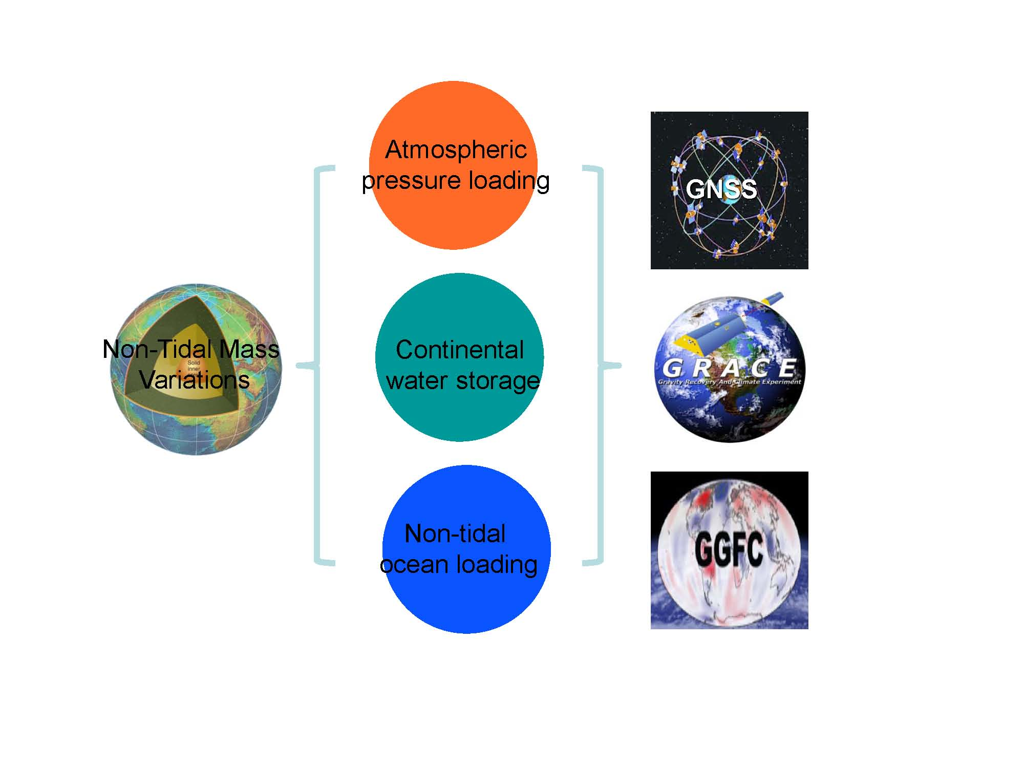
2.3. Surface Loading Datasets

Geophysical surface loading models are also widely used to estimate the non-tidal deformations and to correct seasonal variations in GNSS coordinate time series. In this paper, we computed vertical deformations from the Global Geophysical Fluid Center’s (GGFC) loading models [21]. The GGFC provides public access to calculate surface deformations driven by changes in ATML, CWS and NTOL with a spatial resolution of 2.5° × 2.5°. The GGFC ATML displacements need to be averaged into appropriate estimates corresponding to GNSS epochs from four daily solutions at the following epochs: 00, 06, 12, and 18. The GGFC CWS solutions are generated using the Noah-Version 1 GLDAS model and are provided in grids with monthly time interval. GLDAS soil moisture and the snow water equivalent were used in the inversions. The 3-dimensional deformations were derived using the method originally outlined in [46]. The twice-daily GGFC NTOL data were derived from the ocean bottom pressure (OBP) products with the Estimation of the Circulation and Climate of the Ocean (ECCO) Kalman Filter (kf080) series [47]. Moreover, as denoted by van Dam et al. (2001) and Jiang et al. (2014), long-term trends from NTOL data and CWS data were also removed before comparing them with GNSS results.

3. Results and Discussions

3.1. Consistency Analysis between GNSS, GRACE and GGFC

In this section, we interpret non-tidal deformations in vertical component of GNSS time series by comparing with the GRACE and GGFC derived VD series for the selected 186 stations. In our data analysis, CSR provides monthly GRACE SHC solutions since 2002, GGFC load models include atmospheric, non-tidal ocean and terrestrial water storage loading, and the GGFC NTOL and CWS data are available only for times before 2013. To eliminate the impacts of sampling rate differences and time span (temporal resolution), we unify the sampling rates (all data aiming to monthly solutions) and time span (2002/03-2012/12) of GNSS, GRACE, and GGFC solutions, and analyze the consistency among these datasets. Before correcting IG2 results with the corresponding results from GRACE and GGFC solutions, the IG2 GNSS time series are detrended.

3.1.1. Similarity of Annual Harmonic Signals

In order to get an overview of general properties of annually recurring signals for a larger number of stations, we follow the expression means of [25]. The amplitudes and phases of vertical annual signals estimated by GNSS, GRACE and GGFC observations are shown in Figure 2. The length of the vector represents the seasonal amplitude, and the vector direction points directly to the direction of the initial phase angles (counterclockwise from the beginning of the east).
Generally, at most stations, there are good consistency between GNSS, GGFC and GRACE. In terms of annual amplitudes, the range of GNSS amplitude is 0.3~10.5 mm. For the GRACE results, the annual amplitude range is 0.5~8.3 mm, and for the GGFC results, the annual amplitude range is 0.5~8.0 mm. The mean annual amplitude is 3.5 mm for GNSS, 2.7 mm for GRACE and 2.6mm for GGFC. Therefore, GNSS annual amplitudes are larger than those of both GRACE and GGFC, on average by a factor of about 1.3. Although GRACE and GGFC derived non-tidal deformations can interpret most of seasonal annual signals observed by GNSS, there are still annual amplitude variations remaining in the GNSS time series in addition to the surface deformation caused by hydrological, non-tidal ocean and atmospheric factors. For annual phases, differences between GNSS, GRACE and GGFC are small. The mean value of the annual phase difference for the GNSS versus (vs.) GRACE and GNSS vs. GGFC is 8.8° and 19.6°, indicating that there is no significant systematic phase difference between GNSS and GRACE data.
Figure 3 shows the harmonic annual VD estimated from GNSS monthly time series after removing the GRACE and GGFC modeled VD. Generally, seasonal amplitudes reduced with different levels for different stations. The amplitude of the GRACE correction result is larger than the GGFC correction result in the northern hemisphere, while the southern hemisphere is the opposite in most cases. The annual phase of GNSS-GRACE and GNSS-GGFC solutions is overall consistent, and the inconsistency mainly occurs in the Greenland region of the Northern Hemisphere and Central Europe.
Table 1 lists statistical results for annual signals from different techniques and combination solutions. On the whole, the annual amplitude of the GNSS time series is the most significant, followed by GRACE, and GGFC is the smallest, suggesting that in addition to the surface deformation caused by hydrological, non-tidal ocean and atmospheric factors, there are still annual amplitude variations remaining in the GNSS time series. After correcting the GNSS results with GRACE and GGFC loading deformations, the amplitude of the GNSS corrected by GGFC solutions is more optimal than the amplitude of the GNSS corrected by GRACE solutions, which may be owing to the filtering of the GRACE gravity field SHCs preprocessing. To some extent, this is to be expected, as the Gaussian averaging used to smooth the GRACE data also has the effect of reducing the amplitude of the true signal.

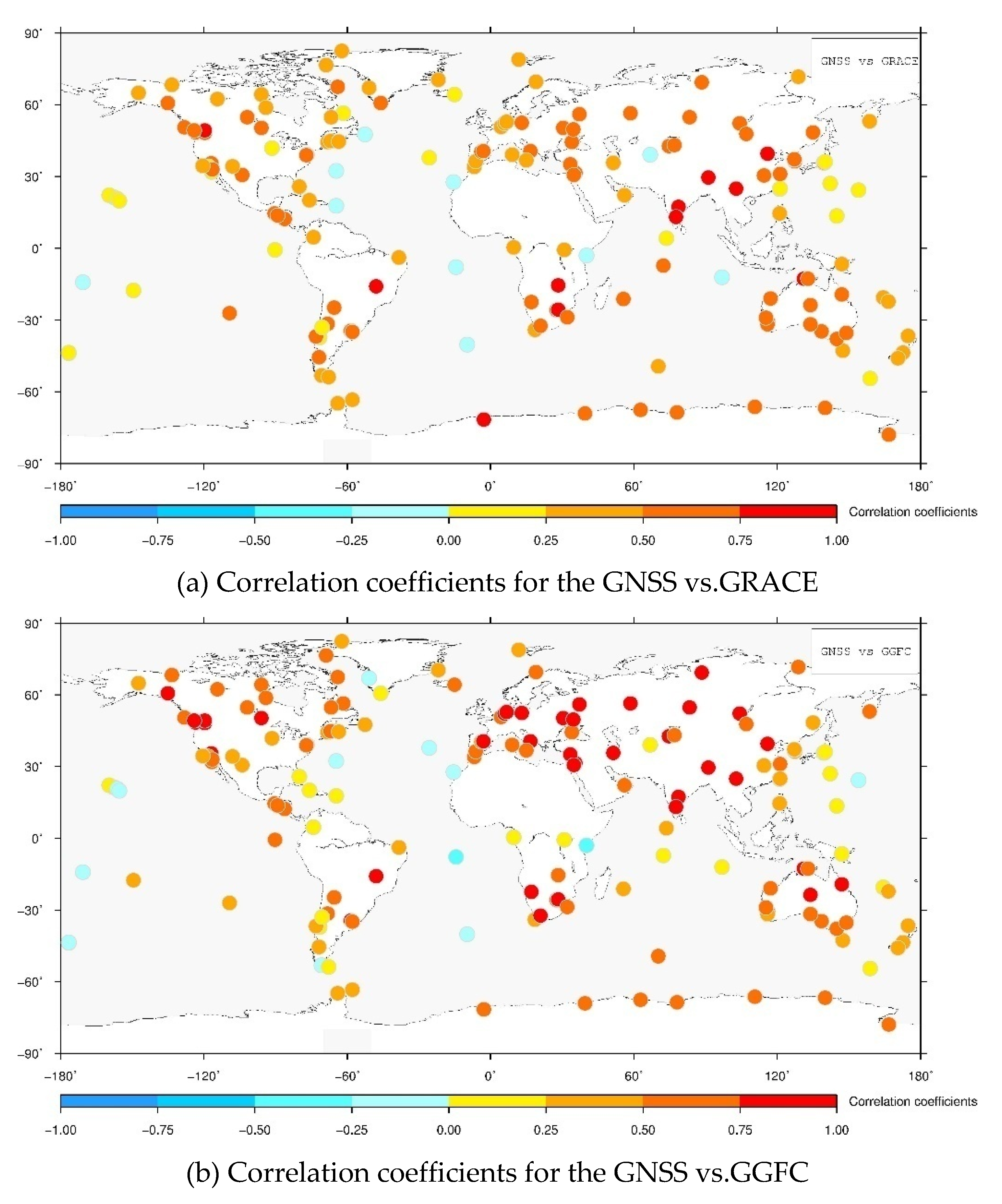
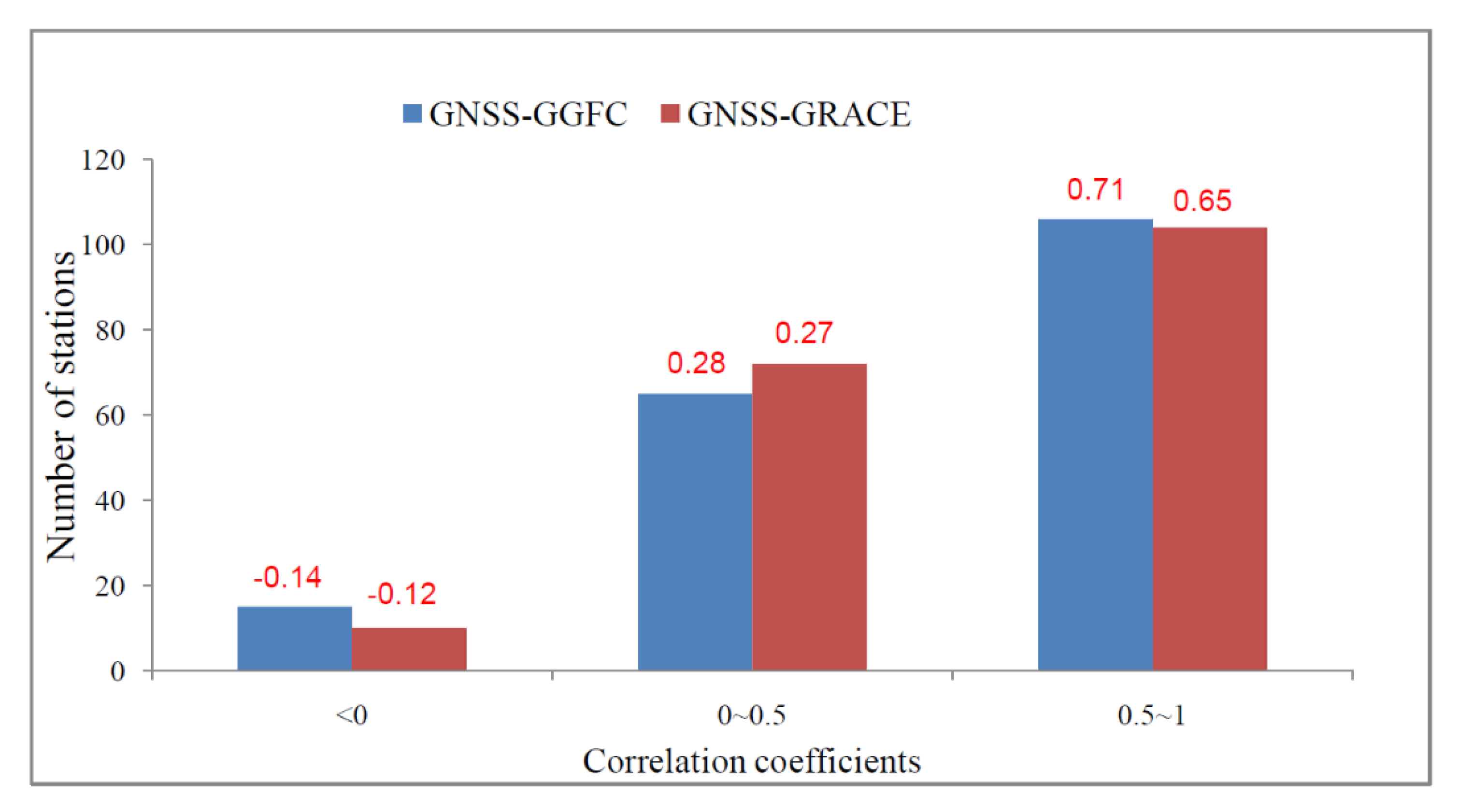
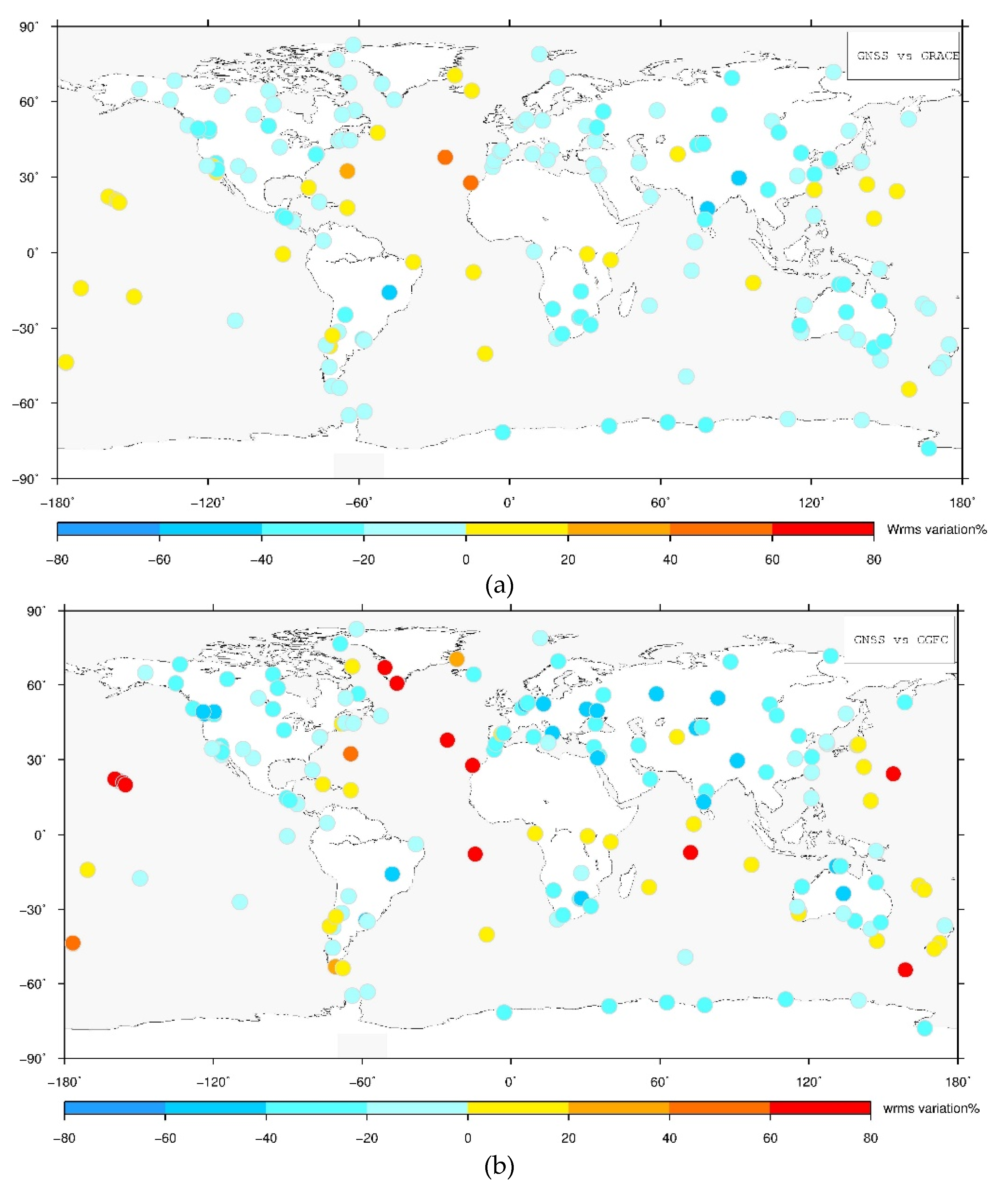
3.1.2. Quantitative Evaluation with Correlation Coefficient and WRMS Reduction

Figure 4 and Figure 5 display comparison results of the correlation coefficients of GNSS, GRACE and GGFC. Both results from GNSS vs. GRACE and GNSS vs. GGFC indicate a good correlation. Despite the number of stations with correlation larger than 0.5 between GNSS and GGFC being 2 more than that of between GNSS and GRACE, the number of stations with negative correlation for GNSS/GGFC is 5 more than that for GNSS/GRACE. The average of correlation coefficients is 0.45 and 0.49 for GNSS vs. GGFC and GNSS vs. GRACE, respectively, denoting that GRACE loading deformations are more consistent with GNSS series.
Accordingly, to further determine the similarity between GNSS, GRACE and GGFC VD series, the WRMS reduction of GNSS signal is illustrated by subtracting the GRACE or GGFC VD from the GNSS VD series. The W R M S reduction is calculated as 100 · ( W R M S G P S W R M S G P S G R A C E . or . G G F C W R M S G P S ) , where W R M S G P S is the signal W R M S of the GNSS data and W R M S G P S G R A C E . or . G G F C the signal W R M S of the GNSS corrected by GRACE solutions and GNSS corrected by GGFC solutions.
Figure 6 and Table 2 present the reduction in the GNSS signal W R M S by subtracting GRACE and GGFC deformations. The mean value of the W R M S variations for all 186 stations is −12.3% and −5.6%, respectively, for GNSS corrected by GRACE solutions and GNSS corrected by GGFC solutions. From Table 2, in terms of the station number, after correcting GNSS with GRACE and GGFC, there are 80% and 74% of stations displaying W R M S reduction. In terms of the W R M S reduction range, results for GGFC corrections have 24 more stations than that for GRACE for W R M S with 20% variations. For W R M S reduction between 0 and 20%, results for GRACE corrections have 35 more stations than that for GGFC corrections. For the correction effect of W R M S reduction more than 20%, the GNSS corrected by GGFC solutions are better than the GNSS with GRACE corrections in the number of stations (24 more stations). For the W R M S reduction interval of 0~20%, the GRACE correction effect is significantly better than the GGFC correction effect. The mean value of the W R M S reduction for the two types of correction results is close to each other, 33%/28% for reduction more than 20% and 10%/11% for reduction between 0 and 20%, respectively, for GNSS corrected by GGFC solutions and GNSS corrected by GRACE solutions. Nevertheless, for the 49 stations with W R M S increase in GNSS corrected by GGFC solutions, the average W R M S increase is 48%. Therefore, we conclude that the correction magnitude of GGFC loading is bigger than that of GRACE loading. However, the large magnitude is bidirectional, and the GGFC loading can bring better correction results for W R M S reduction more than 20%; at the same time, the amount of the W R M S increase is also larger than that of GRACE corrections. The GRACE corrections are generally better for the global stations and can be a more reliable choice when correcting the non-tidal loading deformations in GNSS stations around the world. This is mainly because the deficiency of the GGFC model in islands. For GGFC, ATML is modeled using input from the same NCEP surface pressure grids, NTOL is modeled using the same ECCO data as input, and CWS is modeled using the same GLDAS data soil moisture and snow water equivalent. For all data sets, the GGFC provides a Fortran program that uses a bi-cubic interpolation scheme that allows the user to interpolate the grids to any site. Both the original loading data and interpolation can introduce errors, especially for stations on ocean islands or small peninsulas where the physically expected loading signals are very small.

3.1.3. Sampling Effects on the Comparisons

To investigate the sampling effects on the conclusions, we re-do the comparison analysis based on the GGFC weekly solutions. Before illustrating the GGFC loading effects on GNSS coordinate time series, the combined GGFC solutions are re-sampled to GNSS weekly resolution solutions.
For the weekly solutions, the mean value of correlation coefficient is 0.44, and 48% of the stations have a correlation larger than 0.5, and only 7% of the stations have a negative correlation. After correcting the GNSS VD with GGFC solutions, 73% of the stations have their W R M S reduction, and 30% of the stations have a reduction larger than 20%. The statistical results are listed in Table 3. Comparison results indicate that the effects of the sampling rate of the data on the consistency of the GNSS and GGFC solutions are not significant in our analysis.

3.1.4. Remaining Disagreements between GNSS and GRACE or GGFC
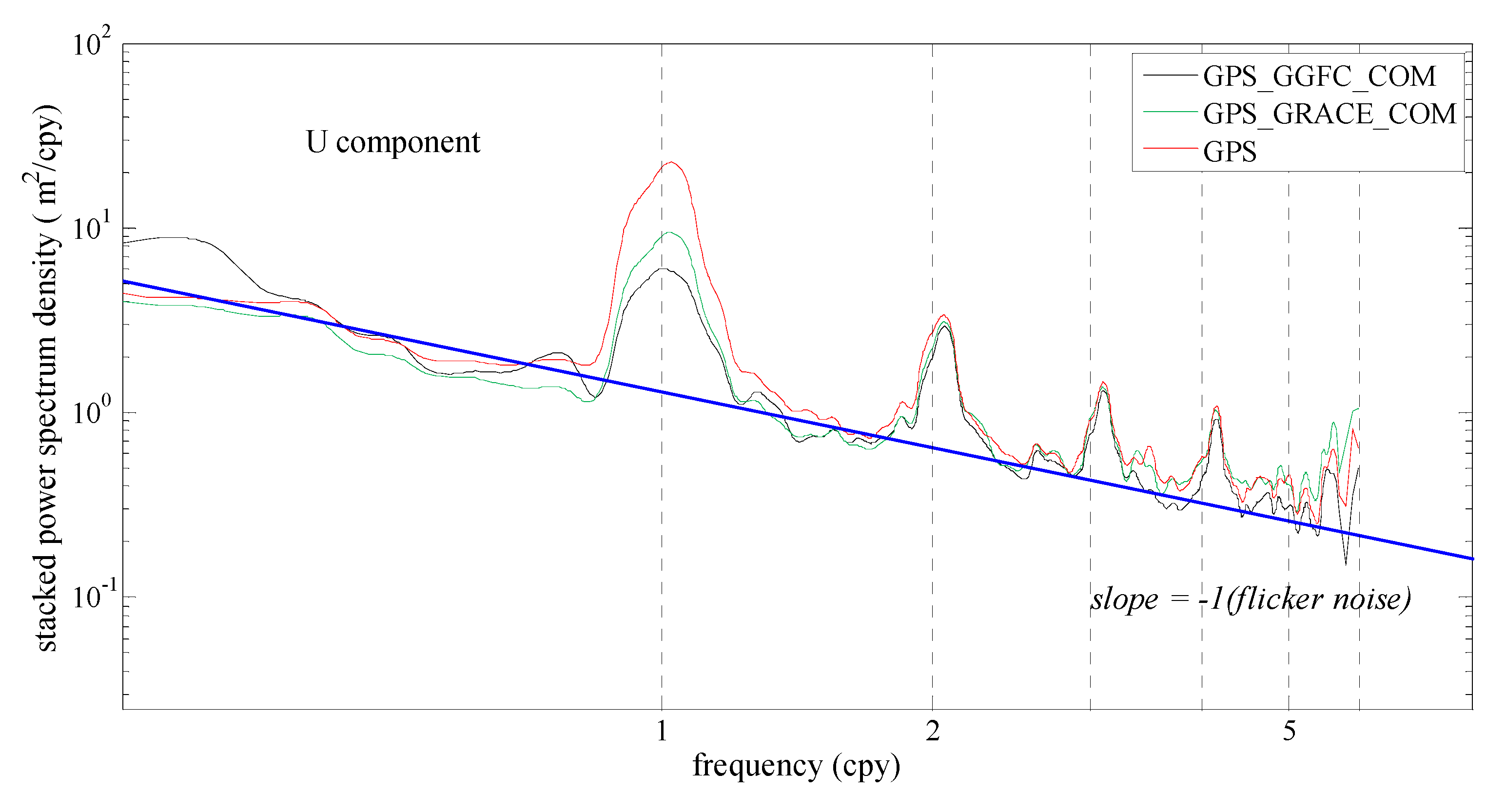
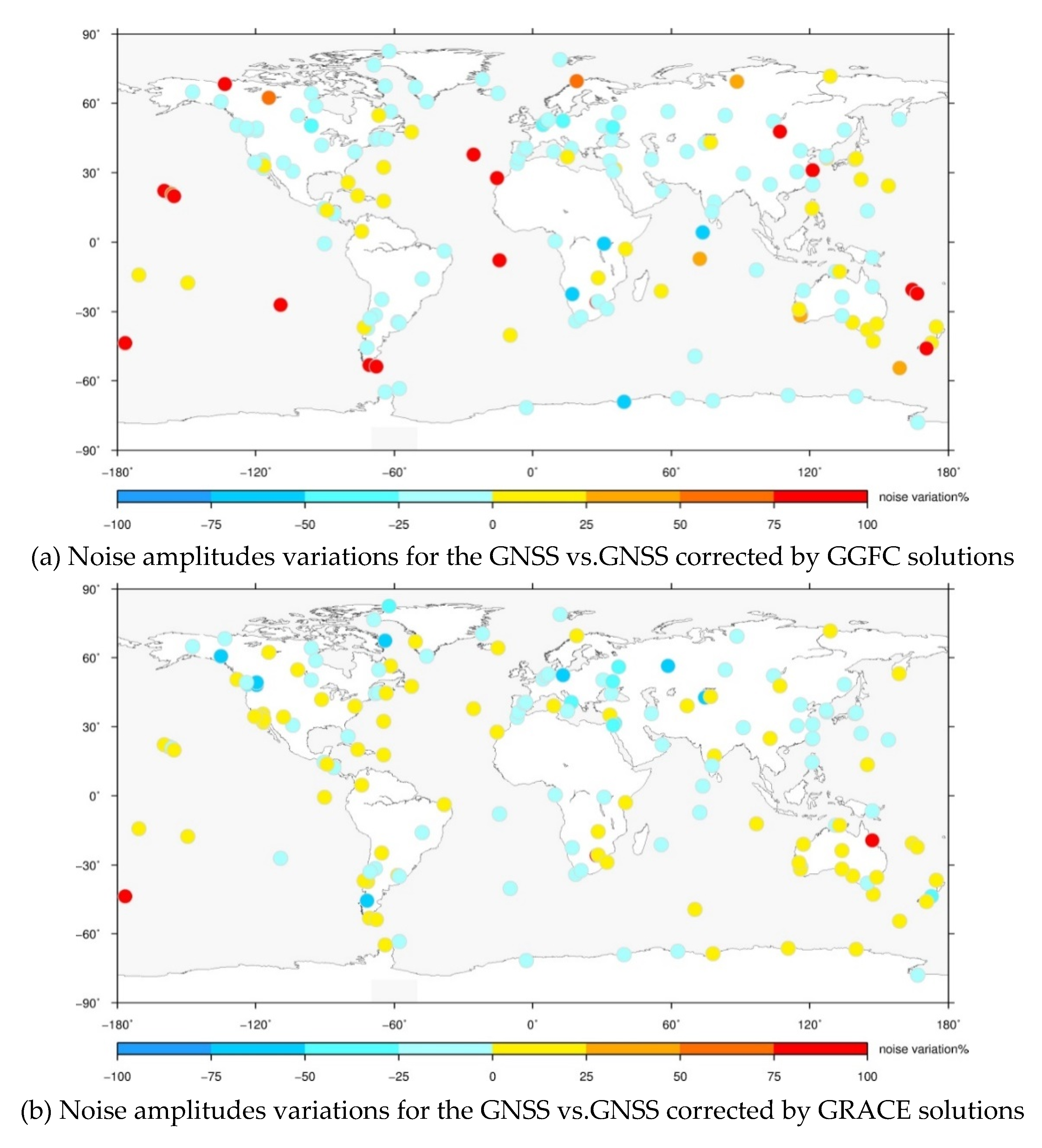
After subtracting GRACE or GGFC modeled non-tidal deformations from IG2solutions, seasonal signals still occur in the GNSS corrected by GRACE solutions and GNSS corrected by GGFC solutions, indicating the disagreement existing among the different techniques. There are two main error sources leading to the disagreement.
Firstly, there are shortcomings in the inversion process for both GRACE and GGFC models. The spatial resolutions, with about 300 km for GRACE and 2.5° grid for GGFC, denote that the two types of models have difficulties in distinguishing the surface mass loading appearing in small regional areas. The research of [20] demonstrated that the GRACE VDs from different institutes and different approaches are highly consistent. The incorporation of the degree 1 surface load coefficients from the GNSS deformations into GRACE computations can further improve comparisons. The GRACE follow-on plan also has great potential to correct the non-tidal loading in GNSS time series more effectively. For all GGFC datasets, ATML is modeled using input from the NCEP surface pressure grids, NTOL is modeled using the ECCO data as input, and CWS is modeled using the GLDAS data soil moisture and snow water equivalent. Both the original loading data and interpolation can introduce errors, especially for stations on ocean islands or small peninsulas where the physically expected loading signals are very small.
Secondly, GNSS signals not only contain the impacts of hydrology, non-tidal atmosphere, ocean tides, but also GNSS technique-related errors in data processing, such as processing noise effect, local multipath, and orbital errors. Previous researches have investigated the signals related to possible aspects in GNSS data processing, such as the draconitic errors caused by solar radiation pressure [34], satellite constellation and local multipath effects [33], unmodelled high frequency signals caused by S1 and S2 atmospheric pressure tides loading [48], subdaily EOP model, the effect of the thermal expansion of monuments and nearby bedrock [49]. The results indicate that the effect of these errors or mismodeling errors is related to seasonal signals in GNSS coordinate time series, but are not significant enough when comparing to the residuals between GNSS and GRACE/GMs data, and investigations on the ideal model for the effect of the mismodeling errors on GNSS data processing are still ongoing [48,49,50,51,52]. By the start of October 2019, the IGS ACs had begun the third reanalysis of the full history of GNSS data collected by the IGS global network since 1994 in a fully consistent way using the latest models and methodology.
However, it is difficult to provide the accurate/precise amplitudes of the above sources right now. In the following section, we do not try to declare the exact effects of the above options, but introduce one further aspect that reflects the total effect of the related errors, that is the noise in the coordinate time series [53,54,55]. GNSS measurements of position are temporally and spatially correlated rather than simply independent observations. The temporally correlated process for noise might characterize localized, random motions of the geodetic monument, the analysis errors in GNSS data processing, and the non-tidal loading effects. Therefore, we can adopt the noise characteristics as an indicator to decide which type of the non-tidal loading interpretation is better for the global IG2 coordinate time series.

3.2. Noise Analysis

In this part, we compute the power spectral density (PSD) of the three types of data—original GNSS solutions, GNSS corrected by GGFC solutions and GNSS corrected by GRACE solutions. The Lomb–Scargle periodogram method is applied to detect the noise characteristics in the log-log coordinate system [32,53,54]. In order to gain a global view of the PSD variations, all of estimated spectra are stacked by component and are smoothed with a Gaussian smoother using GMT software. Figure 7 shows the filtered PSD stacking results for the three types of solutions. The blue line with a slope of −1 denotes the power-law behavior of flicker noise in the log-log coordinate system. The overall noise behavior is similar for both IG2 solutions and the two types of IG2 combined solutions, and spectra of the flicker noise can describe the variations well for all three types of datasets. The noise characteristics become more and more white with the growing of the frequency. When the frequency expands higher than four cycles per year (cpy), a slope of 0 (white noise) could resemble the background noise well, either due to the intervention of a white noise frequency floor or because of a change in the basic characteristics of the underlying noise process to some type of non-integer power law intermediate between the flicker and white distributions [7,9,30].
The results also demonstrate that all three datasets have similar characteristics. The peaks are consistent for the three types of datasets, while the annual (1.0 cpy) is the most dominant frequency in all three datasets, and draconic signals are also obvious for the higher frequencies. However, the PSD amplitudes are different among the three datasets. After correcting GNSS solutions with GRACE- and GGFC-derived non-tidal mass variations, the stacked PSD amplitudes show an obvious decrease trend, especially for the annual frequency. This can be a useful clue to help us reduce some of seasonal signals in GNSS coordinate time series when reprocessing GNSS data corrected by GRACE or GGFC solutions.
We quantitatively analyze noise variations of the GRACE- and GGFC-derived non-tidal mass loadings on the global IGS stations. GNSS coordinate time series are assumed to consist of signal plus noise. To describe the signal, a trajectory model, which includes the linear trend, seasonal signals, offsets and post-seismic relaxation, is introduced [55]. The purpose of most GNSS time series analysis is to estimate accurately the parameters within the trajectory model. The residual which comes from subtracting the trajectory model from the observations represents the noise in GNSS time series.
To accurately compute noise characteristics of the GNSS time series, the optimal noise model needs to be defined first. Considering that different stations have different noise properties, many researchers have carefully investigated the appropriate noise models for different areas. Most recently, according to [55], for global stations, the preferred noise models are the power law (PL) or flicker noise (FN) with white noise (WN). Therefore, we select PL+WN and FN+WN, respectively, as the optimal noise model to describe the noise (residuals) existing in the above three types of data. The Create and Analyze Time Series (CATS) software is applied in the computations and the used trajectory model is a linear trend with an annual and semi-annual signal plus the aforementioned offsets.
Figure 8 displays total noise amplitudes (FN+WN) variations after correcting GNSS results with GGFC and GRACE solutions, respectively. For solutions with GGFC loading corrections, the number of stations with noise amplitudes decrease is 120/186, and the mean amplitude variations of stations with noise amplitude decrease and increase are 12.1% and 49.7%, respectively. The above three corresponding values for GNSS with GRACE corrections are 90/186, −12.5% and 10.5%. Although the GGFC loading can lead to more stations with noise decrease, noise amplitudes of stations with noise increase are much bigger than that of the solutions from GRACE corrections.
The average amplitudes of total amplitudes of the PL+WN for GNSS, GNSS-GGFC and GNSS-GRACE are 4.69, 4.92 and 4.46 mm, while for the FN+WN they are 4.61, 4.67 and 4.49 mm, respectively. The results indicate that for both types of optimal noise model, after subtracting the loading effects, GNSS corrected by GRACE solutions have the lowest noise level, demonstrating that the GNSS corrected by GRACE solutions present more favorable results than that of GNSS corrected by GGFC solutions. The GRACE deformations can occupy 5% of the noise behavior presenting in the global GNSS stations, while GGFC results could bring more than 5% of the noise into the global stations. Therefore, for the analysis of the surface loading effects on the global stations noise, GRACE can provide better results for these investigations.

3.3. Revisiting GRACE-Derived Non-Tidal DeformationWith GNSS Station PositionTime Series

The above analysis, especially the W R M S analysis and noise analysis, implies that GNSS corrected by GGFC solutions present a more stable and favorable results when explaining the non-tidal mass variations remaining in the IG2coordinate time series. In the following sections, we further evaluate the consistency between GNSS-observed and GRACE-modeled vertical deformations to help us to better interpret the differences between the two geodetic techniques.

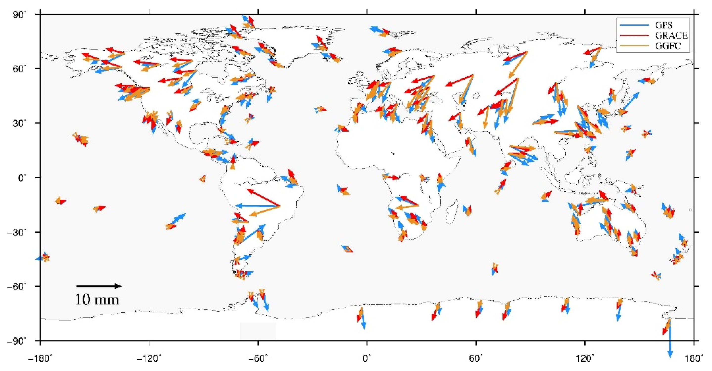
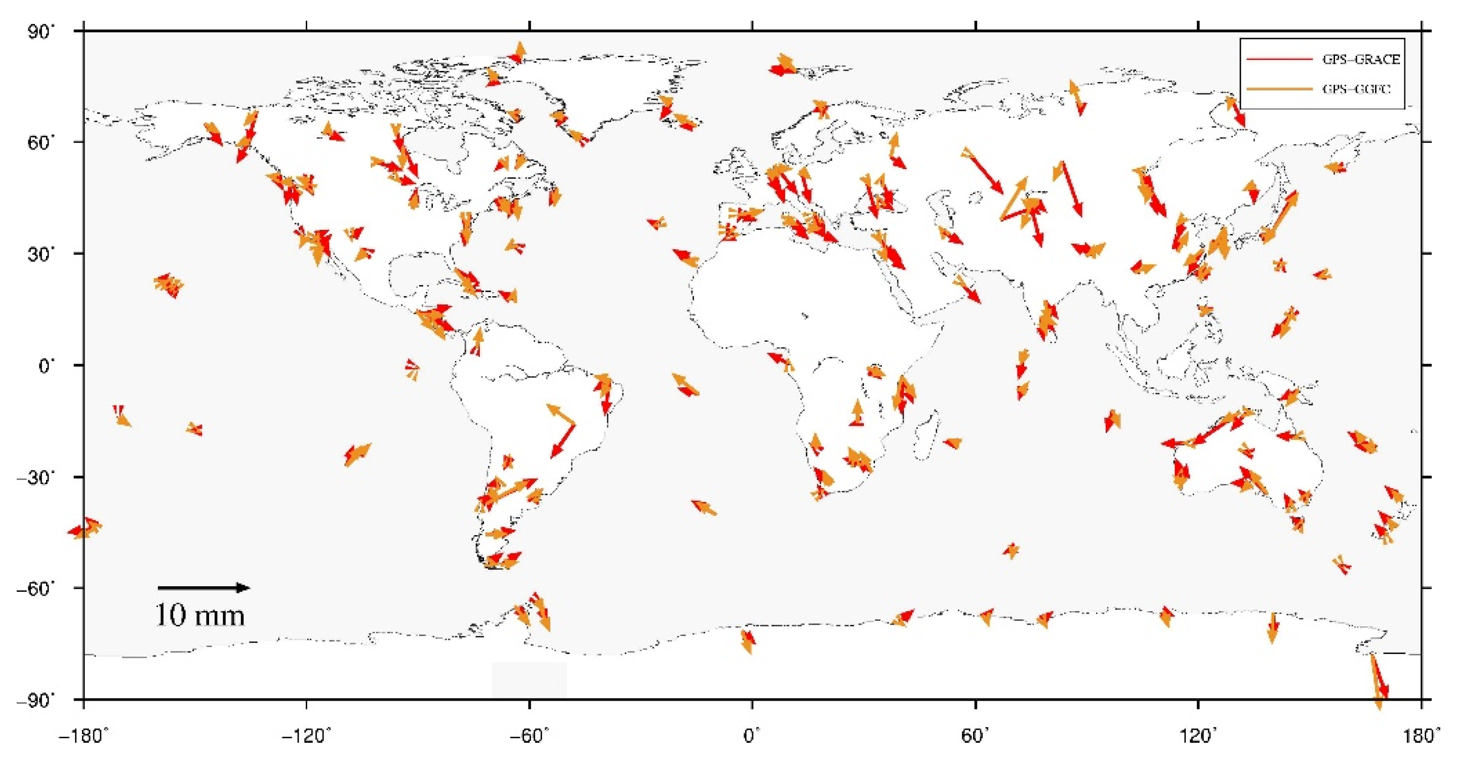
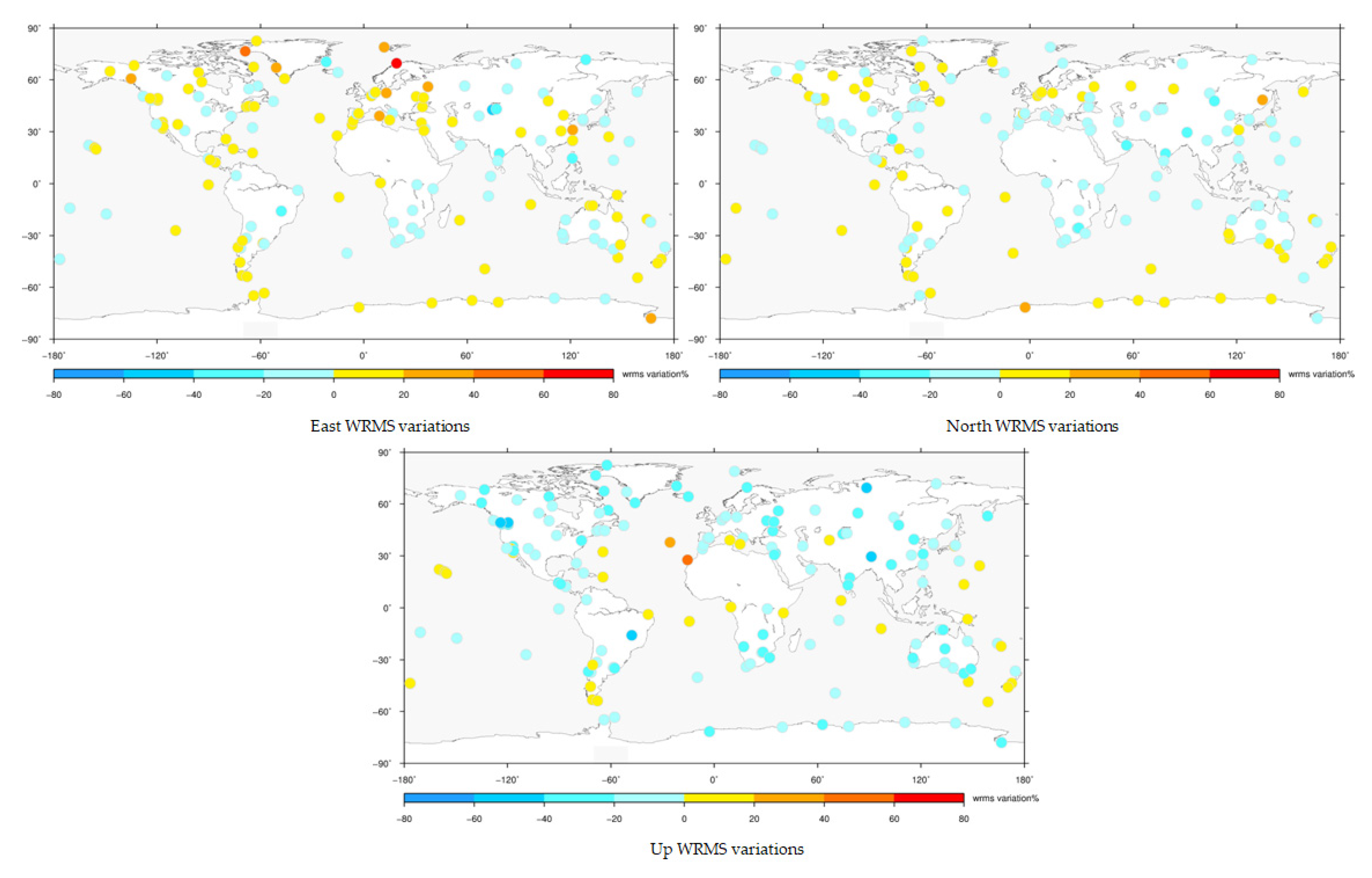
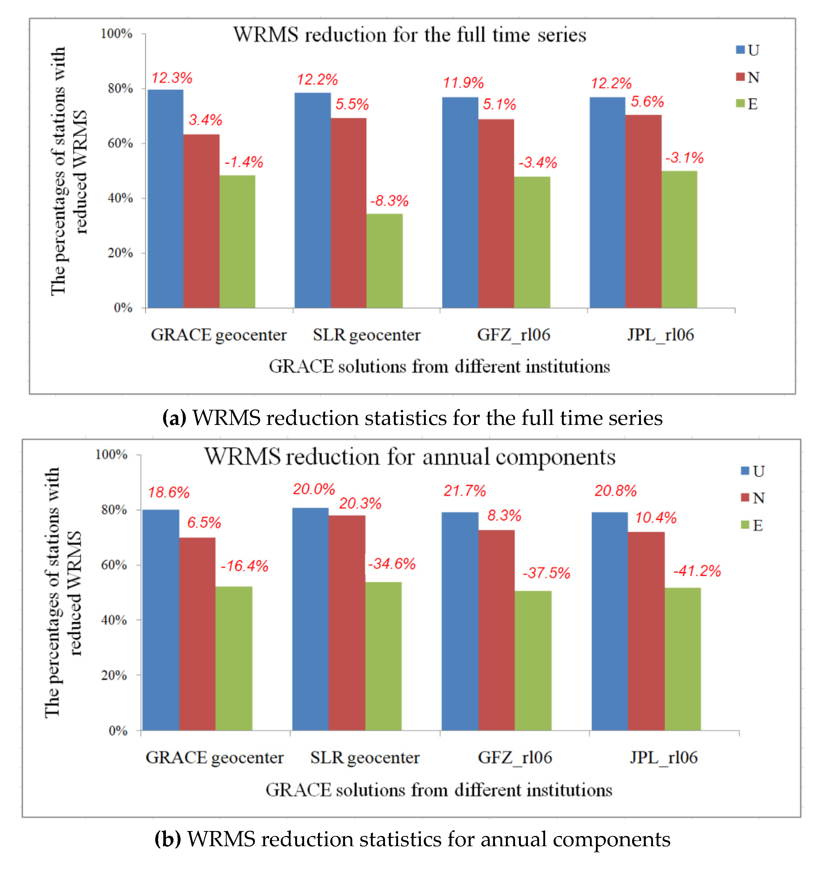
3.3.1. Horizontal Deformations Variations

Firstly, we compare the IG2 horizontal time series with GRACE-derived horizontal deformations to address the relations for the horizontal deformations. Figure 9 displays W R M S reductions for the east, north, and vertical components, respectively (red depicts a reduction larger than 20%, yellow between 0 and 20% reduction, and blue if signal W R M S is added). The results indicate significant disagreement with the horizontal deformations at the global scale, especially for the east component (the noticeable blue arrow), while for the vertical component, the IG2 displacement is fairly well predicted by GRACE solutions. Figure 10 states mean W R M S values and percentages of stations at which the W R M S is reduced when correcting the deformations with GRACE solutions, which can further confirm the discrepancy between the vertical and horizontal predictions of observed GNSS signals [13]. A common argument to explain this discrepancy is the spatial resolution of GRACE, a larger part of horizontal deformations being attributed to high spherical harmonics degree loads—that is, short wavelength loads—that GRACE cannot resolve [12,56]. GRACE-modeled non-tidal loadings from multiple institutions (GeoForschungs Zentrum/Potsdam, Germany (GFZ) and Jet Propulsion Laboratory (JPL)) are also compared with the IG2 solutions. The W R M S variations are listed in Figure 10. An overall consistency among the solutions from the different GRACE institutions is displayed.

3.3.2. Degree-1 SHC Effects on the GNSS/GRACE Results

The degree-1 SHC in the Earth’s gravity field (geocenter motion) cannot be observed with satellite-to-satellite tracking. Although GNSS receivers on each GRACE spacecraft do give some sensitivity to their position relative to the Earth’s surface, the sensitivity is not yet strong enough to give good degree-1 solutions [26]. Thus, the degree-1 SHC are not provided accurately in GRACE solutions. In the above section, we adopted the degree-1 time series provided by research of [44] to inverse the surface deformations. Here, we add the degree-1SHCs obtained from the analysis of SLR data into the GRACE solutions and perform the same processing and analyzing program as with the above section. The W R M S reductions are also listed in Figure 10. The results indicate that the difference between SLR geocenter SHCs and the research of [44] geocenter SHCs is not obvious for the W R M S variations of the vertical component. Meanwhile, for the horizontal components, only for the east component, the GRACE solutions corrected with SLR geocenter perform less favorably.

4. Discussions

4.1. Comparison to Previous Work

In the research of [25], almost 80% of the 115 GNSS stations had their W R M S decreased after subtracting GRACE from GNSS time series, while our analysis shows that GNSS signal W R M S decreases at almost 80% of the 186 stations, indicating that we have 56 more stations presenting the expected improvements. Both the results from [25] and our analysis show that nearly 6% of the stations have a negative correlation, and the mean correlation coefficient is 0.48 and 0.49 for [25] and our results, respectively. With regard to the results of [26], our W R M S reduction indicates reasonable results (mean W R M S reductionis12% for both). Although the percentages of these parameters are close to each other, our analysis is based on 186 stations, which is 62% more than the 115 stations of [25] and 69% more than the 110 stations of [26]. All of these factors can confirm the reliability of the analysis.
Moreover, we select results from [28] to probe the improvements of IG2 solutions relative to IG1 solutions. The research of [28] found about 64% of the 233 stations to have W R M S decrease after subtracting vertical deformations from the GGFC loading model; our analysis demonstrates that 74% of the 186 stations have a W R M S reduction. For the number of stations with W R M S decrease greater than 10%, [28] found 26% of these stations to have a W R M S decrease greater than 10%, while our analysis indicates that 53% of all the stations have GNSS signal W R M S decrease. We found 37 more stations as having W R M S decrease than that of [28]. Overall, we can find that our analysis with GNSS/GGFC solutions is more optimal than that of [28], and better results can be noted than previous research comparing GNSS with GGFC loading models. All improvements should be ascribed to the improvements from IG1 to IG2 solutions.

4.2. Thermal ExpansionEffects

Except for the VD induced by the non-tidal loading effects, the observed GNSS height changes are also influenced by thermal expansion. With respect to GNSS solutions, the GRACE mission and GGFC solutions can only capture the signals caused by mass variations, and the effects of thermal expansion of monuments and nearby bedrock did not appear in the GRACE and GGFCVD data [12,57]. To investigate the thermo-elastic effect on GNSS, the research of [57] extended a theoretical model to estimate the thermal expansions of GNSS monuments and nearby bedrock for 86 globally distributed GNSS stations based upon measurements of surface air temperatures. Their results show that annual temperature variations are the dominant contributors for the thermal expansion of GNSS monuments and nearby bedrock. The contributions of thermal expansion to GNSS height changes display largely spatial variations and can reach to 3.9 mm, which is significantly larger than the prediction from [12]. While the research of [58] indicated that the predicted amplitude of the thermally induced surface deformation in the global scale is at the millimeter level with the largest ∼2 mm. More recently, the research of [20] also used the annual amplitudes and phases from [57] to correct the effect of the thermal expansion of monuments and nearby bedrock. In their research, only four solutions among eleven solutions showed an improvement after thermal expansion correction, suggesting that the effect of thermal expansion is not significant in the residuals between GNSS and GRACE data, due to the large uncertainty in the GNSS postprocessing methods. Therefore, the thermal effects due to local thermal variations on GNSS observations still need to be carefully taken into account in an analysis of seasonal geophysical signals.

4.3. Leakage ErrorsAnalysis

All water storage observations from GRACE represent average values, in both space and time. Temporally, GRACE data are approximately monthly averaged quantities. Because of truncation and filtering in the spectral domain, GRACE data are also spatially averaged, with spatially varying weights [59]. This results in a time series that differs from the true, i.e., uniformly weighted, time series; this difference is often referred to as ‘‘leakage’’. The leakage error depends on the filtering process as well as the characteristics of the signal [59,60]. The truncation of GRACE SHCs and needed spatial filtering and smoothing to suppress the longitudinal stripping noises will introduce leakage bias and degrade the spatial resolution of GRACE-determined surface mass variations [59]. In order to reduce this leakage error, the research of [59] derived gain factors (basin-scale gain factors and grid-point gain factors) by minimizing the misfit between the unfiltered, true, and filtered GRACE water storage time series through a simple least square regression.
Right now, the methods handling the leakage error effects are mainly based on region (basin) scale and are mostly used in the regional water storage analysis. For the leakage errors at one point, we try to correct the GRACE leakage error by adding the corrections derived from the Global Land Data Assimilation System (GLDAS) Noah outputs (transformed into SHC with degree and order up to 60) by calculating the differences between the original GLDAS modeled VD and the truncated and filtered GLDAS VD at each IG2 station. However, the differences between GLDAS filtered and unfiltered solutions display largely temporal variations and can reach up to tens of centimeters, which is far larger than the non-tidal loadings effects. Meanwhile, the comparison results between GNSS and GRACE derived solutions with these leakage errors corrections are far from satisfactory. Moreover, the research of [20] investigated the leakage error effects by comparing the GRACE SHC solutions and the most recently released GRACE mass concentration (MASCON) solutions which have been confirmed to have a high resolution and fewer leakage errors. However, all the indicators considered in their study show that the GRACE MASCON and SHC solutions have a similar ability to interpret the GNSS signals, suggesting that the VD signals are insusceptible to the smoothing. Mean annual amplitude reduction of the 11 GNSS-Observed VD solutions corrected with CSR SHC modeled solutions and with CSR MASCON modeled solutions are both 0.32 [20]. The conclusions of the leakage errors effects on the comparisons between GNSS and GRACE are equally valid for this study.

5. Conclusions

In this paper, we compare the seasonal VD time series derived from IG2, GRACE and GM solutions for 186 globally distributed IGS core stations over global region. We provide a thorough evaluation of the potential of two totally independent solutions to observe the non-tidal loading signal in GNSS, and also attempt to explain the remaining GNSS–GRACE/GM residuals. Our analysis can provide users with more clues to decide which model is better for their research when analyzing the seasonal signals over the global stations. The most meaningful analysis include two points: (1) we provide a thorough evaluation of the potential of two totally independent solutions (GRACE and GM) to observe the non-tidal loading signal in GNSS and (2) we investigate the noise properties of the GNSS corrected by GRACE solutions and GNSS corrected by GGFC solutions for global stations using optimal noise models.
The results demonstrate the intrinsic relationship between GNSS and GRACE or GGFC vertical deformation mentioned above. After correcting the GNSS results with GRACE and GGFC loading deformations, the amplitude of the GNSS corrected by GGFC solutions is more optimal than the amplitude of the GNSS corrected by GRACE solutions, which may be owing to the filtering of the GRACE gravity field spherical harmonic coefficient preprocessing. The average of the correlation coefficients is 0.45 and 0.49 for GNSS vs. GGFC and GNSS vs. GRACE, respectively, indicating that GRACE loading deformations are more consistent with GNSS series. The mean value of the W R M S variations for all 186 stations is −12.3% and −5.6%, respectively, for GNSS vs. GRACE and GNSS vs. GGFC solutions. The GRACE correction improvement is generally better for the global stations and can be a more reliable choice when correcting the environmental loading deformation in GNSS stations around the world.
Moreover, we introduce one further aspect that reflects the total effect of the related errors, namely the noise in the coordinate time series. Through the noise analysis with the optimal noise models, we can find that after subtracting the loading effects from the IG2 coordinate time series, the GNSS/GRACE solutions have the lowest noise level, demonstrating that the GNSS-GRACE combination solutions present more favorable results than that of GNSS-GGFC solutions. The GRACE deformations can occupy 5% of the noise behavior presenting in the global GNSS stations, while the GGFC results could bring more than 5% of the noise into the global stations.
Finally, we revisit GRACE-derived loading deformation with GNSS station position time series in terms of the horizontal deformations, degree-1 coefficients effects and solutions from different institutions, and also try to perform comparisons with the previous research and detail the thermal expansion effects and leakage errors analysis. Our results display an improvement over the analyses presented by previous works, which may owe to the development of the GNSS data processing. Therefore, for the analysis of the surface loading effects on the global stations noise, the GRACE can provide better results for these research.

Author Contributions

Conceptualization, L.D. and H.C.; Methodology, L.D., Q.C.; Software, L.D.; Validation, L.D., and Q.C.; Formal analysis, A.M., H.C.; Investigation, L.D.; Resources, A.M., H.C.; Data curation, L.D.; Writing—original draft preparation, L.D., H.C.; Visualization, A.M.; Funding acquisition, H.C. All authors have read and agreed to the published version of the manuscript.

Funding

This research was funded by the National Science Fund for Distinguished Young Scholars of China (Grant No. 41525014), the National Natural Science Foundation of China (NO. 41974019, 41704030), the Scientific Research Project of Hubei Provincial Department of Education (No. Q20194501), the Surveying and Mapping Basic Research Program of National Administration of Surveying, Mapping and Geoinformation (No.17-01-01) and Research Program of Hubei Polytechnic University (No.18xjz09R).

Acknowledgments

We thank IGS for providing IG2products, CSR/GFZ/JPL for providing GRACE solutions and GGFC for providing the GM series.

Conflicts of Interest

The authors declare no conflict of interest.

References

  1. Altamimi, Z.; Rebischung, P.; Métivier, L.; Collilieux, X. ITRF2014: A new release of the International Terrestrial Reference Frame modeling nonlinear station motions. J. Geophys. Res. 2016, 121, 6109–6131. [Google Scholar] [CrossRef] [Green Version]
  2. Jin, S.; Van Dam, T.; Wdowinski, S. Observing and understanding the earth system variations from space geodesy. J. Geodyn. 2013, 72, 1–10. [Google Scholar] [CrossRef] [Green Version]
  3. Van Dam, T.; Wahr, J.; Chao, Y.; Leuliette, E. Predictions of crustal deformation and of geoid and sea-level variability caused by oceanic and atmospheric loading. Geophys. J. Int. 1997, 129, 507–517. [Google Scholar]
  4. Klos, A.; Gruszczynska, M.; Bos, M.S.; Boy, J.P.; Bogusz, J. Estimates of vertical velocity errors for IGS ITRF2014 stations by applying the improved singular spectrum analysis method and environmental loading models. Pure Appl. Geophys. 2018, 175, 1823–1840. [Google Scholar] [CrossRef]
  5. Bogusz, J.; Klos, A. On the significance of periodic signals in noise analysis of GPS station coordinates time series. GPS Solut. 2016, 20, 655–664. [Google Scholar] [CrossRef] [Green Version]
  6. Collilieux, X.; Van Dam, T.; Ray, J.; Coulot, D.; Métivier, L.; Altamimi, Z. Strategies to mitigate aliasing of loading signals while estimating GPS frame parameters. J. Geod. 2012, 86, 1–14. [Google Scholar] [CrossRef]
  7. Ray, J.; Altamimi, Z.; Collilieux, X.; Van Dam, T. Anomalous harmonics in the spectra of GPS position estimates. GPS Solut. 2008, 12, 55–64. [Google Scholar] [CrossRef]
  8. Amiri-Simkooei, A.R.; Mohammadloo, T.H.; Argus, D.F. Multivariate analysis of GPS position time series of JPL second reprocessing campaign. J. Geod. 2017, 91, 685–704. [Google Scholar] [CrossRef] [Green Version]
  9. Jiang, W.; Deng, L.; Li, Z.; Zhou, X.; Liu, H. Effects on noise properties of GPS time series caused by higher-order ionospheric corrections. Adv. Space Res. 2014, 53, 1035–1046. [Google Scholar] [CrossRef]
  10. Penna, N.T.; Stewart, M.P. Aliased tidal signatures in continuous GPS height time series. Geophys. Res. Lett. 2003, 30, 2184–2188. [Google Scholar] [CrossRef] [Green Version]
  11. Rebischung, P.; Altamimi, Z.; Ray, J.; Garayt, B. The IGS contribution to ITRF2014. J. Geod. 2016, 90, 611–630. [Google Scholar] [CrossRef]
  12. Dong, D.; Fang, P.; Bock, Y.; Cheng, M.K.; Miyazaki, S. Anatomy of apparent seasonal variations from GPS-derived site position time series. J. Geophys. Res. 2002, 107, ETG-9. [Google Scholar] [CrossRef] [Green Version]
  13. Chanard, K.; Fleitout, L.; Calais, E.; Rebischung, P.; Avouac, J.P. Toward a global horizontal and vertical elastic load deformation model derived from GRACE and GNSS station position time series. J. Geophys. Res. 2018, 123, 3225–3237. [Google Scholar] [CrossRef]
  14. Han, S.C. Elastic deformation of the Australian continent induced by seasonal water cycles and the 2010–2011 La Niña determined using GPS and GRACE. Geophys. Res. Lett. 2017, 44, 2763–2772. [Google Scholar] [CrossRef]
  15. Mannel, B.; Dobslaw, H.; Dill, R.; Glaser, S.; Balidakis, K.; Thomas, M.; Schuh, H. Correcting surface loading at the observation level: Impact on global GNSS and VLBI station networks. J. Geod. 2019, 93, 2003–2017. [Google Scholar] [CrossRef]
  16. Roggenbuck, O.; Thaller, D.; Engelhardt, G.; Franke, S.; Dach, R.; Steigenberger, P. Loading-Induced Deformation Due to Atmosphere, Ocean and Hydrology: Model Comparisons and the Impact on Global SLR, VLBI and GNSS Solutions. In International Association of Geodesy Symposia; REFAG, 2014; Van Dam, T., Ed.; Springer: Cham, Switzerland, 2015; Volume 146. [Google Scholar]
  17. Nordman, M.; Virtanen, H.; Nyberg, S.; Mäkinen, J. Non-tidal loading by the Baltic Sea: Comparison of modeled deformation with GNSS time series. GeoResJ 2015, 7, 14–21. [Google Scholar] [CrossRef] [Green Version]
  18. Davis, J.L.; Elosegui, P.; Mitrovica, J.X.; Tamisea, M.E. Climate-driven deformation of the solid earth from GRACE and GPS. Geophys. Res. Lett. 2004, 31, L24605. [Google Scholar] [CrossRef] [Green Version]
  19. Fu, Y.; Freymueller, J. Seasonal and long-term vertical deformation in the Nepal Himalaya constrained by GPS and GRACE measurements. J. Geophys. Res. 2012, 117, B3. [Google Scholar] [CrossRef]
  20. Gu, Y.; Yuan, L.; Fan, D.; You, W.; Su, Y. Seasonal crustal vertical deformation induced by environmental mass loading in mainland China derived from GPS, GRACE and surface loading models. Adv. Space Res. 2017, 59, 88–102. [Google Scholar] [CrossRef]
  21. Van Dam, T.; Altamimi, Z.; Collilieux, X.; Ray, J. Topographically induced height errors in predicted atmospheric loading effects. J. Geophys. Res. 2010, 115, 307–309. [Google Scholar] [CrossRef]
  22. Van Dam, T.; Wahr, J.; Milly, P.C.D.; Shmakin, A.B.; Blewitt, G.; Lavallée, D.; Larson, K.M. Crustal displacements due to continental water loading. Geophys. Res. Lett. 2001, 28, 651–654. [Google Scholar] [CrossRef] [Green Version]
  23. Yan, H.; Chen, W.; Yuan, L. Crustal vertical deformation response to different spatial scales of GRACE and GCMs surface loading. Geophys. J. Int. 2016, 204, 505–516. [Google Scholar] [CrossRef] [Green Version]
  24. Liu, R.; Zou, R.; Li, J.; Zhang, C.; Zhao, B.; Zhang, Y. Vertical Displacements Driven by Groundwater Storage Changes in the North China Plain Detected by GPS Observations. Remote Sens. 2018, 10, 259. [Google Scholar] [CrossRef] [Green Version]
  25. Tesmer, V.; Steigenberger, P.; van Dam, T.; Mayer-Gürr, T. Vertical deformations from homogeneously processed GRACE and global GPS long-term series. J. Geod. 2011, 85, 291–310. [Google Scholar] [CrossRef]
  26. Gu, Y.; Fan, D.; You, W. Comparison of observed and modeled seasonal crustal vertical displacements derived from multi-institution GPS and GRACE solutions. Geophys. Res. Lett. 2017, 44, 7219–7227. [Google Scholar] [CrossRef]
  27. Rothacher, M.; Angermann, D.; Artz, T.; Bosch, W.; Drewes, H.; Gerstl, M.; Kelm, R.; König, D.; König, R.; Meisel, B.; et al. GGOS-D: Homogeneous reprocessing and rigorous combination of space geodetic observations. J. Geod. 2011, 85, 679–705. [Google Scholar] [CrossRef]
  28. Jiang, W.; Li, Z.; Van Dam, T.; Ding, W. Comparative analysis of different environmental loading methods and their impacts on the GPS height time series. J. Geod. 2014, 87, 687–703. [Google Scholar] [CrossRef]
  29. Van Dam, T.; Wahr, J.; Lavallée, D. A comparison of annual vertical crustal displacements from GPS and Gravity Recovery and Climate Experiment (GRACE) over Europe. J. Geophys. Res. 2007, 112, B03404. [Google Scholar] [CrossRef] [Green Version]
  30. Zhu, Z.; Zhou, X.; Deng, L.; Wang, K.; Zhou, B. Quantitative analysis of geophysical sources of common mode component in CMONOC GPS coordinate time series. Adv. Space Res. 2017, 60, 2896–2909. [Google Scholar] [CrossRef]
  31. Williams, S.D.P.; Penna, N.T. Non-tidal ocean loading effects on geodetic GPS heights. Geophys. Res. Lett. 2011, 38, L09314. [Google Scholar] [CrossRef] [Green Version]
  32. Deng, L.; Jiang, W.; Li, Z.; Chen, H.; Wang, K.; Ma, Y. Assessment of second- and third-order ionospheric effects on regional networks: Case study in china with longer CMONOC GPS coordinate time series. J. Geod. 2016, 91, 1–21. [Google Scholar] [CrossRef]
  33. King, M.A.; Watson, C.S. Long GPS coordinate time series: Multipath and geometry effects. J. Geophys. Res. 2010, 115, B04403. [Google Scholar] [CrossRef]
  34. Rodriguez-Solano, C.J.; Hugentobler, U.; Steigenberger, P.; Lutz, S. Impact of Earth radiation pressure on GPS position estimates. J. Geod. 2012, 86, 309–317. [Google Scholar] [CrossRef] [Green Version]
  35. Deng, L.; Li, Z.; Wei, N.; Ma, Y.; Chen, H. GPS-derived geocenter motion from the IGS second reprocessing campaign. Earth Planets Space 2019, 71, 74. [Google Scholar] [CrossRef]
  36. Völksen, C. Reprocessing of a regional GPS network in Europe. In Observing Our Changing Earth: Proceedings of the 2007 IAG General Assembly, Perugia, Italy, 2–13 July 2007; Sideris, M.G., Ed.; Springer Science & Business Media: Berlin, Germany; New York, NY, USA, 2008; pp. 57–64. [Google Scholar]
  37. Maciuk, K. The Study of Seasonal Changes of Permanent Stations Coordinates based on Weekly EPN Solutions. Artif. Satell. 2016, 51, 1–18. [Google Scholar] [CrossRef] [Green Version]
  38. Dousa, J.; Vaclavovic, P.; Elias, M. Tropospheric products of the second GOP European GNSS reprocessing (1996–2014). Atmos. Meas. Tech. 2017, 10, 3589–3607. [Google Scholar] [CrossRef] [Green Version]
  39. Tapley, B.D.; Bettadpur, S.; Watkins, M.; Reigber, C. The gravity recovery and climate experiment: Mission overview and early results. Geophys. Res. Lett. 2004, 31, L09607. [Google Scholar] [CrossRef] [Green Version]
  40. Kusche, J.; Schrama, E. Surface mass redistribution inversion from global GPS deformation and Gravity Recovery and Climate Experiment (GRACE) gravity data. J. Geophys. Res. 2005, 110. [Google Scholar] [CrossRef] [Green Version]
  41. Bettadpur, S. UTCSR Level-2 Processing Standards Document for Product Release 0006; GRACE 327-742; Center for Space Research, The University of Texas at Austin: Austin, TX, USA, 2018. [Google Scholar]
  42. Chen, J.L.; Wilson, C.R.; Tapley, B.D.; Grand, S. GRACE detects coseismic and postseismic deformation from the Sumatra-Andaman earthquake. Geophys. Res. Lett. 2007, 34. [Google Scholar] [CrossRef] [Green Version]
  43. Swenson, S.; Wahr, J. Post-processing removal of correlated errors in GRACE data. Geophys. Res. Lett. 2006, 33, L08402. [Google Scholar] [CrossRef]
  44. Sun, Y.; Riva, R.; Ditmar, P. Optimizing estimates of annual variations and trends in geocenter motion and J2 from a combination of GRACE data and geophysical models. J. Geophys. Res. 2016, 121, 8352–8370. [Google Scholar] [CrossRef] [Green Version]
  45. Flechtner, F. GRACE AOD1B Product Description Document (Rev. 2.1); GRACE 327-750 (GR-GFZ-AOD-0001); GeoForschungsZentrum Potsdam: Potsdam, Germany, 2005. [Google Scholar]
  46. Van Dam, T.; Wahr, J. Displacements of the Earth’s surface due to atmospheric loading: Effects on Gravity and Baseline Measurements. J. Geophys. Res. 1987, 92, 1281–1286. [Google Scholar] [CrossRef]
  47. Kim, S.B.; Lee, T.; Fukumori, I. Mechanisms controlling the interannual variation of mixed layer temperature averaged over the Nio-3 region. J. Clim. 2007, 20, 3822–3843. [Google Scholar] [CrossRef]
  48. Tregoning, P.; Watson, C. Atmospheric effects and spurious signals in GPS analyses. J. Geophys. Res. 2009, 114, B09403. [Google Scholar] [CrossRef] [Green Version]
  49. Xu, X.; Dong, D.; Fang, M.; Zhou, Y.; Wei, N.; Zhou, F. Contributions of thermoelastic deformation to seasonal variations in GPS station position. GPS Solut. 2017, 21, 1265–1274. [Google Scholar] [CrossRef]
  50. Chew, C.C.; Small, E.E. Terrestrial water storage response to the 2012 drought estimated from the vertical position anomalies. Geophys. Res. Lett. 2014, 41, 6145–6151. [Google Scholar] [CrossRef]
  51. Han, S.C. Seasonal clockwise gyration and tilt of the Australian continent chasing the center of mass of the Earth’s system from GPS and GRACE. J. Geophys. Res. 2016, 121, 7666–7680. [Google Scholar] [CrossRef]
  52. Zou, R.; Freymueller, J.T.; Ding, K.; Yang, S.; Wang, Q. Evaluating seasonal loading models and their impact on global and regional reference frame alignment. J. Geophys. Res. 2014, 119, 1337–1358. [Google Scholar] [CrossRef]
  53. Williams, S.D.P. The effect of coloured noise on the uncertainties of rates estimated from geodetic time series. J. Geod. 2003, 76, 483–494. [Google Scholar] [CrossRef]
  54. Langbein, J. Estimating rate uncertainty with maximum likelihood: Differences between power-law and flicker-random-walk models. J. Geod. 2012, 86, 775–783. [Google Scholar] [CrossRef] [Green Version]
  55. He, X.; Bos, M.S.; Montillet, J.P.; Fernandes, R.M.S. Investigation of the noise properties at low frequencies in long GNSS time series. J. Geod. 2019, 93, 1271–1282. [Google Scholar] [CrossRef]
  56. Fu, Y.; Argus, D.F.; Freymueller, J.T.; Heflin, M.B. Horizontal motion in elastic response to seasonal loading of rain water in the Amazon Basin and monsoon water in Southeast Asia observed by GPS and inferred from GRACE. Geophys. Res. Lett. 2013, 40, 6048–6053. [Google Scholar] [CrossRef]
  57. Yan, H.; Chen, W.; Zhu, Y.; Zhang, W.; Zhong, M. Contributions of thermal expansion of monuments and nearby bedrock to observed GPS height changes. Geophys. Res. Lett. 2009, 36. [Google Scholar] [CrossRef] [Green Version]
  58. Fand, M.; Dong, D.; Hager, B.H. Displacements due to surface temperature variation on a uniform elastic sphere with its centre of mass stationary. Geophys. J. Int. 2014, 196, 194–203. [Google Scholar]
  59. Landerer, F.; Swenson, S.C. Accuracy of scaled GRACE terrestrial water storage estimates. Water Resour. Res. 2012, 48. [Google Scholar] [CrossRef]
  60. Wiese, D.N.; Landerer, F.; Watkins, M.M. Quantifying and reducing leakage errors in the JPL RL05M GRACE mascon solution. Water Resour. Res. 2016, 52, 7490–7502. [Google Scholar] [CrossRef]
Figure 1. Spatial distribution of the selected 186 global navigation satellite system (GNSS) stations.
Remotesensing 12 02477 g001
Figure 2. Harmonic annual vertical deformation (VD) derived from GNSS (blue), Gravity Recovery and Climate Experiment (GRACE) (red) and Global Geophysical Fluid Center (GGFC) (yellow) for monthly time series. The length of the vector represents the seasonal amplitude, and the vector direction points directly to the direction of the initial phase angles.
Remotesensing 12 02477 g002
Figure 3. Harmonic annual VD derived from GNSS monthly time series after removing the GRACE (red) and GGFC (yellow) modeled VD. The length of the vector represents the seasonal amplitude, and the vector direction points directly to the direction of the initial phase angles.
Remotesensing 12 02477 g003
Figure 4. Correlation coefficients for the GNSS vs. GRACE (upper panel) and GNSS vs. GGFC (bottom panel) time series.
Remotesensing 12 02477 g004
Figure 5. Histogram of statistical results for the correlation coefficients (the red text above the histogram represents the average of the correlation coefficients).
Remotesensing 12 02477 g005
Figure 6. Weighted root mean square (WRMS) reduction ratio by correcting GNSS VDs with loading from GRACE (upper panel) (a) and GGFC (bottom panel) (b).
Remotesensing 12 02477 g006
Figure 7. Stacked periodogram of the coordinate time series. The black vertical lines represent the 1.0 cycle per year (cpy) harmonics, respectively. The power-law behavior of flicker noise is denoted by the blue line with a slope of −1.
Remotesensing 12 02477 g007
Figure 8. Noise amplitudes variations for the GNSS vs.GNSS corrected by GGFC solutions (up panel) and GNSS vs. GNSS corrected by GRACE solutions (bottom panel) solutions.
Remotesensing 12 02477 g008
Figure 9. WRMS reductions obtained for the east, north and vertical components using GRACE-derived deformations corrections.
Remotesensing 12 02477 g009
Figure 10. WRMS reduction statistics from the comparison of the IG2 time series and GRACE deformations (the red text above the histogram represents the average of WRMS reduction).
Remotesensing 12 02477 g010
Table 1. Annual signals statistical results for the monthly time series.
Data TypeAnnual Amplitudes (mm)Annual Phase (°)
GNSS3.5196.2
GGFC2.6176.6
GRACE2.7187.4
GNSS corrected by GGFC1.7192.9
GNSS corrected by GRACE2.2207.6
Table 2. Statistical results for the WRMS reduction.
Data Types WRMS% > 0WRMS% < 0−20% < WRMS% < 0WRMS% < −20%
GNSS corrected by GGFCNumber of stations491375285
Mean value of WRMS47.6%−24.6%−10.2%−33.4%
GNSS corrected by GRACENumber of stations381488761
Mean value of WRMS9.7%−17.9%−10.8%−28.1%
Table 3. Statistical results of the GNSS and GGFC with different sampling rates.
IndexMonthly SolutionsWeekly Solutions
Annual amplitudes and phases2.6 mm/176.9°2.6 mm/167.5°
Stations with WRMS reduction74%73%
Mean values of WRMS variations−5.6%−5.4%
Correlation coefficients0.450.44

