Internal Waves at the UK Continental Shelf: Automatic Mapping Using the ENVISAT ASAR Sensor

Abstract

Oceanic internal waves occur within stratified water along the boundary between water layers of different density and are generated when strong tidal currents flow over seabed topography. Their amplitude can exceed 50 m and they transport energy over long distances and cause vertical mixing when the waves break. This study presents the first fully automated methodology for the mapping of internal waves using satellite synthetic aperture radar (SAR) data and applies this to explore their spatial and temporal distribution within UK shelf seas. The new algorithm includes enhanced edge detection and spatial processing to target the appearance of these features on satellite images. We acquired and processed over 7000 ENVISAT ASAR scenes covering the UK continental shelf between 2006 and 2012, to automatically generate detailed maps of internal waves. Monthly and annual internal wave climatology maps of the continental shelf were produced showing spatial and temporal variability, which can be used to predict where internal waves have the most impact on the seabed environment and ecology in UK shelf seas. These observations revealed correlations between the temporal patterns of internal waves and the seasons when the continental shelf waters were more stratified. The maps were validated using well-known seabed topographic features. Concentrations of internal waves were automatically identified at Wyville-Thomson Ridge in June 2008, at the continental shelf break to the east of Rosemary Bank in January 2010 and in the Faroe-Shetland Channel in June 2011. This new automated methodology has been shown to be robust for mapping internal waves using a large SAR dataset and is recommended for studies in other regions worldwide and for SAR data acquired by other sensors.

1. Introduction

Oceanic internal waves (IWs) usually develop in stratified water, in which pycnoclines form boundaries that separate water layers of different density. The density difference may be driven by temperature (thermoclines) or salinity (haloclines), with thermoclines occurring more commonly in the open ocean. IWs are common in continental shelf regions, and where brackish water overlies saltwater at the mouths of large rivers. IWs can be generated by strong tidal currents that flow over a seabed of varying topography, such as shelf breaks and shallow sills. IWs are responsible for transferring energy between the large-scale tides and small-scale mixing. On the continental shelf, when their energy reaches the seabed, the shear stress causes sediment disturbance and resuspension. Areas prone to such disturbance form an ideal habitat for certain benthic animals, and hence should be considered for protection when planning offshore developments such as renewable energy devices and oil and gas platforms.

A deeper understanding of the mechanisms of IW formation and interaction with the coastal environment requires the collection and analysis of large volumes of experimental measurements. Traditionally, measurements of IW fields have been carried out using instruments deployed in the ocean, such as moored buoys equipped with temperature, salinity and ocean current sensors or by using acoustic instruments such as sonars on ships. However, in situ measurements are time-consuming, expensive and unsuitable for large-scale observations. Remote sensing (RS) methods provide an alternative to in situ observations of IWs. RS methods are inexpensive and can provide excellent spatial coverage and consistency of observations. They provide insight into the space-time distribution of IWs that are dynamic and diverse.

Synthetic Aperture Radar (SAR) sensors have demonstrated excellent capability for observation of IWs from space. SAR sensors operate by detecting the return of a pulse of radiation in the microwave band and are insensitive to cloud cover and solar illumination. Hence, they can provide all-weather, day and night monitoring of IWs on the ocean surface. Their operation principles are based on high sensitivity to small-scale roughness of the ocean surface induced by wind. The manifestation of IWs in SAR images can be seen as bright and dark bands. Two mechanisms are involved in the generation of intensity bands: modulation of the surface roughness by surface current associated with IWs; and damping of the surface capillary waves by oils and films that tend to concentrate in the regions of surface water convergence, where they form slicks.

Rapid growth in the volume of data produced by satellite SAR sensors over the last decade has stimulated the development of new methods for automatic analysis of SAR images. Several approaches have been developed in the literature for the detection of IWs in SAR data. Rodenas and Garello [1] used a 2-D spectral analysis based on short-time Fourier transform (STFT) to study IW packets in ERS-1 SAR images and to estimate packet wavelength. A similar technique was applied by Changbao et al. [2] to evaluate the dominant wavelength and propagation direction. Rodenas and Garello [3] suggested that the wavelet transform (WT) can perform better than STFT in locating irregularities of the IW signal. They used an analytical IW model to develop a set of wavelet basis functions that were adapted to the IW signatures and applied these functions for analysis of IW patterns in ERS-1 SAR images of the Strait of Gibraltar. The approach based on WT was further extended and a fully automatic tool was developed for detection and orientation estimation of IWs in the ERS-1 SAR images in [3]. The tool employed decomposition of SAR images into different scales using 2-D dyadic WT to suppress speckle noise and improve the accuracy of edge detection. The output of the multi-resolution edge detector was further processed to discriminate look-alike features such as ship wakes, oil slicks and currents. Rodenas and Garello [3] demonstrated the efficiency of this method by processing individual ERS-1 and RADARSAT SAR scenes.

A multiple-stage methodology for IW detection using stationary wavelet transform (SWT) was proposed by Simonin et al. [4], including pre-processing, edge extraction and edge analysis stages. To discriminate look-alikes from the IW features, Simonin et al. [4] implemented an analysis of geometric features of IW edges. However, the algorithm was tested on a very limited set of images and a more detailed study was needed to select IW detection parameters and optimise its performance in various conditions. Bao et al. [5] suggested a convolutional neural network approach for automatic detection of IWs in SAR images produced by the ENVISAT Advanced Synthetic Aperture Radar (ASAR) sensor. The neural network was trained using a database of 950 scenes of IWs in the South China Sea region. The system demonstrated overall good performance but incorrectly identified river estuaries and coastline features [5].

Hence, several advanced approaches have been developed for automatic detection of IWs in satellite images, but none of these have yet been applied to routine processing of large datasets and automatic generation of IW maps. In contrast, a number of SAR studies of the geographical distribution of IWs were based on manual/visual analysis of satellite images. Dokken et al. [6] studied IW activity along the coast of Norway using more than 2600 ERS and RADARSAT-1 images, though the IWs were not combined as a map. Zhao et al. [7] published maps showing the distribution of 116 IW crests in the South China Sea manually traced on ERS-1/2 and Envisat SAR data. Lorenzetti and Dias [8] identified over 460 IW packets in the southeastern continental shelf of Brazil using visual analysis of 264 Envisat SAR images. Kozlov et al. [9] used SAR data to map spatial statistics of short-period IWs in the Kara Sea, based on 89 ENVISAT ASAR images acquired between July and October 2007.

Many studies use a multi-sensor approach for investigation of IWs from space [10,11,12,13,14], based on the joint use of SAR and optical sensor data. Lavrova and Kostianoy [10] processed and analysed SAR and multispectral sensor images to study the temporal and spatial variability of IWs in the Caspian Sea. Several years of Envisat ASAR, Sentinel-1A,1B SAR, Sentinel-2 MSI and Landsat-8 OLI scenes were processed to build a composite map of IW packets to investigate their behaviour with changes in sea surface temperature. Zhou et al. [11] built annual, seasonal and monthly distribution maps of IWs in the Andaman Sea by combining MODIS Terra/Aqua optical and Sentinel-1 SAR images. The SAR sensor was mainly used to fill the gaps in optical data during complex weather conditions. Ning et al. [12] applied data acquired by Sentinel-1 SAR and Gaofen-3 SAR sensors in different periods of time to extend the interval of IW observations in the Malacca Strait. The SAR images were analysed manually to estimate the amplitude and group velocity of IWs. These parameters were linked to the seabed topography in the Malacca Strait. Mitnik et al. [13] applied SAR images acquired by Envisat ASAR, Sentinel-1 and ALOS PALSAR satellite sensors at various polarisations to study IWs and other mesoscale dynamic features generated by the Oyashio current in the northwestern Pacific Ocean. Satellite visible and infrared images were used to complement SAR data. Observations of IWs in the Flores Sea, Indonesia were studied using the Himawari-8 geostationary satellite optical sensor, in combination with MODIS optical sensor images and Sentinel-1 SAR images [14]. Our literature review did not discover any previous studies of the distribution of IWs on the UKCS using satellite data, but studies have been carried out in other parts of the world, where internal waves are frequently observed [6,9,11,12,14].

The review of published literature shows that the study of the geographical distribution and other characteristics of IWs can benefit from the joint processing of satellite data acquired by multiple sensors. Satellite images of IWs were mainly processed manually to minimise detection errors, but this approach also leads to large processing time that only increases with the application of different sensors. In this paper, we attempt to solve this problem by implementing a fully automatic approach that eliminates human errors and enables the processing of large volumes of satellite images. By applying statistical techniques to estimate the geographical distribution of IWs, we reduced the impact of image noise and detection errors. We approach the problem of IW detection in SAR images by considering it as an edge detection task. The problem of edge detection has been extensively studied in the fields of image processing and computer vision [15]. The Canny edge detection algorithm is one of the most successful, providing good accuracy, efficiency and simplicity. We adopted this algorithm for the detection of IW features in SAR data. Based on the Canny algorithm, we have developed a methodology for automatic processing of ENVISAT advanced synthetic aperture radar (ASAR) sensor data and applied this methodology to investigate internal waves on the UK continental shelf (UKCS) in 2006–2012. For this time period, we produced maps of internal wave distribution and climatology. Through this novel approach, we aim to realise the full value of existing and future satellite SAR datasets for systematic observational studies of these important physical oceanographic features.

2. Study Region and Datasets

2.1. Study Region

The study was carried out for most of the UKCS, including Dogger Bank in the North Sea, the extension of the UKCS region west of Rockall and parts of the Faroe-Shetland Channel. The continental slope in these areas plays an important role in bringing nutrients to the region and supporting a wide diversity of marine species [16,17]. The outline of the UKCS region used in this study is shown in red in Figure 1, which also shows the bathymetry and seabed topographical features.

2.2. ENVISAT ASAR Data

IWs were detected on the UKCS by processing the archive of ASAR sensor data acquired in 2006–2012 by the ENVISAT mission and accessed through the ESA EO Data Gateway Service (https://eogrid.esrin.esa.int/). Data were acquired using both vertical (VV) and horizontal (HH) co-polarisation. However, only VV polarisation data were applied to IW detection due to higher sensitivity to variations in sea surface roughness [19].

The ASAR sensor can operate using one of five image acquisition modes, of which the wide swath (WS) mode is most appropriate for IW detection in the UKCS as it achieves the best combination of spatial resolution and coverage. In WS mode the sensor swath is 405 km and the spatial resolution of each pixel is about 150 m × 150 m with a 50% overlap, so the pixel spacing is about 75 m × 75 m. These characteristics are sufficient to acquire more than 1000 images of the UKCS each year and detect most IW features in the area. We examined the total number of ASAR overpasses that were available each month in the sample year 2009. The number of overpasses ranged from 51 in December to 109 in March (see

Table 1. Number of overpasses overlapping the entire region of interest in each month of 2009.

Month	Number of Overpasses
January	83
February	78
March	109
April	69
May	85
June	70
July	64
August	85
September	83
October	79
November	52
December	51

). There are several reasons why the number of overpasses varied each month: changes of sensor observation timetable and modes; sensor failures and degradation of data quality for some overpasses. The average number of possible overpasses was determined by satellite orbit and the latitude that affects sensor track spacing. The density of the Earth’s surface observations is significantly greater for higher latitudes. For the ENVISAT ASAR sensor, the frequency of revisiting the same location at latitude 60° with incidence angle >5° is six times per 35 days or every 5.8 days [20].

The ENVISAT ASAR overpasses acquired in WS mode and overlapping with the UKCS in Figure 1 were downloaded and stored for further processing. The results of the preliminary analysis of selected SAR scenes are shown in Figure 2, where the revisit time averaged over the years 2006–2012 was plotted against the month number. It is seen in Figure 2 that a sufficient number of observations is available in the UKCS: on average, any given location was observed every 6.5 days (5.4 times in 35 days) and the maximum interval between observations was 7.9 days in April. The climatology data also show a slight variation in the number of available images in different months (maximum 16% deviation from the mean).

Figure 3 shows the spatial distribution of the revisit time values averaged over the years 2006–2012. It can be seen that sensor data cover the entire UKCS area. The revisit time depends on the location, varying from 20 days in the most distant parts to the west to 3.3 days in the north-east of the North Sea.

Overall, this analysis demonstrates that the number of available ENVISAT ASAR sensor measurements can be sufficient for the estimation of IW monthly, seasonal and annual frequency maps.

3. Methods

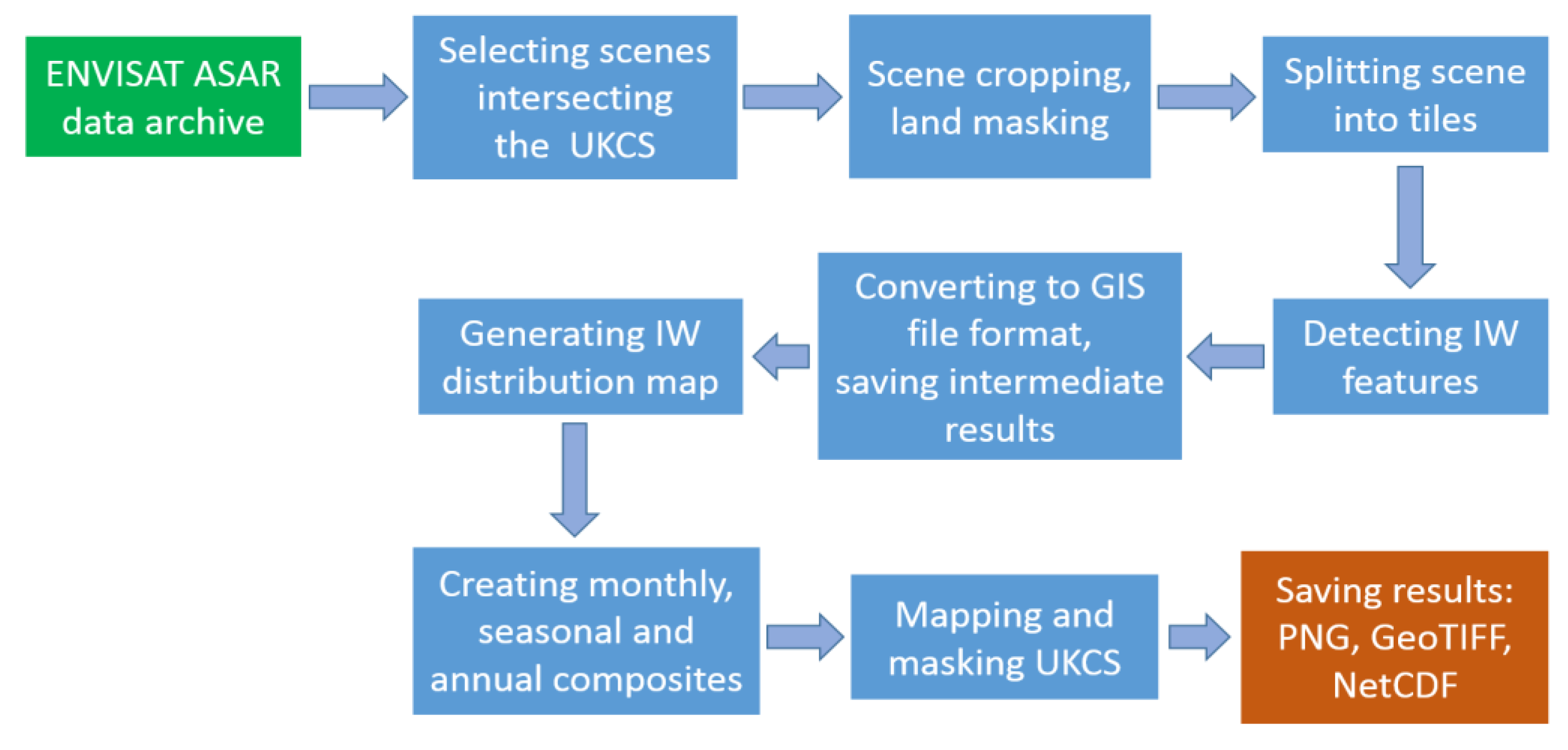
3.1. Data Processing Chain

The multistage and fully functional processing chain has been developed for automatic processing of the archive of ENVISAT ASAR images. The processing chain is shown in the block diagram in Figure 4 with the arrows indicating the data flow. The chain is implemented using the Python programming language and uses the Sentinel Application Platform (SNAP), the ESA open-source platform for Earth observation processing and analysis.

At the first data processing stage, the ASAR archive was scanned to select overpasses that geographically overlap with the UKCS outlined in Figure 1. Each of the selected scenes was then processed as follows. First, the image was cropped to include only a section that overlaps with the UKCS. This helps to reduce the size of the processed image and minimise computational expenses. The cropped image was then masked to exclude land from further processing. The land mask was generated using the SRTM3 Shuttle Radar Topography Mission terrain elevation data, with 3 arc seconds spatial resolution in good agreement with that of the ASAR images.

Each ENVISAT ASAR dataset consists of many millions of pixels, hence tiling is necessary. We selected a tile size of 2000 × 2000 pixels. There may be three or more tiles along the swath, depending on how much of the orbit intersects the UKCS.

The next stage in the block diagram in Figure 4 was to extract the contours of IWs in the image, then apply tests to discriminate true IW features from non-IW edges. This was applied to the original level 1 ASAR data to avoid any loss of data due to image resampling and mapping. The intermediate results of IW detection were saved in the PNG image format at native ASAR resolution. The results of IW detection were applied at the next processing stage to produce the IW occurrence maps that show the frequency of IW observation for different regions of the UKCS (Section 4). Any data outside the UKCS were masked out and the images were mapped into the geographic Lat/Lon projection, WGS 84 geographic datum. Maps with pixel size 10 × 10 arc minutes, or 19 km in latitude and 10 km in longitude at UK latitudes, were generated and saved in PNG, GeoTIFF and NetCDF data format. The stages in the processing chain are detailed in the following sections.

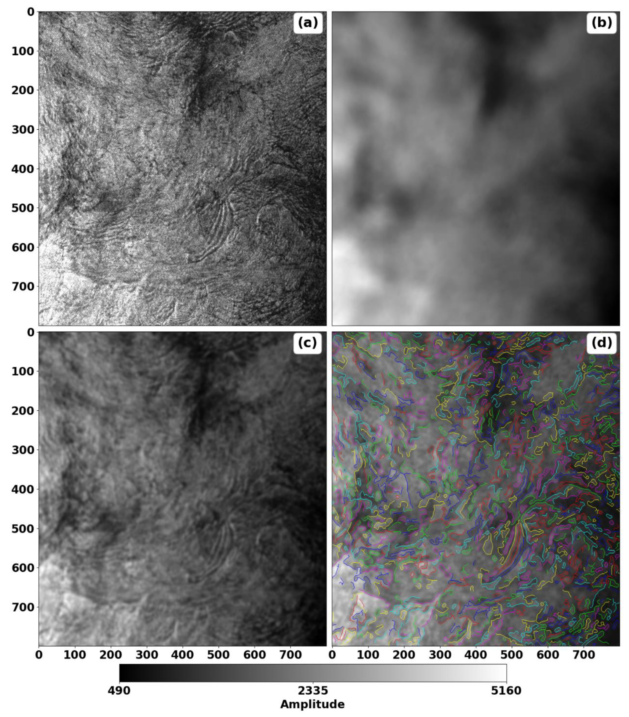
3.2. Automatic Detection of IWs

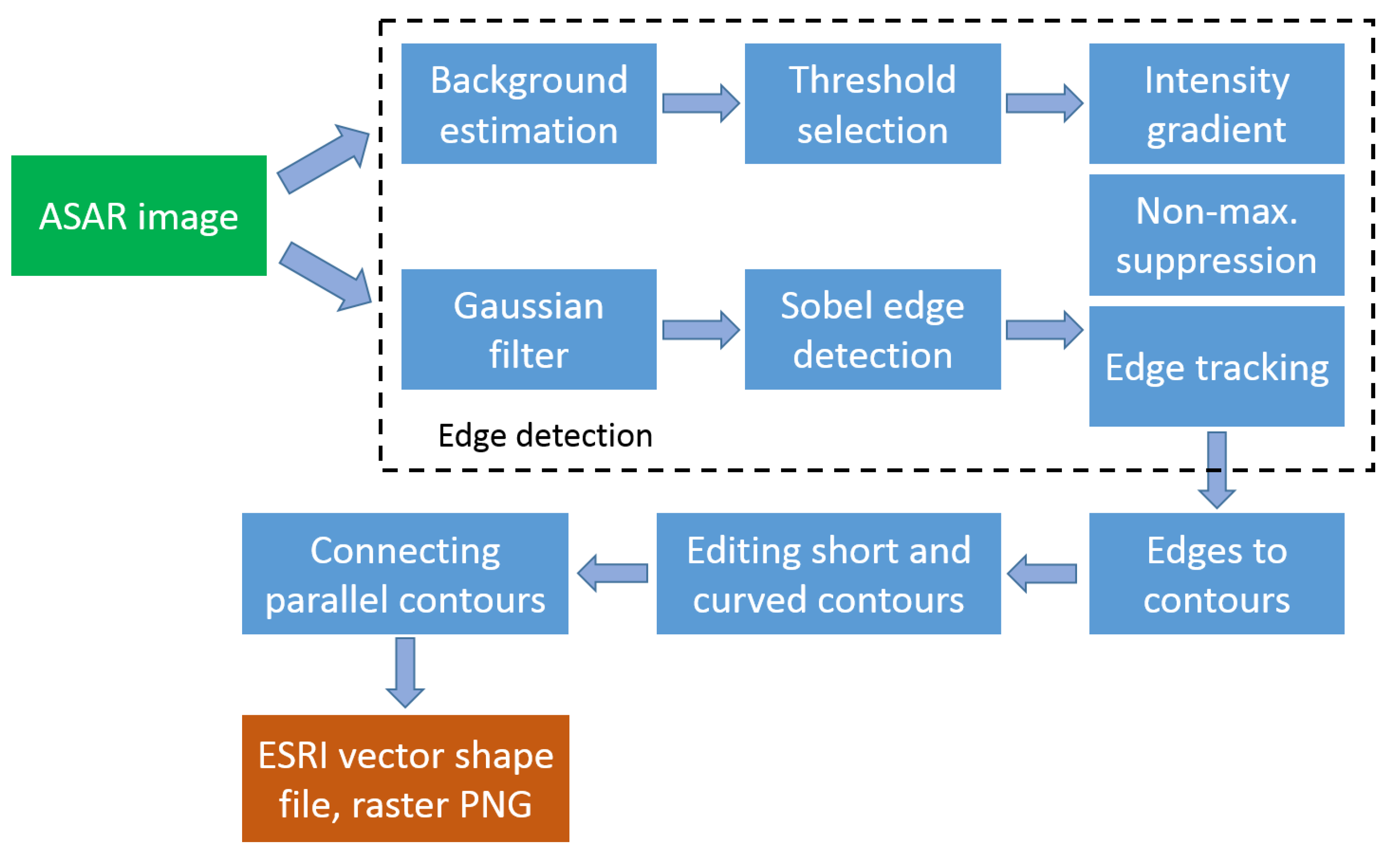
3.2.1. Implementing Canny Edge Detection

The Canny edge detection algorithm [15] consists of multiple stages: reducing noise using a Gaussian filter, then calculating the image gradient magnitude and direction. The edges are thinned by suppressing non-maximal gradients, then a final hysteresis stage retains weaker gradients only if they are connected to stronger gradient pixels along the edge.

This classic algorithm has been extended with additional stages for the IW edge analysis. At the first stage, the image background intensity level is estimated by applying a running window median filter of round shape and 60 pixels in diameter to the ASAR image, which is shown in Figure 5a. The filter outputs a smoothed image with removed ridge features and details, as illustrated in Figure 5b.

The smoothed image serves as the baseline for estimation of the image noise level and for the selection of the upper and lower thresholds of the Canny edge detection algorithm. The noise level is estimated by applying a multiplicative model where the noise level is proportional to the image intensity [21]. The multiplicative nature of noise in ASAR images is known as the speckle phenomenon, where the coherent combination of reflected signals with different phases and amplitudes produce random fluctuations [22]. The variance of the speckle noise ${\sigma }_{sp}^2$ in ASAR image is defined by the equivalent number of looks L and the average intensity I [23] as:

$${\sigma }_{sp}^2=I/L$$

(1)

It follows from (1) that the intensity of speckle noise increases with image intensity, so the threshold for Canny edge detection was selected accordingly to match these changes. The upper threshold T_U was calculated for every pixel location $\left(r,c\right)$ as:

$$T_U\left(r,c\right)=C_U·{\sigma }_{sp}\left(r,c\right)$$

(2)

where $C_U$ is a constant that defines the sensitivity of the edge detection algorithm and its false alarm rate. ${\sigma }_{sp}\left(r,c\right)$ is the variance of speckle noise at location $\left(r,c\right)$. A similar approach has been applied for the selection of the lower threshold T_L:

$$T_L\left(r,c\right)=C_L·{\sigma }_{sp}\left(r,c\right)$$

(3)

The $C_U$ and $C_L$ constants in (2) and (3) were selected by processing test ASAR images and visual assessment of detection results.

3.2.2. Algorithm Tuning

The algorithm for IW detection (Section 3.2.1) uses several parameters that affect its sensitivity and the false alarm rate. To achieve better performance and improve the accuracy of detection results, this algorithm has been additionally tuned using test ASAR images of IWs.

The test data we used were the scene in Figure 5a (Celtic Sea, 13 July 2011) chosen to have as many IWs as possible, and all scenes from 14 consecutive days during which no genuine IWs were observed visually (1–14 July 2009). Images of the original data superimposed with detected edges were manually inspected for errors, both false negative (where an IW-like edge was visible) and false positive (where no IW-like edge was visible, or it was not part of a wave train). Images were displayed at each stage of the algorithm, allowing us to see the effect of each stage. Before tuning, the default parameters were: lower Canny threshold $C_L=0.02$; upper Canny threshold $C_U=0.2$; smoothing sigma $\sigma =3$.

Based on previous experience of front detection, we tried upper Canny thresholds from 0.3 to 0.9 and a lower threshold of 0.1. The upper threshold of 0.5 detected some clear IW-like features not detected by higher thresholds, whereas 0.3 detected more IWs but significantly increased the number of false detections. We decided to err on the side of ensuring the detection of IWs with more false positives and filter out the false positives at a later stage of processing (Section 3.2.3). Further reducing the lower Canny threshold resulted in many more false positives with no apparent gain in IW detection. We did not try changing the smoothing sigma, as the chosen value was considered to be reasonable. Final parameters after tuning were: lower Canny threshold $C_L=0.1$; upper Canny threshold $C_U=0.3$; smoothing sigma $\sigma =3$. The resulting detected edges are shown in Figure 5c,d.

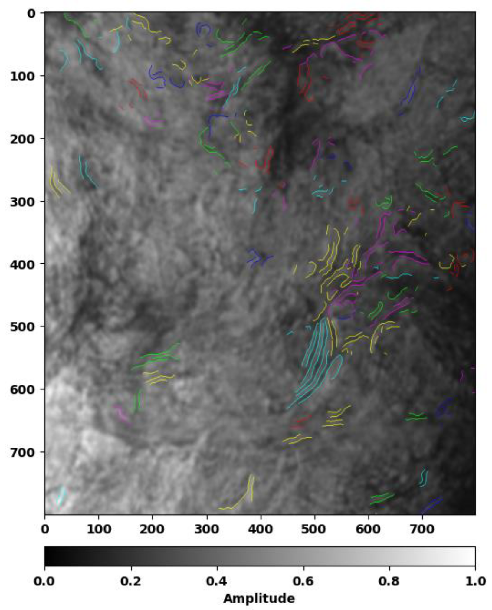
3.2.3. Filtering and Grouping of IWs

This proceeds in three distinct stages following Canny edge detection, as illustrated in Figure 6. The overarching idea behind this process is to join edges that we consider to belong to the same IW train and split edges at sharp discontinuities indicative either of a junction between two IWs or of a non-IW feature. Once this is done, we can select just the features most clearly belonging to IW trains.

In the first stage, Canny-detected edges are divided into clusters of connected line segments (Figure 5d), and clusters containing less than $N_{short}$ pixels are discarded. We have found that some scenes contain many very short, isolated fragments that can slow down processing considerably while contributing little or nothing to algorithm performance. The orientation of such fragments is difficult to determine, so they are often associated wrongly with other segments in the third stage below. Line segments are formed by ‘walking’ along edges, creating a break between segments if the line bends by ≥45° or we arrive at a previously encountered pixel. At triple points (junctions of three or more edges), the two most similarly oriented edges are considered part of the same segment unless they deviate by ≥45°. Each segment is then simplified by representing it as a number of straight facets, with each facet made as long as possible without deviating from the segment by more than 1 pixel. Facets within a segment are then combined into geometric elements (straight sections and circular arcs, depending on which best fits the segment data). Straight sections are drawn from end to end of the combined data, while arcs are drawn between the two ends and an intermediate vertex. If the angle between two adjacent elements is ≥45° the segment is split, and if an arc has a radius less than rmin, it is considered as a discontinuity and the segment is split before and after the arc. Results presented use parameter settings $N_{short}=5$ pixels and $r_{min}=5$ pixels (about 375 m).

In the second stage, segments that are longer than $N_{short}$ pixels and either within the same cluster or in a neighbouring cluster separated by less than $d_{max}$ pixels are considered for grouping, which takes place if the combination of two elements (one from each segment) into a single straight section or arc results in a better overall fit. Straight sections are drawn from either end of one element to either end of the other, while arcs use any three of the four ends. After connection, groups that are shorter than $N_{long}$ pixels are discarded. The algorithm uses parameter settings $d_{max}=20$ pixels and $N_{long}=25$ pixels.

In the third stage, parallel groups are connected. For each group A, all other groups B with facet vertices within $d_{seg}$ pixels of any part of group A are found using a KD-tree algorithm [24], then for each group B, the N pixels within $d_{seg}$ pixels of group A are considered. Their median distance $d_{med}$ and the number $N_{close}$ of distances within $x_{max}·d_{med}$ of $d_{med}$ are calculated. If $N_{close}$ is greater than $N_{min}$ and $N_{close}/N$ is greater than $p_{min}$, groups A and B are connected. The purpose of this is to find pairs of groups that have long sections separated by a consistent distance. The greater the separation of the groups, the more consistent their distance must be. Groups are only considered to be IWs if they are connected to at least one other group. Figure 7 shows the results of parallel groups identification. The following parameters were used: $d_{seg}=20$ pixels, $x_{max}=15$, $N_{min}=25$ and $p_{min}=0.5$.

3.3. Distribution of IWs

The factors that adversely affect the accuracy of IW contour maps such as Figure 7 are speckle noise in ASAR images, low contrast of IWs features and possibly false alarms at the output of the edge detection algorithm. To reduce these errors and improve the accuracy of IW mapping, we adopted a gridding approach based on combining the information in space and time. The satellite measurements were mapped into an evenly spaced grid of lower resolution and averaged over a time interval.

At the output of the detection algorithm, described in detail in Section 3.2, the contours of IWs were produced in vector format. To combine vector data spatially or in time, the contours were transformed into a raster format as follows. For each radar image, a raster image of exactly the same size was created filled with zero values, then IW contours (see Figure 7) were plotted on this image by using Bresenham’s line drawing algorithm, filling the grid with non-zero values in the locations where IWs were detected. These raster images were then composited in space and time to produce monthly, annual and seasonal composite maps of the distribution of IW occurrence. For this study, we adopted a spatial resolution of 10 × 10 arc minutes, or about 9 × 18 km at 60°N.

These maps show how frequently IWs were found in radar images. For each grid cell in the map, the frequency of IW occurrence was estimated as the ratio of detected IW pixels to the total number of radar image pixels. The frequency values were calculated for multiple radar images and then averaged in space and time as:

$$F_{i,j}=\left({\displaystyle \sum }_{k=1}^K{\displaystyle \sum }_{x\in X_i}{\displaystyle \sum }_{y\in Y_j}{w}_{x,y}\right)/\left(K·N\right),0\le i<I,0\le j<J$$

(4)

where k is the ASAR image index and K is the total number of composed images. i and j are row and column numbers of a grid element in the IW distribution map, and I,J are the total numbers of grid elements. (x,y) are the coordinates of a pixel in the ASAR image and X_i,Y_j is the subset of all ASAR pixels contained in grid element (i,j). The total number of pixels in the subset is denoted by N. The value of w_x,y is set to one if the IW was detected in the ASAR image pixel with coordinates (x,y), otherwise, it is set to zero.

The total number of ASAR images combined in Equation (4) is different for monthly, annual and seasonal IW distribution maps. For a one-month time interval, the average number of images is K ≈ 6 (Figure 2). The number of ASAR image pixels contained in each grid element of the IW distribution map depends on the map resolution and coordinates. With the 10 × 10 arc minute resolution adopted here, each grid cell covers around 250 × 130 ≈ 33,000 pixels. Hence, on average, ∼200,000 ASAR pixels can be composed to estimate the frequency parameter $F_{i,j}$ using Equation (4) for each grid element of a monthly IW distribution map. This makes the $F_{i,j}$ estimate more resistant to the false alarms generated by the IW detection technique, described in Section 3.2.

4. Results and Discussion

4.1. Distribution of IWs

The distribution of IWs in the UKCS was evaluated at different time scales and intervals. Monthly maps of IW occurrence were generated for each month in the years 2006–2012. The monthly maps provide the best time resolution, appropriate for observing ongoing changes in IW distribution. However, the number of sensor measurements averaged over one month is relatively small (see Section 2.2) and this affects the accuracy of the IW occurrence maps. Selected examples of monthly IW occurrence maps are shown in Figure 8. The frequency of IW in the maps is presented using a colour palette in the range from 0 (white) to 0.005 (dark red). Masked areas are shown in grey. As can be expected, a higher frequency of IW occurrence is observed along seabed topographic features, such as shelf breaks, ridges and troughs (see Figure 1). Figure 8a–d show proliferation of IWs observed at Dogger Bank in April 2007, the Wyville-Thomson Ridge in June 2008, at the edge of the continental shelf to the east of Rosemary Bank in January 2010 and in the Faroe-Shetland Channel in June 2011, respectively.

Figure 9 shows the IW occurrence map calculated using all data available over the period of ENVISAT ASAR observations from 2006 to 2012. The map indicates the importance of the Hatton-Rockall Basin and Wyville-Thomson Ridge in the generation of IWs. The comparison of annual maps with monthly data (Figure 8) also shows high interannual and seasonal variability of IWs in the UKCS.

Annual composite maps of IW occurrence are presented in Figure 10 for the years 2006–2012. It is seen from these maps that over the whole year, IWs are mostly present in the Hatton-Rockall Basin and Hatton Bank. The most significant years in terms of IW activity were 2006, 2010 and 2011.

Monthly climatology maps of IW occurrence are presented in Figure 11. The maps were generated by combining the same month over the years 2006 to 2012. These show that a higher intensity of IWs is observed in the spring and summer periods. These observations agree with the seasons when the UKCS waters are more stratified [25].

IWs can travel hundreds of km from their source, so IW occurrence is not expected to be directly related to bathymetry, but it is of interest to see whether IWs are detected more often at certain depths. Figure 12 shows a bar chart of the mean IW occurrence as a function of bottom depth, binned at 20 m intervals. This indicates that IW occurrence shows no depth trend between about 900 m and 2500 m, increasing markedly from 900 m to shore and from 2750 m to the deepest waters in the UKCS at 3160 m.

4.2. Evaluation Results

We visually inspected all monthly IW occurrence maps to identify patterns of IW occurrence (see Supplementary Material to access the maps). IW-like features are detected consistently throughout the year very close to the coast, though many of these near-coast detections are likely to be false positives due to the interaction of surface waves with the coastal bathymetry. Further from the coast, we can be more confident in our results. There follows a list of the most prominent non-coastal IW detection features seen in Figure 9, Figure 10 and Figure 11 in the UKCS, from west to east. The features are denoted with letters and their locations are shown in red in Figure 9. Selected features are shown in closeup in Figure 13.

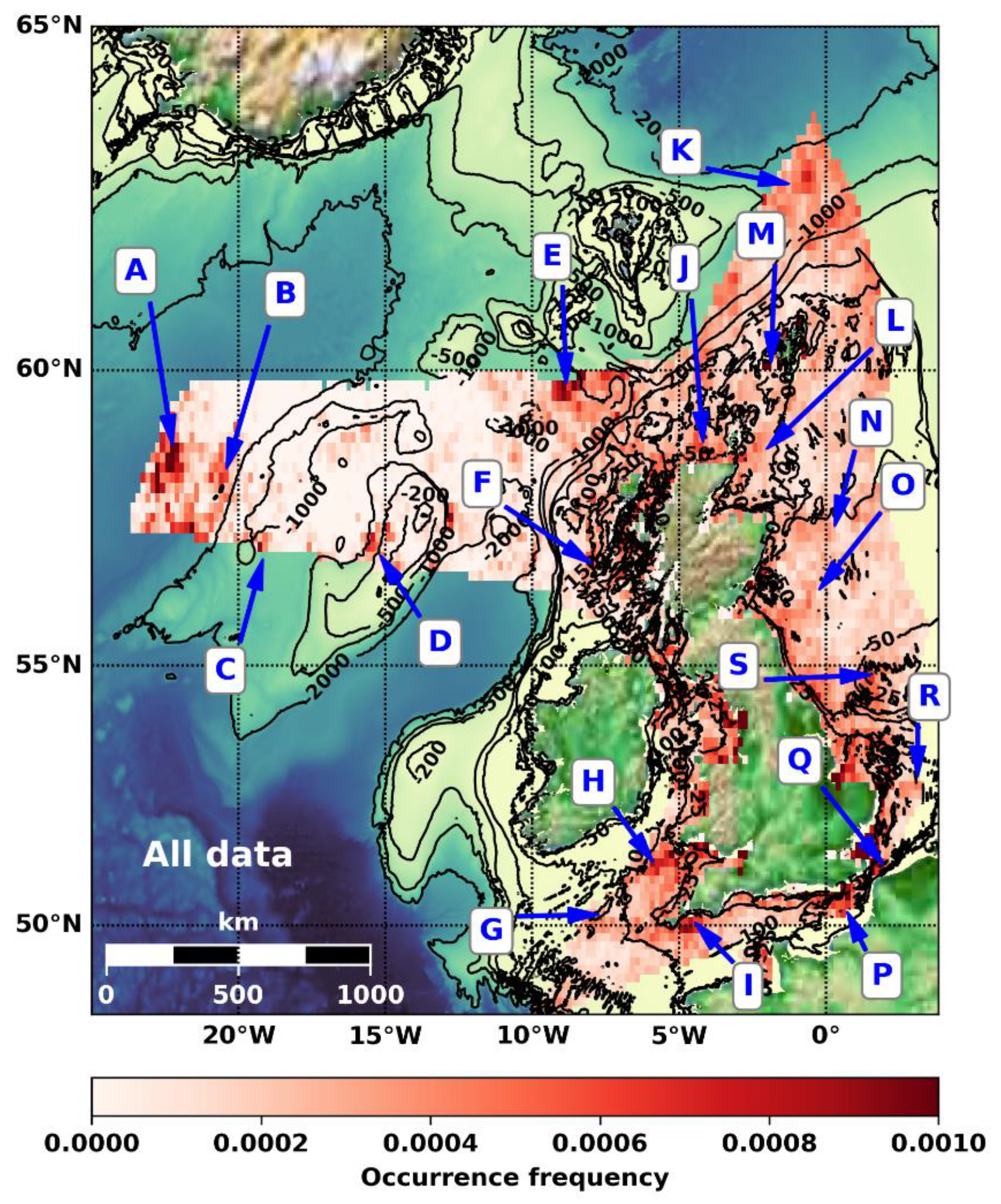
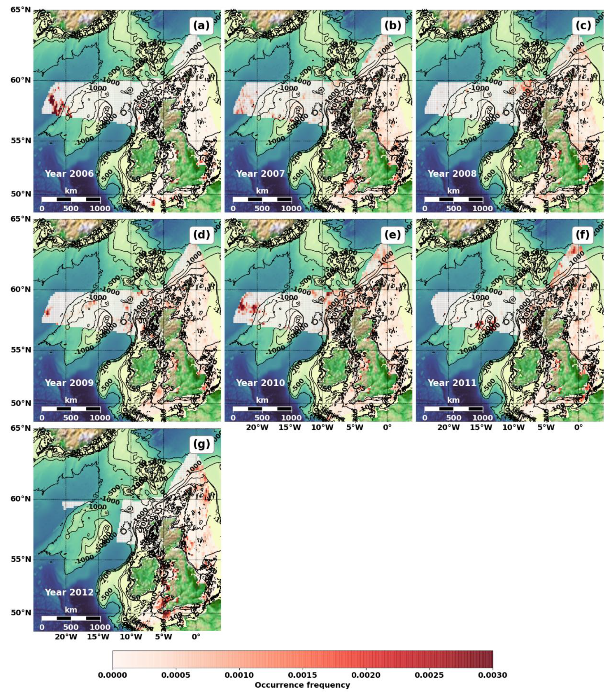
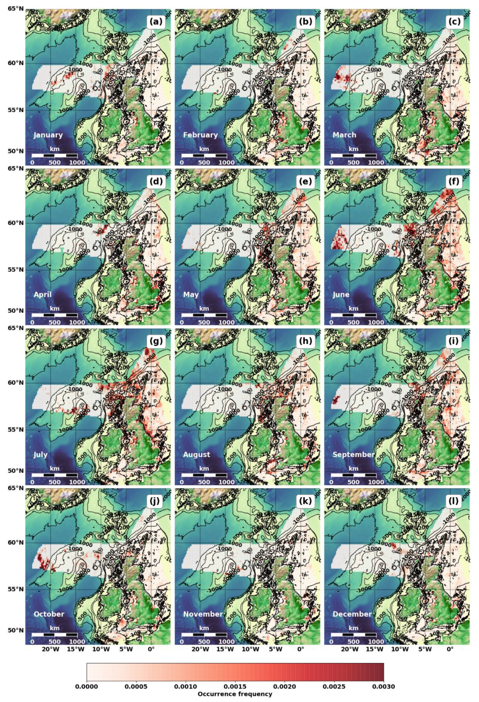
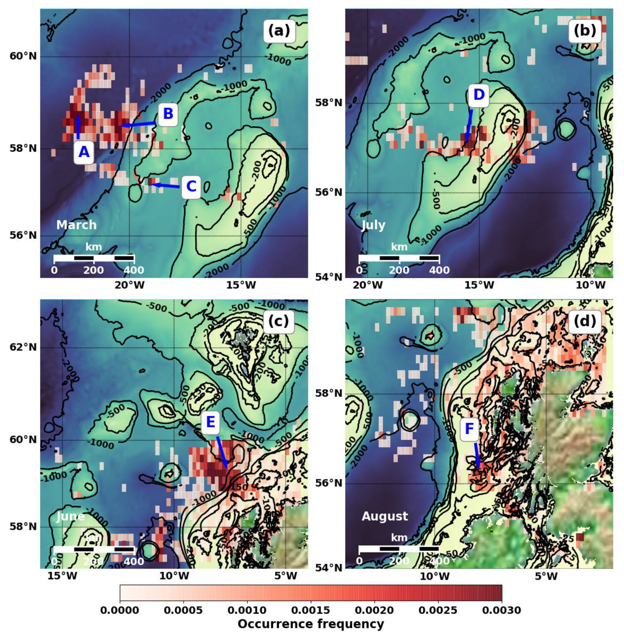
• A (see Figure 13a): A very strong, localised feature is visible close to the westernmost extremity of the UKCS in the Iceland Basin, centred on about 58° 30′N, 22° 30′W in waters around 3000 m deep, around 150 km from the nearest bathymetric feature, Hatton Bank, which at its shallowest is around 500 m deep. This feature appears mainly in 2006, 2010 and weakly in 2009, most strongly in March and October, slightly further south in September and in a more dispersed form in June.
• B (see Figure 13a): Separated from feature A to the east is a generally more dispersed feature that runs along the western edge of Hatton Bank between the southern edge of the UKCS at about 57°N, 22°W and about 59°N, 20°W, appearing in 2006 and 2010 and in the same months except in September. This suggests that the features are related, e.g., non-horizontally-propagating IWs may be generated at the edge of Hatton Bank and propagate down to the seafloor and back up to the Icelandic Basin.
• C (see Figure 13a): A small, distinct feature is visible on the southern edge of Hatton Bank at the edge of the UKCS at about 57°N, 19°W, appearing strongly in October 2006, with weaker features dispersed northwards from this feature along the southern edge of Hatton Bank to about 59°N, 15°W, appearing strongly in January 2009.
• D (see Figure 13b): A weak, dispersed feature is visible at the western edge of the Rockall Bank at about 57°N, 15° 30′W, appearing strongly in July 2011.
• E (see Figure 13c): A strong, localised feature is visible at the southern edge of the Faroe Bank at the edge of the UKCS at about 60°N, 9°W, appearing mostly in 2009–2010 from April–August.
• F (see Figure 13d): A weak linear feature runs N-S on the Hebridean Shelf west of the Outer Hebrides from 56 to 58°N, 8°W, at about 100 m depth, appearing mostly in 2009 and 2011, most strongly in May and July, also in August–September.
• G: A weak linear feature runs E-W on the Celtic Shelf at 50°N from Jones Bank at the edge of the UKCS at about 8°W to Land’s End at 6°W, at about 100 m depth, appearing in 2007, 2009 and 2011 in March–April and July–September.
• H: A stronger linear feature runs north of the Bristol Channel from about 51°N, 7°W to the southwestern tip of Wales at 51°30′N, 6°W, at 50 to 120 m depth, appearing strongly with distinct linearity in August 2007.
• I: A small, distinct feature is visible off the Lizard peninsula in Cornwall at 50°N, 5°W, at 80 to 90 m depth, appearing strongly in March 2012.
• J: A small feature is visible off the north coast of Scotland at about 58°N, 4°W, at 60 to 90 m depth, appearing in 2009–2011, most strongly in July and December.
• K: A broad region of indistinct features is visible in and on the southeast edge of the Faroe-Shetland Channel, northwest of a line between 59°N, 5°W and the edge of the UKCS at 62°N, 2°E, appearing in variable locations in 2007–2012, mostly in May–July and strong features in the middle of the Channel in February 2007 and in the north in June–July 2011.
• L: Another broad feature extends from the northeast tip of Scotland at 58°30′N, 3°W to the northeast, passing southeast of Shetland and across Viking Bank to the edge of the UKCS at 61°30′N, 2°E, close to the Norwegian Trough, at 50 to 180 m depth, appearing mainly in 2011–12 but also in 2008–2010, very distinctly in September, less so in May-August and faintly through most of the year.
• M: A strong, highly distinct feature visible in a fixed location west of Shetland at 60°N, 2°W, appearing equally in all years and months and probably an artefact relating to the island of Foula.
• N: A broad, weak feature is visible east of Scotland centered on 57°30′N, 1°W, at 60 to 120 m depth, appearing in 2007–2009 and 2011, most strongly in September but also from May–August.
• O: A broad feature is visible extending from the Northumberland coast at 55°30′N, 1°30′W to 56°N, 30′W at 50 to 90 m depth, appearing from 2007–2012 in March, May–July and September–October.
• P: A small but strong feature is visible off the south Kent coast at 50°30′N, 1°E at about 30 m depth, appearing in 2010–2011 in March, July–August and October.
• Q: A very strong feature, visible in a fixed location in the Thames estuary centered on 51°30′N, 2°E at 10 to 20 m depth and appearing throughout the year is probably an artefact due to artificial structures.
• R: A broad, weak feature is visible east of the Humber centred on 53°30′N, 2°E at 15 to 30 m depth, appearing in most years and months but most strongly in 2006 and 2010–2011 and in April. At this depth, and with this consistency of appearance, it is possible that the feature is due to seabed effects on surface waves.
• S: A broad feature is visible over Dogger Bank at 54°30′N, 2°E at 15 to 25 m depth, appearing in all years and most months, most strongly from March to July. At this depth, and with this consistency of appearance, it is possible that the feature is due to seabed effects on surface waves.

The features identified at the UK continental shelf using IW occurrence maps were compared to observations presented in other studies. The Atlas of Internal Solitary-like Waves [26] indicates IW activity in the Faroe-Shetland Channel and at Rockall Bank and the north and west coasts of Scotland. These locations are in good agreement with features K, D and J, respectively in Figure 9. The spatial resolution of IW occurrence maps in the atlas is at least 10 times lower than the resolution of the maps generated in this study and many features observed here were missing in the atlas. More detailed information was provided through in situ measurements and modelling experiments carried out in [27,28,29,30,31]. Three main areas were identified in the literature as IW hotspots: the Malin Shelf, the Wyville-Thomson Ridge and Jones Bank in the Celtic Shelf.

Detailed studies of IWs at the Malin Shelf were carried out by Small et al. in [27] using acoustic measurements and SAR data. It was shown that in summer IWs are a common feature in this region. These observations also match with the IW hotspot F in this region in Figure 13d. This feature can also be clearly seen in the climatology maps in July and August (Figure 11g,h). Vlasenko et al. [28] carried out numerical modelling of IW at the Malin Shelf and provided further insight into the behaviour of IWs in this region. This study describes two wave processes developing in this area: a tidal beam generated at the shelf break and the bottom trapped internal waves generated by the tidal flow over local seabed features.

Another IW hotspot studied in the literature is the Wyville-Thomson Ridge. The numerical simulation results performed by Hall et al. [29] indicated the presence of internal tides in this region. Vlasenko et al. [30] carried out a detailed analysis of water circulation at the ridge that demonstrated favourable conditions for IWs.

Internal waves in the Celtic Sea have been studied in situ and with numerical modelling. Vlasenko et al. [31] carried out numerical modelling of the interaction of stratified tidal flows with the seabed at Jones Bank and found that tidal currents can generate two types of IWs. Palmer et al. [32] carried out in situ observations at Jones Bank and revealed IWs of up to 40 metres in amplitude occurring during spring periods. Feature G in Figure 9 shows a high occurrence of IWs around Jones Bank.

5. Conclusions

In this work, a methodology has been developed for processing satellite SAR sensor data to map internal waves in the UK Continental Shelf. We have made significant advances on previous approaches by implementing automated detection of the IW features. This has the advantage of speeding up the analysis, enabling thousands of SAR images to be processed rather than tens. It also avoids the tedious and subjective manual/visual detection of IW packets, a critical factor in the generation of an accurate and comprehensive distribution map.

We provide the first detailed and systematic distribution maps of IW occurrence across the UKCS by processing a 7-year time series of ENVISAT ASAR sensor data, acquired by the European Space Agency. Overall, the IW occurrence maps demonstrate good agreement with previous findings and with prominent non-coastal seabed topographic features. The comparison of annual and monthly IW maps reveals high interannual and seasonal variability of IWs in the UKCS.

Features revealed by this work could be investigated further by construction of time series of IW occurrence in a region of interest, followed by manual examination of the scenes contributing to each feature to check for artefacts due to meteorological events (e.g., convective storms or atmospheric gravity waves), or consistent features indicative of a permanent structure in the water. As structures such as wind farms or oil platforms are placed in or removed from UKCS waters, time series analysis may also reveal the effect of these structures on IW occurrence.

Future work will address adapting the methodology to exploit SAR datasets produced by other sensors. For example, ESA’s Sentinel-1A and 1B paired sensors would offer an improvement in revisit time, spatial resolution and continuity of IW observations. The advance we have demonstrated in this automated and robust algorithm should be widely applicable to studies of the distribution and impact of internal waves in other regions around the world.

References

1. Rodenas, J.A.; Garello, R. Wavelet analysis in SAR ocean image profiles for internal wave detection and wavelength estimation. IEEE Trans. Geosci. Remote Sens. 1997, 35, 933–945. [Google Scholar] [CrossRef]
2. Changbao, Z.; Jingsong, Y.; Weigen, H.; Bin, F.; Aigin, S.; Donglin, L. Satellite SAR Remote Sensing of Ocean Internal Waves. In Proceedings of the 20th Asian Conference on Remote Sensing (ACRS), Hong Kong Convention and Exhibition Centre, Hong Kong, China, 22–25 November 1999; p. 5. [Google Scholar]
3. Rodenas, J.; Garello, R. Internal wave detection and location in SAR images using wavelet transform. IEEE Trans. Geosci. Remote Sens. 1998, 36, 1494–1507. [Google Scholar] [CrossRef]
4. Simonin, D.; Tatnall, A.R.; Robinson, I.S. The automated detection and recognition of internal waves. Int. J. Remote Sens. 2009, 30, 4581–4598. [Google Scholar] [CrossRef]
5. Bao, S.; Meng, J.; Sun, L.; Liu, Y. Detection of ocean internal waves based on Faster R-{CNN} in SAR images. J. Oceanol. Limnol. 2020, 38, 55–63. [Google Scholar] [CrossRef]
6. Dokken, S.T.; Olsen, R.; Wahl, T.; Tantillo, M.V. Identification and characterization of internal waves in SAR images along the coast of Norway. Geophys. Res. Lett. 2001, 28, 2803–2806. [Google Scholar] [CrossRef]
7. Zhao, Z.; Klemas, V.; Zheng, Q.; Yan, X.H. Remote sensing evidence for baroclinic tide origin of internal solitary waves in the northeastern South China Sea. Geophys. Res. Lett. 2004, 31. [Google Scholar] [CrossRef] [Green Version]
8. Lorenzzetti, J.A.; Dias, F.G. Internal Solitary Waves in the Brazilian SE Continental Shelf: Observations by Synthetic Aperture Radar. Int. J. Oceanogr. 2013, 2013, 403259. [Google Scholar] [CrossRef] [Green Version]
9. Kozlov, I.E.; Kudryavtsev, V.N.; Zubkova, E.V.; Zimin, A.V.; Chapron, B. Characteristics of short-period internal waves in the Kara Sea inferred from satellite SAR data. Izv. Atmos. Ocean. Phys. 2015, 51, 1073–1087. [Google Scholar] [CrossRef]
10. Lavrova, O.; Kostianoy, A. Spatio-temporal variability of internal waves in the Caspian Sea, European Geosciences Union EGU 2020. Available online: https://meetingorganizer.copernicus.org/EGU2020/EGU2020-10011.html (accessed on 8 June 2020).
11. Zhou, L.; Yang, J.; Wang, J.; He, S.; He, Z.; Liu, A.K.; Hsu, M.-K. Spatio-temporal distribution of internal waves in the Andaman Sea based on satellite remote sensing. In Proceedings of the 2016 9th International Congress on Image and Signal Processing, BioMedical Engineering and Informatics (CISP-BMEI), Datong, China, 15–17 October 2016; IEEE: Piscataway, NJ, USA, 2016. [Google Scholar] [CrossRef]
12. Ning, J.; Sun, L.; Cui, H.; Lu, K.; Wang, J. Study on characteristics of internal solitary waves in the Malacca Strait based on Sentinel-1 and GF-3 satellite SAR data. Acta Oceanol. Sin. 2020, 39, 15–156. [Google Scholar] [CrossRef]
13. Mitnik, L.M.; Khazanova, E.S.; Dubina, V.A. Mesoscale and synoptic scale dynamic phenomena in the Oyashio current region observed in SAR imagery. Int. J. Remote Sens. 2019, 41, 5861–5883. [Google Scholar] [CrossRef]
14. Gede, I.G.; Chonnaniyah, K.A.; Osawa, T. Internal solitary wave observations in the Flores Sea using the Himawari-8 geostationary satellite. Int. J. Remote Sens. 2019, 41, 5726–5742. [Google Scholar] [CrossRef]
15. Canny, J. A computational approach to edge detection. IEEE Trans. Pattern Anal. Mach. Intell. 1986, 8, 679–698. [Google Scholar] [CrossRef] [PubMed]
16. Narayanaswamy, B.E.; Bett, B.J.; Hughes, D.J. Deep-water macrofaunal diversity in the Faroe-Shetland region (NE Atlantic): A margin subject to an unusual thermal regime. Mar. Ecol. 2010, 31, 237–246. [Google Scholar] [CrossRef]
17. Watson, R.; Albon, S.; Aspinall, R.; Austen, M.; Bardgett, B.; Bateman, I.; Berry, P.; Bird, W.; Bradbury, R.; Brown, C. UK National Ecosystem Assessment: Technical Report; United Nations Environment Programme World Conservation Monitoring Centre: Cambridge, UK, 2011. [Google Scholar]
18. GEBCO Bathymetric Compilation Group. The GEBCO_2020 Grid—A Continuous Terrain Model of the Global Oceans and Land; British Oceanographic Data Centre; National Oceanography Centre; NERC: Liverpool, UK, 2020. [Google Scholar] [CrossRef]
19. Ward, K.D.; Tough, R.J.A.; Watts, S. Sea clutter: Scattering, the K distribution and radar performance. Waves Random Complex Media 2007, 17, 233–234. [Google Scholar] [CrossRef]
20. European Space Agency. ASAR Product Handbook, ESA 2007, Issue 2.2. Available online: http://envisat.esa.int/handbooks/asar/CNTR.html (accessed on 8 June 2020).
21. Ulaby, F.T.; Moore, R.K.; Fung, A.K. Microwave Remote Sensing Active and Passive-Volume II: Radar Remote Sensing and Surface Scattering and Emission Theory; Addison-Wesley: Boston, MA, USA, 1982; 628p, ISBN-13: 978-0890061916. [Google Scholar]
22. Kulemin, G.P. Millimeter-Wave Radar Targets and Clutter; Artech House: Boston, MA, USA, 2003; 344p, ISBN-13: 978-1580535403. [Google Scholar]
23. Oliver, C.; Quegan, S. Understanding Synthetic Aperture Radar Images; SciTech Publishing: Raleigh, NC, USA, 2004; 510p, ISBN-13: 978-1891121319. [Google Scholar]
24. Goodman, J.E.; O’Rourke, J. Chapter 43: Nearest neighbours in high-dimensional spaces. In Handbook of Discrete and Computational Geometry, 3rd ed.; Goodman, J.E., O’Rourke, J., Csaba, D.T., Eds.; CRC Press LLC: Boca Raton, FL, USA, 2017; pp. 1135–1155, ISBN-13: 978-1584883012. [Google Scholar]
25. Elliott, A.J.; Clarke, T. Seasonal stratification in the northwest European shelf seas. Cont. Shelf Res. 1991, 11, 467–492. [Google Scholar] [CrossRef]
26. Jackson, C.R. Northeast Atlantic. In An Atlas of Internal Solitary-like Waves and Their Properties, 2nd ed.; Global Ocean Associates: Alexandria, VA, USA, 2004; pp. 121–150. Available online: http://www.internalwaveatlas.com/Atlas2_index.html (accessed on 23 July 2020).
27. Small, J.; Hallock, Z.; Pavey, G.; Scott, J. Observations of large amplitude internal waves at the Malin Shelf edge during SESAME 1995. Cont. Shelf Res. 1999, 19, 1389–1436. [Google Scholar] [CrossRef]
28. Stashchuk, N.; Vlasenko, V. Bottom trapped internal waves over the Malin Sea continental slope. Deep Sea Res. Part I Oceanogr. Res. Pap. 2017, 119, 68–80. [Google Scholar] [CrossRef] [Green Version]
29. Hall, R.A.; Huthnance, J.M.; Williams, R.G. Internal tides, nonlinear internal wave trains, and mixing in the Faroe-Shetland Channel. J. Geophys. Res. 2011, 116, 1–15. [Google Scholar] [CrossRef]
30. Vlasenko, V.; Stashchuk, N. Tidally Induced Overflow of the Faroese Channels Bottom Water Over the Wyville Thomson Ridge. J. Geophys. Res. Oceans 2018, 123, 6753–6765. [Google Scholar] [CrossRef]
31. Vlasenko, V.; Stashchuk, N.; Palmer, M.R.; Inall, M.R. Generation of baroclinic tides over an isolated underwater bank. J. Geophys. Res. Oceans 2013, 118, 4395–4408. [Google Scholar] [CrossRef] [Green Version]
32. Palmer, M.R.; Inall, M.E.; Sharples, J. The physical oceanography of Jones Bank: A mixing hotspot in the Celtic Sea. Prog. Oceanogr. 2013, 117, 9–24. [Google Scholar] [CrossRef]
Figure 1. Map of the study region. The borders of the UK continental shelf (UKCS) are shown in red solid lines. The bathymetry is taken from the General Bathymetric Chart of the Oceans (GEBCO) dataset [18]. The sea depth is displayed in a dark-blue and yellow palette and with black contour lines at intervals 25, 50, 100, 150, 200, 500, 1000, 2000 m. The seabed topographical features are shown in blue text.
Remotesensing 12 02476 g001
Figure 2. The average revisit time in days for the ENVISAT ASAR sensor within the UK continental shelf as a function of a month. The estimate is based on ENVISAT scenes acquired in 2006–2012.
Remotesensing 12 02476 g002
Figure 3. The average time in days between satellite observations in the UKCS.
Remotesensing 12 02476 g003
Figure 4. ENVISAT ASAR data processing chain. The original ASAR images are initially split into tiles of smaller size to improve performance. The algorithm for IW detection is applied before image mapping to geographical coordinates.
Remotesensing 12 02476 g004
Figure 5. (a) ENVISAT ASAR image of the Celtic Sea on 13 July 2011 at 22:18; (b) background image after median filtering; (c) after Gaussian filtering with a filter standard deviation of 3; (d) detected edges, with connected clusters of edges shown in different colours.
Remotesensing 12 02476 g005
Figure 6. Block diagram of ASAR satellite image processing and internal wave detection technique. The processing chain is split into two parallel branches in which threshold selection and Sobel edge detection are applied.
Remotesensing 12 02476 g006
Figure 7. Parallel groups of internal wave features. Each set of parallel groups has its own colour. The total number of candidates for IW contours has reduced significantly after filtering and grouping stages.
Remotesensing 12 02476 g007
Figure 8. Selected monthly maps of internal wave occurrence. The frequency of internal wave occurrence is shown with a white and red palette and ranges from 0 to 0.005. The maps demonstrate high seasonal variability of IWs: (a) IWs at Dogger Bank and Faroe-Shetland Channel in April 2007; (b) IWs at Wyville-Thompson Ridge in June 2008; (c) IWs at Wyville-Thompson Ridge and Celtic Shelf in January 2010; (d) IWs at Faroe-Shetland Channel in June 2006.
Remotesensing 12 02476 g008
Figure 9. Internal wave occurrence map of the UK continental shelf for the years 2006–2012, derived automatically from SAR data. The blue labels show regions with high occurrence if IW, identified by visual inspection of occurrence maps (see Section 4.2 for details). The occurrence frequency is shown using gradations of white and red.
Remotesensing 12 02476 g009
Figure 10. Annual maps of internal wave occurrence: (ag) in years 2006–2012.
Remotesensing 12 02476 g010
Figure 11. Monthly climatology maps of internal wave occurrence: (al) from January to December.
Remotesensing 12 02476 g011
Figure 12. Bar chart of mean internal wave occurrence against water depth. Each bar shows the mean occurrence in a 20 m depth interval.
Remotesensing 12 02476 g012
Figure 13. Closeup maps of monthly climatological internal waves occurrence from Figure 11. Blue labels show locations of: (a) A, B and C features in the Iceland Basin and Hatton-Rockall Basin; (b) D feature in Hatton-Rockall Basin; (c) E feature at Wyville-Thompson Ridge; (d) F feature west of the Outer Hebrides. Occurrence frequency values < 0.0001 have been omitted from the map for clarity.
Remotesensing 12 02476 g013