Article

A New Approach for Understanding Urban Microclimate by Integrating Complementary Predictors at Different Scales in Regression and Machine Learning Models

UMR CNRS 5600 Environment, City and Society, Department of Geography and Spatial Planning, University Jean Moulin Lyon 3, 69007 Lyon, France
*
Author to whom correspondence should be addressed.
Remote Sens. 2020, 12(15), 2434; https://doi.org/10.3390/rs12152434
Submission received: 1 June 2020 / Revised: 10 July 2020 / Accepted: 13 July 2020 / Published: 29 July 2020
(This article belongs to the Special Issue Remote Sensing in Applications of Geoinformation)

Abstract

:
Climate change is a major contemporary phenomenon with multiple consequences. In urban areas, it exacerbates the urban heat island phenomenon. It impacts the health of the inhabitants and the sensation of thermal discomfort felt in urban areas. Thus, it is necessary to estimate as well as possible the air temperature at any point of a territory, in particular in view of the ongoing rationalization of the network of fixed meteorological stations of Météo-France. Understanding the air temperature is increasingly in demand to input quantitative models related to a wide range of fields, such as hydrology, ecology, or climate change studies. This study thus proposes to model air temperature, measured during four mobile campaigns carried out during the summer months, between 2016 and 2019, in Lyon (France), in clear sky weather, using regression models based on 33 explanatory variables from traditionally used data, data from remote sensing by LiDAR (Light Detection and Ranging), or Landsat 8 satellite acquisition. Three types of statistical regression were experimented: partial least square regression, multiple linear regression, and a machine learning method, the random forest regression. For example, for the day of 30 August 2016, multiple linear regression explained 89% of the variance for the study days, with a root mean square error (RMSE) of only 0.23 °C. Variables such as surface temperature, Normalized Difference Vegetation Index (NDVI), and Modified Normalized Difference Water Index (MNDWI) have a strong impact on the estimation model. This study contributes to the emergence of urban cooling systems. The solutions available vary. For example, they may include increasing the proportion of vegetation on the ground, facades, or roofs, increasing the number of basins and water bodies to promote urban cooling, choosing water-retaining materials, humidifying the pavement, increasing the number of public fountains and foggers, or creating shade with stretched canvas.

1. Introduction

Climate change is a major current phenomenon with multiple environmental, social and economic consequences [1]. In urban areas, it exacerbates the urban heat island (UHI) phenomenon [2,3] which is characterized by a difference in temperature between an urban area and the surrounding rural areas. In this case, the temperature in urban areas is higher than in rural areas, particularly at night [4,5]. The factors that contribute to heat intensification and UHI can be explicated mainly by the surface factors linked to the substitution of water surfaces, vegetation cover, and wetlands by artificial areas, causing low evaporation and evapotranspiration [6,7,8,9,10,11,12]. Buildings made of low-albedo materials with high thermal inertia capture, stock, and discharge the heat trapped with a thermal lag of several hours depending on the size and type of buildings and the climate [13]. This result is combined with the effect caused by structures made of low albedo supplies with high thermal inertia, which absorb and accumulate heat. The intensification of heat can also be caused by morphological parameters related to urban roughness and the sky-view factor (SVF) [14,15,16]. Indeed, the roughness can cause a diminution of the wind speed and the SVF can reduce the release of heat during the night [2]. Finally, anthropogenic parameters such as industrial heat emissions, heating, transport, or air conditioning can contribute as well to heat intensification [17,18,19,20], the “cities consume 78 percent of the world’s energy and produce more than 60 percent of greenhouse gas emissions. However, they account for less than 2 percent of the Earth’s surface” [21].
These two climatic manifestations have consequences on the health of the inhabitants [22] and on the sensation of thermal discomfort felt in urban areas [23,24]. Moreover, the increase in heat waves is clearly demonstrated, whether we look at the duration, intensity, or frequency [25]. The effects of heat waves are overlaid on the microclimatic characteristics of urban environments [26,27], as well as on the increasing urbanization process of the population. This increasing urbanization has a significant impact on urban microclimates and leads to warmer temperatures in cities [28,29,30,31]. One of the effects of the combination of these events is an increase in the premature number of heat stress related deaths [32]. In this context, local public actors are trying to prevent and reduce the human risks potentially generated by an increase in heat waves. Knowing and understanding the effect of the urban heat island is a key requirement for smart and sustainable city design [33]. According to the US Department of Energy, the United States spends $10 billion annually on energy to reduce the urban heat island effect [34]. In addition, mitigating urban overheating is an important financial issue since every 1 °C increase in temperature leads to a 2% to 4% increase in electricity demand [35]. In some regions, this increase would even vary between 0.45% and 4.6%, which would correspond to an additional electrical penalty of about 21W per degree of temperature increase per person [36]. This difference in energy consumption between urban and rural areas is mainly due to the fact that the cooling load of urban buildings is 13% higher than that of similar buildings in rural areas [37]. Thus, this relationship between electricity consumption and temperature has been clearly established [38]. In addition, a study in Chicago showed that adding 10% ground cover, or planting about three trees per plot of land, reduces energy costs by about $50–$90 (about 45–80 euros) per year per home [39].
In addition, air temperature is a main variable in explaining environmental conditions, especially urban conditions. It is also involved in many important ecological processes such as actual and potential evapotranspiration, net radiation, or the distribution of species [40]. Thus, knowledge of air temperature at any point in the territory is increasingly in demand to feed quantitative models related to a wide range of fields, such as hydrology, ecology [41], or climatology [42,43,44].
Consequently, the comprehension of air temperature models is essential for multiple applications in hydrology, land-use planning, or public health. Accurate knowledge of temperatures is a necessity both for the environment and for health policies, particularly in urban areas, which can contribute to improved urban planning in the context of UHI mitigation, and the creation of urban cooling islands (UCIs).
Thus, it is necessary to estimate the air temperature at any point in a territory as well as possible. This knowledge is directly dependent on the density of the measurement network, especially in view of the current rationalisation of the network of fixed meteorological stations of Météo-France [45]. In France, there are only a few agglomerations with their own network of fixed meteorological stations, such as Rennes and Dijon [46,47]. The air temperature evolving on a metric scale, at less than 100 meters [48,49], a very dense measurements network is needed. However, this is not the case in Lyon, which is the study area. Consequently, this study proposes to model air temperature using traditionally used data, data from remote sensing by LiDAR (Light Detection and Ranging), or Landsat 8 satellite acquisition and data produced by mobile measurement. These mobile measurements are very useful, as there is not yet a network of fixed weather stations sufficiently developed in Lyon, as in most large conurbations. In addition, the use of information obtained from airborne sensors or satellites to observe the earth’s surface from the sky or from space is a methodology that effectively evaluates the spatial distribution of land surface variables at the local and regional scales [50] and can be used for temperature modelling.
Urban air temperature can be estimated using different interpolation techniques such as spline [51,52] and interpolation kriging. More recently, modelling by regression [51] or by neural networks and other machine learning techniques has emerged [53]. Multiple studies have addressed this issue, either by using classical spatial interpolations (deterministic [54] or stochastic [55]) or by multiple regressions [42,50,56,57,58,59]. Previous air temperature modelling studies in urban areas are mostly based on measurements from fixed stations [42,47,52,60,61,62]. Studies involving modelling based on mobile measurements are less common [49,63]. Moreover, there have been none in the study area, whether they involve modelling from fixed stations or mobile measurements. Thus, this study has a double focus: to provide a first modelling of the air temperature of the territory using mobile measurements.
Most of the studies based on mobile measurements have been carried out using automobiles, for example in Portland (USA) [63], in Nancy (France) [44,64], in Los Angeles (USA) [65], in Hong-Kong [66], in Brno (Czech Republic) [67], or in Sfax (Tunisia) [68,69,70]. However, there are many inherent limitations of motorized transport. An increase in temperature may be observed when the car stops or slows down due to red lights or traffic jams. The proximity of other cars combined with the immobility of the vehicle may explain this. On the contrary, when the speed of the car increases, cooler temperatures may be observed due to the cooling of the speed of travel. Thus, this measurement method limits the route to be monitored because of the many one-way streets or pedestrian areas. Consequently, in this study, the choice to do bicycle measurements was made. These bicycle measurements already exist but are not so frequent. For example, they have been used in some areas such as in Rotterdam (Netherlands) [71], in Shenzhen (China) [72], in Ohio [73], in Utrecht (Netherlands) [74], and on foot in Vancouver (Canada) [49].
Moreover, the explanatory variables used for modelling air temperature are, in many cases, those commonly used such as latitude, longitude, altitude, and slope [60,75,76], or even the land use land cover [77]. Only some studies integrate some remote sensing data such as Difference Vegetation Index (NDVI) or Normalized Difference Moisture Index (NDMI) [49,63,78]. This study therefore proposes to reproduce, as well as possible, the conditions encountered in the field as a function of the morphological diversity very present in the urban environment using the largest possible sample of explanatory variables.
To summarize, the implications of this new approach for the understanding of urban micro-climates are fourfold. Firstly, mobile measurements to acquire air temperature are used on the second French conurbation, which has never been thermally modelled, despite marked thermal discomfort. Then, this air temperature will be modelled with a very large sample of explanatory variables, including classic topo climatic variables (altitude, longitude, latitude, slope, exposure, and so on), variables derived from the characteristics of the urban morphology (sky view factor, variation in the height of buildings, etc.), or variables linked to the occupation and nature of the soil (vegetation, moisture, water, bare soil, etc.). One of the special features of this study for the acquisition of explanatory variables is the use of very diverse but complementary techniques, notably through the use of LiDAR or the analysis of data produced by the Landsat satellite. In a third step, a buffer analysis by simple linear regression is performed to test the best calculation unit for each variable that could get the highest coefficient of determination. Finally, the three modelling methods are used and compared. The first two are a stepwise multiple linear regression and a partial least square linear regression, which has the advantage of better integrating the collinear variables. The last one is the random forest method which is a relatively recent machine learning technique.
Thus, this study proposes first to delimit the study area, then to address the data acquisition methods and statistical procedures, and finally to analyse the results. This last part allows us to discuss the contribution of each predictor variable to the modelling of air temperature and measurement error. This research is aimed at improving urban planning in the context of climate change and mitigation at UHI.

2. Materials and Methods

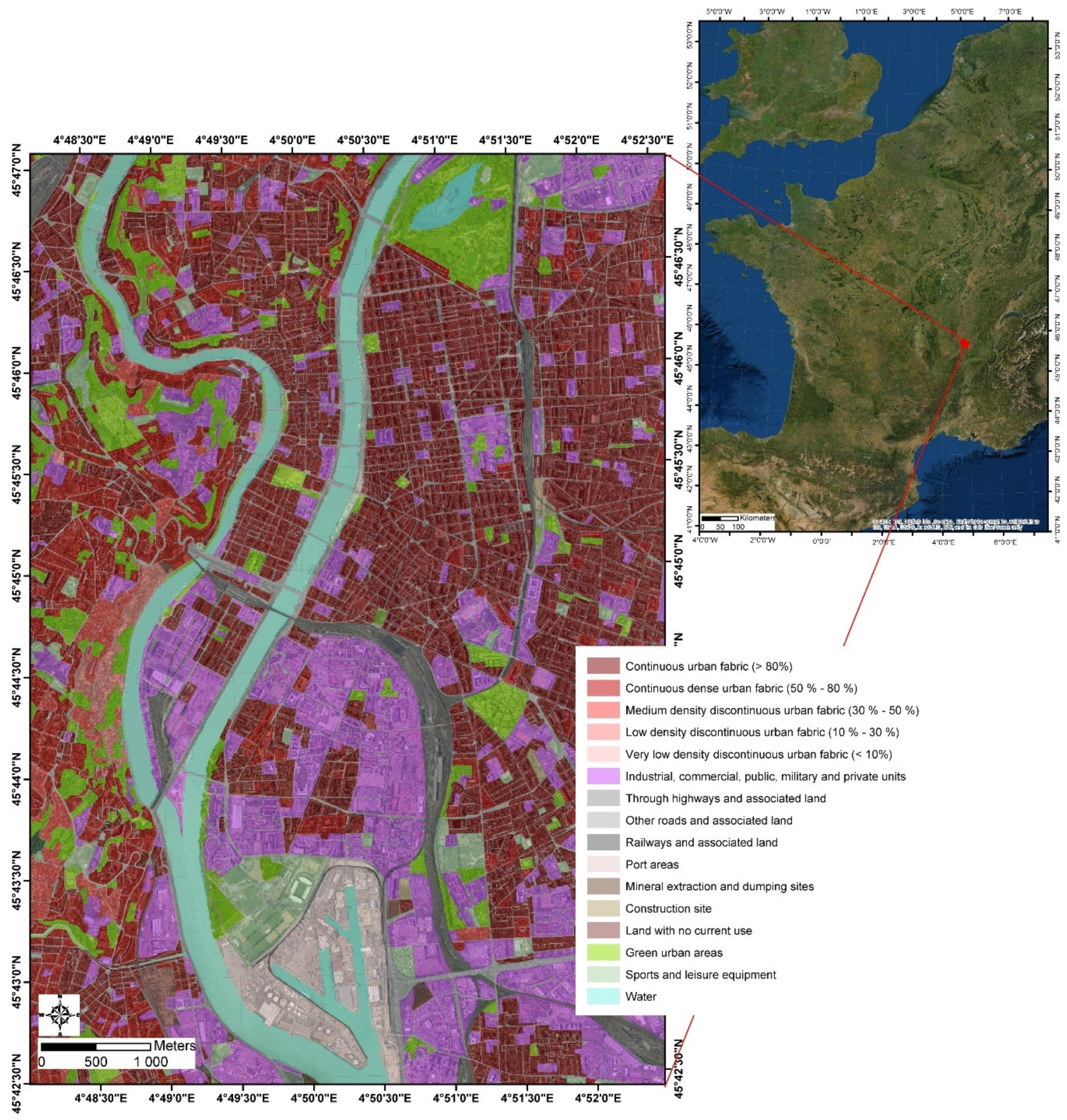
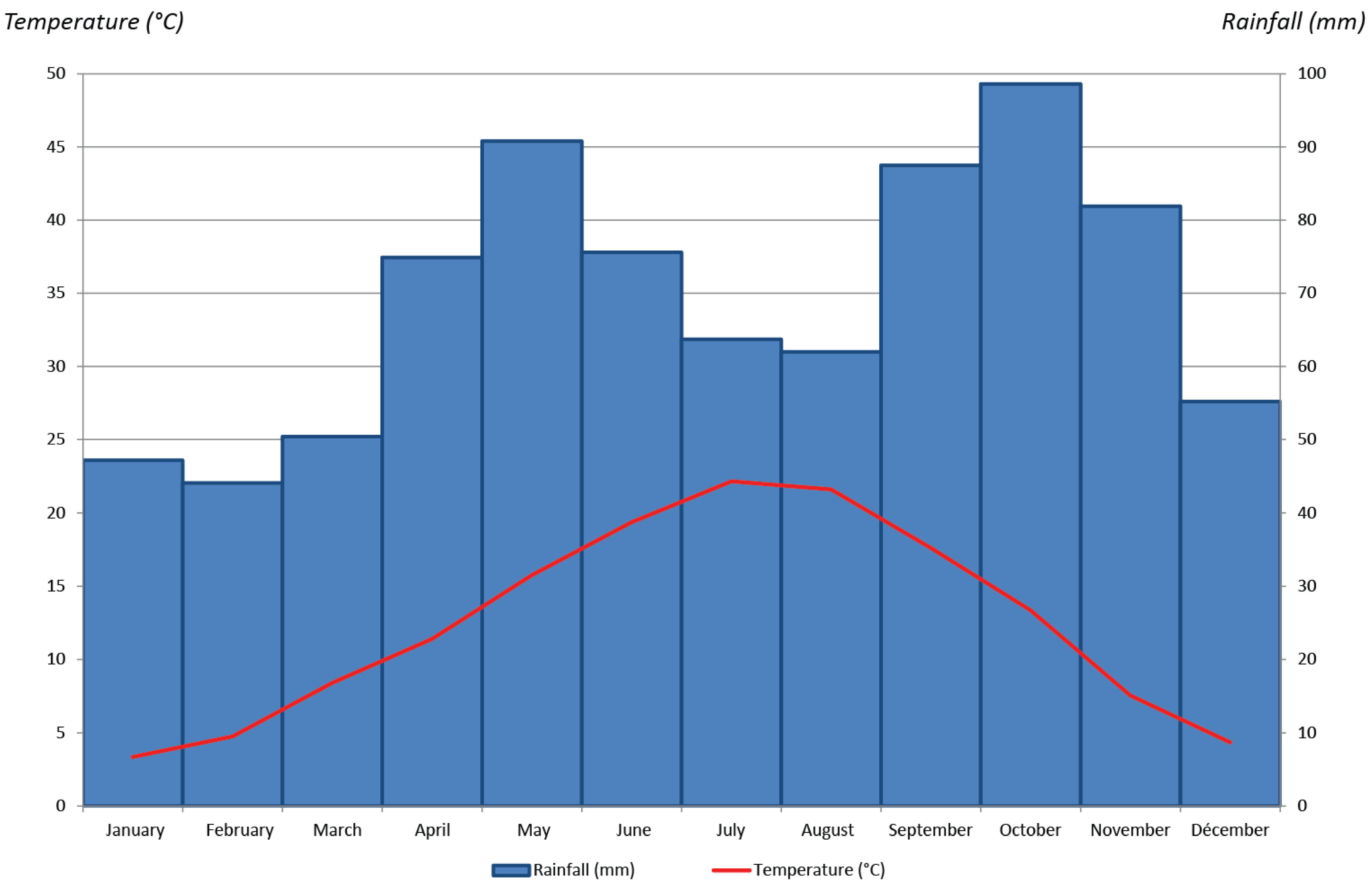
2.1. Lyon: A Study Area Characterized by a Considerable Urban Morphological Diversity

The area of interest chosen for this study is the urban heart of the city of Lyon and part of the city of Villeurbanne, on the border with the 6th district of Lyon (Figure 1). This area has the advantage of grouping together a significant diversity of land use in an urban environment. It is mainly occupied by continuous urban fabric (50%) of which 12.3% is discontinuous dense urban fabric, as well as by industrial, commercial, military, or public units (19.5%). Water, roads (main and secondary), and vegetation cover also occupy a significant surface of the territory, with respectively, 7.3%, 14.3%, and 8.9% (Table 1).
With just over 1.4 million inhabitants, this agglomeration of 59 municipalities is the second largest in France after Paris. The study area is composed of a very dense urban environment (Figure 1). Natural vegetation is therefore absent. There is, however, a very large park of 117 ha and urban green areas. The main park in Lyon (the Tête d’Or Park, to the north in Figure 1) is the largest urban park in France. It has vast expanses of lawn shaded by tall trees of various species, a lake, an island, and several botanical gardens, including an alpine garden and a flower garden.
This study area is located in the south-east of France (45°45′35″N, 4°50′32″E). According to the Köppen–Geiger classification [79,80], it has a continental temperate climate, fully humid with hot or warm summer, depending on the year (Figure 2). The hottest months are July and August, with average maximum temperatures of 27.7 °C and 27.2 °C, respectively. The wettest months are May and October with 90.8 mm and 98.6 mm, respectively. The sunniest months are June, July, and August with 254.3 h, 283 h and 252.7 h, respectively (Figure 2).

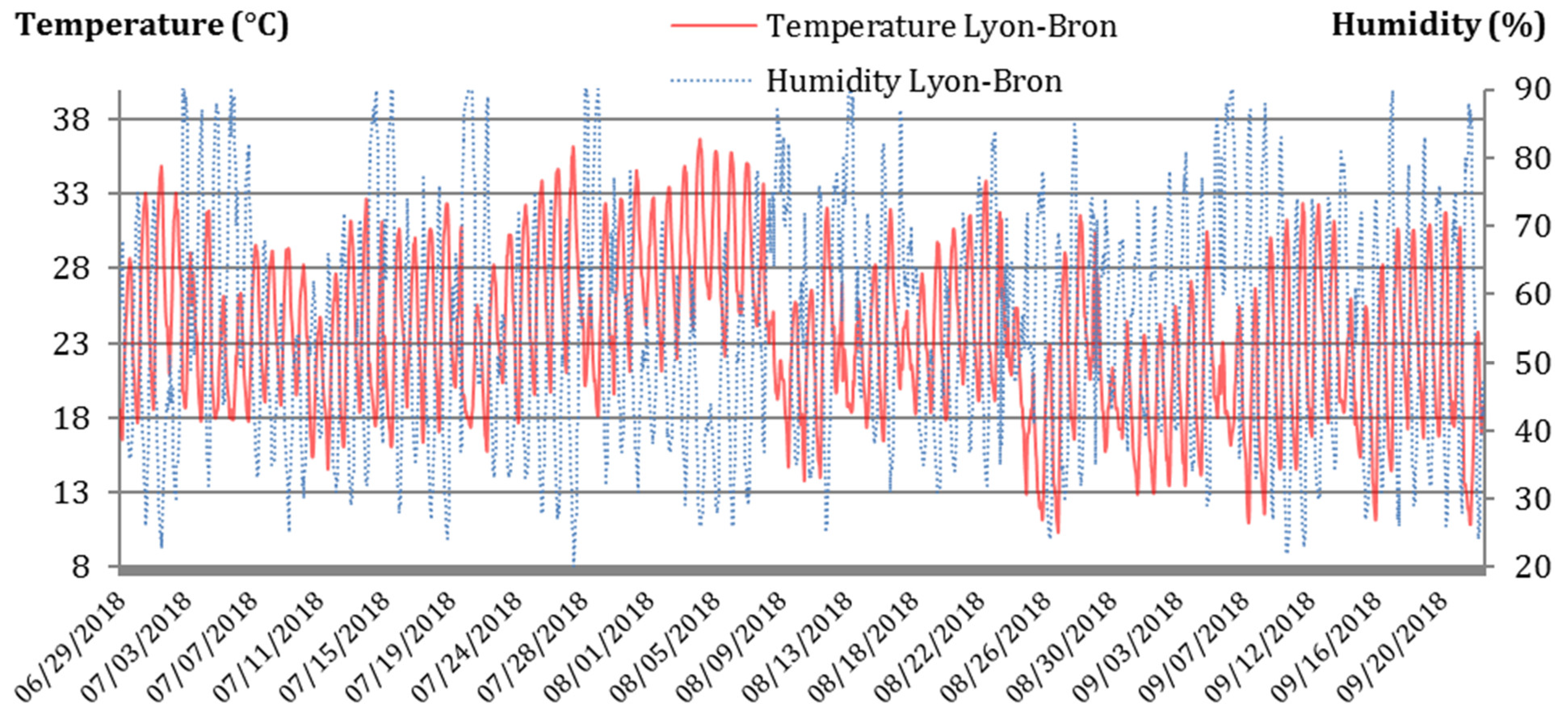
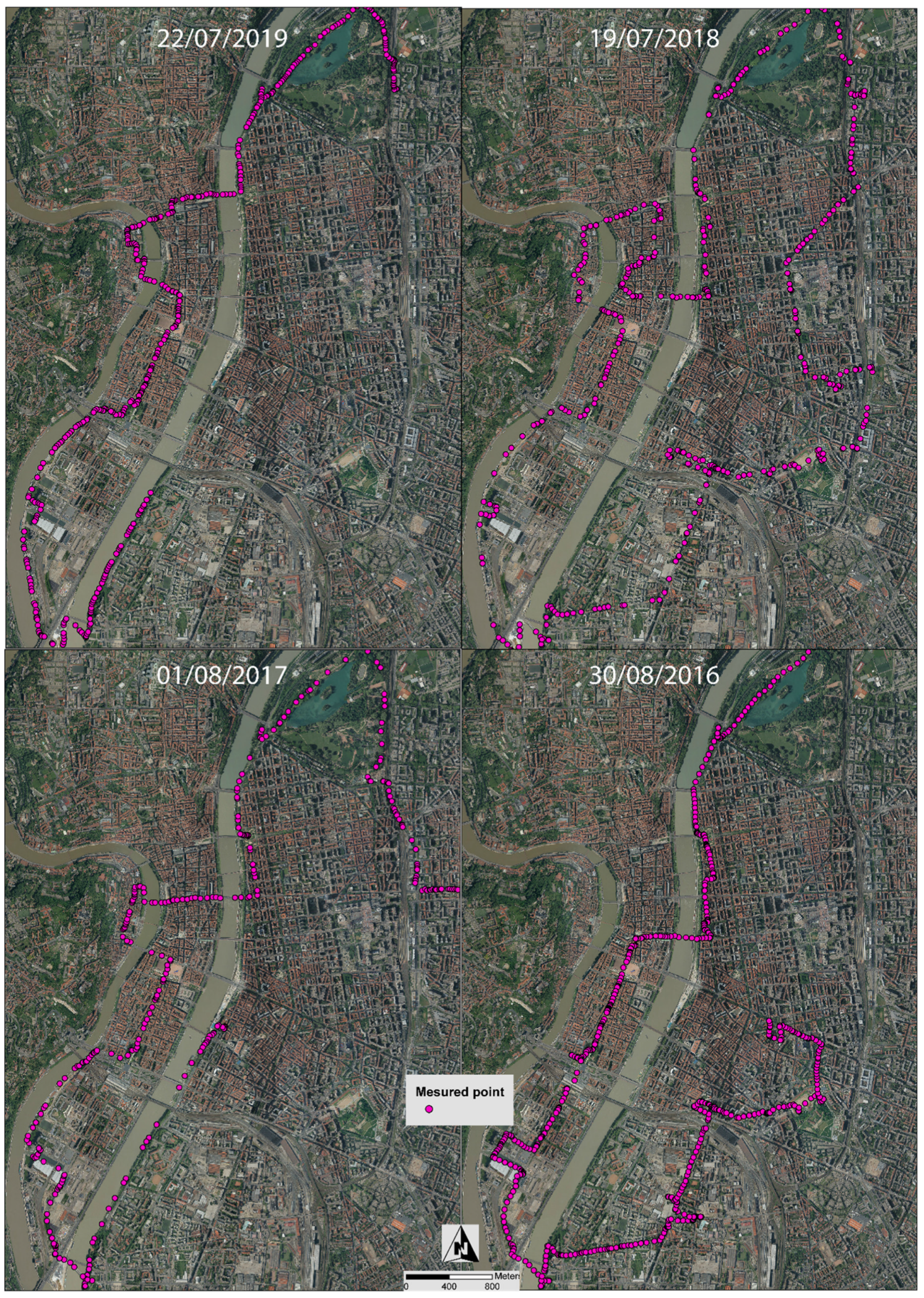
2.2. Data Acquired by the Measuring Instruments and Selected Days

Air temperature is the variable to be estimated at any point in the territory from several indicators. The training sample of this variable is obtained from mobile measurement transects using high-precision measuring devices, according to manufacturer’s data. The first equipment used is the EL-USB-1-RGC (EasyLog From Lascar Electronic). It measures the air temperature continuously, with an accuracy of +/− 1 °C (manufacturer’s data) and a minimum recording interval of 1 second. The second equipment, the LOG 32 (from Dostmann electronic GmbH), records relative humidity and air temperature, with an accuracy of +/− 0.5 °C (manufacturer’s data) and +/− 3% (40 to 60%) and a minimum recording interval of 2 seconds. The measurement campaigns were associated with a precision GPS (from Garmin, with a high sensitivity GPS/GLONASS receiver and Quad Helix antenna) to record the geographical position of the measurement.
The location of the points of all measurement campaigns was checked and corrected if necessary, using a geographic information system (GIS), for example, to ensure that it was not located on the roof of a building. Indeed, the dense urban environment can interfere with the geolocation of the position. Streets in dense urban centers may be boxed in, with little visible sky.
In addition, the Météo-France site of the Direction Centre-Est (DIRCE) of Lyon-Bron, (45°43′30″N, 4°56′12″E and 197 m altitude), was used as a study site for a quality control campaign of the air temperature and relative humidity measuring instruments. This station was chosen because it is Météo-France’s professional weather station closest to our measurement campaigns. Hourly measurements synchronous to the measurements of the Météo-France station were carried out from 28 June 2018 at 09:00 to 24 September 2018 at 14:00 (Figure 3). The comparison between site observation and mobile measurements have been done at the same time, on a single second during the exact precise hour.
The measuring devices used in this study proved to be highly accurate since, after this comparison at the Météo-France site over the summer 2018 period, the air temperature correlation of these two different acquisition sources shows a lowest correlation coefficient of 0.981 for the air temperature and 0.977 for the relative humidity measured by LOG 32 (Table 2).
The mobile measurements were taken on days when the Landsat 8 satellite was over the city, on clear sky days only, i.e., with less than 10% cloud cover. These campaigns were spread out between 2016 and 2018, exclusively over the summer period: 30 August 2016, 1 August 2017, 19 July 2018, and 22 July 2019. Numerous measurement campaigns were carried out from 2016 to 2019 but only those four days with similar weather conditions were used in this study. However, not all of them had similar weather conditions. Moreover, in only one summer of a year, the set of days was too poor regarding the different cumulative criteria, i.e., similar weather conditions and no clouds. Indeed, the weather conditions for each day were similar: the standard deviation of the temperature was only 0.9 °C and 4.3%, for humidity, 2.3 m.s-1 for wind speed, 132 degrees for wind direction, and 3.7 hPa for pressure. The average weather conditions for these indicators are 29.3 °C, 45.3%, 8.8 m.s-1, 260.8 degrees, and 1016.6 hPa, respectively (Table 3). Respectively, these measurement campaigns yielded 573, 300, 393, and 397 measurement points for air temperature and relative humidity (Figure 4).
The routes travelled during the measurement campaigns vary slightly (Figure 4). In fact, besides the technical reasons such as works or new developments that caused us to deviate from the route, we wanted to maximize the morphological diversities crossed, making deviations to places of particular interest due to their urbanistic characteristics (docks, the historic urban center, industrial sectors, etc.).
Additionally, air temperature measurement campaigns sometimes last several tens of minutes. It was therefore necessary to make a correction based on a polynomial equation elaborated according to the evolution of the day’s temperatures recorded at a time step of 10 minutes. This phase before the data processing is essential and allows to bring all these air temperature measurements back to the hottest hour of the day [74].
In addition, in order to have a very complete sample of temperature measurements, all the data from the four field trips were pooled. This allows obtaining global results. Indeed, even if the weather conditions are similar for the four days studied, some results may differ due to the different routes carried out, which cross different urban morphologies. For example, in Lyon, the type of buildings and the urban morphology are relatively different depending on whether one is in the east, with modern buildings from the end of the 19th and 20th centuries, or in the west of the main river, with very old buildings from the medieval or Renaissance period (Figure 1 and Figure 4). This could explain why the results between the days of 2019 and 2018, for example, were not strictly identical, although general trends may emerge.

2.3. Morphological Descriptors Relevant to Air Temperature Estimation

Changes in land-use patterns related to the urban factory contribute to the spatial structuring of the urban landscape, which also influence energy transmission and balance [81,82]. These changes are considered a direct cause of the formation of the UHIs [83,84]. Thus, the relationship of changes in air temperature to land use and land cover is apparent.
In this study, thirty-eight explanatory variables contributed to the estimation of air temperature over the study area [85,86,87,88,89]. They belong to various categories such as climate data from remote sensing, topographic variables, vegetation indices, the presence of water, moisture, bare soil, buildings, radiation, urban morphology, and proximity to various land uses (Table 4 and Appendix A). The acquisition sources were multiple and came from the Landsat 8 satellite (https://earthexplorer.usgs.gov/), LiDAR (https://data.grandlyon.com/jeux-de-donnees/nuage-points-lidar-2018-metropole-lyon-format-laz/donnees) points and other cartographic products downloaded from the open data platform of the Greater Lyon.
These morphological descriptors are acquired to a spatial precision that can go down to the centimeter scale. As a result, the information collected is dense and allows us to acquire a rigorous state of the urban environment for the purpose of modelling air temperature.

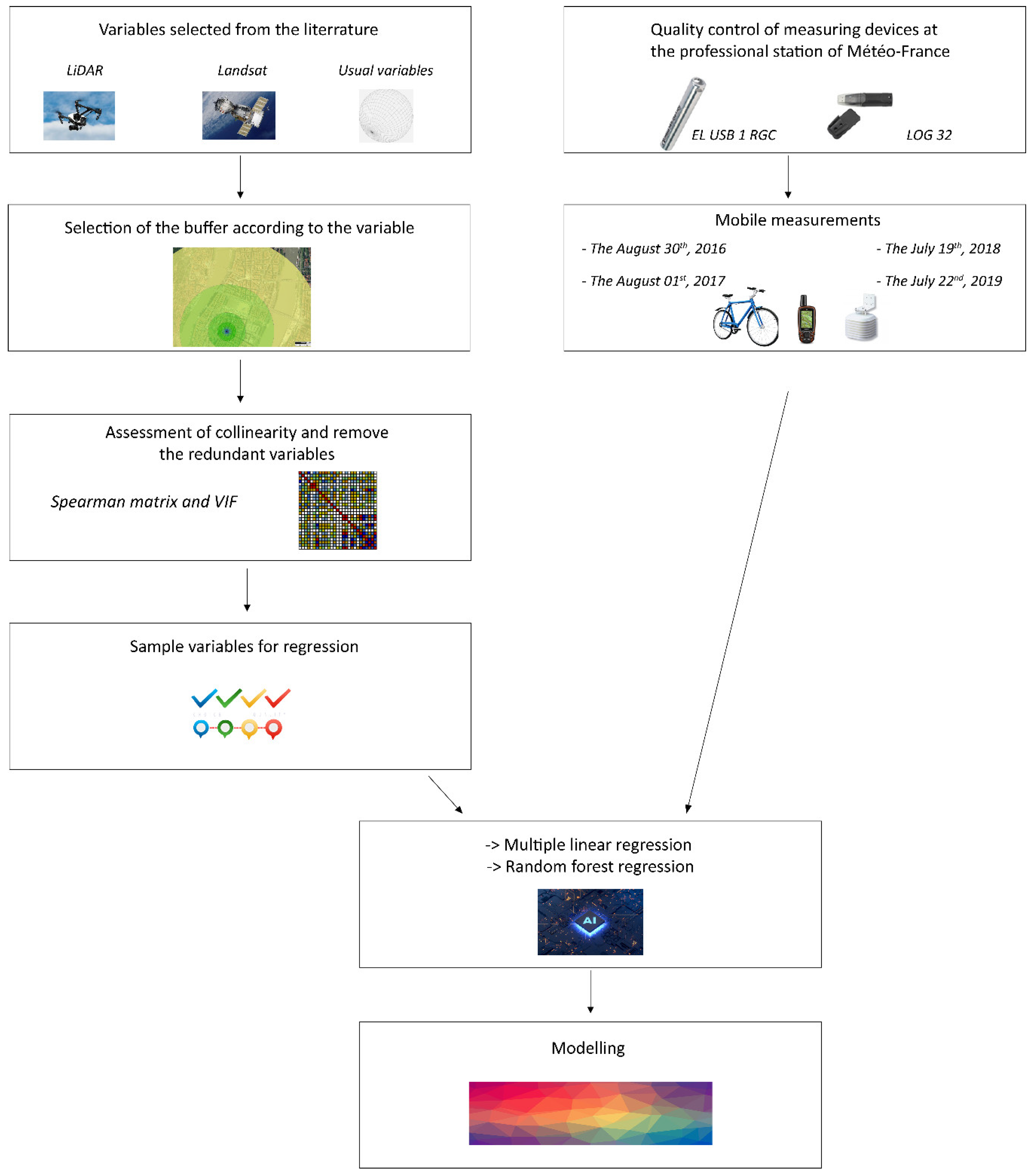
2.4. The Statistical Procedure Followed

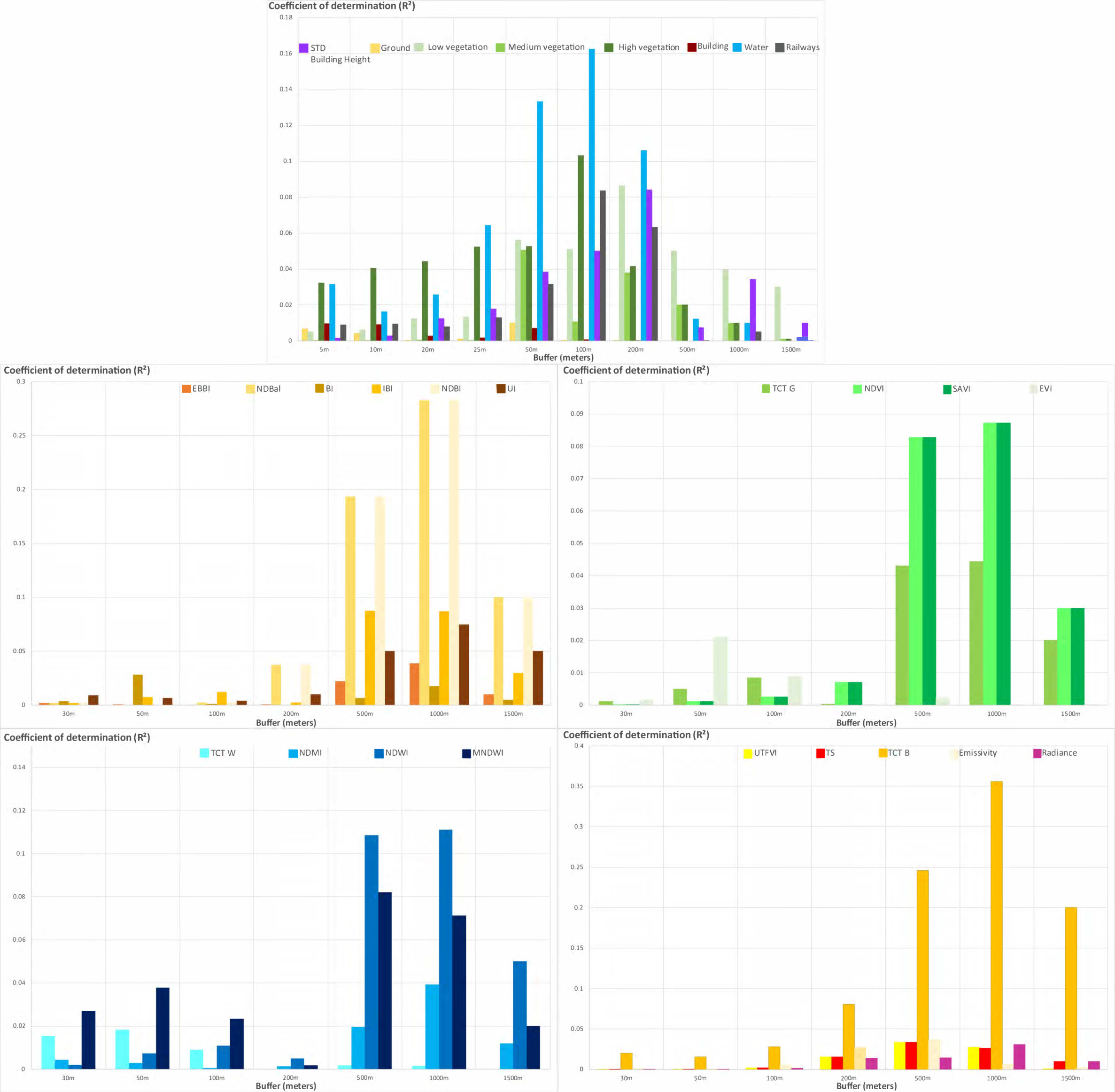
2.4.1. An Explanatory Buffer Zone, Which Varies According to the Indicator

The aim of this study is to model air temperature using the linear regressions, multiple and partial least square regressions, and nonlinear regression by the random forest regression, from selected predictors. Initially, the scale with the best correlation between air temperature and explanatory variables was selected for each indicator based on a proximity buffer analysis (5 to 1000 m; Figure 5). Thus, the selected buffer zone varies for indicators of the presence of vegetation, water, humidity, bare soil and buildings, radiation indices, proximity to land use, urban morphology, and finally climate data (Table 5). Each of the measuring points was compared with the average of the indicator concerned, according to the size of the buffer considered.
For example, the process followed for the 5-meter buffer is as follows: 1°/creation of a 5-meter buffer around each point; 2°/calculation of the area (for vegetation, water surfaces, etc.), length (railways), average (spectral indices), or standard deviation (STD Building Height) of the indicator in this buffer; 3°/calculation of the Spearman correlation coefficient between the temperature measured at the point and the indicator; and 4°/repeat the operation for all the indicators and for all the buffers.

2.4.2. Three Complementary Regression Methods in Modelling Use

Three regression methods of air temperature modelling are compared in this study. These are two linear regressions: multiple [42,50,56] and partial least square [90], and one non-linear regression: random forest [91,92]. The aim is to select the best regression for this modelling. This evaluation is essentially carried out by comparing the coefficients of determination and the roots of the root mean square error (RMSE) obtained for the samples. The conditions of use for each of the regressions were also verified.
Multiple linear regression (MLR) is a data modelling method that requires several statistical steps before its application [93]. First, it is necessary to verify the normal distribution of the series in the dataset using the Shapiro–Wilk test (applies to samples of less than 5000 observations) [94]. This test has been invalidated, so the Spearman correlation matrix was used. It allows redundant variables not to be included in the regression model. One of the two indicators for which the pair has |r|>0.7 in the Spearman correlation matrix and a Variance Inflation Factor (VIF) > 5 was removed [95,96]. Finally, after removing the correlated variables, multiple linear regressions are carried out on about 20 variables, between 21 for the 30 August 2016, and 27 for the 1 August 2017 (Table 6).In addition, a holdout cross-validation was performed because of its ability to detect multiple regression overfitting (80% learning data and 20% validation data) [97].
In a complementary way to the multiple linear regression (MLR), partial least square regression is a method that is applied when a large number of explanatory variables are present and when these variables are likely to show strong collinearities among themselves [98]. Thus, this method allows us to model and predict air temperature values as a function of a linear combination of several quantitative (or qualitative) explanatory variables, overcoming the constraints of linear regression with respect to the distribution and number of variables included. Therefore, there is no need to remove the collinear variables. The model gives a value for each Variable Importance for the Projection (VIP). An explanatory variable is considered important when the VIP is greater than 0.8 [99]. A standardized coefficient is then generated for each of them [100].
The third type of regression tested is the random forest regression. This is a predictive model using binary decision trees [101]. From an observation sample, the bagging method will generate several possibilities before selecting only one. This machine learning technique [102] is based on Classification and Regression Trees (CART). These are constructed from different bootstrap samples, randomly selected with random discounting, in order to obtain, after aggregation, a robust and efficient set of air temperature predictors [103]. The importance of each variable is calculated by the mean increase in error of a tree in the forest, i.e., when the values of each variable are randomly swapped in the out-of-bag (OOB) samples. The variables used in the nonlinear regression, random forest, to model air temperature are derived from the selection of multiple linear regressions for each day. The random t forest classification and regression has the advantage of reducing white noise, and thus potentially improving the correlation coefficients and RMSE already obtained by multiple linear regression. In addition, the number of variables in the bagging and the number of trees used are user-defined parameters. When the number of trees increases, the general error converges to the same value. Overfitting is then not a problem due to the large numbers law. Despite this, the number of analysed trees must be limited in order not to excessively increase the computation time (1):
c × T × v × ( M × N × log N )
where c is a constant, T is the number of trees in the set, M is the number of variables, and N is the number of samples in the training data set [104]. In this work, the classifiers were optimized with 80 decision trees and were trained with the same number of pixels in each category. The general error of the models converged around 80 decision trees (Figure 6). Therefore, a more complex model would have required more computation time without improving the classification.
In addition, Lasso regression was not applicable in this study. Lasso regression is only used when the number of predictors is greater than the number of observations [105,106]. Here, though, the number of observations was much higher than the number of predictors. In addition, many explanatory variables were included.

2.4.3. Quality Control on Modeling by Spatial Identification of Error Clusters

The spatial autocorrelation of the difference between the modelled air temperature and the air temperature measured by the mobile measurements was analyzed, on one hand, using the Anselin Local Moran I spatial association indicator (LISA) [107], and, on the other hand, using the degree of clustering of high and low intensity values by the Getis Ord General G (Gi*) [108,109].
The LISA makes it possible to group together, for statistically significant results (p < 0.05), the similarity of a spatial unit with its neighbours. It allows identifying spatial aggregates of entities with high or low values as well as spatial outliers. A cartographic representation showing a cluster type for each statistically significant entity is thus obtained. With a geographic information system (GIS), a statistically significant group of high values (HH), a group of low values (LL), an outlier in which a high value is surrounded mainly by low values (HL), and an outlier in which a low value is surrounded mainly by high values (LH) is distinguished.
The local application of the general G statistic is the Getis Ord Gi* statistic. It is used to identify statistically significant (p < 0.05) spatial clusters of high and low intensity. Thus, for positive Z scores, the higher the Z score, the stronger the cluster of high intensity values (error overestimating air temperature). On the contrary, the lower the negative Z-score, the higher the group of low intensity values (error underestimating the air temperature).
In order to summarize the methodology, a general diagram of the study has been inserted (Figure 7).

3. Results

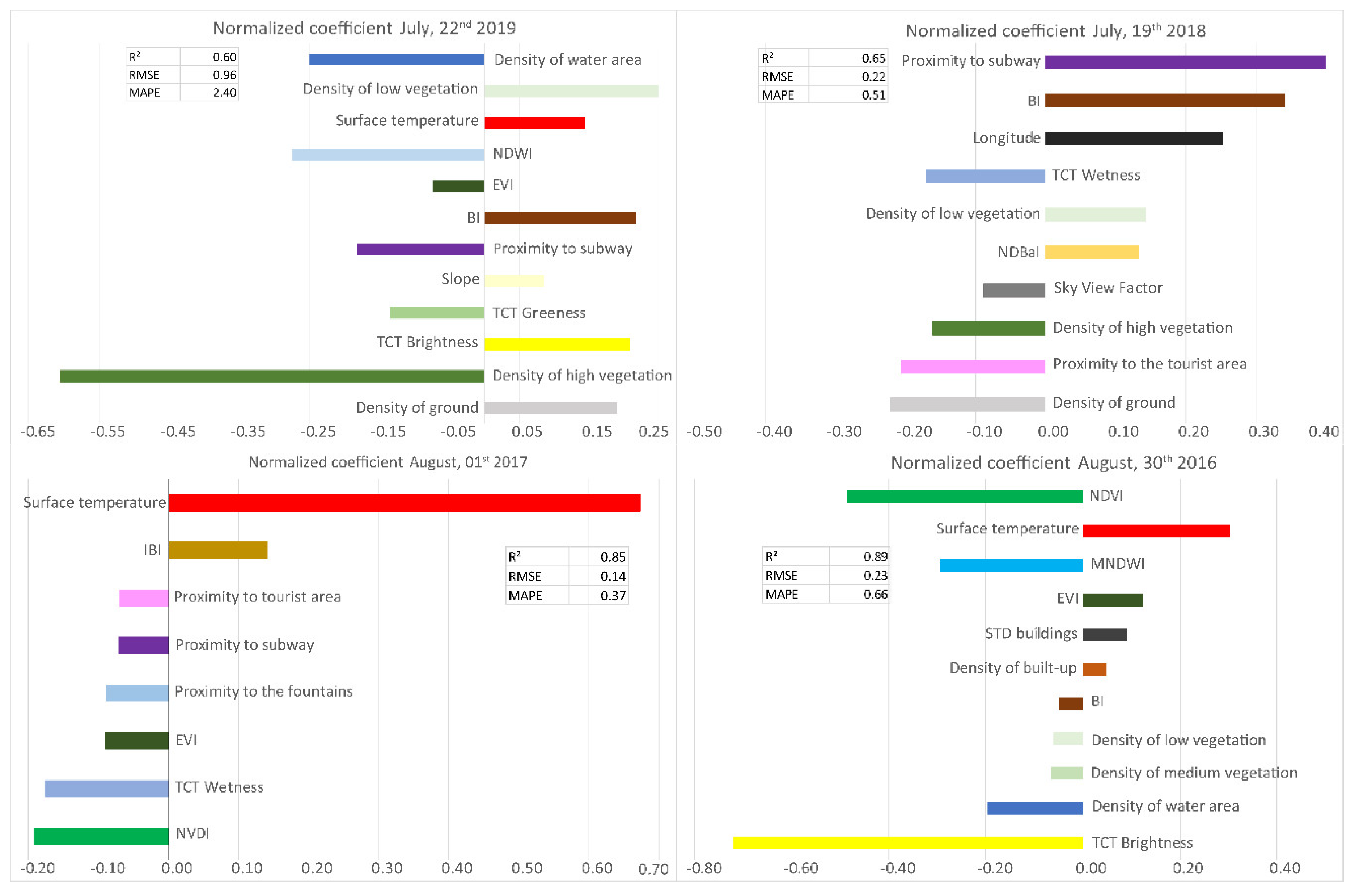
3.1. Multiple Linear Regression Modeling

After removing the collinear variables for each day, the predictors involved in air temperature modelling provide significant coefficients of determination. These ranged from 0.60 for 22 July 2019, to 0.89 for 30 August 2016, with RMSEs of only 0.96 °C and 0.23 °C, respectively. Moreover, each variable retained in the model was characterized by a normalized coefficient that corresponded to the weight of this explanatory variable. This weight varies according to the study days (Figure 8). The probability associated with Fisher’s F (Pr>F) was always less than 0.05 and very often less than 0.0001.
For example, for 19 July 2018, the variables contributing to a positive impact on the model were proximity to subways, Bare Soil Index (BI), longitude, Tasseled Cap Transformation (TCT) wetness, low vegetation density, and Normalized Difference Bareness Index (NDBaI). Variables negatively impacting the model are sky view factor, high vegetation density, proximity to tourist attractions, and soil density. From the equation obtained, it is therefore possible to model the air temperature continuously. The resolution can be adapted to the display and the purpose of the study. For example, a resolution of 10 meters was chosen for Figure 9 (Figure 9). It can be seen in Figure 9 that some areas are cooler or hotter than others on the map. This is directly related to the equation used in the modelling, including the explanatory variables included, as shown in Figure 8. Thus, for example, in Figure 9, cold spots at some locations are related to the density of tall vegetation or water surface. Hot spots, in contrast, would be related to low vegetation density, soil density, or BI. Thus, the greater the presence of these variables, the greater the chance of detecting a hot or cold spot. This confirms the results of previous studies showing in particular the cooling power of tall vegetation [43,110], water surfaces, or urban density [33,111,112].
The results for the sample with all measurements for the four outputs (Figure 10) show an R2 of 0.65 and an RMSE of 1.54. The results for the sample with all measurements for the four outputs (Figure 10) show an R2 of 0.65 and an RMSE of 1.54. The RMSE is logically slightly higher than for the single day models due to the larger sample of measurements and greater morphological diversity, even though the weather conditions remain similar. These results confirm the general trends observed at day scales. In particular, the cooling effect of variables such as water density (normalized coefficient of –0.35; Figure 10), densely vegetated areas (–0.11 for NDVI and –0.09 for the density of high vegetation), road embankment (–0.08 for SVF), and humidity (–0.05 for Modified Normalized Difference Water Index (MNDWI)) can be found. The presence of proximity to tourist areas can be explained by the fact that these areas are mostly made up of green spaces or historic buildings in old Lyon.
The variables contributing to urban warming were logically surface temperature and emissivity (normalized coefficients of 0.53 and 0.26, respectively; Figure 10) as well as indicators of the built environment and the absence of medium or high vegetation density (0.13 for the NDBaI, 0.12 for the Index-based Built-Up Index (IBI), and 0.23 for the density of low vegetation).

3.2. Partial Least Square Regression Modeling

Partial least square (PLS) regression modeling did not show much consistency in air temperature prediction since the mean coefficient of determination for all four study days is only 0.62, with a maximum of 0.79 for 30 August 2016, and a minimum of 0.53 for 22 July 2019 (Table 7). In addition, a large number of explanatory variables were retained, with a maximum of 26 for the day of 22 July 2019. Some variables influenced the model both positively and negatively as a function of the day. For example, the MNDWI had a significant positive impact for 30 August 2016, and a negative impact for 1 August 2017, 19 July 2018, and 22 July 2019. As a result, the air temperature modeling results were much less relevant than by multiple linear regression.
Overall PLS modelling based on the measurements of the four outputs provided results relatively similar to multiple linear regression, with an R2 equal to 0.699 and an RMSE of 1.503. They also confirmed the dominant role of surface temperature. This variable had a VIP of 2.2. This is followed by the density of water areas (VIP = 1.81), the density of low vegetation (1.43), the NDVI (1.15), and the humidity indices (1.03 for the MNDWI and 1.01 for the TCT Wetness). These results are in agreement with those obtained through multiple linear regression (Section 3.1).

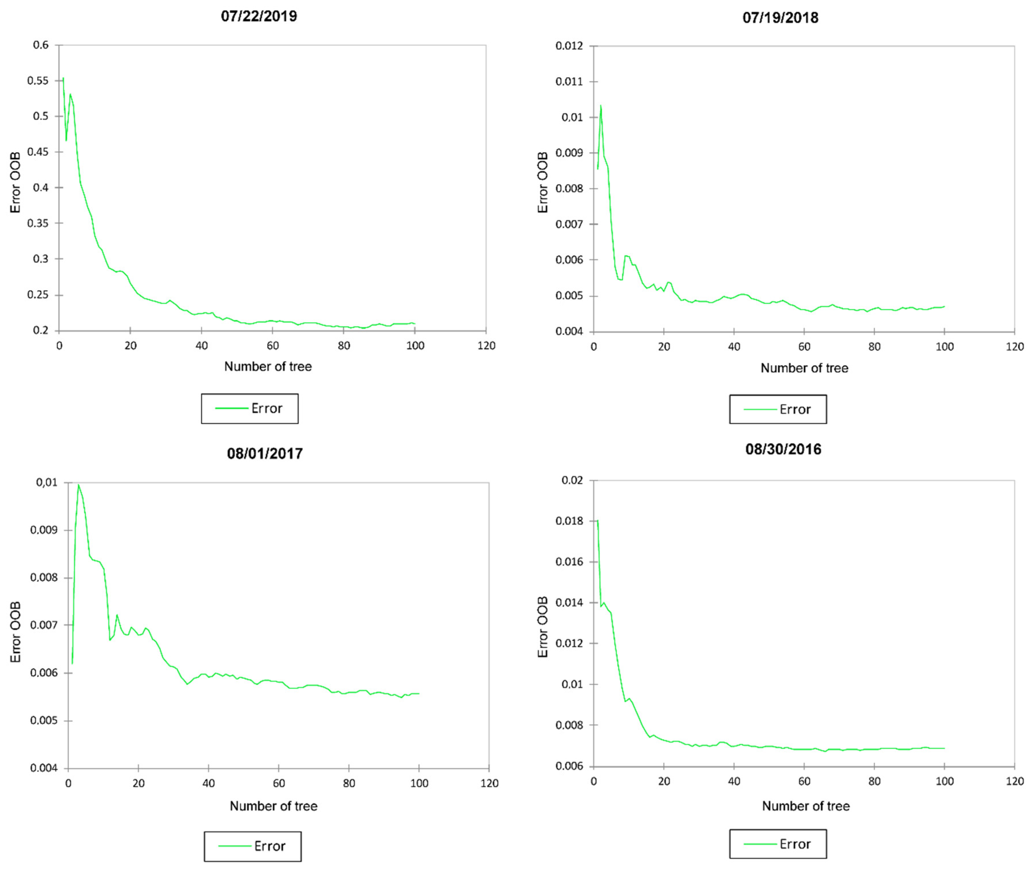
3.3. Random Forest Regression Modeling

For the four study days, the coefficients of determination obtained were strong: 0.98 for the 30 August 2016, 0.96 for the 1 August 2017, 0.95 for the 19 July 2018, and 0.92 for the 22 July 2019 (Table 8). Thus, on average, a coefficient of determination of 0.95 was obtained, with a RMSE of only 0.17 °C and an out-of-bag (OOB) error of 0.05.
In addition, the measure of importance for each of the variables was measured by the mean increase in error of a tree in the forest when the observed values of that variable were randomly swapped in the out-of-bag samples (OOB; Figure 11). As a reminder, an increase in errors allowed us to know the importance of the variable in the modeling.
Global random forest modelling based on all days highlighted the dominant role of surface temperature, which had a mean error increase of 102.5 (Figure 12). This was followed by emissivity, density of low vegetation, IBI, and density of high vegetation with mean error increases of 26.9, 23.5, 16.2, and 16.2, respectively (Figure 12). These results are in agreement with those obtained using multiple linear regression and PLS regression.

4. Discussion

4.1. Implication of Important Predictors in Urban Air Temperature Modeling

The results of the simple regressions (Section 2.4.1 and Figure 4), the multiple linear regression (Section 3.1), the Random forest regression (Section 3.3), and to a lesser extent the PLS regression (Section 3.2) make it possible to identify the parameters that positively and negatively influence urban air temperature. Naturally, surface temperature is frequently used in air temperature modelling (22 July 2019; 1 August 2017; and 30 August 2016; Figure 8) with very high weights (normalized coefficient of 0.67 for the day of 1 August 2017; Figure 8), mean error increase of 59.2 and 48.1 for the days of 30 August 2016, and 1 August 2017, respectively (Figure 11, for example). This is confirmed by the overall results of multiple linear regression and random forest modelling. Its normalized coefficient is 0.53 and its mean error increase is 102.5. However, this is not an urban morphological descriptor on which designers, urban planners, or politicians can directly act. The urban parameters highlighted by the models that can be influenced in planning operations to combat extreme temperatures in cities mainly concern green and blue solutions, and grey solutions [113,114,115].
Modelling results indicate that the factors that contribute to increasing temperatures in urban areas are related to building density. Indeed, regarding the density of buildings, for example, the BI had a normalized coefficient of 0.22 on 22 July 2019, and 0.34 on 19 July 2018. The TCT Brightness, which refers to bare, partially covered or waterproofed soils (such as rocky outcrops, concrete, gravel, asphalt, etc.) had a normalized coefficient of 0.21 for 22 July 2019, and a mean error increase of 31.5 for 30 August 2016, and 8.4 for 22 July 2019. The IBI had a coefficient of 0.14 and a mean error increase of 30.5 for 1 August 2017. To a lesser extent, we also found the presence of low vegetation (and thus the absence of high vegetation), which had normalized coefficients of 0.22 and 0.15 for the days of 22 July 2019 and 19 July 2018, respectively, and mean error increases of 15 and 35 for 30 August 2016, and 19 July 2018, respectively. This was confirmed by the overall results of multiple linear regression and random forest modelling. Its normalized coefficient was 0.23 and its mean error increase is 23.5 (Figure 10 and Figure 12).
By contrast, the factors that favor the decrease in urban temperatures were related to the presence of vegetation, humidity, and surface water. Thus, high vegetation density had a high cooling power in the models with normalized coefficients of −0.6 for 22 July 2019 and −0.15 for 19 July 2018, and a mean error increase of 19 for 22 July 2019. These results are consistent with those of the global modelling using multiple linear regression and random forest. Its normalized coefficient is −0.09 and its mean error increase is 16.2 (Figure 10 and Figure 12).
In addition, NDVI was found with normalized coefficients of −0.5, −0.18, and −0.11 and mean error increases of 20, 8, and 7.6 for the days of 2016, 2017, and globally, respectively, but also TCT greenness (−0.14 for 22 July 2019). Moisture also had a cooling effect through the TCT wetness (with normalized coefficients of −0.18 and −0.17 and mean error of 6 for 1 August 2017, and 19 July 2018, respectively) or proximity to fountains (with normalized coefficient of −0.09 and mean error of 10.4 for 1 August 2017). Finally, the density of water area has a negative impact on the model with normalized coefficients of −0.29, −0.20, and −0.35, and mean error increases of 18.9, 41.4, and 10.7, respectively, for 22 July 2019, 30 August 2016, and in a global way, as well as the NDWI (with a normalized coefficient of −0.27 and mean error of 11.7 for 22 July 2019) or the MNDWI (with respectively for 30 August 2016, and 19 July 2018, a mean error of 19 and 48.6).
To our knowledge, this is one of the studies aimed at modelling air temperature in a morphologically contrasting urban environment, with areas of unequally dense habitat, two rivers, a historic center and the largest urban park in France (Figure 1), which uses the most extensive sample of explanatory variables, with classic data, LiDAR data, and data from remote sensing. This study has shown the interest of the complementary use of the latter two types of data, in particular LiDAR for a precise view of vegetation densities (high, medium, or low) but also remote sensing for surface temperature and water, humidity, and vegetation indices to a lesser extent. While we expected very satisfactory results with random forest modelling, confirming the results of previous studies [63,97,116], we were surprised to note also the very high performance of the classical multiple linear regression and PLS regression, with very low RMSE and often below 0.5 °C.
These results confirm the roles played by vegetated spaces [43,110], building density, and water surfaces in previous studies [33,111,112] and confirm mitigation practices based on green and blue space solutions [113]. This study also highlighted the relatively low cooling power of low vegetation during the sunny afternoons of the measurement campaigns. Even if we had observed this during the measurement campaigns, this had yet to be confirmed by the models. This weakness can be explained by the density of vegetation, which is not high enough to promote sufficient evapotranspiration for cooling, but above all by a lack of shade compared to the tall vegetation.
Finally, the influence of buildings on air temperature is generally considered within a radius of 500 m [117,118,119,120]. However, in this study, it was found that the buffers with the best correlation between air temperature and building density, based on LiDAR data, were 5 and 10 m. Furthermore, the vegetation density obtained from LiDAR, which explains air temperature in an optimum way, was within a radius of 50 to 200 m, regardless of its height (low, medium, or high; Figure 5). This also corresponds to a smaller buffer size than that used in previous studies [46]. On the other hand, the buffer size for the bare-soil surfaces was between 50 m and 1000 m depending on the indicator (respectively density of bare-soil and BI, and NDBaI, and Enhanced Built-Up and Bareness Index (EBBI)). In this latter case, this size is similar to that of previous studies [46].
Consequently, this methodology based on mobile cycling measures, buffer analysis and regressions using complementary explanatory variables are fully applicable to other cities. However, we recommend testing the choice of scales for these variables, all the more so if it is not an old European city with morphological urban similarities to Lyon, although the optimal radii found in this study coincide with previous similar experiences in other cities.
In addition, it can be noted that similar spectral indices significantly correlate with the air temperature at the same scale because of the similar physical meaning represented by the indices. For example, vegetation indices such as TCT greenness, NDVI, and Soil Adjusted Vegetation Index (SAVI) are most relevant between 500 and 1000 m, as are water indices (NDWI or MNDWI), building indices (NDBI and Urban Index UI) and bare soil indices (NDBaI and TCT Brightness).

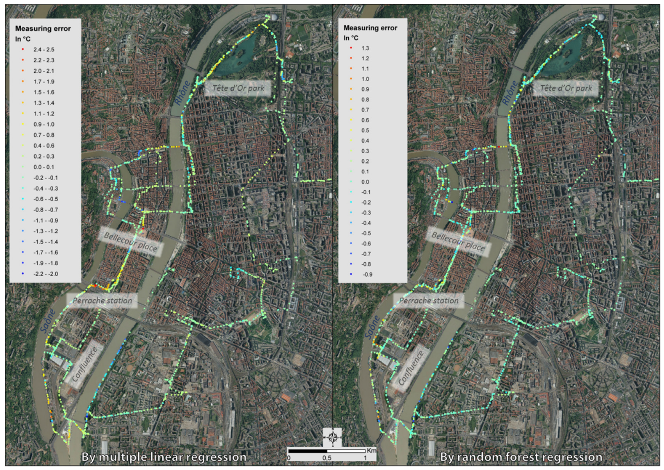
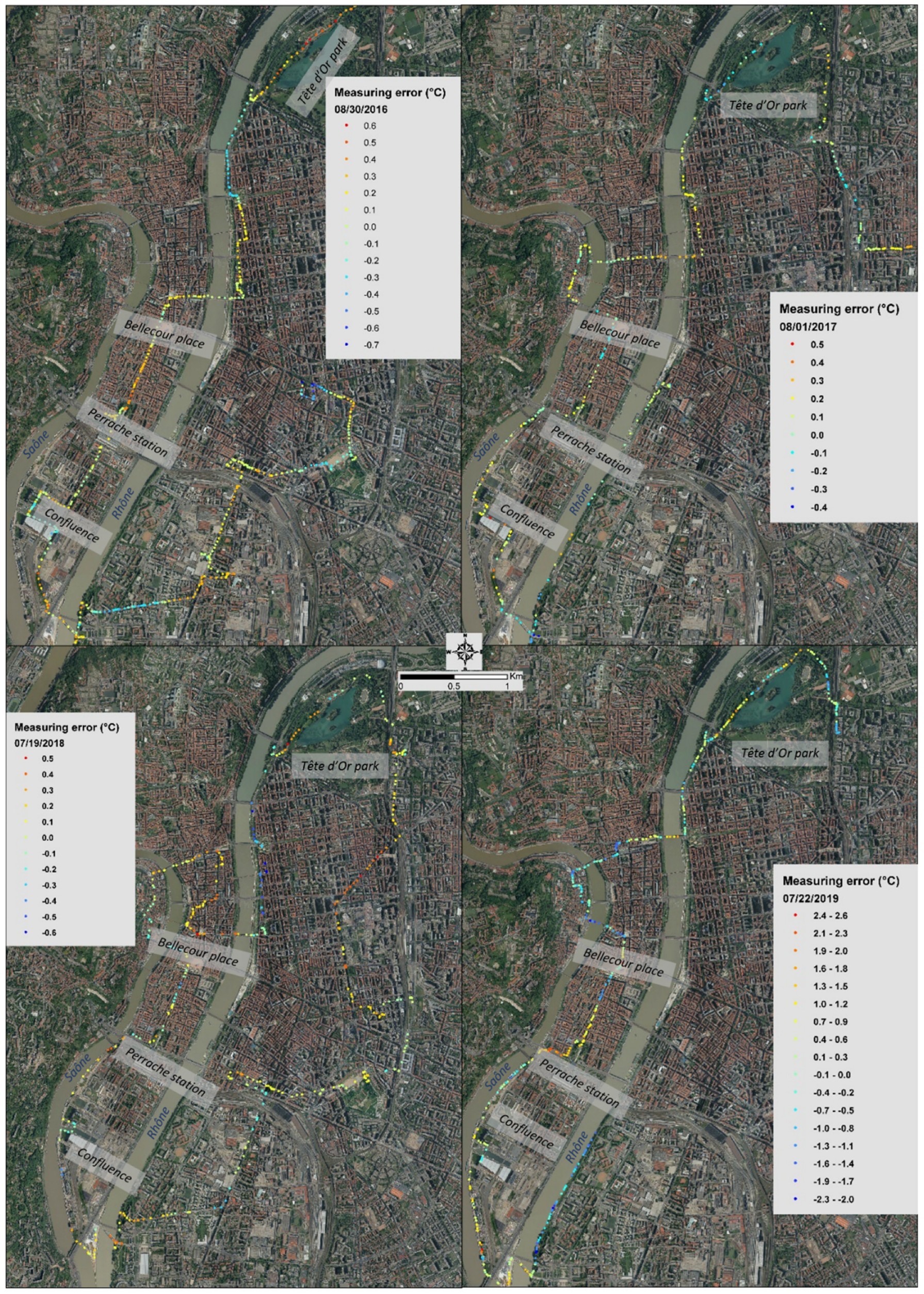
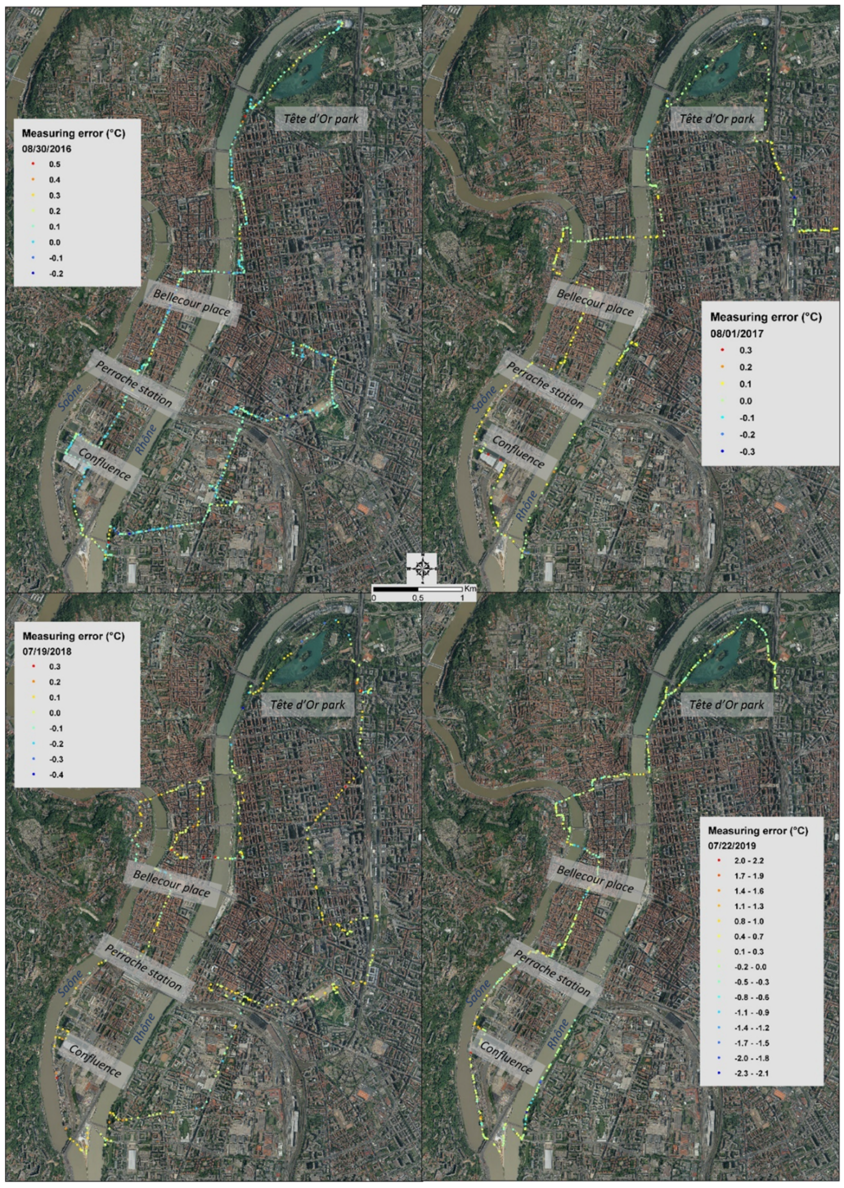
4.2. Spatialization of Error

The modelling error found is minimal for multiple linear regression and random forest modelling. For all study days, the median for multiple linear regression modelling was 0.02 °C and for random forest classification and regression modelling was 0.002 °C (σ of 0.44 and 0.17, respectively; Table 9). In contrast to the closeness of the median and mean values by these two modelling methods, the agreement is stronger for multiple linear regression than for random classification and regression forest (Figure 13).
When looking at the location of errors in air temperature modelling between the multiple linear regression method and the random forest, similarities between the two are observed. The models overestimate the air temperatures towards the water areas on Confluence (south of the peninsula) and near the Perrache train station. They underestimate the air temperature in the streets in the embankment, near green areas, and south of the left bank of the Rhône (Figure 14).
If we analyze the location of these errors day by day, we notice that for the 30 August 2016, the multiple linear regression model overestimates the air temperatures near the water areas, on the bridges and south of the left bank of the Rhône. Conversely, it underestimates this physical magnitude on open spaces such as Bellecour Place. For 1 August 2017, 19 July 2018, and 22 July 2019, the model overestimates the air temperature also near the waterways and on the bridges but also on open spaces. In contrast, the model suggests that the streets in the embankments are cooler than in the mobile in situ measurements (Figure 15). The same can be seen in the random forest modelling (Figure 16). In addition, an overestimation of air temperature near the green spaces of the Tête d’Or Park was observed for the days of 30 August 2016, 19 July 2018, and 22 July 2019.

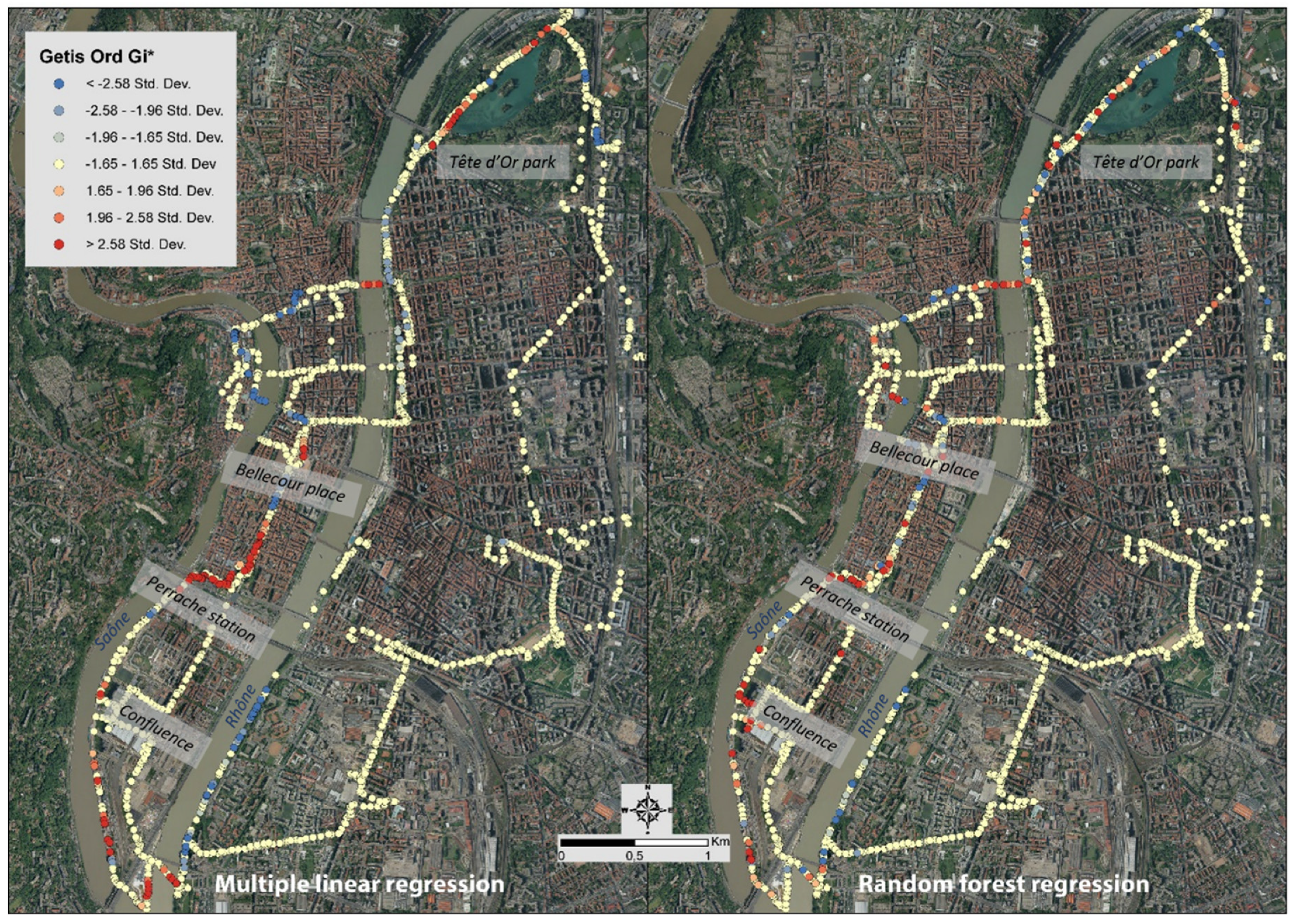
4.3. Grouping of Similar Errors

Spatial groupings of statistically similar values of the differences between modelled and measured air temperatures are evaluated using LISA (Figure 17) and Gi* (Figure 18). Between the two regression methods (linear multiple and random forest), similarities in the location of error clustering types by LISA and Gi* are observed. As a reminder, for LISA, the distinction is made between a statistically significant cluster consisting of high values only (HH), a cluster of low values only (LL), a cluster in which a high value is surrounded mainly by low values (HL), and a cluster in which a low value is surrounded mainly by high values (LH).
Firstly, using the LISA method, clusters of small errors (LH), underestimation of the model in relation to the measured values, can be identified on the left bank of the Rhône, in the steep streets of the peninsula and Vieux Lyon district, and on bridges. Areas with a high value (HL), i.e., an overestimation of the model, can be observed near the Perrache train station, in the Confluence area, and near the green spaces of the Tête d’Or park (Figure 17).
Secondly, groupings of the errors of underestimation and overestimation of the air temperature modelling compared to that measured by the Gi* method are located in areas similar to the LISA. These recurring areas for statistically low negative z-score values are the steep streets of the peninsula and Old Lyon and the south of the left bank of the Rhône. The statistically high positive z-score values are the Perrache train station and Confluence district, the proximity to the green spaces of the Tête d’Or park and the Morand bridge (Figure 18).

4.4. Limits and Future Research Outlooks

When looking at the positive or negative effects of variables on air temperature, it can be noticed that some can vary depending on the day being studied. For example, on 22 July 2019, the density of ground affects the air temperature positively, but on 19 July 2018, it had a negative impact. This is probably related to the route that differs between the two rides. The 2018 route is almost twice as long as the 2019 route (Figure 4) and the 2019 route passes through different neighborhoods, especially with regard to soil characteristics. This would indicate, among other reasons, why the results may differ depending on the days studied. In addition, the data provided by LiDAR concerning the ground is of a different nature, such as impermeable concrete or sandy soil for example, and may fluctuate depending on the routes taken. The same observation can be made for the proximity to metro stations. The proximity of the subway entrances is a variable that can affect air temperature in opposite ways. In our own experience, some subway entrances seem to give off fresh air and other entrances seem to give off warm air. When looking at the overall results of multiple linear regression modelling, it should be noted that these two variables are not included in the explanation of air temperature for these reasons.
The number of days processed for this study is one of its limitations. Indeed, only four days were analyzed. This limited number was partly due to the availability of quality (cloud-free) data from the Landsat satellite, but also due to the reduced occurrence of similar days in terms of climatic conditions. Another point of constraint is that modelling only took place in dense urban centers.
Consequently, we can argue on two perspectives: the spatial and temporal scope of this study. In the first case, it would be interesting to extend the mobile measurements in the periphery, or even in the rural areas, to be able to model the temperature in any point of the territory and compare the urban and the outskirts results. Secondly, it would be necessary to extend this analysis not only in summer, but in all seasons and at different moments of the day and at night, and for different weathers. Therefore, a global model could be built on observations from all the experimental dates rather than separating models by date.
In addition, some other data satellites may be used. For example, the use of the Sentinel 2 satellite with a 10 m resolution may help to increase the model results using sharper spectral indices, like NDVI or NDBaI.

5. Conclusions

The objective of this study was to identify the most appropriate and efficient regression to model urban air temperature based on numerous explanatory variables of various natures. The integration of these predictors in multiple regressions and machine learning method showed very satisfactory results. In addition, this methodology can be applied in other study area. The proportion of the variance explained by multiple linear regressions in air temperature modeling for each study day is globally high, with coefficients of determination ranging from 0.60 to 0.89. The results are even better when the random forest method is used. Indeed, the average coefficient of determination is 0.95 for a RMSE of only 0.17 °C and an OOB of 0.05. On the opposite, the PLS regression provides a weaker coefficient of determination for the separate days.
For all these models, there are recurring dominant variables such as NDVI or surface temperature. Consequently, the integration of satellite predictors is a definite advantage in urban microclimate modelling by linear regression model based on mobile air temperature measurements. In this study, Landsat 8 data were used, but one prospect for improvement would be to use higher resolution Sentinel data.
When we look at the overall results for all days combined, the same trends emerge. The multiple linear regression always gives very satisfactory results with an R2 of 0.65 and an RMSE of 1.54 °C, on a par with the PLS regression which shows an R2 of 0.70 and an RMSE of 1.50 °C. The global random forest modelling based on all days, however, proposes superior results with a high R2 of 0.98 and an RMSE of 0.33 °C. This modelling method is therefore the most efficient of the three tested for this study area and this sample of measurements. However, it is less accessible than the other types of multiple regressions tested and requires a greater statistical investment.
One of the strengths of this study is also the fact that it is relatively easily applicable to other areas. The equipment used for mobile measurements is not very expensive. All that is needed is a radiation shelter, a GPS, and a temperature and relative humidity recorder. All the explanatory variables used in this study, such as land use area or satellite data, are freely available. GIS and statistical processing can also be freely available if one wishes to dispense with paying software. From a practical point of view, the most complicated part of the study remains the mobile field measurements, which are very time-consuming. Indeed, they have to be synchronized with the passage of Landsat and it is necessary to have similar and favorable weather conditions, with a completely clear sky and no wind.
The results of this study confirmed the cooling roles played by green areas and water surfaces and the problems linked to building density without vegetation in the urban overheating issue. In addition, low vegetation displayed low cooling power, mainly because of an absence of shade compared to the high vegetation and the low-density vegetation providing little evapotranspiration. This highlights the real need to use green and blue spaces solutions in order to limit the UHI and improve the thermal comfort.

Author Contributions

Conceptualization, L.A. and F.R.; methodology, L.A. and F.R.; validation, L.A. and F.R.; formal analysis, L.A. and F.R.; writing—original draft preparation, L.A. and F.R.; writing—review and editing, L.A. and F.R.; supervision, L.A. and F.R.; and project administration, L.A. and F.R. All authors have read and agreed to the published version of the manuscript.

Funding

This research received no external funding.

Acknowledgments

The authors gratefully acknowledge the EROS USGS, the Lyon Metropolis and the other data platform for the useful data, free of charge. This work would not have been possible without them.

Conflicts of Interest

The authors declare no conflict of interest.

Appendix A. Explanatory Variables Selected to Estimate Fine-Scale Air Temperature

Data CategoryVariables Used for the Input (Units)Expected Effect of the Variable on the ModelCalculation MethodReference
Climatic data from remote sensingSurface temperature (°C)PositiveSingle channel algorithm [49,89,121,122]
UTFVI
Urban Thermal Field Variation Index)
Positive U T F V I = T s T m e a n T S [87,123]
Brightness temperatures (°C)Positive B r i g h t n e s s = K 2 L n ( K 1 L s + 1 ) [124,125]
Vegetation indexNDVI
Normalized Difference Vegetation Index
Negative N D V I = N I R R E D N I R + R E D [85,126,127]
SAVI
Soil Adjusted Vegetation Index
Negative S A V I = N I R R E D N I R + R E D + L × ( L + 1 ) [126]
EVI
Enhanced Vegetation Index
Negative E V I = G × N I R R E D N I R + C 1 × R E D C 2 × B L U E + L [126]
Tasseled Cap greenness or GVINegative T C T   G = B l u e   b a n d × c o e f G r + G r e e n   b a n d × c o e f G r + R e d   b a n d × c o e f G r + N e a r I n f r a r e d   b a n d × c o e f G r + S W I R 1   b a n d × c o e f G r + S W I R 2   b a n d × c o e f G r [128]
Density of low vegetationPositiveLasTool Software (LasTool: http://lastools.org/)
Vegetation quantity according to different buffer size
[46,97]
Density of medium vegetationNegativeLasTool Software
Vegetation quantity according to different buffer size
[46,97]
Density of high vegetationNegativeLasTool Software
Vegetation quantity according to different buffer size
[110]
Water presence indexNDWI
Normalized Difference Water Index
Negative N D W I = G r e e n N I R G r e e n + N I R [85,126]
MNDWI
Modified Normalized Difference Water Index
Negative M N D W I = G r e e n S W I R 1 G r e e n + S W I R 1 [126]
Moisture indexTasseled Cap WetnessNegative TCT   W =   Blue   band × coefWr    + Green   band      × coefWr + Red   band    × coefWr    + NearInfrared   band    × coefWr    + SWIR 1   band    × coefWr    + SWIR 2   band      × coefWr [128]
NDMI
Normalized Difference Moisture Index
Negative N D M I = N I R S W I R 1 N I R + S W I R 1 [86,88]
Bare soil indexNDBaI
Normalized Difference Bareness Index
Positive N D B a I = S W I R 1 T I R S S W I R 1 T I R S [85,126]
BI
Bare Soil Index
Positive B I = ( S W I R 1 + R E D ) ( N I R + B L U E ) ( S W I R 1 + R E D ) + ( N I R + B L U E ) [126]
EBBI
Enhanced Built-Up and Bareness Index
Positive E B B I = S W I R 1 N I R 10   S W I R 1 + T I R S 1 [126]
Building indexNDBI
Normalized Difference Built-Up Index
Positive N D B I = S W I R 1 N I R S W I R 1 + N I R [85,126]
UI
Urban Index
Positive U I = S W I R 2 N I R S W I R 2 + N I R [126]
IBI
Index-based Built-Up Index
Positive I B I = N D B I ( S A V I + M N D W I ) 2 N D B I + S A V I + M N D W I 2 [126]
Building densityPositiveLasTool Software
Building quantity according to different buffer size
[46,97]
TopographicSlope (%)Depending on the contextFrom the DEM (RVT 1.3 Software (RVT 1.3: https://iaps.zrc-sazu.si/en/rvt#v))[129,130]
Exposure (°N)Depending on the contextFrom the DEM (RVT 1.3 Software)[131]
CurvatureDepending on the contextFrom the DEM (RVT 1.3 Software)[132,133]
Proximity to land occupationsWater areaNegativeWater area according to different buffer size[134,135]
Distance to fountainsNegativeEuclidean distance to nearest fountain
Distance to subway entrancesDepending on the contextEuclidean distance to the nearest subway entrance
Distance to points of tourist interestNegativeEuclidean distance to the nearest tourist point
Distance to railway tracksPositiveLength of the railways according to different buffer size
Radiation indexSpectral RadianceNegative L λ = L min ( λ ) + ( L max ( λ ) L min ( λ ) ) Q d n Q m a x [136]
EmissivityNegative = L T L n T [137]
Tasseled Cap BrightnessPositive T C T   B = B l u e   b a n d × c o e f B r + G r e e n   b a n d × c o e f B r + R e d   b a n d × c o e f B r + N e a r I n f r a r e d b a n d × c o e f B r + S W I R 1   b a n d × c o e f B r + S W I R 2   b a n d × c o e f B r [128]
Urban morphologySky View FactorDepending on the contextRVT 1.3 Software[16,111,138]
Variation in building heightNegativeStandard deviation of the building height [97,116,139]

References

  1. GIEC. Rapport Spécial du GIEC Sur le Réchauffement Planétaire de 1.5 °C. Organisation Météorologique Mondiale. Available online: https://public.wmo.int/fr/ressources/bulletin/rapport-sp%C3%A9cial-du-giec-sur-le-r%C3%A9chauffement-plan%C3%A9taire-de-15-%C2%B0c (accessed on 6 January 2020).
  2. Oke, T.R. Canyon geometry and the nocturnal urban heat island: Comparison of scale model and field observations. J. Clim. 1981, 1, 237–254. [Google Scholar] [CrossRef]
  3. Weston, K.J. Boundary layer climates. Q. J. R. Meteorol. Soc. 1988, 114, 1568. [Google Scholar] [CrossRef]
  4. Oke, T. City size and the urban heat island. Atmos. Environ. 1973, 7, 769–779. [Google Scholar] [CrossRef]
  5. Comtois, P.; Oke, T.R. Boundary layer climates, londres, methuen, 372 p., 15, 5 × 23, 5 cm, $18, 95. Géo. Phys. Quat. 1978, 32, 290–291. [Google Scholar] [CrossRef] [Green Version]
  6. Aram, F.; García, E.H.; Solgi, E.; Mansournia, S. Urban green space cooling effect in cities. Heliyon 2019, 5, e01339. [Google Scholar] [CrossRef] [Green Version]
  7. Buyadi, S.N.A.; Naim, W.; Mohd, W.; Misni, A. Quantifying green space cooling effects on the urban microclimate using remote sensing and GIS techniques. In Proceedings of the XXV International Federation of Surveyors, Kuala Lumpur, Malaysia, 16–21 June 2014. [Google Scholar]
  8. Lahme, E.; Bruse, M. Microclimatic Effects of a Small Urban Park in Densely Built-up Areas: Measurements and Model Simulations; ICUC5: Lodz, Poland, 2003; Volume 5. [Google Scholar]
  9. Oliveira, S.; Andrade, H.; Vaz, T. The cooling effect of green spaces as a contribution to the mitigation of urban heat: A case study in Lisbon. Build. Environ. 2011, 46, 2186–2194. [Google Scholar] [CrossRef]
  10. Robitu, M.; Musy, M.; Inard, C.; Groleau, D. Modeling the influence of vegetation and water pond on urban microclimate. Sol. Energy 2006, 80, 435–447. [Google Scholar] [CrossRef]
  11. Slater, G. The Cooling Ability of Urban Parks; University of Guelph: Guelph, ON, Canada, 2010; Available online: https://www.asla.org/2010studentawards/169.html (accessed on 16 July 2020).
  12. Spronken-Smith, R.A.; Oke, T.R.; Lowry, W.P. Advection and the surface energy balance across an irrigated urban park. Int. J. Climatol. 2000, 20, 1033–1047. [Google Scholar] [CrossRef]
  13. Yang, H.; Yang, K.; Miao, Y.; Wang, L.; Ye, C. Comparison of potential contribution of typical pavement materials to heat island effect. Sustainability 2020, 12, 4752. [Google Scholar] [CrossRef]
  14. Erell, E.; Williamson, T. Intra-urban differences in canopy layer air temperature at a mid-latitude city. Int. J. Clim. 2007, 27, 1243–1255. [Google Scholar] [CrossRef]
  15. Hodul, M.; Knudby, A.; Ho, H.C. Estimation of continuous urban sky view factor from landsat data using shadow detection. Remote Sens. 2016, 8, 568. [Google Scholar] [CrossRef] [Green Version]
  16. Svensson, M.K. Sky view factor analysis—Implications for urban air temperature differences. Meteorol. Appl. 2004, 11, 201–211. [Google Scholar] [CrossRef]
  17. Meng, C.; Dou, Y. Quantifying the anthropogenic footprint in Eastern China. Sci. Rep. 2016, 6, 24337. [Google Scholar] [CrossRef] [PubMed] [Green Version]
  18. Yang, J.; Santamouris, M. Urban heat island and mitigation technologies in Asian and Australian Cities—impact and mitigation. Urban Sci. 2018, 2, 74. [Google Scholar] [CrossRef] [Green Version]
  19. Zhou, D.; Zhao, S.; Zhang, L.; Sun, G.; Liu, Y. The footprint of urban heat island effect in China. Sci. Rep. 2015, 5, 11160. [Google Scholar] [CrossRef]
  20. Ma, S.; Pitman, A.; Hart, M.; Evans, J.; Haghdadi, N.; MacGill, I. The impact of an urban canopy and anthropogenic heat fluxes on Sydney’s climate. Int. J. Clim. 2017, 37, 255–270. [Google Scholar] [CrossRef]
  21. United Nations. Climate Change Summit. Available online: https://www.un.org/en/climatechange/cities-pollution.shtml (accessed on 24 June 2020).
  22. Alonso, L.; Renard, F. A Comparative study of the physiological and socio-economic vulnerabilities to heat waves of the population of the metropolis of Lyon (France) in a climate change context. Int. J. Environ. Res. Public Heal. 2020, 17, 1004. [Google Scholar] [CrossRef] [Green Version]
  23. Dousset, B.; Gourmelon, F.; Laaidi, K.; Zeghnoun, A.; Giraudet, E.; Bretin, P.; Mauri, E.; Vandentorre, S. Satellite monitoring of summer heat waves in the Paris metropolitan area. Int. J. Clim. 2010, 31, 313–323. [Google Scholar] [CrossRef]
  24. Dousset, B.; Gourmelon, F. Satellite multi-sensor data analysis of urban surface temperatures and landcover. ISPRS J. Photogramm. Remote Sens. 2003, 58, 43–54. [Google Scholar] [CrossRef]
  25. Meehl, G.A. More intense, more frequent, and longer lasting heat waves in the 21st Century. Science 2004, 305, 994–997. [Google Scholar] [CrossRef] [Green Version]
  26. Fallmann, J.; Forkel, R.; Emeis, S. Secondary effects of urban heat island mitigation measures on air quality. Atmos. Environ. 2016, 125, 199–211. [Google Scholar] [CrossRef] [Green Version]
  27. Benas, N.; Chrysoulakis, N.; Cartalis, C. Trends of urban surface temperature and heat island characteristics in the Mediterranean. Theor. Appl. Clim. 2016, 130, 807–816. [Google Scholar] [CrossRef]
  28. Chapman, S.; Watson, J.; Salazar, Á.; Thatcher, M.; McAlpine, C.A. The impact of urbanization and climate change on urban temperatures: A systematic review. Landsc. Ecol. 2017, 32, 1921–1935. [Google Scholar] [CrossRef]
  29. Kukla, G.; Gavin, J.; Karl, T.R. Urban Warming. J. Clim. Appl. Meteorol. 1986, 25, 1265–1270. [Google Scholar] [CrossRef] [Green Version]
  30. Sun, Y.; Gao, C.; Li, J.; Wang, R.; Liu, J. Quantifying the effects of urban form on land surface temperature in subtropical high-density urban areas using machine learning. Remote Sens. 2019, 11, 959. [Google Scholar] [CrossRef] [Green Version]
  31. Wang, Y.; Ji, W.; Yu, X.; Xu, X.; Jiang, N.; Wang, Z.; Zhuang, D.-F. The impact of urbanization on the annual average temperature of the past 60 years in Beijing. Adv. Meteorol. 2014, 2014, 374987. [Google Scholar] [CrossRef]
  32. Bobb, J.F.; Peng, R.D.; Bell, M.L.; Dominici, F. Heat-related mortality and adaptation to heat in the United States. Environ. Heal. Perspect. 2014, 122, 811–816. [Google Scholar] [CrossRef]
  33. Renard, F.; Alonso, L.; Fitts, Y.; Hadjiosif, A.; Comby, J. Evaluation of the effect of urban redevelopment on surface Urban Heat Islands. Remote Sens. 2019, 11, 299. [Google Scholar] [CrossRef] [Green Version]
  34. Rosenfeld, A.; Romm, J.; Akbari, H.; Pomerantz, M.; Taha, H. Policies to Reduce Heat Islands: Magnitudes of Benefits and Incentives to Achieve Them; Lawrence Berkeley National Lab.: Berkeley, CA, USA, 1996. [Google Scholar]
  35. Akbari, H.; Pomerantz, M.; Taha, H. Cool surfaces and shade trees to reduce energy use and improve air quality in urban areas. Sol. Energy 2001, 70, 295–310. [Google Scholar] [CrossRef]
  36. Santamouris, M.; Cartalis, C.; Synnefa, A.; Kolokotsa, D. On the impact of urban heat island and global warming on the power demand and electricity consumption of buildings—A review. Energy Build. 2015, 98, 119–124. [Google Scholar] [CrossRef]
  37. Santamouris, M. On the energy impact of urban heat island and global warming on buildings. Energy Build. 2014, 82, 100–113. [Google Scholar] [CrossRef]
  38. Chen, M.; Ban-Weiss, G.A.; Sanders, K.T. The role of household level electricity data in improving estimates of the impacts of climate on building electricity use. Energy Build. 2018, 180, 146–158. [Google Scholar] [CrossRef]
  39. McPherson, E.G.; Nowak, D.; Heisler, G.; Grimmond, C.S.B.; Souch, C.; Grant, R.; Rowntree, R. Quantifying urban forest structure, function, and value: The Chicago Urban Forest Climate Project. Urban Ecosyst. 1997, 1, 49–61. [Google Scholar] [CrossRef]
  40. Cristóbal, J.; Ninyerola, M.; Pons, X. Modeling air temperature through a combination of remote sensing and GIS data. J. Geophys. Res. Space Phys. 2008, 113. [Google Scholar] [CrossRef] [Green Version]
  41. Kustas, W.P.; Norman, J.M. Use of remote sensing for evapotranspiration monitoring over land surfaces. Hydrol. Sci. J. 1996, 41, 495–516. [Google Scholar] [CrossRef]
  42. Alonso, L.; Renard, F. Integrating satellite-derived data as spatial predictors in multiple regression models to enhance the knowledge of air temperature patterns. Urban Sci. 2019, 3, 101. [Google Scholar] [CrossRef] [Green Version]
  43. De Ridder, K.; Maiheu, B.; Lauwaet, D.; Daglis, I.A.; Keramitsoglou, I.; Kourtidis, K.; Manunta, P.; Paganini, M. Urban Heat Island Intensification during Hot Spells—The Case of Paris during the Summer of 2003. Urban Sci. 2017, 1, 3. [Google Scholar] [CrossRef] [Green Version]
  44. Leconte, F.; Bouyer, J.; Claverie, R.; Pétrissans, M. Analysis of nocturnal air temperature in districts using mobile measurements and a cooling indicator. Theor. Appl. Clim. 2016, 130, 365–376. [Google Scholar] [CrossRef]
  45. Journal officiel du Sénat. Fermetures de Stations Météo-France et Avenir du Service Public Météorologique Français—Sénat. Available online: https://www.senat.fr/questions/base/2011/qSEQ110317685.html (accessed on 25 April 2019).
  46. Foissard, X.; Dubreuil, V.; Quénol, H. Defining scales of the land use effect to map the urban heat island in a mid-size European city: Rennes (France). Urban Clim. 2019, 29, 100490. [Google Scholar] [CrossRef]
  47. Richard, Y.; Emery, J.; Dudek, J.; Pergaud, J.; Chateau-Smith, C.; Zito, S.; Rega, M.; Vairet, T.; Castel, T.; Thévenin, T.; et al. How relevant are local climate zones and urban climate zones for urban climate research? Dijon (France) as a case study. Urban Clim. 2018, 26, 258–274. [Google Scholar] [CrossRef] [Green Version]
  48. Nichol, J.E.; To, P.H. Temporal characteristics of thermal satellite images for urban heat stress and heat island mapping. ISPRS J. Photogramm. Remote Sens. 2012, 74, 153–162. [Google Scholar] [CrossRef]
  49. Tsin, P.K.; Knudby, A.; Krayenhoff, E.S.; Ho, H.C.; Brauer, M.; Henderson, S.B. Microscale mobile monitoring of urban air temperature. Urban Clim. 2016, 18, 58–72. [Google Scholar] [CrossRef] [Green Version]
  50. Mira, M.; Ninyerola, M.; Batalla, M.; Pesquer, L.; Pons, X. Improving mean minimum and maximum month-to-month air temperature surfaces using satellite-derived land surface temperature. Remote Sens. 2017, 9, 1313. [Google Scholar] [CrossRef] [Green Version]
  51. Boer, E.P.J.; de Beurs, K.M.; Hartkamp, A.D. Kriging and thin plate splines for mapping climate variables. Int. J. Appl. Earth Obs. GeoInf. 2001, 3, 146–154. [Google Scholar] [CrossRef]
  52. Jarvis, C.H.; Stuart, N. A Comparison among strategies for interpolating maximum and minimum daily air temperatures. Part II: The interaction between number of guiding variables and the type of interpolation method. J. Appl. Meteorol. 2001, 40, 1075–1084. [Google Scholar] [CrossRef]
  53. Antonić, O.; Križan, J.; Marki, A.; Bukovec, D. Spatio-temporal interpolation of climatic variables over large region of complex terrain using neural networks. Ecol. Model. 2001, 138, 255–263. [Google Scholar] [CrossRef]
  54. Wang, M.; He, G.; Zhang, Z.; Wang, G.; Zhang, Z.; Cao, X.; Wu, Z.; Liu, X. Comparison of spatial interpolation and regression analysis models for an estimation of monthly near surface air temperature in China. Remote Sens. 2017, 9, 1278. [Google Scholar] [CrossRef] [Green Version]
  55. Zhang, Z.; Du, Q. A bayesian kriging regression method to estimate air temperature using remote sensing data. Remote Sens. 2019, 11, 767. [Google Scholar] [CrossRef] [Green Version]
  56. Chen, Y.; Quan, J.; Zhan, W.; Guo, Z. Enhanced statistical estimation of air temperature incorporating nighttime light data. Remote Sens. 2016, 8, 656. [Google Scholar] [CrossRef] [Green Version]
  57. Cristóbal, J.; Ninyerola, M.; Pons, X.; Pla, M. Improving air temperature modelization by means of remote sensing variables. In Proceedings of the 2006 IEEE International Symposium on Geoscience and Remote Sensing, Denver, CO, USA, 31 July–4 August 2006; Institute of Electrical and Electronics Engineers (IEEE): Piscataway, NJ, USA, 2006; Volume 2006, pp. 2251–2254. [Google Scholar]
  58. Hengl, T.; Heuvelink, G.B.; Tadić, M.P.; Pebesma, E. Spatio-temporal prediction of daily temperatures using time-series of MODIS LST images. Theor. Appl. Clim. 2011, 107, 265–277. [Google Scholar] [CrossRef] [Green Version]
  59. Zhu, W.; Lű, A.; Jia, S. Estimation of daily maximum and minimum air temperature using MODIS land surface temperature products. Remote Sens. Environ. 2013, 130, 62–73. [Google Scholar] [CrossRef]
  60. Lhotellier, R. Spatialisation de la température minimale de l’air à échelle quotidienne sur quatre départements alpins français. Climatologie 2006, 3, 55–69. [Google Scholar] [CrossRef] [Green Version]
  61. Zhou, B.; Erell, E.; Hough, I.; Shtein, A.; Just, A.C.; Novack, V.; Rosenblatt, J.; Kloog, I. Estimation of hourly near surface air temperature across israel using an ensemble model. Remote Sens. 2020, 12, 1741. [Google Scholar] [CrossRef]
  62. Van Der Schriek, T.; Varotsos, K.V.; Giannakopoulos, C.; Founda, D. projected future temporal trends of two different urban heat islands in Athens (Greece) under three climate change scenarios: A statistical approach. Atmosphere 2020, 11, 637. [Google Scholar] [CrossRef]
  63. Voelkel, J.; Shandas, V.; Haggerty, B. Developing high-resolution descriptions of urban heat islands: A public health imperative. Prev. Chronic Dis. 2016, 13. [Google Scholar] [CrossRef] [PubMed] [Green Version]
  64. Leconte, F. Caractérisation des Îlots de Chaleur Urbain par Zonage Climatique et Mesures Mobiles: Cas de Nancy. Available online: http://www.theses.fr/2014LORR0255 (accessed on 24 June 2020).
  65. Taha, H.; Levinson, R.; Mohegh, A.; Gilbert, H.; Ban-Weiss, G.A.; Chen, S. Air-temperature response to neighborhood-scale variations in albedo and canopy cover in the real world: Fine-resolution meteorological modeling and mobile temperature observations in the los angeles climate archipelago. Climate 2018, 6, 53. [Google Scholar] [CrossRef] [Green Version]
  66. Fung, W.Y.; Lam, K.S.; Nichol, J.; Wong, M.S. Derivation of nighttime urban air temperatures using a satellite thermal image. J. Appl. Meteorol. Clim. 2009, 48, 863–872. [Google Scholar] [CrossRef] [Green Version]
  67. Dobrovolný, P.; Krahula, L. The spatial variability of air temperature and nocturnal urban heat island intensity in the city of Brno, Czech Republic. Morav. Geogr. Rep. 2015, 23, 8–16. [Google Scholar] [CrossRef] [Green Version]
  68. Charfi, S. Le Comportement Spatio-Temporel de la Température Dans L’agglomération de Tunis. Available online: http://www.theses.fr/2012NICE2036 (accessed on 24 June 2020).
  69. Charfi, S.; Dahech, S. Cartographie des Températures à Tunis par Modélisation Statistique et Télédétection. Mappemonde 2018, 123, 19–30. [Google Scholar] [CrossRef] [Green Version]
  70. Dahech, S. Evolution de la répartition spatiale des températures de l’air et de surface dans l’agglomération de Sfax entre 1987 et Impact sur la consommation d’énergie en été. (Evolution of the spatial distribution of air and surface temperatures in the agglomeration of Sfax between 1987 and 2010. Impact on energy consumption in summer). Climatologie 2012, 11–32. [Google Scholar] [CrossRef] [Green Version]
  71. Heusinkveld, B.G.; Van Hove, L.W.A.; Jacobs, C.M.J.; Steeneveld, G.J.; Elbers, J.A.; Moors, E.J.; Holtslag, A.A.M. Use of a mobile platform for assessing urban heat stress in Rotterdam. In Proceedings of the 7th Conference on Biometeorology, Freiburg, Germany, 12–14 April 2010; pp. 433–438. [Google Scholar]
  72. Liu, L.; Lin, Y.; Wang, D.; Liu, J. An improved temporal correction method for mobile measurement of outdoor thermal climates. Theor. Appl. Clim. 2016, 129, 201–212. [Google Scholar] [CrossRef]
  73. Rajkovich, N.; Larsen, L. A Bicycle-based field measurement system for the study of thermal exposure in Cuyahoga County, Ohio, USA. Int. J. Environ. Res. Public Heal. 2016, 13, 159. [Google Scholar] [CrossRef] [PubMed]
  74. Brandsma, T.; Wolters, D. Measurement and statistical modeling of the Urban Heat Island of the City of Utrecht (the Netherlands). J. Appl. Meteorol. Clim. 2012, 51, 1046–1060. [Google Scholar] [CrossRef] [Green Version]
  75. Joly, D.; Nilsen, L.; Fury, R.; Elvebakk, A.; Brossard, T. Temperature interpolation at a large scale: Test on a small area in Svalbard. Int. J. Clim. 2003, 23, 1637–1654. [Google Scholar] [CrossRef]
  76. Beltrando, G. La climatologie: Une science géographique. Geo. Inf. 2000, 64, 241–261. [Google Scholar] [CrossRef]
  77. Siewert, J.; Kroszczynski, K. GIS data as a valuable source of information for increasing resolution of the WRF Model for Warsaw. Remote Sens. 2020, 12, 1881. [Google Scholar] [CrossRef]
  78. Wu, X.; Xu, Y.; Chen, H. Study on the spatial pattern of an extreme heat event by remote sensing: A case study of the 2013 extreme heat event in the Yangtze River Delta, China. Sustainability 2020, 12, 4415. [Google Scholar] [CrossRef]
  79. Köppen, W. Versuch einer klassifikation der klimate, vorzugsweise nach ihren beziehungen zur pflanzenwelt. (Schluss). (Attempt to classify the climates, preferably according to their relationship to the flora. (Enough). Geogr. Z. 1900, 6, 657–679. [Google Scholar]
  80. Kottek, M.; Grieser, J.; Beck, C.; Rudolf, B.; Rubel, F. World Map of the Köppen-Geiger climate classification updated. Meteorol. Z. 2006, 15, 259–263. [Google Scholar] [CrossRef]
  81. Liu, Y.; Peng, J.; Wang, Y. Efficiency of landscape metrics characterizing urban land surface temperature. Landsc. Urban Plan. 2018, 180, 36–53. [Google Scholar] [CrossRef]
  82. Miaomiao, X.; Yanglin, W.; Meichen, F. An overview and perspective about causative factors of Surface Urban Heat Island Effects. Prog. Geogr. 2011, 30, 35–41. [Google Scholar] [CrossRef]
  83. Chen, A.; Sun, R.; Chen, L.-D. Studies on urban heat island from a landscape pattern view: A review. Acta Ecol. Sin. 2012, 32, 4553–4565. [Google Scholar] [CrossRef] [Green Version]
  84. Yang, Q.; Huang, X.; Li, J. Assessing the relationship between surface urban heat islands and landscape patterns across climatic zones in China. Sci. Rep. 2017, 7, 1–11. [Google Scholar] [CrossRef] [PubMed]
  85. Chen, X.; Zhao, H.-M.; Li, P.-X.; Yin, Z.-Y. Remote sensing image-based analysis of the relationship between urban heat island and land use/cover changes. Remote Sens. Environ. 2006, 104, 133–146. [Google Scholar] [CrossRef]
  86. Jin, S.; Sader, S.A. Comparison of time series tasseled cap wetness and the normalized difference moisture index in detecting forest disturbances. Remote Sens. Environ. 2005, 94, 364–372. [Google Scholar] [CrossRef]
  87. Liu, L.; Zhang, Y. Urban Heat Island Analysis Using the Landsat TM Data and ASTER Data: A Case Study in Hong Kong. Remote Sens. 2011, 3, 1535–1552. [Google Scholar] [CrossRef] [Green Version]
  88. Nguyen, A.K.; Liou, Y.-A.; Li, M.-H.; Tran, T.A. Zoning eco-environmental vulnerability for environmental management and protection. Ecol. Indic. 2016, 69, 100–117. [Google Scholar] [CrossRef]
  89. Sobrino, J.A.; Jiménez-Muñoz, J.C.; Paolini, L. Land surface temperature retrieval from LANDSAT TM. Remote Sens. Environ. 2004, 90, 434–440. [Google Scholar] [CrossRef]
  90. Guo, Y.-J.; Han, J.-J.; Zhao, X.; Dai, X.-Y.; Zhang, H. Understanding the role of optimized land use/land cover components in mitigating summertime intra-surface urban heat island effect: A study on downtown Shanghai, China. Energies 2020, 13, 1678. [Google Scholar] [CrossRef] [Green Version]
  91. Di Paola, F.; Ricciardelli, E.; Cimini, D.; Cersosimo, A.; Di Paola, A.; Gallucci, D.; Gentile, S.; Geraldi, E.; LaRosa, S.; Nilo, S.T.; et al. MiRTaW: An algorithm for atmospheric temperature and water vapor profile estimation from ATMS measurements using a random forests technique. Remote Sens. 2018, 10, 1398. [Google Scholar] [CrossRef] [Green Version]
  92. Sekulić, A.; Kilibarda, M.; Heuvelink, G.B.M.; Nikolić, M.; Bajat, B. Random forest spatial interpolation. Remote Sens. 2020, 12, 1687. [Google Scholar] [CrossRef]
  93. Dempster, A.P. Upper and lower probability inferences for families of hypotheses with monotone density ratios. Ann. Math. Stat. 1969, 40, 953–969. [Google Scholar] [CrossRef]
  94. Shapiro, S.S.; Wilk, M.B. An analysis of variance test for normality (complete samples). Biometrika 1965, 52, 591–611. [Google Scholar] [CrossRef]
  95. Dormann, C.F.; Elith, J.; Bacher, S.; Buchmann, C.; Carl, G.; Carré, G.; Márquez, J.R.G.; Gruber, B.; Lafourcade, B.; Leitão, P.J.; et al. Collinearity: A review of methods to deal with it and a simulation study evaluating their performance. Ecography 2012, 36, 27–46. [Google Scholar] [CrossRef]
  96. Joint Research Centre—European Commission. Handbook on Constructing Composite Indicators: Methodology and User Guide; OCDE: Paris, France, 2008. [Google Scholar]
  97. Shandas, V.; Voelkel, J.; Williams, J.; Hoffman, J.S. Integrating satellite and ground measurements for predicting locations of extreme urban heat. Climate 2019, 7, 5. [Google Scholar] [CrossRef] [Green Version]
  98. Dempster, A.P. Elements of Continuous Multivariate Analysis; Addison-Wesley Pub. Co.: Boston, MA, USA, 1969. [Google Scholar]
  99. Wold, S.; Sjöström, M.; Andersson, P.M.; Linusson, A.; Edman, M.; Lundstedt, T.; Nordén, B.; Sandberg, M.; Uppgård, L.-L. Multivariate Design and Modelling in QSAR, Combinatorial Chemistry, and Bioinformatics. In Molecular Modeling and Prediction of Bioactivity; Gundertofte, K., Jørgensen, F.S., Eds.; Springer: Boston, MA, USA, 2000. [Google Scholar] [CrossRef]
  100. Tenenhaus, M.; Pagès, J.; Ambroisine, L.; Guinot, C. PLS methodology to study relationships between hedonic judgements and product characteristics. Food Qual. Prefer. 2005, 16, 315–325. [Google Scholar] [CrossRef]
  101. Breiman, L.; Friedman, J.H.; Olshen, R.; Stone, C.J. Classification and Regression Trees; CRC Press: Boca Raton, FL, USA, 1984. [Google Scholar]
  102. Hastie, T.; Tibshirani, R.; Friedman, J. The Elements of Statistical Learning: Data Mining, Inference, and Prediction, 2nd ed.; Springer: Berlin/Heidelberg, Germany, 2009. [Google Scholar]
  103. Breiman, L. Bagging predictors. Mach. Learn. 1996, 24, 123–140. [Google Scholar] [CrossRef] [Green Version]
  104. Gislason, P.O.; Benediktsson, J.A.; Sveinsson, J.R. Random Forests for land cover classification. Pattern Recognition Letters. Available online: https://dl.acm.org/doi/abs/10.1016/j.patrec.2005.08.011 (accessed on 30 May 2020).
  105. Reid, S.; Tibshirani, R.; Friedman, J. A study of error variance estimation in Lasso regression. Stat. Sin. 2016, 26, 35–67. [Google Scholar] [CrossRef] [Green Version]
  106. Tibshirani, R. Regression shrinkage and selection via the lasso. J. R. Stat. Soc. Ser. B Stat. Methodol. 1996, 58, 267–288. [Google Scholar] [CrossRef]
  107. Anselin, L. Local indicators of spatial association-LISA. Geogr. Anal. 2010, 27, 93–115. [Google Scholar] [CrossRef]
  108. Getis, A.; Ord, J.K. The analysis of spatial association by use of distance statistics. Geogr. Anal. 2010, 24, 189–206. [Google Scholar] [CrossRef]
  109. Getis, A.; Ord, J. A research agenda for geographic information science. In Spatial Analysis and Modeling in a GIS Environment; Robert, B., McMaster, E., Lynn, U., Eds.; CRC Press: Boca Raton, FL, USA, 1996; Available online: https://books.google.fr/books?hl=fr&lr=&id=k9x0B3V3op0C&oi=fnd&pg=PA157&ots=cOnYyDRjKL&sig=nW-5WZ7_04hBe-lbgv2MdwBABBM&redir_esc=y#v=onepage&q&f=false (accessed on 3 May 2019).
  110. Zhao, Q.; Yang, J.; Wang, Z.; Wentz, E.A. Assessing the cooling benefits of tree shade by an outdoor urban physical scale model at Tempe, AZ. Urban Sci. 2018, 2, 4. [Google Scholar] [CrossRef] [Green Version]
  111. Chen, L.; Ng, E.; An, X.; Ren, C.; Lee, M.; Wang, U.; He, Z. Sky view factor analysis of street canyons and its implications for daytime intra-urban air temperature differentials in high-rise, high-density urban areas of Hong Kong: A GIS-based simulation approach. Int. J. Clim. 2010, 32, 121–136. [Google Scholar] [CrossRef]
  112. Lin, P.; Lau, S.S.-Y.; Qin, H.; Gou, Z. Effects of urban planning indicators on urban heat island: A case study of pocket parks in high-rise high-density environment. Landsc. Urban Plan. 2017, 168, 48–60. [Google Scholar] [CrossRef]
  113. Browder, G.; Ozment, S.; Rehberger Besco, I.; Gartner, T.; Lange, G.-M. Integrating Green and Gray: Creating Next Generation Infrastructure; World Bank: Washington, DC, USA; World Resources Institute: Washington, DC, USA, 2019; Available online: https://openknowledge.worldbank.org/handle/10986/31430 (accessed on 30 May 2020).
  114. Gunawardena, K.; Wells, M.; Kershaw, T. Utilising green and bluespace to mitigate urban heat island intensity. Sci. Total. Environ. 2017, 584, 1040–1055. [Google Scholar] [CrossRef] [PubMed]
  115. Colaninno, N.; Morello, E. Modelling the impact of green solutions upon the urban heat island phenomenon by means of satellite data. J. Physics Conf. Ser. 2019, 1343, 012010. [Google Scholar] [CrossRef]
  116. Makido, Y.; Hellman, D.; Shandas, V. Nature-based designs to mitigate urban heat: The efficacy of green infrastructure treatments in Portland, Oregon. Atmosphere 2019, 10, 282. [Google Scholar] [CrossRef] [Green Version]
  117. Eliasson, I.; Svensson, M.K. Spatial air temperature variations and urban land use—a statistical approach. Meteorol. Appl. 2003, 10, 135–149. [Google Scholar] [CrossRef]
  118. Suomi, J.; Käyhkö, J. The impact of environmental factors on urban temperature variability in the coastal city of Turku, SW Finland. Int. J. Clim. 2011, 32, 451–463. [Google Scholar] [CrossRef]
  119. Zhao, C.; Fu, G.; Liu, X.; Fu, F. Urban planning indicators, morphology and climate indicators: A case study for a north-south transect of Beijing, China. Build. Environ. 2011, 46, 1174–1183. [Google Scholar] [CrossRef]
  120. Voogt, J.A.; Oke, T. Thermal remote sensing of urban climates. Remote Sens. Environ. 2003, 86, 370–384. [Google Scholar] [CrossRef]
  121. Tran, H.; Uchihama, D.; Ochi, S.; Yasuoka, Y. Assessment with satellite data of the urban heat island effects in Asian mega cities. Int. J. Appl. Earth Obs. GeoInf. 2006, 8, 34–48. [Google Scholar] [CrossRef]
  122. Gallo, K.; Hale, R.; Tarpley, D.; Yu, Y. Evaluation of the Relationship between Air and Land Surface Temperature under Clear- and Cloudy-Sky Conditions. J. Appl. Meteorol. Clim. 2011, 50, 767–775. [Google Scholar] [CrossRef]
  123. Alfraihat, R.; Mulugeta, G.; Gala, T.S. Ecological evaluation of Urban Heat Island in Chicago City, USA. J. Atmos. Pollut. 2016, 4, 23–29. [Google Scholar] [CrossRef]
  124. Pelta, R.; Chudnovsky, A.A.; Schwartz, J. Spatio-temporal behavior of brightness temperature in Tel-Aviv and its application to air temperature monitoring. Environ. Pollut. 2016, 208, 153–160. [Google Scholar] [CrossRef] [Green Version]
  125. Walawender, J.P.; Szymanowski, M.; Hajto, M.J.; Bokwa, A. Land surface temperature patterns in the urban agglomeration of Krakow (Poland) derived from landsat-7/ETM+ data. Pure Appl. Geophys. 2014, 171, 913–940. [Google Scholar] [CrossRef] [Green Version]
  126. Hasanlou, M.; Mostofi, N. Investigating Urban Heat Island Effects and Relation Between Various Land Cover Indices in Tehran City Using Landsat 8 Imagery. In Proceedings of the 1st International Electronic Conference on Remote Sensing, Basel, Switzerland, 22 May 2015; p. 1. [Google Scholar]
  127. Roşca, C.F.; Harpa, G.V.; Croitoru, A.-E.; Herbel, I.; Imbroane, A.M.; Burada, D.C. The impact of climatic and non-climatic factors on land surface temperature in southwestern Romania. Theor. Appl. Clim. 2016, 130, 775–790. [Google Scholar] [CrossRef]
  128. Baig, M.H.A.; Zhang, L.; Shuai, T.; Tong, Q. Derivation of a tasselled cap transformation based on Landsat 8 at-satellite reflectance. Remote Sens. Lett. 2014, 5, 423–431. [Google Scholar] [CrossRef]
  129. Kim, Y.-H.; Baik, J.-J. Daily maximum urban heat island intensity in large cities of Korea. Theor. Appl. Clim. 2004, 79, 151–164. [Google Scholar] [CrossRef]
  130. Weng, Q.; Firozjaei, M.K.; Sedighi, A.; Kiavarz, M.; Alavipanah, S.K. Statistical analysis of surface urban heat island intensity variations: A case study of Babol City, Iran. GISci. Remote Sens. 2018, 56, 576–604. [Google Scholar] [CrossRef]
  131. Ali-Toudert, F.; Mayer, H. Effects of asymmetry, galleries, overhanging façades and vegetation on thermal comfort in urban street canyons. Sol. Energy 2007, 81, 742–754. [Google Scholar] [CrossRef]
  132. Hafner, J.; Kidder, S.Q. Urban Heat Island modeling in conjunction with satellite-derived surface/soil parameters. J. Appl. Meteorol. 1999, 38, 448–465. [Google Scholar] [CrossRef] [Green Version]
  133. Weng, Q.; Quattrochi, D.A. Thermal remote sensing of urban areas: An introduction to the special issue. Remote Sens. Environ. 2006, 104, 119–122. [Google Scholar] [CrossRef]
  134. Shohei, K.; Takeki, I.; Hideo, T. Relationship between Terra/ASTER land surface temperature and ground-observed air temperature. Geogr. Rev. Jpn. Ser. B 2016, 88, 38–44. [Google Scholar] [CrossRef]
  135. Madelin, M.; Bigot, S.; Duché, S.; Rome, S. Intensité et délimitation de l’îlot de chaleur nocturne de surface sur l’agglomération parisienne. In Archive ouverte en Sciences de l’Homme et de la Société; HAL: Houston, TX, USA, 2017; Volume 9. [Google Scholar]
  136. Iizawa, I.; Umetani, K.; Ito, A.; Yajima, A.; Ono, K.; Amemura, N.; Onishi, M.; Sakai, S. time evolution of an urban heat island from high-density observations in Kyoto City. SOLA 2016, 12, 51–54. [Google Scholar] [CrossRef] [Green Version]
  137. Taha, H. Urban climates and heat islands: Albedo, evapotranspiration, and anthropogenic heat. Energy Build. 1997, 25, 99–103. [Google Scholar] [CrossRef] [Green Version]
  138. Qaid, A.; Ossen, D.R.; Rasidi, M.H.; Bin Lamit, H. Effect of the position of the visible sky in determining the sky view factor on micrometeorological and human thermal comfort conditions in urban street canyons. Theor. Appl. Clim. 2017, 131, 1083–1100. [Google Scholar] [CrossRef]
  139. Voelkel, J.; Shandas, V. Towards systematic prediction of urban heat islands: Grounding measurements, assessing modeling techniques. Climte 2017, 5, 41. [Google Scholar] [CrossRef] [Green Version]
Figure 1. Location and land use of the study site (source: Urban Atlas 2012 and Data Grand Lyon).
Remotesensing 12 02434 g001
Figure 2. Ombrothermal diagram of Lyon (years 1981–2010; data: Météo-France).
Remotesensing 12 02434 g002
Figure 3. Hourly measurements of temperature (°C—red line) and humidity (%—blue dotted line) at the Météo-France Lyon-Bron station from 06/28/18 to 09/24/18.
Remotesensing 12 02434 g003
Figure 4. Air temperature measurement points for 22 July 2019 (top left), 19 July 2018 (top right), 1 August 2017 (bottom left), and 30 August 2016 (bottom right—source: Data Grand Lyon).
Remotesensing 12 02434 g004
Figure 5. Example of variation in the correlation (coefficient of determination) between predictor and air temperature as a function of study scale.
Remotesensing 12 02434 g005
Figure 6. Convergence of the general error of the models for each study days.
Remotesensing 12 02434 g006
Figure 7. The methodological framework used for air temperature modeling.
Remotesensing 12 02434 g007
Figure 8. Weights of selected variables for each of the study days.
Remotesensing 12 02434 g008
Figure 9. Modelling of air temperature in the dense urban center of Lyon on 19 July 2018 (source: Data Grand Lyon).
Remotesensing 12 02434 g009
Figure 10. Weights of selected variables for the global sample on the four dates.
Remotesensing 12 02434 g010
Figure 11. Evolution of the importance of the variables selected in random forest classification and regression modelling for the four study dates.
Remotesensing 12 02434 g011
Figure 12. Evolution of the importance of the variables selected in random forest classification and regression modelling for the global modelling.
Remotesensing 12 02434 g012
Figure 13. Box plots representation of the modeling error from multiple linear regression and random forest classification and regression.
Remotesensing 12 02434 g013
Figure 14. Location of the modeled measurement error of the air temperature by multiple linear regression (left) and by random forest (right) for all the study days (source: Data Grand Lyon).
Remotesensing 12 02434 g014
Figure 15. Localization of the measurement error of the air temperature modeling by multiple linear regression (source: Data Grand Lyon).
Remotesensing 12 02434 g015
Figure 16. Localization of the measurement error of the air temperature modeling by random forest regression (source: Data Grand Lyon).
Remotesensing 12 02434 g016
Figure 17. LISA of the differences between modelled and measured air temperatures for all study days (source: Data Grand Lyon).
Remotesensing 12 02434 g017
Figure 18. Gi* of the differences between modelled and measured air temperatures for all study days (source: Data Grand Lyon).
Remotesensing 12 02434 g018
Table 1. Land use/land cover distribution in the study area.
Land Use/Land CoverCovered Surface Area (%)
Continuous urban fabric50
Industrial, commercial, military, or public units19.5
Roads (main and secondary)14.3
Vegetation8.9
Water7.3
Table 2. Synthesis of the correlation coefficients, root mean square error (RMSE) and MSE from the different measurement instruments used in relation to the Lyon-Bron station of Météo-France.
LOG 32 n°1LOG 32 n°2EL-USB-1-RCG n°1EL-USB-1-RCG n°2
Temperature (°C)MSE: 0.892MSE: 0.797MSE: 0.516MSE: 0.566
RMSE: 0.944RMSE: 0.893RMSE: 0.718RMSE: 0.752
R2: 0.983 R2: 0.981R2: 0.989R2: 0.987
Humidity (%)MSE: 12.305MSE: 11.970
RMSE: 3.507RMSE: 3.459
R2: 0.977 R2: 0.978
Table 3. Meteorological parameters of the study days at the Lyon-Bron station at 12:00 noon (source: Météo-France).
Temperature (°C)Humidity (%)Wind Speed (m/s)Pressure (hPa)Wind Direction (degrees)StartFinish
08/30/201627.74691017.835014:4216:50
08/01/201729.452101012.23415:2318:37
07/19/201829.84251014.230912:3214:45
07/22/201930.1411110221012:2516:12
Mean29.345.38.81016.6260.8
Standard deviation0.94.32.33.7132.0
Minimum27.74151012.234
Maximum30.152111022350
Table 4. List of morphological descriptors used to estimate air temperature.
Variables (Units)Acquisition Source Variables (Units)Acquisition Source
Climate data from remote sensingSurface temperature (°C)Landsat 8 Building IndexNDBI
Normalized Difference Built-Up Index
Landsat 8
UTFVI
Urban Thermal Field Variance Index
Landsat 8
Sunshine duration of the study day (h)LiDAR data and modelling by ESRI ARCGISUI
Urban Index
Landsat 8
Radiation received for the study day (WH/m2)LiDAR data and modelling by ESRI ARCGISIBI
Index-based Built-Up Index
Landsat 8
Vegetation indexNDVI
Normalized Difference Vegetation Index
Landsat 8 Building DensityLiDAR
SAVI
Soil Adjusted Vegetation Index
Landsat 8
EVI
Enhanced Vegetation Index
Landsat 8
Tasseled Cap Transformation greenness (GVI)Landsat 8 Topographic Slope (°) Data Grand Lyon
Density of low vegetationLiDAR
Density of medium vegetationLiDARExposureLiDAR
Density of high vegetationLiDARCurvatureData Grand Lyon
Water presence indexMNDWI
Modified Normalized Difference Water Index
Landsat 8 Urban morphologySky View FactorLiDAR
NDWI
Normalized Difference Water Index
Landsat 8Standard Deviation (STD) of Building Height (building height variation)Data Grand Lyon
Moisture indexTasseled cap Transformation WetnessLandsat 8 Land useDistance to railway tracksData Grand Lyon
NDMI
Normalized Difference Moisture Index
Landsat 8 Distance to points of tourist interestData Grand Lyon
Bare soil indexNDBaI
Normalized Difference Bareness Index
Landsat 8 Distance to subway entrancesData Grand Lyon
BI
Bare Soil Index
Landsat 8 Distance to fountainsData Grand Lyon
EBBI
Enhanced Built-Up and Bareness Index
Landsat 8 Water areaData Grand Lyon
Density of bare soil LiDAR
Radiation IndexSpectral radiance Landsat 8
EmissivityLandsat 8
Tasseled Cap Transformation BrightnessLandsat 8
Table 5. Buffer zones selected for each explanatory indicator.
Variables (unit)Buffer Zone (m) Variables (unit)Buffer Zone (m)
Climate data from remote sensingSurface temperature (°C)500Bare soil indexNDBaI1000
UTFVI500BI50
Vegetation indexNDVI1000EBBI1000
SAVI1000Density of bare soil50
EVI50Built indexNDBI1000
Tasseled Cap greenness1000UI1000
Density of low vegetation200IBI500
Density of medium vegetation50Density of built-up5
Density of high vegetation100Urban morphologySTD Building Height100
Water indexMNDWI500Radiation IndexSpectral radiance 1000
NDWI500Emissivity500
Moisture indexTasseled cap Wetness50Tasseled Cap Brightness1000
NDMI1000Land useDensity of water area100
Table 6. Non-collinear variables selected for multiple linear regressions per study day.
VariablesAfter Spearman Correlation Matrix and VIF
08/30/201608/01/201707/19/201807/22/2019
Surface temperature (°C)XXXX
UTFVI
Sunshine duration of the study day
Radiation received for the study day XXX
NDVIXX X
SAVI
EVIXXXX
Tasseled Cap greenness (GVI) X
Density of low vegetationXXXX
Density of medium vegetationXXXX
Density of high vegetationXXXX
MNDWIXXXX
NDWI X
Tasseled Cap WetnessXXXX
NDMI X
NDBaI X
BIXXXX
EBBI
Density of bare soil XXXX
Spectral radiance
Emissivity X X
Tasseled Cap BrightnessXX X
NDBI X
UI
IBI X X
Building DensityXXXX
Digital Elevation ModelXXXX
Slope (°)XXXX
Longitude X
ExposureXXX
CurvatureXXXX
Sky View FactorXXXX
STD Building HeightX X
Distance to railway tracksXXXX
Distance to points of tourist interest XXX
Distance to subway entrances XXX
Distance to fountains XXX
Water areaXXXX
Final Number21272226
Table 7. Statistical parameters of the three explanatory variables used in air temperature modelling by partial least square linear regression.
DateR2MSE RMSEVariablesModel Parameter in Absolute ValueImpact on the Model
08/30/20160.790.110.33LST0.0675Negative
NDVI1.71Positive
MNDWI4.53Positive
08/01/20170.770.030.18BI0.58Positive
NDMI0.51Negative
NDBI0.51Positive
07/19/20180.370.090.07Emissivity2.1128Negative
Longitude1.3906Positive
NDBaI1.2262Positive
07/22/20190.,531.131.06Emissivity7.4782Positive
BI3.0472Positive
NDBaI2.5931Positive
Mean0.620.340.41
Table 8. Summary of Coefficients of Determination, Out-Of-Bag Error and Root Mean Square Error of Random Forest Classification, and Regression Modeling Errors.
DateR2Out-Of-BagRMSE
08/30/20160.980.00710.08
08/01/20170.960.00450.07
07/19/20180.950.00710.08
07/22/20190.920.190.44
Mean0.950.050.17
Table 9. Multiple linear regression (MLR) and random forest regression (RDF) model error descriptive statistics.
MLRRDF
Biggest negative error (°C)−2.23−0.99
Biggest maximum error (°C)2.501.29
First Quartile−0.17−0.05
Median0.020.002
Third Quartile0.170.05
Mean0.010.003
Variance0.190.03
Standard deviation0.440.17

