Automatic Pattern Recognition of Tectonic Lineaments in Seafloor Morphology to Contribute in the Structural Analysis of Potentially Hydrocarbon-Rich Areas

Abstract

This work presents novel pattern recognition techniques applied on bathymetric data from two large areas in Eastern Mediterranean. Our objectives are as follows: (a) to demonstrate the efficiency of this methodology, (b) to highlight the quick and accurate detection of both hydrocarbon related tectonic lineaments and salt structures affecting seafloor morphology, and (c) to reveal new structural data in areas poised for hydrocarbon exploration. In our work, we first apply a multiple filtering and sequential skeletonization scheme inspired by the hysterisis thresholding technique. In a second stage, we categorize each linear and curvilinear segment on the seafloor skeleton (medial axis) based on the strength of detection as well as the length, direction, and spatial distribution. Finally, we compare the seafloor skeleton with ground truth data. As shown in this paper, the automatic extraction of the bathymetric skeleton allows the interpretation of the most prominent seafloor morphological features. We focus on the competent tracing of tectonic lineaments, as well as the effective distinction between seafloor features associated with shallow evaporite movements and those related to intense tectonic activity. The proposed scheme has low computational demand and decreases the cost of the marine research because it facilitates the selection of targets prior to data acquisition.

1. Introduction

Submarine geomorphology studies the landforms (i.e., relief) and processes (tectonic, sedimentary, oceanographic, and biological) in the submarine realm, many of which comprise renewable and non-renewable resources in many maritime countries. Resources of importance to such countries include unique ecosystems, fishery resources, freshwater, aggregates, minerals, ocean-driven energy, and hydrocarbons [1]. In fact, ocean basins around the world host an extraordinary number of landforms (mid-ocean ridges, seamount/knoll/guyots, volcanic islands, rift basins, trenches, abyssal plains) where such resources are usually located. In addition, continental shelves, comprising the underwater portion of the continent in relatively shallow waters, are rich in marine life, minerals, and hydrocarbons. Marine geomorphometry deals with the characterization of the seafloor using geomorphometric techniques in digital bathymetric data, that is, terrain attributes such as slope, aspect, curvature, roughness, feature extraction, and automatic classification [2,3]. The link between tectonics and the shape of the ocean floor, as addressed in this work [4,5,6], is of particular importance to such geomorphometric analyses. Tectonic activity is often responsible for the formation of submarine landforms. However, a certain attenuation of resulting tectonic landscapes is expected as sediments fill and drape the ocean floor [7]. The degree of attenuation relates to local sedimentation rates, the degree of geodynamic activity in a certain area (earthquakes, submarine volcanism, seafloor spreading, and so on), fluid and mass transfers, slope instability processes, and the activity of gravity (gliding) tectonics as trigger for complex folding and faulting. In addition, evaporite (salt)-bearing basins around the world, associated with either compressional or extensional tectonic regimes, are one of the most attractive areas for hydrocarbon exploration. The Mediterranean along with the North Caspian, Mexican, and East Siberian salt-bearing basins are considered the four super-giants that contain evaporite masses of about 1.5–2.5 mln. km³ each [8].

The automatic extraction of geomorphological features [6,9,10,11,12,13,14,15,16,17,18] using the digital elevation model (DEM) belongs to the techniques of remote sensing (RS) data processing, which enhances knowledge in geology and geomorphology. Previously published work on the automatic extraction of geomorphological features used the connectivity tree (topographic change) [9], growing segmentation on DEMs and appropriate gradient-region growing criteria [10], the classification of continuous topography using taxonomic criteria (surface texture, slope gradient, and local convexity), and spectral analysis methods allowing the production of dominant wavelength maps [13]. Automatic detection of mountains, topographic highs, and volcanos is implemented from the analysis of DEMs, providing geomorphological features useful for annotation and classification tasks [15,17,18]. The VOLEI method is an unsupervised iterative method based on volume evolution of isocontours to detect topographic highs and to quantify the terrain’s morphology using four terrain’s quantitative properties (i.e., orientation, average slope, eccentricity, and shape complexity [18]). The automatic detection of tectonic lineaments is realized by applying image processing methods on DEMs and remote sensing images like principal component analysis, filtering, and Hough transform [19]. The authors of [20,21] developed a quantitative method to recognize geological faults (strike-slip, dip-slip, and oblique) based on the calculation of the horizontal and vertical curvature from land DEMs. In addition, in [16], the automatic enhancement and identification of the linear and curvilinear elements and corresponding to tectonic lineaments/geological faults is implemented via a filtering technique combined with a graph sampling approach.

In this paper, we use medium- and high-resolution bathymetric data from the Southern Cretan offshore and the Levantine Basin, to the east and southwest of the Eratosthenes Seamount (Figure 1), to show how multiple filtering and skeletonization (automatic line-drawing) can contribute to the following:

(a)

marine geomorphology/geomorphometrics and further structural studies;

(b)

the accurate tracing of tectonic lineaments on the seafloor in large marine areas;

(c)

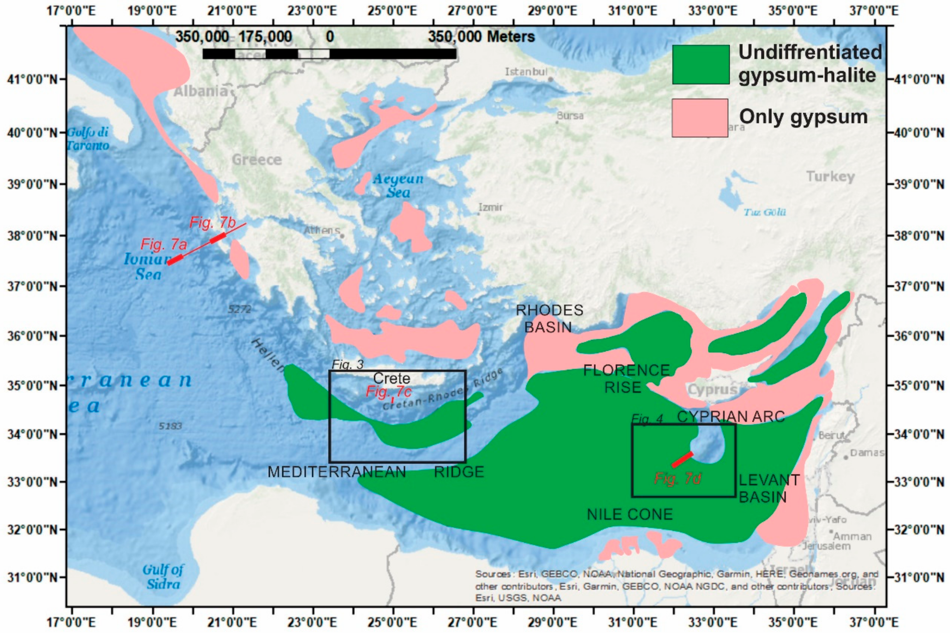
the detection of morphostructures on the seafloor related to shallow evaporite movement known as halokinesis.

In order to address the previous aims, bathymetric skeletons (medial axes from bathymetric data) are initially computed based on recently developed multiple filtering and skeletonization algorithms [6,16,18]. Then, the linear and curvilinear elements of the bathymetric skeleton are categorized based on criteria such as the strength of detection, their length, direction, and spatial distribution. Finally, we compare the automatically calculated bathymetric skeleton with ground truth data. Both case studies (the Southern Cretan offshore and the Levantine Basin, Figure 1) present bathymetric skeletons that are indicative of active tectonics. In addition, the bathymetric pattern in the Levantine Basin, southwest of the Eratosthenes Seamount, mostly presents morphological characteristics related to shallow salt movements (Figure 1).

Evaporites are water-soluble, layered, crystalline sedimentary rocks formed from surface or near surface brines in areas where high solar evaporation rates prevailed in the geological past [22]. Evaporation of seawater initially produces calcium carbonate (CaCO₃) followed by calcium sulfate in the form of gypsum (CaSO₄·2H₂O) or anhydrite (CaSO₄). The following mineral to form is halite (NaCl), commonly known as rock salt. Halite presents a low density (2160 kg/m³) and is mechanically weak, particularly under heavy overburden loading and high temperatures derived from its progressive burial. Thus, salt can flow like a visco-elastic fluid, even in cases where geologically strain rates are rapid [23]. Differential loading induced by gravitational forces, variable thermal conditions, or salt boundary displacement is the primary force inducing salt movement and usually results in vertical and lateral spreading or gliding along an inclined substratum [23]. Buried evaporite often manages to reach shallow depths below the seafloor, giving rise to specific morphological structures and further lineaments, as shown later in this work. Generally, lineaments are the surface expression of geological features such as fractures; faults; folds; geological contacts; rivers; streams; and other physiographic structures showing different origin, size, age, and depth [24,25,26,27]. They are important in recognizing geological structures on Earth’s surface related to the control and distribution of natural and mineral resources, geohazards, geothermal energy, and earthquakes. Tectonic lineaments relate to tectonic processes such as faulting and folding and are used in the production of structural maps.

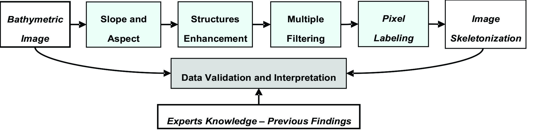
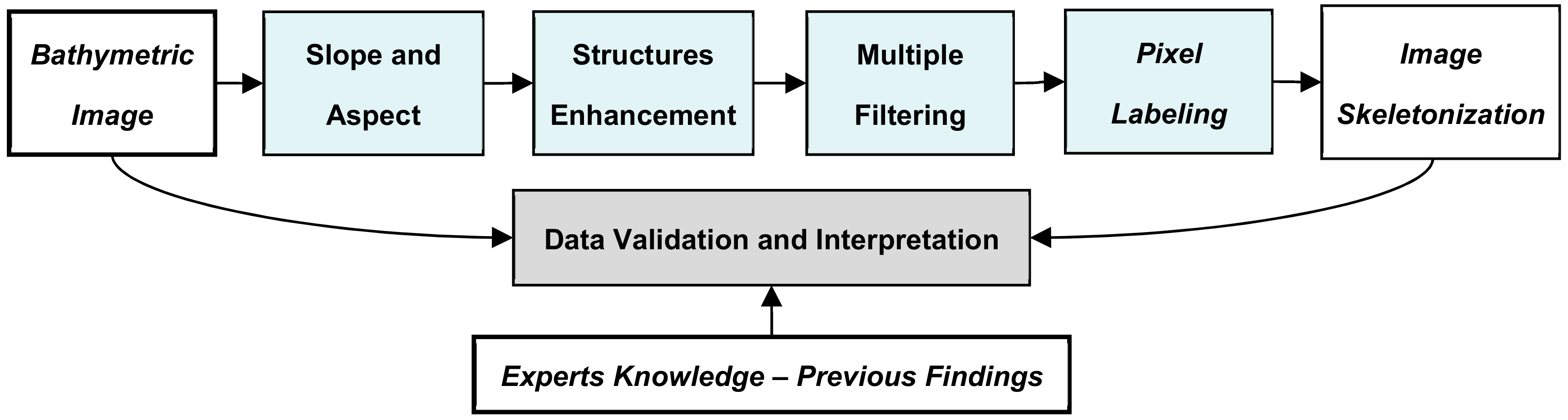
2. Materials and Methods

Medium- and high-resolution bathymetric data, from the open-file database EMODNet (European Marine Observatory and Data Network [28]) or compiled from various other sources [29,30,31,32], were primarily used in our research. Medium-resolution bathymetry derived from EMODNet comprises a grid/cell size of 0.25 arc minutes, while high-resolution bathymetry has a grid/cell size of 250 m.

The present methodology (Figure 2) continues the work of [16,17,18,33,34] that has been partially or in whole applied in previously published geological and environmental studies [6,35,36,37,38,39,40]. We summarize the steps of this methodology as follows:

2.1. Enhancement of the Seafloor Texture

Firstly, slope and aspect images as well their derivatives are computed. Then, the slope and aspect images are efficiently combined for the computation of the enhancement image F of seafloor texture (e.g., lineaments). The enhancement image F is computed as proposed in [16] and tested using onshore and offshore data [6,35,36,37,38,39,40].

F(p) = (S²(p) × SS(p) × SA(p))^1/4 is calculated based on the slope $S\left(p\right)$, the aspect $A\left(p\right)$, the first derivative of the slope SS (p), and the first derivative of the aspect SA(p) at point p (S(p)) of the topographic surface.

2.2. Multiple Filtering

In the enhancement image F, a step filter G(a,w) is applied, proposed in [34], to decrease noise and emphasize the linear and curvilinear structures of orientation a and width w.

$$I_g\left(a,w\right)=F\left(p\right)*G\left(a,w\right)$$

(1)

The filter $G\left(a,w\right)$ was constrained to be zero mean. In addition, the filter energy is normalized to one under any orientation and width (filter parameters), so that the responses of different angles and widths are comparable, respectively.

In order to enhance the curvilinear structures under any orientation and width, the image $I_m$ is computed by getting the maximum of the corresponding pixel values of $I_g\left(a,w\right)$.

2.3. Pixel Labeling

The preliminary goal of skeletonization is to classify I_m pixels into three classes, C₁, C₂, and C₃, with label numbers 1, 2, and 3, respectively:

C₁: The pixels corresponding to curvilinear structures.

C₂: The pixels uncertain to correspond to curvilinear structures. We decide for them in the last step, based on the other classes’ classification (C₁ and C₃).

C₃: The pixels that do not correspond to curvilinear structures.

The definition of the above classes is based on the hysterisis thresholding technique, which has been used on edge detection problem [41]. According to hysterisis thresholding, two thresholds, T_l (low) and T_h (high), are used to initially classify the pixels into three classes (C₁, C₂, and C₃). The advantage of this thresholding type is the exclusion of some connected point groups [42]. In the proposed scheme, the thresholds T_l and T_h are automatically estimated based on the median value of I_m values (Med).

• T_l is given by the mean value of I_m values that reveal a value lower than Med.
• T_h is given by the mean value of I_m values that reveal a value higher than Med.

Let B_i be the image of initial pixel classification into classes C₁, C₂, and C₃ and I_m(p) and mv(p) to denote the value of image I_m on pixel p and the median value of the nine pixel-neighborhood of pixel p in I_m, respectively.

• If I_m(p) ≥ T_h and I_m(p) > mv(p), p is classified to C₁, as its value is very high compared with the image (I_m(p) ≥ T_h) and with its neighbourhood (I_m(p) > mv(p)).
• Else, if I_m(p) ≥ T_h or (I_m(p) > T_l and I_m(p) > mv(p)), p is classified to C₂. This is true if the pixel value is high compared with the image, but it is not high enough compared with its neighbourhood, or reversely.
• Otherwise, p is classified to C₃.

Finally, a region growing-based method is applied on pixels of C₂ class to provide the final pixel labeling into classes C₁ and C₃. Let B_f be the image of final pixel classification into classes C₁ and C₃. According to the method, the pixels of C₂ class are classified to C₁ if they are connected to a pixel of C₁; otherwise, they are classified to C₃ class.

Image skeletonization (thin curvilinear structure detection) (B_t) is provided, if we change the second rule of classification to class C₂, removing the case of I_m(p) ≥ T_h.

3. Results

3.1. Automatically Calculated Bathymetric Skeleton

Image skeletonization aims to enhance shape analysis and data interpretation. Figure 3 and Figure 4 illustrate the results of the multiple filtering and skeletonization for both the Southern Cretan offshore and the area on, east, and southwest of the Eratosthenes Seamount, using the bathymetric data as input. The output of the multiple filtering approach for the Southern Cretan offshore and the area on, east, and southwest of the Eratosthenes Seamount is illustrated in Figure 3a and Figure 4a, respectively. The strong and weak detections are depicted with yellow and blue colors, respectively. Finally, Figure 3b and Figure 4b indicate the outcome of the thin curvilinear structure detection (skeletonization) using colour lines, projected on the original bathymetric relief. The red lines correspond to strongly detected linear and curvilinear elements, while the blue lines correspond to weak ones. The texture of the skeleton and changes in specific segments of the images are shown in Figure 3b and Figure 4b. The differences in the skeleton texture possibly relate to (a) sedimentation rates, (b) the degree of geodynamic activity in a certain area, (c) fluid and mass transfers, (d) slope instability processes, and (e) the activity of gravity (gliding) tectonics. Because of the differences in the skeleton texture, we divided both study areas in sub-regions (A, B, C and A’, B’, C’), respectively, based on the following criteria:

• The strength of the detection using the color scale shown in Figure 3a and Figure 4a ranging from 0 (blue) to 550 (yellow) with no units;
• The length of lineaments (short, medium, long);
• The direction of lineaments;
• The spatial distribution of the lineaments (sparse, medium, dense).

More specifically, the sub-regions A, B, C and A’, B’, C’ (Figure 3a,b and Figure 4a,b) show the following characteristics taking into account the above criteria:

• Sub-region A: Located in the Southern Cretan offshore (Ptolemy and Pliny Trenches including Gavdos high), characterized by medium to long in length and medium to sparse distributed lineaments generally trending NE–SW, NW–SE, and E–W, which present high detection strength (Figure 3a,b).
• Sub-region B: Located in the Southern Cretan offshore (Strabo Trench and the region west of Gavdos high) characterized by short to medium in length and medium to dense distributed lineaments trending to all directions (Figure 3a,b). The lineaments in the southeastern part of sub-region B present high detection strength, while those in the southwestern part of sub-region B present low detection strength (Figure 3a).
• Sub-region C: Located in the Southern Cretan offshore (Mediterranean Ridge) characterized by medium to long in length and medium to sparse distributed lineaments. Lineaments, close to the limit with sub-regions B and C, present similar orientation with this limit (Figure 3a,b). In addition, the lineaments near to the limit with sub-regions B and C present high detection strength (Figure 3a). The lineaments away from the limit with sub-regions B and C are generally short in length, medium to sparse distributed, and show no prevailing orientation (Figure 3a,b).
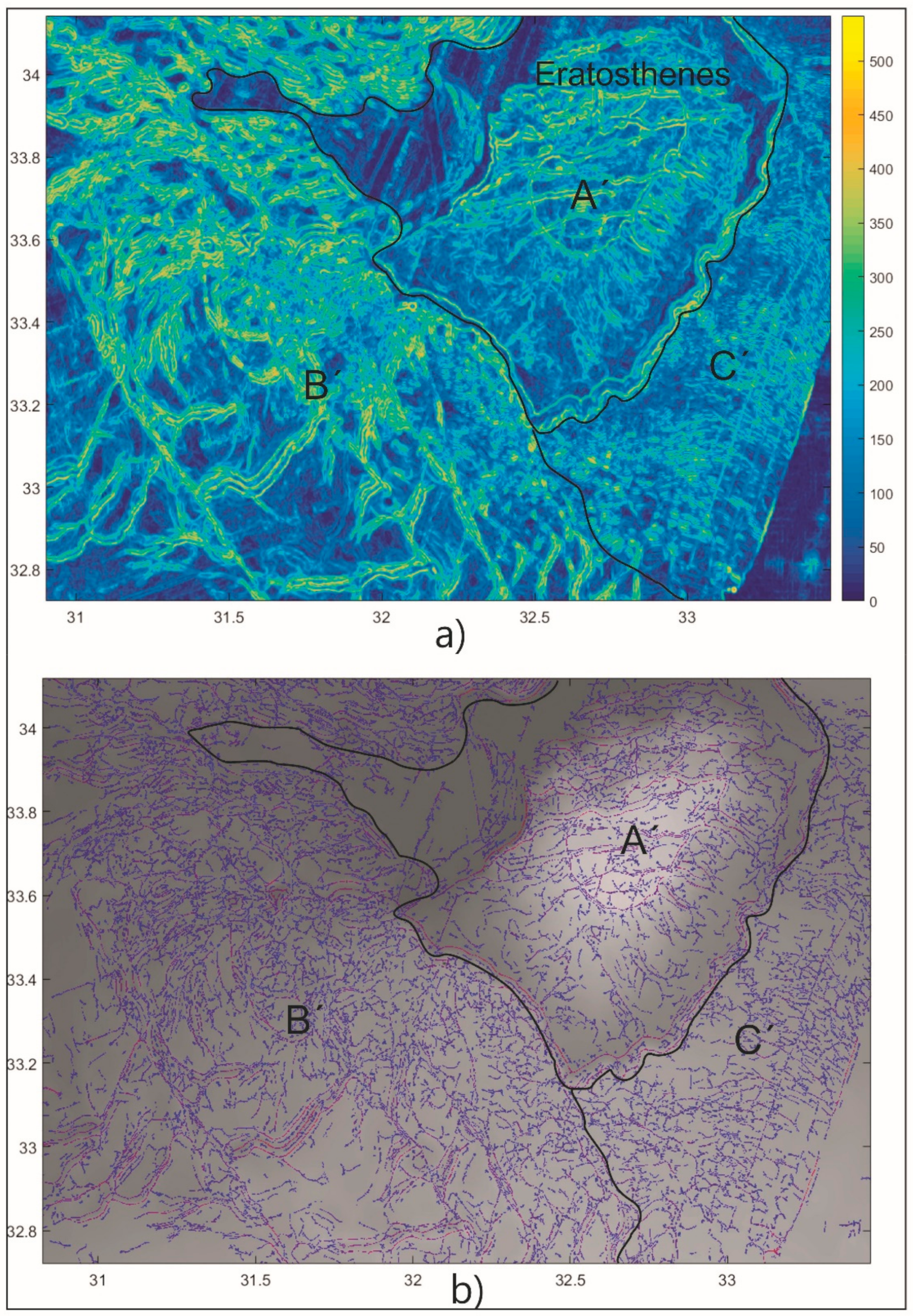
• Sub-region A’: Located on and west of the Eratosthenes Seamount characterized by (a) the presence of strong detected E–W trending, medium to long in length, and medium to sparse distributed lineaments on the Eratosthenes Seamount; and (b) very few, weak detected lineaments west of the Eratosthenes Seamount (Figure 4a,b).
• Sub-region B’: Located southwest of the Eratosthenes Seamount characterized by (a) strong detected, NE–SW trending lineaments intersected by a group of NW–SE trending lineaments, both long in length and sparse distributed; and (b) medium to weak detected lineaments with no prevailing orientation that are short in length and sparse to medium distributed (Figure 4a,b).
• Sub-region C’: Located east and southeast of the Eratosthenes Seamount characterized by generally weak detected, short in length and medium to sparse distributed lineaments that generally trend E–W to NW–SE (Figure 4a,b).

3.2. Comparison with Ground Truth Data

In Figure 5a,b, we present the comparison of the automatically calculated bathymetric skeleton with ground truth data for two selected areas. A significant part of the linear and curvilinear elements of the bathymetric skeleton is expected to correspond to tectonic lineaments, as both areas are strongly influenced by intense geodynamic activity related to different mechanisms.

The seafloor topography of the Southern Cretan Margin is strongly associated with transtensional movements in the upper 10–15 km of the crust, while transpression prevails below these depths [43]. Small-scale domes due to Messinian evaporitic intrusions may locally deform the recent stratigraphic successions (Pliocene–Quaternary) of the Southern Cretan Margin. Specifically, Figure 5a presents the automatically detected linear and curvilinear elements for the wide area of Gavdos Rise in South Crete. The red arrows show the most prominent automatically detected tectonic lineaments related to already reported geological faults [43,44,45]. Figure 6a,b present in more detail how we implemented the validation of the automatically detected tectonic lineaments. This figure resulted from the overlay of the geological faults (in red) [43,44,45] with the automatically detected skeleton. According to our previous work [16], the proposed method with linear patterns selection algorithm (LPSA) yields approximately 75% of the automatic detected lineaments to coincide either in location or in direction with the geological faults from ground truth data. The methodology in this work yields approximately 85% of the geological faults (thick red lines) to coincide in both location (less than 0.5 arc-minutes) and direction (less than 10 degrees) with the corresponding part of the bathymetric skeleton, meaning that the recall of the proposed method is about 85% (Figure 6b). Thus, there is a strong correlation between the automatically detected tectonic lineaments from the bathymetric skeleton (Figure 6) and those reported from previous studies [43,44,45]. In addition, a significant amount of information concerning the presence of additional tectonic lineaments is shown in Figure 5a, possibly related to primary or secondary fracture systems that should be investigated in the future.

The deformation of the area southwest of the Eratosthenes Seamount is mostly driven by salt tectonics related to the presence of underlying thick Messinian evaporites triggering processes of regional gravity spreading and gliding [46]. Specifically, the authors of [46], based on seismic and swath bathymetric data for this area, reported the presence of basins anchored within pre-Messinian sequences. This is because of massive salt removal and displacement of the salt/sediment system to areas with smoother slopes. Two examples of such areas, indicated by green line, are shown in Figure 5b. These areas (Figure 5b) are limited by distinctive, linear or curvilinear, continuous, strongly detected lineaments that probably correspond to large-scale geological faults [46,47]. In addition, these areas enclose curved morphological structures, whose distribution and morphology refer to salt flow. This argument is based on the correlation of the lineaments in these two areas (Figure 5b) with the seafloor morphology reported by [6,47,48]. In addition, the authors of [48] reported that, for the Central Red Sea, strongly influenced by salt flow, the morphology of the sedimentary cover on top of the moving salt often includes downslope ridges and troughs, along-slope ridges, areas of rough topography, as well as step like morphology at the flow fronts. The formation of brines in several deeps is the result of the dissolution of the Miocene evaporites upper part, and this can explain the irregular seafloor topography (vertical relief) close to the flow fronts [48]. While the origin of the downslope and along-slope ridges observed on the proposed salt flows cannot be definitely solved, their striking morphological similarity, where present, with features observed on ice glaciers or related to submarine mass movement indicates that sediment flow actually takes place near the Red Sea central trough [48]. In this work, we used the findings of [46,47,48] to interpret and further demonstrate how the automatically detected skeleton can assist the detection of shallow salt movements strongly related to potentially hydrocarbon-rich areas such as the wide area southwest of the Eratosthenes Seamount.

4. Discussion

4.1. Seafloor Deformation due to Halokinesis and Tectonism

The term “halokinesis” is used for autonomous salt movements due to heterogeneous density stratification in the crust [49,50]. The Mediterranean Basin is considered as the largest intracontinental deep-water basin bordered by Europe and Afro-Arabia, being one the world’s largest salt-bearing super giants (Figure 1). Two main salt geological intervals occur in the Mediterranean Basin; Triassic-Lower Jurassic salt and Upper Miocene (Messinian) salt (see Figures 8.5, 8.7, and 8.8 in [8]). Examples of seismic reflection (i.e., the most reliable ground truth method for imaging earth’s crust), showing overburden and related seafloor deformation due to halokinesis, are shown in Figure 7. Figure 7a,b present migrated seismic sections from line ION-7 crossing the Ionian Basin [51], corresponding to both intrusions of Messinian and Triassic evaporites. Figure 7a images the seafloor and underlying strata in the Ionian Abyssal Plain to reveal that Messinian salt deforms the overlying Pliocene-Quaternary strata. This kind of morphology is the so-called ‘cobblestone’ morphology [52,53]. The term ‘cobblestone’ morphology is used when recognizing small-scale, topographic bathymetric features with short wavelengths, a pattern primarily associated with small scale, diapiric movements. Figure 7b presents the seafloor deformation due to diapiric movements of Triassic evaporites in the hanging-wall anticlines of pre-existing thrusts [51,54,55]. Seafloor deformation due to the diapiric movements of Triassic evaporites is clearly characterized by larger scale topographic highs compared with the deformation due to the diapiric movements of the Messinian salts. Figure 7c shows an example from Southern Crete (Ptolemy Trough), where the seafloor is only slightly deformed as a result of halokinesis [43]. In Figure 7d, very moderate seafloor deformation in the form of small-scale ridges and troughs is visible in the NE–SW trending profile located SW of the Eratosthenes Seamount [56]. At this point, we point out that the deformation of the Pliocene-Pleistocene sequence overlying the Messinian salt in salt-rich basins around the Eratosthenes Seamount in the Eastern Mediterranean has been confirmed by abundant studies over many decades [46,47,48,56,57,58,59,60,61,62,63,64,65,66,67,68,69,70,71,72,73,74,75,76,77].

The bathymetric pattern related to salt presents distinct differences when compared with the bathymetric pattern related to intense tectonic activity. In [6], a comparison of the bathymetric patterns on and north of the Eratosthenes Seamount in Eastern Mediterranean proved that the present seafloor morphology north of Eratosthenes Seamount relates to shallow salt movements, creating a chaotic pattern. On the contrary, the bathymetric pattern on the Eratosthenes Seamount relates to the action of E–W trending geological faults. Going one step forward in this work, we apply multiple filtering and skeletonization to (a) correlate the automatically detected pattern of Gavdos Rise in Southern Crete with ground truth data (Figure 5a and Figure 6) and (b) detect patterns related to shallow salt movements southwest of the Eratosthenes Seamount (Figure 5b). Taking into account [6] and the present work, we report the following:

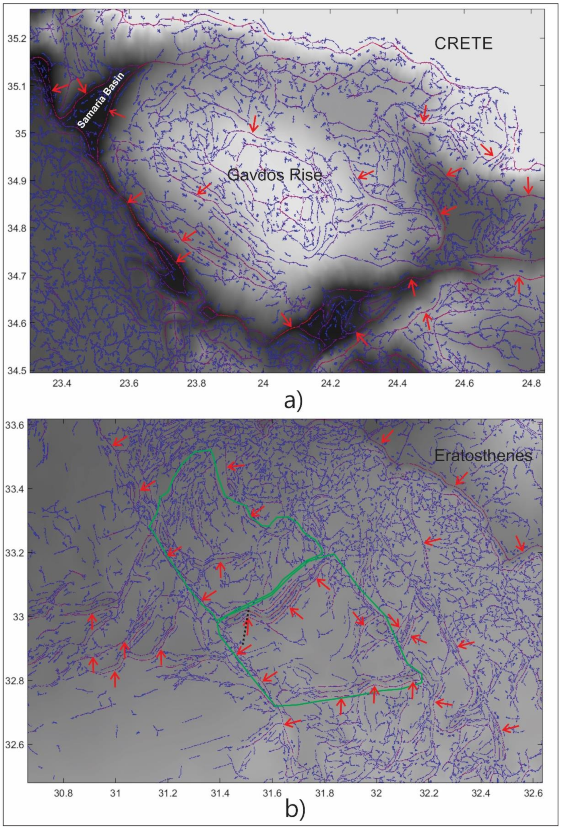
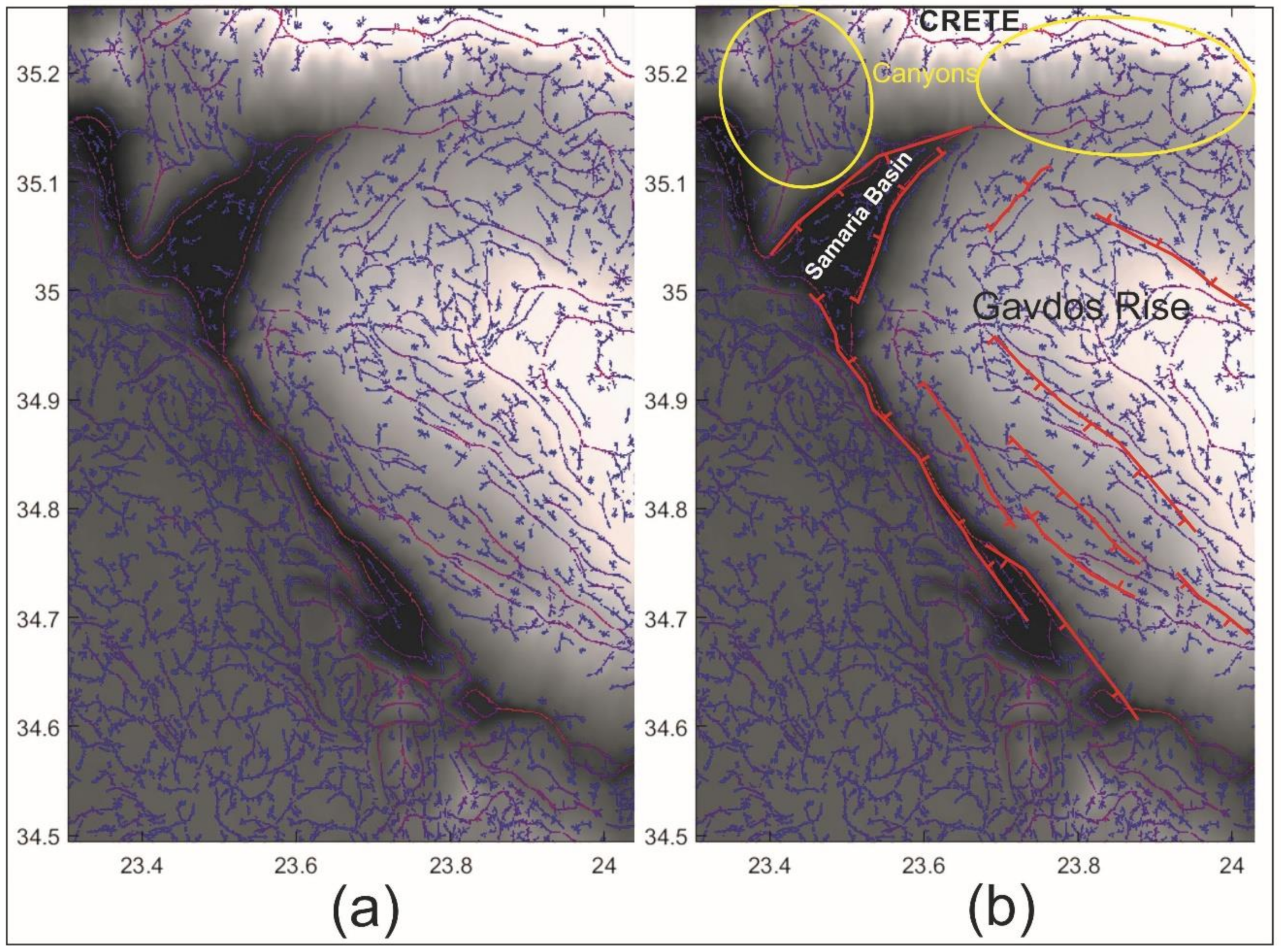
• Well-distinguished groups of lineaments trending to specific directions (Figure 5a and Figure 6) characterize the bathymetric pattern related to areas mostly affected by tectonism. The detection strength of the lineaments for these groups is generally high (red and yellow colors in Figure 3a and Figure 6);
• Morphostructures on the seafloor related to shallow salt movement (halokinesis) are recognized based on flow like characteristics such as (a) irregular seafloor topography, (b) downslope ridges and troughs, (c) presence of flow lobes (d) along-slope ridges and areas of rough topography, and (e) steplike morphology. In addition, areas with seafloor related to salt movements may be limited by distinctive, linear or curvilinear, continuous, long, and strongly detected lineaments that probably correspond to large-scale geological faults (Figure 5b, area indicated by green line).

Considerable work on the automatic extraction of geological lineaments has been published in the last years. The authors of [19] developed an algorithm that is based on tensor voting coupled Hough transform, aiming to extract geological lineaments from DEM and Landsat 8 OLI for the Loess areas in Baoji, China. Later, the authors of [78] proved that the extraction of lineaments is affected by the differences in the vertical accuracy. Specifically, the number of extracted lineaments as well as their length and density increase when the accuracy of the DEM increases. Recently, the authors of [79] managed to extract geological lineaments for a mine area in China based on wavelet edge detection and tracking by hillshade. However, all three previously mentioned works used land DEMs in the experimental phase supported by an abundance of ground truth data to validate their results. On the contrary, the present work used marine DEMs of considerably large areas in Eastern Mediterranean with limited ground truth data and not of very high resolution. However, multiple filtering and skeletonization seem to be effective for the automatic extraction of tectonic lineaments and salt-related morphostructures in bathymetric data even when bathymetric data are not of very high accuracy.

4.2. The Contribution of Multiple Filtering and Skeletonization in Marine Geology and Geophysics

Multiple filtering and skeletonization present a wide application on different problems of computer vision and pattern recognition with significant real-world applications in remote sensing [19,34,78,79,80,81], security [82], medicine [83], and computer graphics [84], especially for the identification and modelling of structures. Thus, these techniques, as previously shown, can significantly assist the interpretation of bathymetric and geophysical images to recognize seafloor and further subsurface structures. Specifically, multiple filtering and skeletonization can be applied in the following ways:

• prior to marine mapping at the stage where already available digitized data are reprocessed and evaluated, aiming to accurately specify the research targets and reduce the time and financial cost of the entire marine research;
• in digital bathymetric data acquired through remote sensing techniques or marine surveying.

The combination of multiple filtering and skeletonization techniques to identify tectonic lineaments and patterns related to evaporite movements with seafloor expression presents several advantages:

• Both are fast and simple methods with linear computational complexity concerning the image area, yielding high accuracy detections, as shown in Figure 3, Figure 4, Figure 5 and Figure 6 of Section 3.
• Multiple filtering is scale and orientation invariant [78].
• The skeleton accurately reflects the shape of the original image, preserving the topological properties (homotopy) and symmetry of the object. It holds that the stability of these methods is connected to the data quality (Figure 3, Figure 4 and Figure 5).
• Automatic identification does not require any ground truth data or training process as the popular deep learning (neural networks)-based methods [85], which cannot be applied in most of the cases, owing to unavailable or very limited ground truth data.
• The detection strength, the length, the direction of lineaments, as well as their spatial distribution are robust criteria for their sorting and further geological interpretation.

The only drawback of the proposed scheme is some possible false detections after the skeletonization process, as skeletonization is sensitive to minor boundary deformations and image noise. Some of them can be automatically removed via skeleton pruning [86], if they concern skeleton parts of well-detected medial axes. In addition, segments with unpredictable and irregular orientation can be automatically detected as outliers, if we compare their orientation with the orientation of the other detected medial axes in a neighborhood. This part can be also included in our future work.

5. Conclusions

This work demonstrates a fast and effective methodology of bathymetric analysis based on image multiple filtering and skeletonization. The experimental results with bathymetric data from the Southern Cretan offshore and the Levantine Basin (on, east, and southwest of the Eratosthenes Seamount) and comparison with ground truth data indicate the reliable, time-effective, and cost-effective performance of the proposed scheme. As a conclusion:

• The skeleton, provided by the application of the present scheme, preserves the shape and symmetry of the original lineaments. In addition, the tracing of the lineaments is accurate, taking into account their location, direction, and spatial extend. Obviously, the accuracy of lineaments automatic extraction depends on DEM’s accuracy.
• Multiple filtering and skeletonization are independent in training process, so it works even in cases of limited ground truth data.
• Robust criteria, such as the strength of the detection, the length, the direction, the spatial distribution, and/or density of the lineaments, are valuable for the interpretation of the bathymetric patterns. Consequently, either seafloor morphology related with intense tectonic activity or evaporite movements with seafloor expression can be recognized and further interpreted to assist the structural analysis of potentially hydrocarbon-rich areas.

Ongoing work targets (a) the automatic erasing of false detections and the combination of this method with deep learning when more ground data are available, and (b) the prediction of possible natural gas or oil deposits in combination with related datasets.

References

1. Micallef, A.; Krastel, S.; Savini, A. (Eds.) Introduction. In Submarine Geomorphology; Springer: Berlin, Germany, 2018; pp. 1–9. [Google Scholar]
2. Lecours, V.; Dolan, M.F.J.; Micallef, A.; Lucieer, V.L. A review of marine geomorphometry, the quantitative study of the seafloor. Hydrol. Earth Syst. Sci. 2016, 20, 3207–3244. [Google Scholar] [CrossRef] [Green Version]
3. Lucieer, V.L.; Lecours, V.; Dolan, M.F.J. Marine Geomorphometry; MDPI: Basel, Switzerland, 2019; pp. 1–402. [Google Scholar]
4. Parsons, B.; Sclater, J.G. An analysis of the variation of ocean floor bathymetry and heat flow with age. J. Geophys. Res. 1977, 82, 803–827. [Google Scholar] [CrossRef]
5. Wessel, P.; Chandler, M.T. The spatial and temporal distribution of marine geophysical surveys. Acta Geophys. 2011, 59, 55–71. [Google Scholar] [CrossRef]
6. Kokinou, E.; Panagiotakis, C. Structural pattern recognition applied on bathymetric data from the Eratosthenes Seamount (Eastern Mediterranean, Levantine Basin). Geo-Mar. Lett. 2018, 38, 527–540. [Google Scholar] [CrossRef]
7. Camerlenghi, A. Drivers of Seafloor Geomorphic Change. In Submarine Geomorphology; Micallef, A., Krastel, S., Savini, A., Eds.; Springer: Cham, Switzerland, 2018; pp. 135–159. [Google Scholar]
8. Belenitskaya, G. Salt Systems of the Earth: Distribution, Tectonic and Kinematic History, Salt-Naphthids Interrelations, Discharge Foci, Recycling; Wiley Online Library: Hoboken, NJ, USA, 2018; pp. 1–693. [Google Scholar]
9. Kweon, I.S.; Kanade, T. Extracting topographic terrain features from elevation maps. CVGIP Image Underst. 1994, 59, 171–182. [Google Scholar] [CrossRef]
10. Miliaresis, G.C.; Argialas, D. Segmentation of physiographic features from the global digital elevation model/gtopo30. Comput. Geosci. 1999, 25, 715–728. [Google Scholar] [CrossRef]
11. Dinesh, S. Extraction of mountains from digital elevation models using mathematical morphology. GIS Dev. Malays. 2006, 1, 16–19. [Google Scholar]
12. Iwahashi, J.; Pike, R.J. Automated classifications of topography from dems by an unsupervised nested-means algorithm and a three-part geometric signature. Geomorphology 2007, 86, 409–440. [Google Scholar] [CrossRef]
13. Booth, A.M.; Roering, J.J.; Perron, J.T. Automated landslide mapping using spectral analysis and high-resolution topographic data: Puget sound Lowlands, Washington, and Portland hills, Oregon. Geomorphology 2009, 109, 132–147. [Google Scholar] [CrossRef]
14. Obu, J.; Podobnikar, T. Algorithm for karst depression recognition using digital terrain models. Geod. Vestn. 2013, 57, 260–270. [Google Scholar] [CrossRef]
15. Euillades, L.D.; Grosse, P.; Euillades, P.A. Netvolc: An algorithm for automatic delimitation of volcano edifice boundaries using dems. Comput. Geosci. 2013, 56, 151–160. [Google Scholar] [CrossRef]
16. Panagiotakis, C.; Kokinou, E. Linear Pattern Detection of Geological Faults via a Topology and Shape Optimization Method. IEEE J. Sel. Top. Appl. Earth Obs. Remote Sens. 2015, 8, 3–11. [Google Scholar] [CrossRef]
17. Micheal, A.A.; Vani, K. Automatic mountain detection in lunar images using texture of dtm data. Comput. Geosci. 2015, 82, 130–138. [Google Scholar] [CrossRef]
18. Panagiotakis, C.; Kokinou, E. Unsupervised Detection of Topographic Highs with Arbitrary Basal Shapes Based on Volume Evolution of Isocontours. Comput. Geosci. 2017, 102, 22–33. [Google Scholar] [CrossRef]
19. Han, L.; Liu, Z.; Ning, Y.; Zhao, Z. Extraction and analysis of geological lineaments combining a DEM and remote sensing images from the northern Baoji loess area. Adv. Space Res. 2018, 62, 2480–2493. [Google Scholar] [CrossRef]
20. Florinsky, I.V. Quantitative topographic method of fault morphology recognition. Geomorphology 1996, 16, 103–119. [Google Scholar] [CrossRef]
21. Florinsky, I.V. Digital Terrain Analysis in Soil Science and Geology, 2nd ed.; Elsevier: Amsterdam, The Netherlands, 2016; pp. 1–486. [Google Scholar]
22. Warren, J.K. Evaporites, a Geological Compendium, 2nd ed.; Springer: Berlin, Germany, 2016; pp. 1–1813. [Google Scholar]
23. Hudec, M.R.; Jackson, M.P.A. Terra infirma: Understanding salt tectonics. Earth-Sci. Rev. 2007, 82, 1–28. [Google Scholar] [CrossRef]
24. Hobbs, W.H. Lineaments of Atlantic Border region. Bull. Geol. Soc. Am. 1904, 15, 483–506. [Google Scholar] [CrossRef]
25. O’Leary, D.W.; Friedman, J.D.; Pohn, H.A. Lineament, linear, lineation: Some proposed new standards for old terms. Bull. Geol. Soc. Am. 1976, 87, 1463–1469. [Google Scholar] [CrossRef]
26. Makarov, V.I. Lineaments: Problems and trends of studies by remote sensing techniques. Izv. Vuz. Geol. Razv. 1981, 4, 109–115. (In Russian) [Google Scholar]
27. Florinsky, I.V. Global Lineaments: Application of Digital Terrain Modelling. In Advances in Digital Terrain Analysis. Lecture Notes in Geoinformation and Cartography; Zhou, Q., Lees, B., Tang, G., Eds.; Springer: Berlin/Heidelberg, Germany, 2008; pp. 365–382. [Google Scholar]
28. Berthou, P. EMODNET-the European marine observation and data network. Eur. Sci. Found. Mar. Board 2008, 10. [Google Scholar]
29. Benkhelil, J.; Mart, Y.; Mascle, J.; Woodside, J.M.; The Prismed II Scientific Party. Recent morphostructural evolution of the Eratosthenes Seamount: Initial Results of the Prismed II Cruise. European Union of Geosciences/EUG 10, Strasbourg (France). J. Conf. Abs. 1999, 4, 756, Terra Abstracts 11. [Google Scholar]
30. CIESM/Ifremer Medimap Group; Loubrieu, B.; Mascle., J. Morpho-bathymetry of the Mediterranean Sea. CIESM: Monte Carlo, Monaco, 2008. [Google Scholar]
31. Huebscher, C. RV MARIA S. MERIAN, Cruise Report MSM14/L3 Eratosthenes Seamount/Eastern Mediterranean Sea 2010; DFG Senatskommission für Ozeanographie: Bremen, Germany, 2012. [Google Scholar]
32. U.S. Department of Commerce, National Oceanic and Atmospheric Administration, National Geophysical Data Center. 2-Minute Gridded Global Relief Data (ETOPO2v2). 2006. Available online: http://www.ngdc.noaa.gov/mgg/fliers/06mgg01.html (accessed on 12 May 2020).
33. Kokinou, E.; Panagiotakis, C.; Sarris, A. Application of Skeletonization on Geophysical Images. In Proceedings of the XIX Congress of the Carpathian Balkan Geological Association, Thessaloniki, Grecce, 23–26 September 2010; Volume 99, pp. 338–343. [Google Scholar]
34. Panagiotakis, C.; Kokinou, E.; Sarris, A. Curvilinear Structure Enhancement and Detection in Geophysical Images. IEEE Trans. Geosci. Remote Sens. 2011, 49, 2040–2048. [Google Scholar] [CrossRef]
35. Alves, T.M.; Kokinou, E.; Zodiatis, G.; Lardner, R.; Panagiotakis, C.; Radhakrishnan, H. Modelling of oil spills in confined maritime basins: The case for early response in the Eastern Mediterranean Sea. Environ. Pollut. 2015, 206, 390–399. [Google Scholar] [CrossRef] [PubMed] [Green Version]
36. Alves, T.; Kokinou, E.; Zodiatis, G.; Lardner, R. Hindcast, GIS and susceptibility modelling to assist oil spill clean-up and mitigation on the southern coast of Cyprus (Eastern Mediterranean). Deep-Sea Res. Part II 2016, 133, 159–175. [Google Scholar] [CrossRef]
37. Alves, T.M.; Kokinou, E.; Zodiatis, G.; Radhakrishnan, H.; Panagiotakis, C.; Lardner, R. Multidisciplinary oil spill modeling to protect coastal communities and the environment of the Eastern Mediterranean Sea. Sci. Rep. 2016, 6, 36882. [Google Scholar] [CrossRef]
38. Kokinou, E. Geomorphologic features of the marine environment in Eastern Mediterranean using a modern processing approach. In Proceedings of the IAMG 2015, the 17th Annual Conference of the International Association for Mathematical Geosciences, Freiberg, Germany, 5–13 September 2015; Schaeben, H., Tolosana Delgado, R., van den Boogaart, G.K., van den Boogaart, R., Eds.; IAMG: Freiberg, Germany, 2015; pp. 436–445. [Google Scholar]
39. Andronikidis, N.; Kokinou, E.; Vafidis, A.; Kamberis, E.; Manoutsoglou, E. Deformation patterns in the southwestern part of the Mediterranean Ridge (South Matapan Trench, Western Greece). Mar. Geophys. Res. 2018, 39, 475–490. [Google Scholar] [CrossRef]
40. Toulia, E.; Kokinou, E.; Panagiotakis, C. The contribution of pattern recognition techniques in geomorphology and geology: The case study of Tinos Island (Cyclades, Aegean, Greece). Eur. J. Remote Sens. 2018, 51, 88–99. [Google Scholar] [CrossRef]
41. Canny, J. A computational approach to edge detection. IEEE Trans. Pattern Anal. Mach. Intell. 1986, 8, 679–698. [Google Scholar] [CrossRef]
42. Kermad, C.D.; Chehdi, K. Automatic image segmentation system through iterative edge-region co-operation. Image Vis. Comput. 2002, 8, 541–555. [Google Scholar] [CrossRef] [Green Version]
43. Kokinou, E.; Alves, T.M.; Kamberis, E. Structural decoupling on a convergent forearc setting (Southern Crete, Eastern Mediterranean). Geol. Soc. Am. Bull. 2012, 124, 1352–1364. [Google Scholar] [CrossRef]
44. IGME (Institute of Mineral and Geological Exploration). Seismotectonic Map of Greece. Scale 1:500000; IGME: Athens, Greece, 1989. [Google Scholar]
45. Manta, K.; Rousakis, G.; Anastasakis, G.; Lykousis, V.; Sakellariou, D.; Panagiotopoulos, I.P. Sediment transport mechanisms from the slopes and canyons to the deep basins south of Crete Island (southeast Mediterranean). Geo-Mar. Lett. 2019, 39, 295–312. [Google Scholar] [CrossRef]
46. Mascle, J.; Sardou, O.; Loncke, L.; Migeon, S.; Camera, L.; Gaullier, V. Morphostructure of the Egyptian continental margin: Insights from swath bathymetry surveys. Mar. Geophys. Res. 2006, 27, 49–59. [Google Scholar] [CrossRef]
47. Schattner, U. What triggered the early-to-mid Pleistocene tectonic transition across the entire eastern Mediterranean? Earth Planet. Sci. Lett. 2010, 289, 539–548. [Google Scholar] [CrossRef]
48. Feldens, P.; Mitchell, N. Salt flows in the Central Red Sea. In The Red Sea: The Formation, Morphology, Oceanography and Environment of a Young Ocean Basin; Rasul, N., Stewart, I., Eds.; Springer: Berlin/Heidelberg, Germany, 2015; pp. 205–218. [Google Scholar]
49. Trusheim, F. Über Halokinese und ihre Bedeutung für die strukturelle Entwicklung Norddcutschlands. Z. Deutch. Geol. Ges. 1957, 198, 111–151. [Google Scholar]
50. Trusheim, F. Mechanism of salt migration in northern Germany. AAPG Bull. 1960, 44, 1519–1540. [Google Scholar]
51. Kokinou, E.; Kamberis, E.; Vafidis, A.; Monopolis, D.; Ananiadis, G.; Zelilidis, A. Deep seismic reflection data from offshore Western Greece: A new crustal model for the Ionian Sea. J. Pet. Geol. 2005, 28, 81–98. [Google Scholar] [CrossRef]
52. Hersey, J.B. Sedimentary basins of the Mediterranean Sea. In Submarine Geology and Geophysics, Proceedings of the 17th Symposium of the Colston Research Society, London, UK, 5–9 April 1965; Whitard, W.F., Bradshaw, W., Eds.; Butterworths: London, UK, 1965; pp. 75–91. [Google Scholar]
53. Hsu, K.J.; Cita, M.B. The origin of the Mediterranean Evaporite. In Initial Reports of the Deep Sea Drilling Project; U.S. Government Printing Office: Washington, DC, USA, 1973; Volume 13, pp. 1203–1231. [Google Scholar]
54. Monopolis, D.; Bruneton, A. Ionian Sea (Western Greece): Its structural outline deduced from drilling and geophysical data. Tectonophysics 1982, 83, 227–242. [Google Scholar] [CrossRef]
55. Brooks, M.; Ferentinos, G. Tectonics and Sedimentation in the Gulf of Corinth and Zakynthos and Kefallinia channels, western Greece. Tectonophysics 1984, 101, 25–54. [Google Scholar] [CrossRef]
56. Kopf, A.; Vidal, N.; Klaeschen, D.; von Huene, R.; Krasheninnikov, V.A. Multi-channel seismic profiles across Eratosthenes Seamount and the Florence Rise reflecting the incipient collision between Africa and Eurasia near the island of Cyprus, Eastern Mediterranean. In Geological Framework of the Levant, Volume II: The Levantine Basin and Israel; Hall, J.K., Krasheninnikov, V.A., Hirsch, F., Benjamini, C., Flexer, A., Eds.; Historical Productions-Hall: Jerusalem, Israel, 2005; pp. 57–72. [Google Scholar]
57. Neev, D.; Almagor, G.; Arad, V.; Ginzburg, A.; Hall, J.K. The geology of the southeastern Mediterranean Sea. Geol. Surv. Isr. Bull. 1976, 68, 1051. [Google Scholar]
58. Ben-Avraham, Z. The structure and tectonic setting of the Levant continental margin, Eastern Mediterranean. Tectonophysics 1978, 46, 313–331. [Google Scholar] [CrossRef]
59. Garfunkel, Z.; Arad, V.; Almagor, G. The Palmahim disturbance and its regional setting. Geol. Surv. Isr. Bull. 1979, 72, 56. [Google Scholar]
60. Mart, Y.; Ben-Gai, Y. Some depositional patterns at continental margin of southeaster Mediterranean Sea. AAPG Bull. 1982, 66, 460–470. [Google Scholar]
61. Almagor, G.; Hall, J.K. Morphology of the continental margin off north-central Israel. Isr. J. Earth Sci. 1983, 32, 75–82. [Google Scholar]
62. Garfunkel, Z. Large-scale submarine rotational slumps and growth faults in the eastern Mediterranean. Mar. Geol. 1984, 55, 304–324. [Google Scholar] [CrossRef]
63. Frey-Martinez, J.; Cartwright, J.A.; Hall, B. 3D seismic interpretation of slump complexes: Examples from the continental margin of Israel. Basin Res. 2005, 17, 83–108. [Google Scholar] [CrossRef]
64. Gradmann, S.; Huebscher, C.; Ben-Avraham, Z.; Gajewski, D.; Netzband, G. Salt tectonics off northern Israel. Mar. Pet. Geol. 2005, 22, 597–611. [Google Scholar] [CrossRef]
65. Bertoni, C.; Cartwright, J.A. Controls on the basinwide architecture of late Miocene (Messinian) evaporites on the Levant margin (Eastern Mediterranean). Sediment. Geol. 2006, 188, 93–114. [Google Scholar] [CrossRef]
66. Bertoni, C.; Cartwright, J.A. Major erosion at the end of the Messinian Salinity Crisis: Evidence from the Levant Basin, Eastern Mediterranean. Basin Res. 2007, 19, 1–18. [Google Scholar] [CrossRef]
67. Loncke, L.; Gaullier, V.; Mascle, J.; Vendeville, B.; Camera, L. The Nile deep-sea fan: An example of interacting sedimentation, salt tectonics, and inherited subsalt paleotopographic features. Mar. Pet. Geol. 2006, 23, 297–315. [Google Scholar] [CrossRef]
68. Netzeband, G.; Huebscher, C.; Gajewski, D. The structural evolution of the Messinian evaporites in the Levantine Basin. Mar. Geol. 2006, 230, 249–273. [Google Scholar] [CrossRef]
69. Mart, Y.; Ryan, W. The Levant slumps and the Phoenician structures: Collapse features along the continental margin of the southeastern Mediterranean Sea. Mar. Geophys. Res. 2007, 28, 297–307. [Google Scholar] [CrossRef]
70. Cartwright, J.A.; Jackson, M.P.A. Initiation of gravitational collapse of an evaporate basin margin: The Messinian saline giant, Levant Basin, eastern Mediterranean. Geol. Soc. Am. Bull. 2008, 120, 399–413. [Google Scholar] [CrossRef]
71. Clark, I.R.; Cartwright, J.A. Interactions between submarine channel systems and deformation in deepwater fold belts: Examples from the Levant Basin, Eastern Mediterranean Sea. Mar. Pet. Geol. 2009, 26, 1465–1482. [Google Scholar] [CrossRef]
72. Gvirtzman, Z.; Reshef, M.; Buch-Leviatan, O.; Ben-Avraham, Z. Intense salt deformation in the Levant Basin in themiddle of the Messinian Salinity Crisis. Earth Planet. Sci. Lett. 2013, 379, 108–119. [Google Scholar] [CrossRef]
73. Reiche, S.; Huebscher, C. The Hecataeus Rise, easternmost Mediterranean: A structural record of Miocene-Quaternary convergence and incipient continent-continent-collision at the African-Anatolian plate boundary. Mar. Pet. Geol. 2015, 67, 368–388. [Google Scholar] [CrossRef]
74. Symeou, V.; Homberg, C.; Nader, F.H.; Darnault, R.; Lecomte, J.C.; Papadimitriou, N. Longitudinal and Temporal Evolution of the Tectonic Style Along the Cyprus Arc System, Assessed Through 2-D Reflection Seismic Interpretation. Tectonics 2018, 37, 30–47. [Google Scholar] [CrossRef] [Green Version]
75. Rouchy, J.M.; Caruso, A. The Messinian salinity crisis in the Mediterranean basin: A reassessment of the data and an integrated scenario. Sediment. Geol. 2006, 188, 35–67. [Google Scholar] [CrossRef]
76. Manzi, V.; Gennari, R.; Lugli, S.; Roveri, M.; Scafetta, N.; Schreiber, B.C. High frequency cyclicity in the Mediterranean Messinian evaporites: Evidence for solar–lunar climate forcing. J. Sediment. Res. 2012, 82, 991–1005. [Google Scholar] [CrossRef]
77. Roveri, M.; Flecker, R.; Krijgsman, W.; Lofi, J.; Lugli, S.; Manzi, V.; Sierro, F.J.; Bertini, A.; Camerlenghi, A.; De Lange, G.; et al. The Messinian Salinity Crisis: Past and future of a great challenge for marine sciences. Mar. Geol. 2014, 352, 25–58. [Google Scholar] [CrossRef]
78. Soliman, A.; Han, L. Effects of vertical accuracy of digital elevation model (DEM) data on automatic lineaments extraction from shaded DEM. Adv. Space Res. 2019, 64, 603–622. [Google Scholar] [CrossRef]
79. Xu, J.; Wen, X.; Zhang, H.; Luo, D.; Li, J.; Xu, L.; Yu, M. Automatic extraction of lineaments based on wavelet edge detection and aided tracking by hillshade. Adv. Space Res. 2020, 65, 506–517. [Google Scholar] [CrossRef]
80. Gournia, C.; Fakiris, E.; Geraga, M.; Williams, D.P.; Papatheodorou, G. Automatic Detection of Trawl-Marks in Sidescan Sonar Images through Spatial Domain Filtering, Employing Haar-Like Features and Morphological Operations. Geosciences 2019, 9, 214. [Google Scholar] [CrossRef] [Green Version]
81. Parker, J.R. Algorithms for Image Processing and Computer Vision, 2nd ed.; Wiley Publishing: Indianapolis, IN, USA, 2010; ISBN 0470643854. [Google Scholar]
82. Bounneche, M.D.; Boubchir, L.; Bouridane, A.; Nekhoul, B.; Ali-Chérif, A. Multi-spectral palmprint recognition based on oriented multiscale log-Gabor filters. Neurocomputing 2016, 205, 274–286. [Google Scholar] [CrossRef] [Green Version]
83. Panagiotakis, C.; Argyros, A. Region-based Fitting of Overlapping Ellipses and its Application to Cells Segmentation. Image Vis. Comput. 2020, 93, 103810. [Google Scholar] [CrossRef]
84. Panagiotakis, C.; Tziritas, G. Snake terrestrial locomotion synthesis in 3D virtual environments. Vis. Comput. 2006, 22, 86–98. [Google Scholar] [CrossRef]
85. Zhu, X.X.; Tuia, D.; Mou, L.; Xia, G.S.; Zhang, L.; Xu, F.; Fraundorfer, F. Deep learning in remote sensing: A comprehensive review and list of resources. IEEE Geosci. Remote Sens. Mag. 2017, 5, 8–36. [Google Scholar] [CrossRef] [Green Version]
86. Liu, H.; Wu, Z.H.; Zhang, X.; Hsu, D.F. A skeleton pruning algorithm based on information fusion. Pattern Recognit. Lett. 2013, 34, 1138–1145. [Google Scholar] [CrossRef]
Figure 1. Map of the wide area of Eastern Mediterranean Sea and corresponding distribution of Late Miocene (Messinian) salt. The data concerning the base map are from the ArcGIS 10 online database. Black rectangles correspond to the automatic detection of bathymetric structures.The red lines in this figure show the locations of the seismic reflection profiles shown later in this work where the seafloor is deformed owing to the presence of underlying salt. Recently, updated maps concerning the distribution of both Triassic and Messinian salts in the Mediterranean Sea have been presented in previous works [8].
Remotesensing 12 01538 g001
Figure 2. Flow-chart illustrating the methodology of the present work.
Remotesensing 12 01538 g002
Figure 3. Automatic detection of the seafloor skeleton in the Southern Cretan offshore using medium resolution (0.25 arc minutes) data from EMODNet (European Marine Observatory and Data Network) [28]. The reference system is WGS84. (a) The output of the multiple filtering approach [34]. Color scale corresponds to the strength of the detection ranging from 0 (blue) to 550 (yellow) with no units. (b) The skeleton (medial axes) overlain the bathymetric relief. The red lines correspond to strongly detected linear and curvilinear elements, while the blue lines correspond to weak ones. On the basis of signal texture (strength of the detection, length, direction, and spatial distribution of the lineaments), we divided the area into three sub-regions (A, B, and C).
Remotesensing 12 01538 g003
Figure 4. Automatic detection of the seafloor skeleton in the Levantine Basin (east and southwest of the Eratosthenes Seamount) using medium resolution (0.25 arc minutes) data from EMODNet (European Marine Observatory and Data Network) [28] and other sources [29,30,31,32]. The reference system is WGS84. (a) The output of the multiple filtering approach [34]. Color scale corresponds to the strength of the detection ranging from 0 (blue) to 550 (yellow) with no units. (b) The skeleton (medial axes) overlain the bathymetric relief. The red lines correspond to strongly detected linear and curvilinear elements, while the blue lines correspond to weak ones. On the basis of signal texture (strength of the detection, length, direction, and spatial distribution of the lineaments), we divided the area into three sub-regions (A’, B’, and C’).
Remotesensing 12 01538 g004
Figure 5. Comparison of the automatically detected linear and curvilinear elements with ground truth data. The red lines correspond to strongly detected linear and curvilinear elements, while the blue lines correspond to weak ones. Red arrows show the linear and curvilinear elements corresponding to strong automatic detection and they are in full agreement with previously reported geological faults in (a) the wide area of Gavdos Rise in South Crete [43,44,45] and (b) southwest of the Eratosthenes Seamount. Areas indicated by the closed green line are possibly affected by shallow salt movements [46,47,48].
Remotesensing 12 01538 g005
Figure 6. An example showing the comparison of the (a) automatically detected linear and curvilinear elements from the western part of Gavdos Rise in South Crete with (b) geological faults (thick red lines) from previous research [43,44,45] and references therein. The yellow ellipsis indicates areas of canyons [45].
Remotesensing 12 01538 g006
Figure 7. Seismic reflection profiles highlighting the styles of seafloor deformation due to the presence of underlying salt—see red rectangles. TWT corresponds to two way travel time. The locations of the seismic reflection sections are shown in Figure 1. These high-resolution 2D profiles image Messinian salt (a) in the Ionian Abyssal Plain, together with underlying Triassic evaporites; (b) around the Kefallinia Diapir [51]; (c) N–S trending high-resolution 2D profile from the Ptolemy trough, Southern Crete (Greece), imaging very moderate deformation of the seafloor owing to halokinesis [43]; (d) NE–SW trending high-resolution 2D profile located SW of the Eratosthenes Seamount revealing the presence of Messinian salt in the Levantine Basin [56].
Remotesensing 12 01538 g007