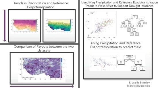
Identifying Precipitation and Reference Evapotranspiration Trends in West Africa to Support Drought Insurance

 , , , , and
Abstract
1. Introduction
1.1. Farming under Uncertainty
1.2. Agroclimatic Indicators in West Africa
1.3. Index Insurance in West Africa
1.4. Objectives
2. Materials and Methods
2.1. Data
2.2. Trend Analysis
2.3. Index Design
2.4. Heidke Skill Score
2.5. Linear Regression
2.6. Classification and Regression Tree Analysis
3. Results
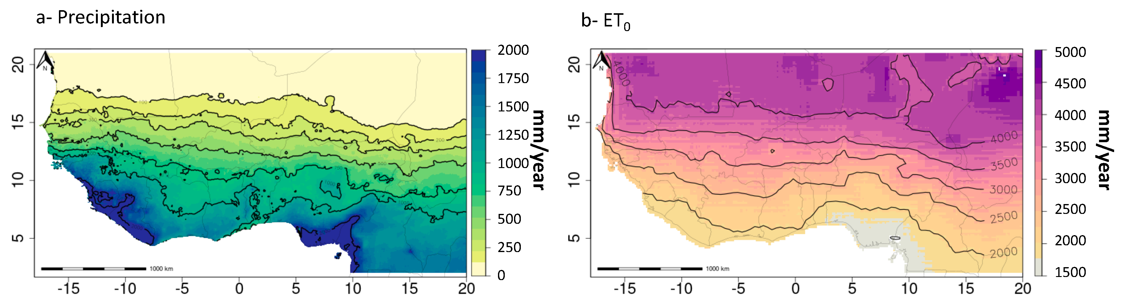
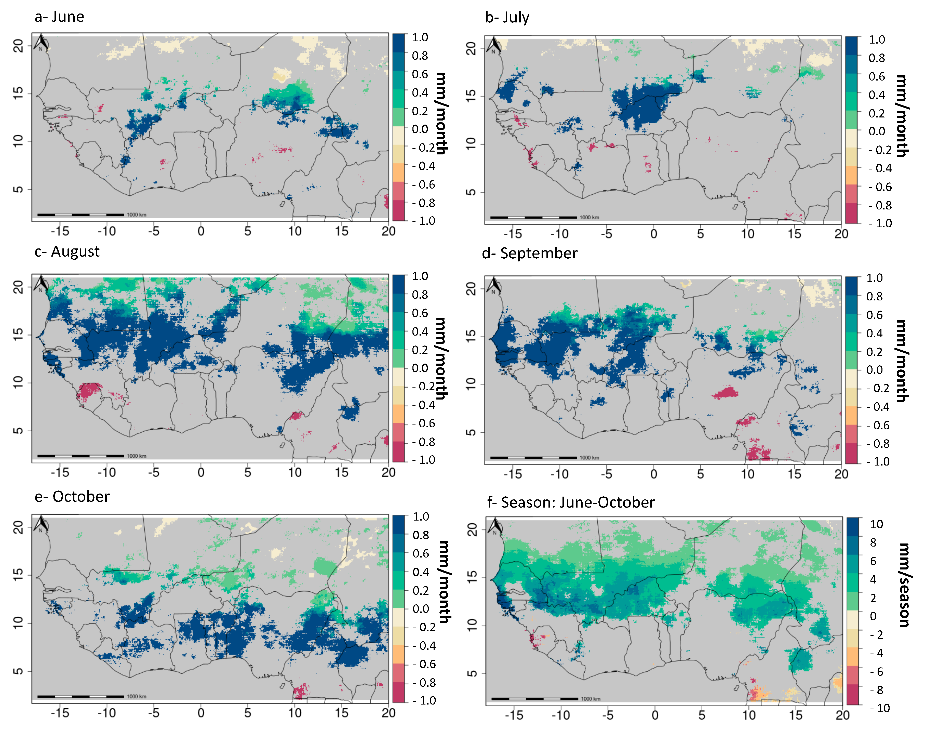
3.1. Precipitation
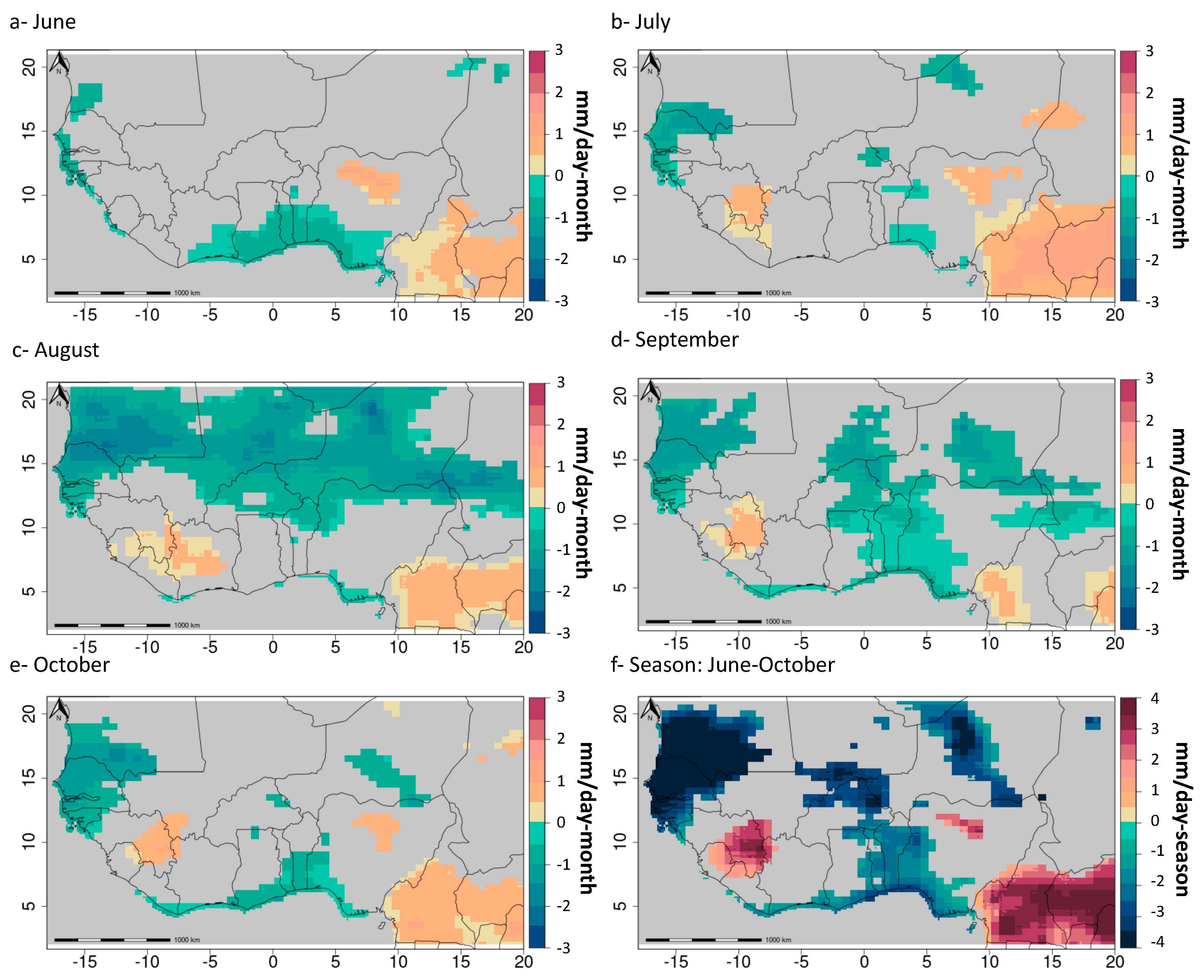
3.2. ET0
3.3. ET0 and Precipitation
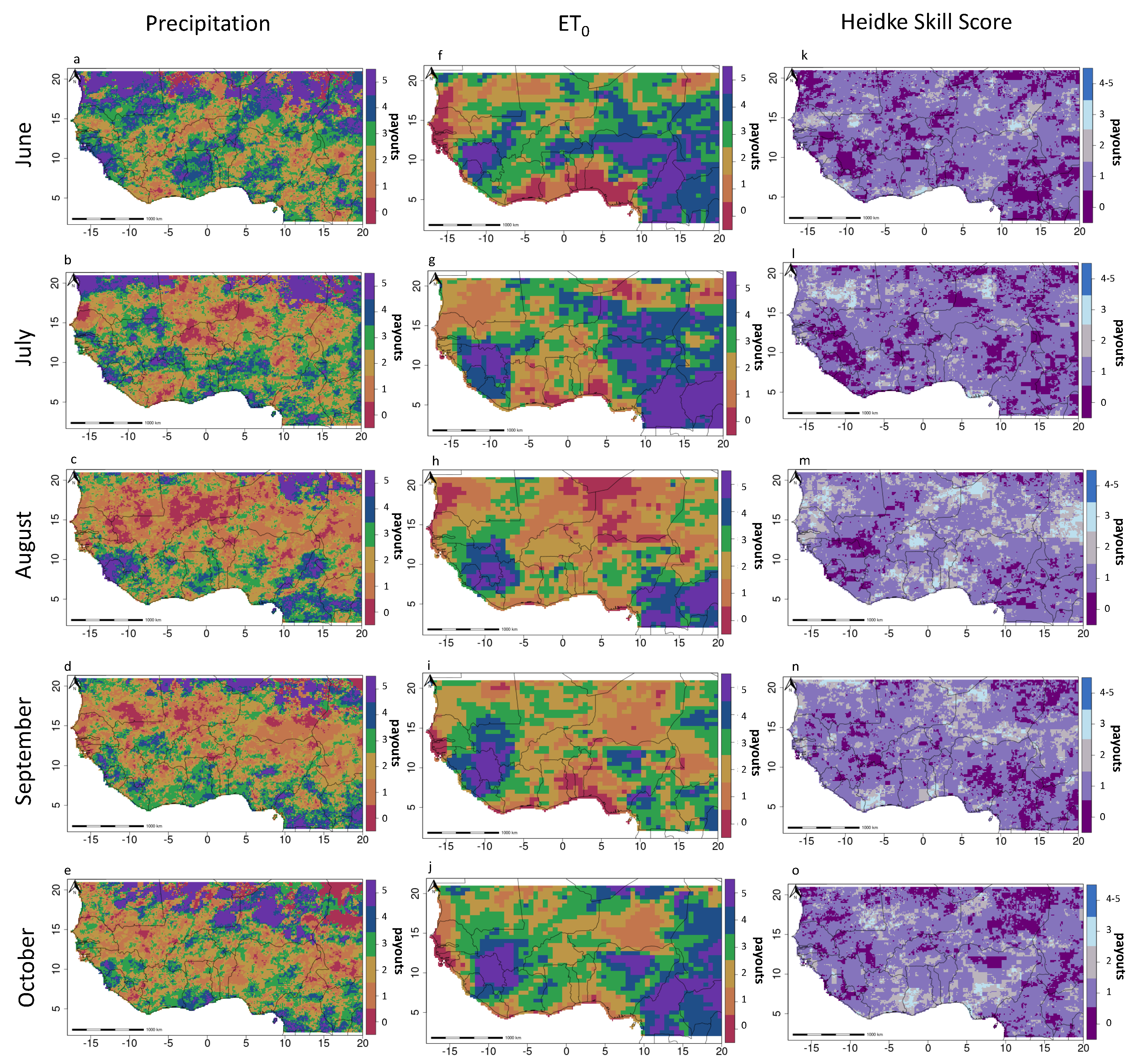
3.4. Indices and Heidke Skill Score
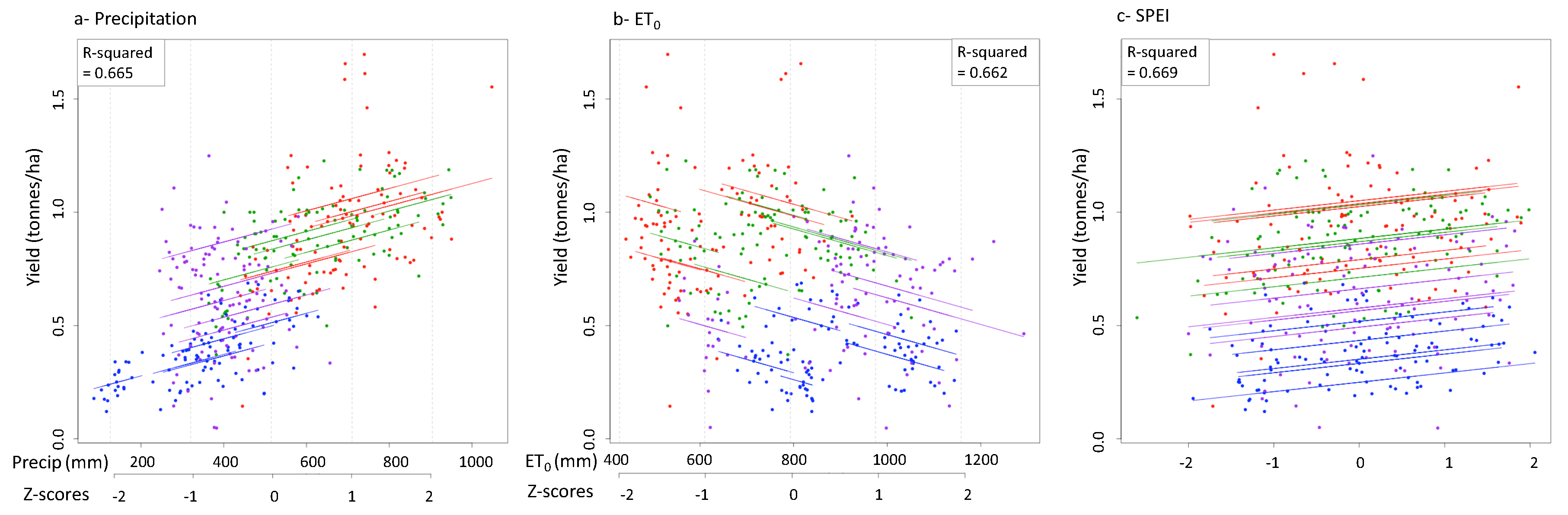
3.5. Linear Fits with Yield, Precipitation, ET0, and Spei
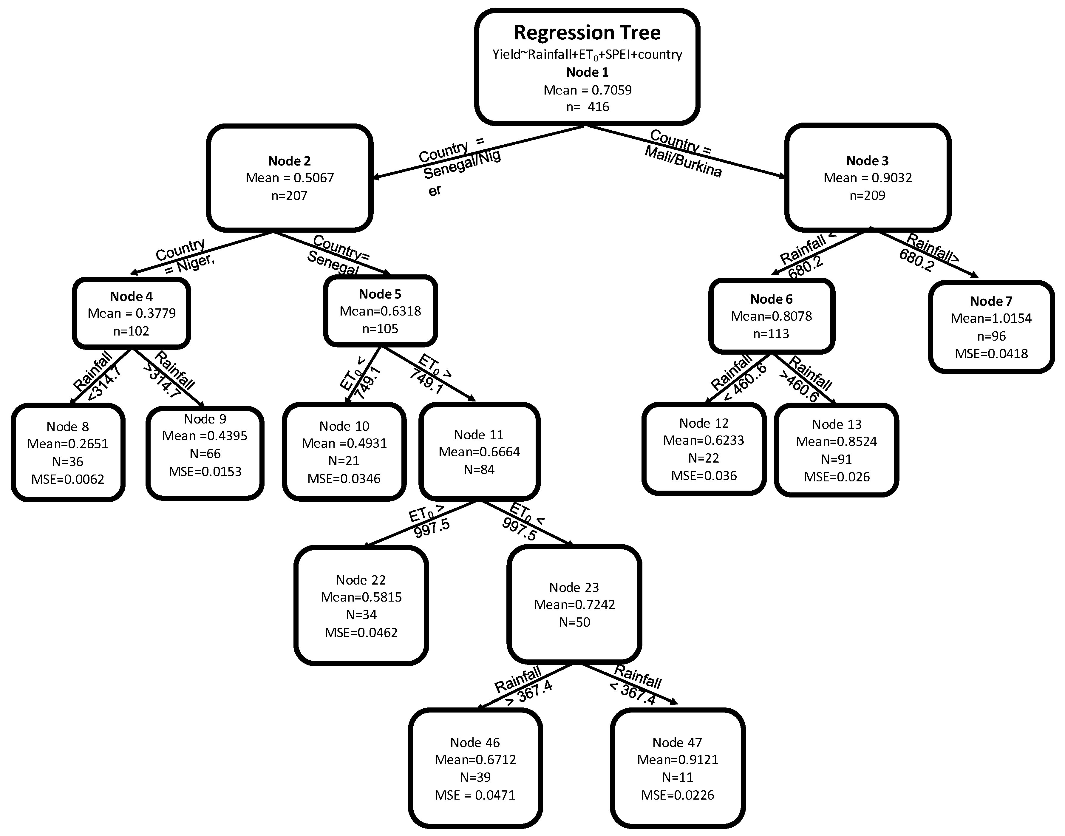
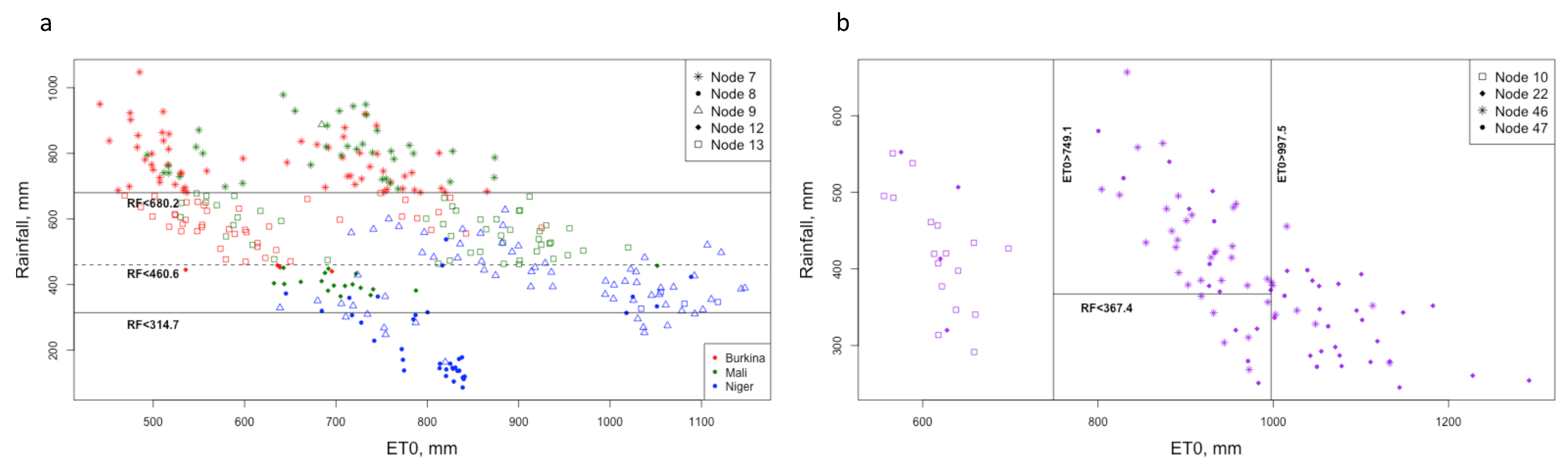
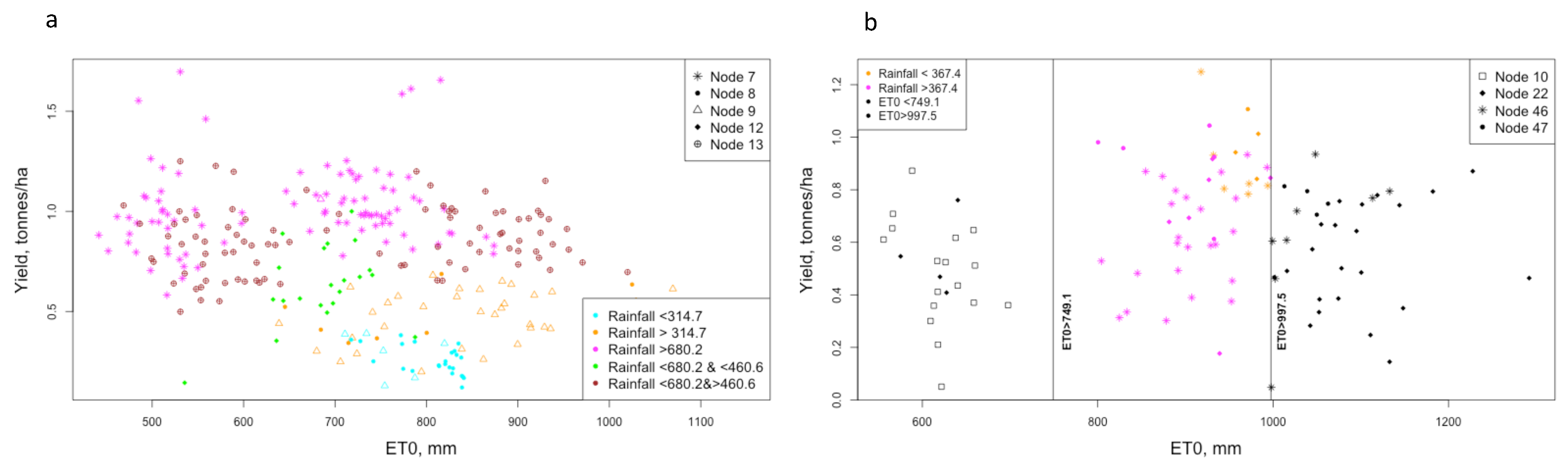
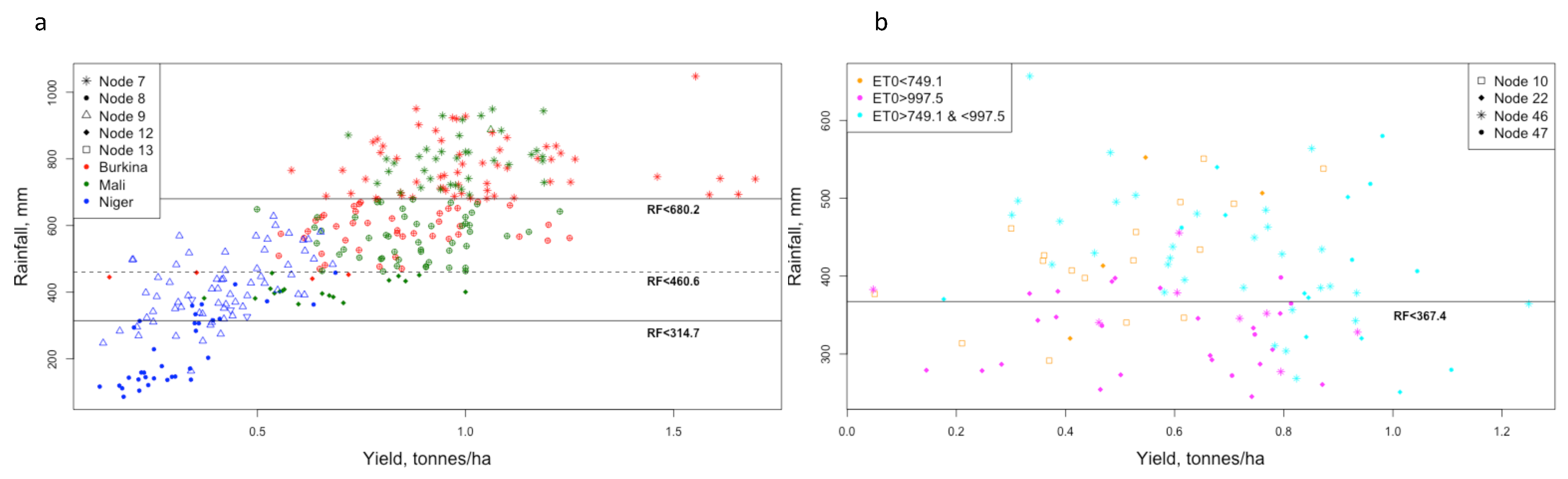
3.6. Regression Tree Analysis of Crop Yield
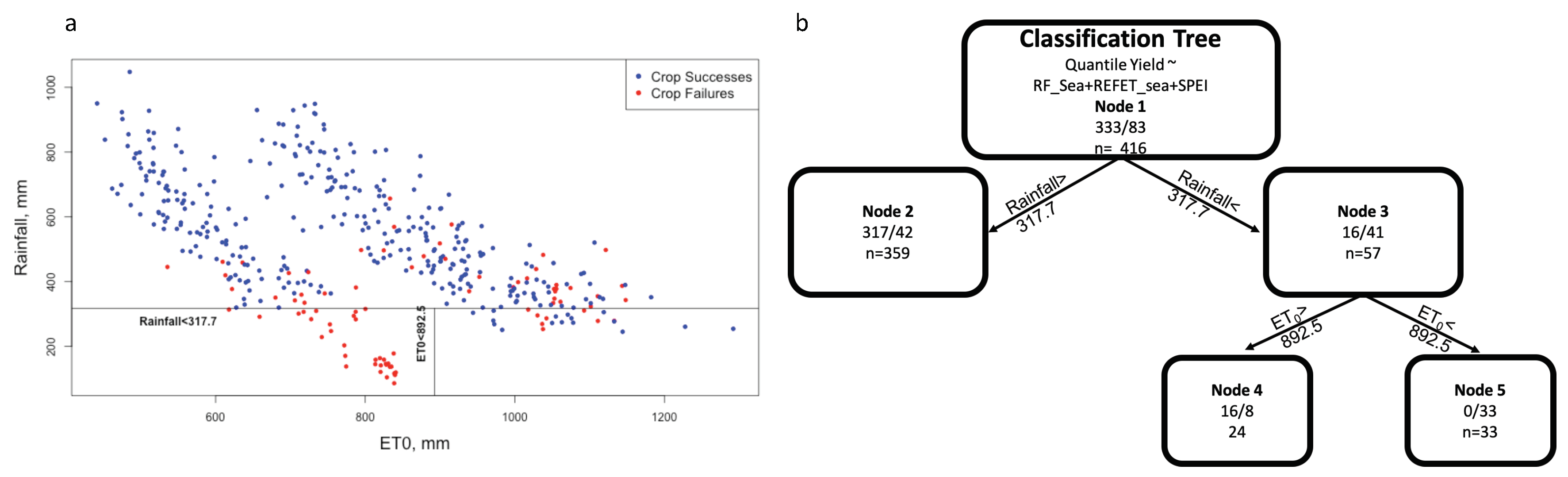
3.7. Classification Tree Analysis of Low Yield Years
4. Discussion
4.1. Precipitation Trends
4.2. ET0 Trends
4.3. Precipitation and ET0
4.4. Indices and Heidke Skill Score
4.5. Linear Fit of Yield with Precipitation, ET0, and Spei
4.6. Regression Tree
4.7. Classification Tree
5. Conclusions
Author Contributions
Funding
Acknowledgments
Conflicts of Interest
Appendix A
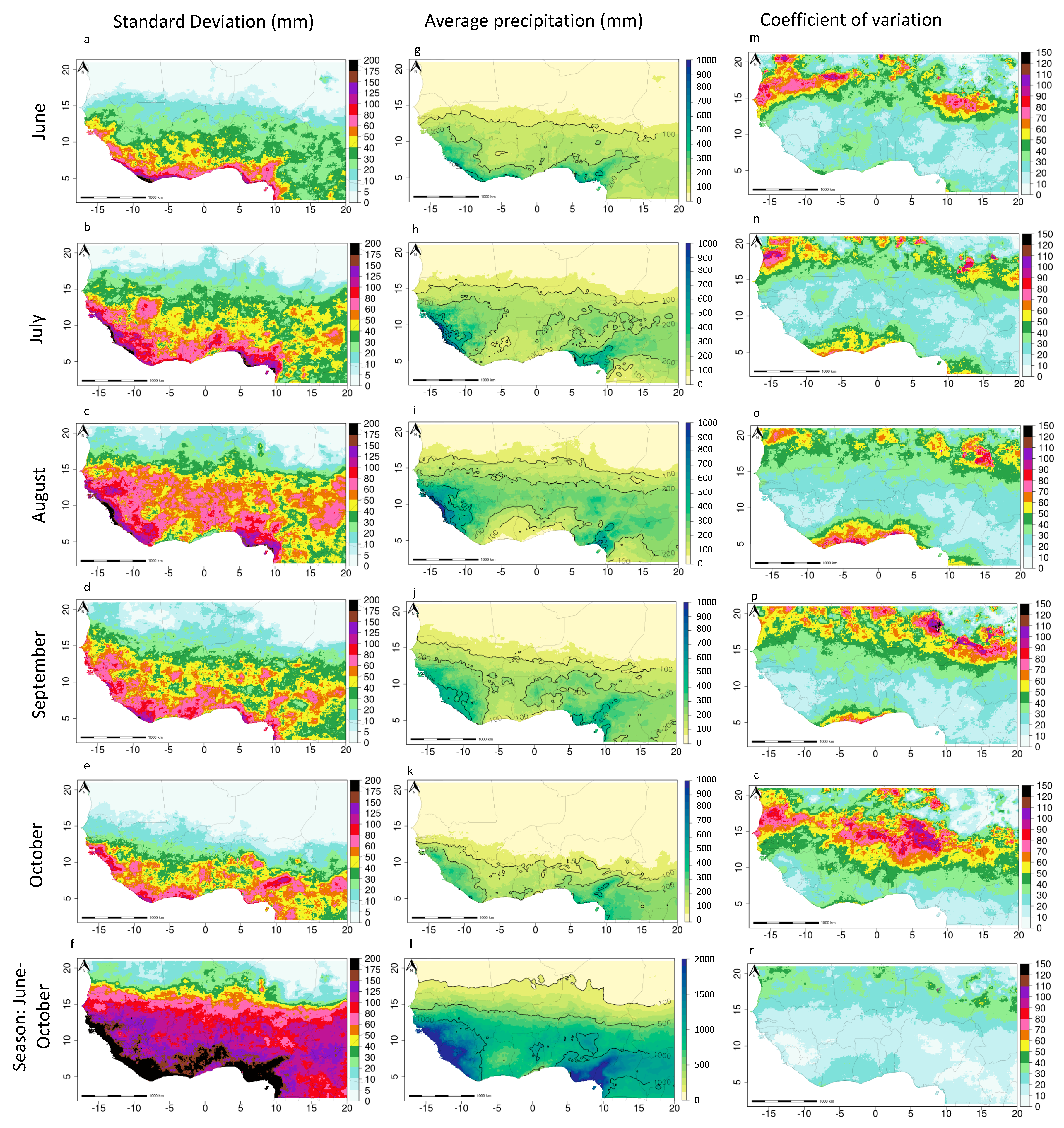
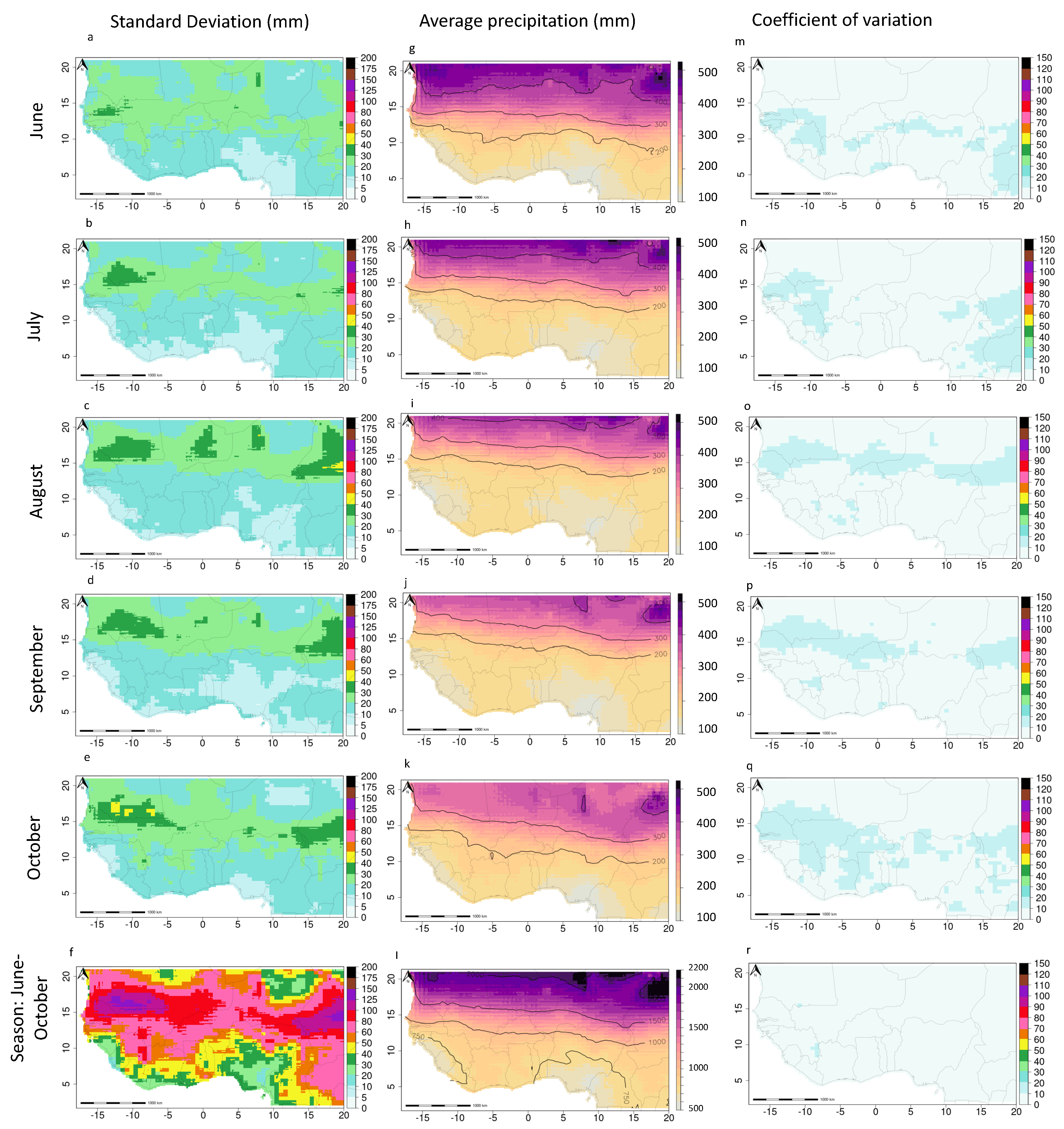
Appendix A.1. Standard Deviation and Coefficient of Variation for Precipitation and ET0


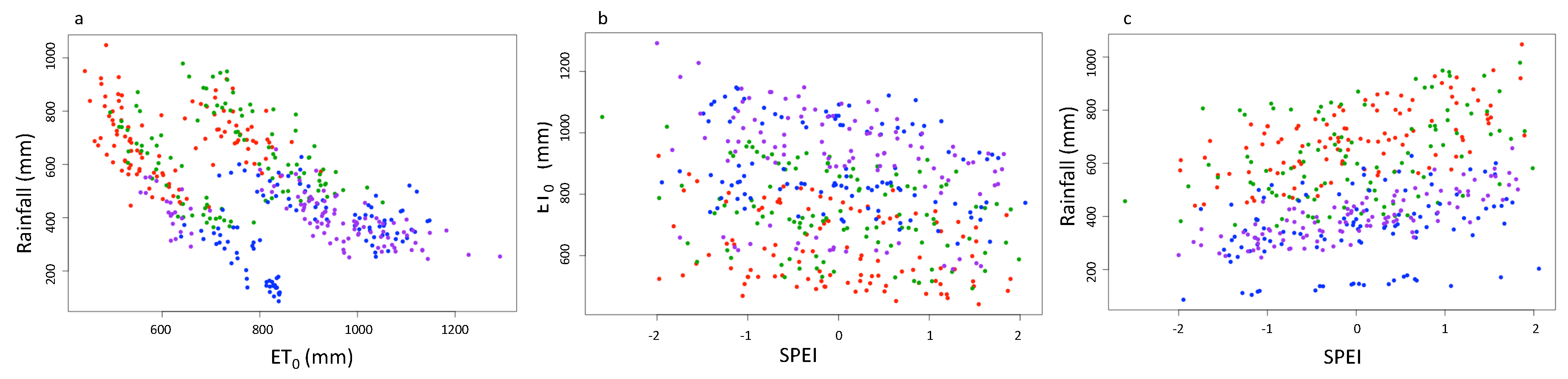
Appendix A.2. ET0 Precipitation and Spei Relationships

Appendix A.3. Specification Testing for Yield Regressions
F-Test

| Precipitation | Degrees of Freedom | Sum of Squares | F-statistic | Pr(>F) |
| Model 1, Model 2 | 19 | 7.45 | 12.85 | <2.2 × 10⁻¹⁶ *** |
| Model 2, Model 3 | 19 | 0.77 | 1.34 | 0.15 |
| Model 1, Model 3 | 38 | 8.21 | 7.21 | 2.2 × 10⁻¹⁶ *** |
| ET0 | Degrees of Freedom | Sum of Squares | F-statistic | Pr(>F) |
| Model 1, Model 2 | 19 | 21.44 | 36.71 | <2.2 × 10⁻¹⁶ *** |
| Model 2, Model 3 | 19 | 0.53 | 0.90 | 0.58 |
| Model 1, Model 3 | 38 | 8.21 | 7.21 | 2.2 × 10⁻¹⁶ *** |
| SPEI | Degrees of Freedom | Sum of Squares | F-statistic | Pr(>F) |
| Model 1, Model 2 | 19 | 25.28 | 44.21 | <2.2 × 10⁻¹⁶ *** |
| Model 2, Model 3 | 19 | 0.56 | 0.97 | 0.49 |
| Model 1, Model 3 | 38 | 25.83 | 22.53 | <2.2 × 10⁻¹⁶ *** |
Appendix A.4. Yield Analysis

Yield Regressions
| Burkina Faso | ||
| Estimate | pr(>t) | |
| Intercept | −15.74 | 0.057 |
| (8.19) | ||
| Slope | 0.008 | 0.044 * |
| (0.004) | ||
| Adjusted R-squared | 0.029 | |
| F-statistic | 4.15 | |
| p-value | 0.04 | |
| Mali | ||
| Estimate | pr(>t) | |
| Intercept | −10.41 | 0.072 |
| (5.72) | ||
| Slope | 0.006 | 0.051 |
| (0.003) | ||
| Adjusted R-squared | 0.027 | |
| F-statistic | 3.89 | |
| p-value | 0.051 | |
| Niger | ||
| Estimate | pr(>t) | |
| Intercept | −19.5 | 8.55 × 10⁻⁵ *** |
| (4.15) | ||
| Slope | 0.01 | 5.93 × 10⁻⁶ *** |
| (0.002) | ||
| Adjusted R-squared | 0.178 | |
| F-statistic | 22.89 | |
| p-value | 5.93 × 10⁻⁶ | |
| Senegal | ||
| Estimate | pr(>t) | |
| Intercept | −20.94 | 5.00 × 10⁻³ *** |
| (7.37) | ||
| Slope | 0.011 | 4.00 × 10⁻³ *** |
| (0.004) | ||
| Adjusted R-squared | 0.068 | |
| F-statistic | 8.58 | |
| p-value | 4.00 × 10⁻³ |
Appendix A.5. One-Way Anova Results for Linear Fit for Yield with Precipitation, ET0, and Spei
Appendix A.5.1. One-Way ANOVA Precipitation
| Degrees of Freedom | Sum of Squares | Mean Square | F-Value | Pr(F) | |
|---|---|---|---|---|---|
| Precipitation | 1 | 18.26 | 18.26 | 599 | <2.2 × 10⁻¹⁶ *** |
| Country | 19 | 7.45 | 0.39 | 12.9 | <2.2 × 10⁻¹⁶ *** |
| Residuals | 395 | 12.04 | 0.03 |
Appendix A.5.2. One-Way ANOVA ET0
| Degrees of Freedom | Sum of Squares | Mean Square | F-Value | Pr(F) | |
|---|---|---|---|---|---|
| ET0 | 1 | 4.17 | 4.17 | 135.54 | <2.2 × 10⁻¹⁶ *** |
| Country | 19 | 21.44 | 1.13 | 36.71 | <2.2 × 10⁻¹⁶ *** |
| Residuals | 395 | 12.14 | 0.03 |
Appendix A.5.3. One-Way ANOVA SPEI
| Degrees of Freedom | Sum of Squares | Mean Square | F-Value | Pr(F) | |
|---|---|---|---|---|---|
| ET0 | 1 | 0.59 | 0.59 | 19.53 | <1.28 × 10⁻⁵ *** |
| Country | 19 | 25.28 | 1.33 | 44.21 | <2.2 × 10⁻¹⁶ *** |
| Residuals | 395 | 11.89 | 0.03 |
References
- Cole, S.; Giné, X.; Tobacman, J.; Topalova, P.; Townsend, R.; Vickery, J. Barriers to household risk management: Evidence from India. Am. Econ. J. Appl. Econ. 2013, 5, 104–135. [Google Scholar] [CrossRef]
- Marteau, R.; Sultan, B.; Moron, V.; Alhassane, A.; Baron, C.; Traoré, S.B. The onset of the rainy season and farmers’ sowing strategy for pearl millet cultivation in Southwest Niger. Agric. For. Meteorol. 2011, 151, 1356–1369. [Google Scholar] [CrossRef]
- Barrett, C. Covariate Catastropic Risk Management in the Developing World: Discussion. Am. J. Agric. Econ. 2011, 93, 512–513. [Google Scholar] [CrossRef]
- Regional Overview of Food Insecurity Africa: African Food Security Prospects Brighter than Ever; Technical Report; FAO: Rome, Italy, 2015.
- Barrett, C.B.; Barnett, B.J.; Carter, M.R.; Chantarat, S.; Hansen, J.W.; Mude, A.G.; Osgood, D.; Skees, J.R.; Turvey, C.G.; Ward, M.N. Poverty Traps and Climate Risk: Limitations and Opportunities of Index-Based Risk Financing; International Research Institute for Climate and Society: New York, NY, USA, 2007. [Google Scholar]
- Matlon, P.J. Farmer risk management strategies: The case of the West African semi-arid tropics. In Risk in Agriculrure: Proceeding of the Tenth Agriculture Sector Symposium; The World Bank: Washington, DC, USA, 1991. [Google Scholar]
- Lin, B.B. Resilience in agriculture through crop diversification: Adaptive management for environmental change. BioScience 2011, 61, 183–193. [Google Scholar] [CrossRef]
- Xoconostle-Cázares, B.; Ramirez-Ortega, F.A.; Flores-Elenes, L.; Ruiz-Medrano, R. Drought tolerance in crop plants. Am. J. Plant. Physiol. 2010, 5, 1–16. [Google Scholar]
- Evenson, R.E.; Gollin, D. Assessing the impact of the Green Revolution, 1960 to 2000. Science 2003, 300, 758–762. [Google Scholar] [CrossRef]
- Vohland, K.; Barry, B. A review of in situ rainwater harvesting (RWH) practices modifying landscape functions in African drylands. Agric. Ecosyst. Environ. 2009, 131, 119–127. [Google Scholar] [CrossRef]
- Hellmuth, M.; Osgood, D.; Hess, U.; Moorhead, A.; Bhojwani, H. Index Insurance and Climate Risk: Prospoects for Development and Disaster Management; Climate and Society No. 2; WCAS: New York, NY, USA, 2009. [Google Scholar]
- Remote Sensing for Index Insurance, An Overview of Findings and Lessons Learned for Smallholder Agriculture, Report; Technical Report; International Fund of Agricultural Development: Rome, Italy, 2017.
- Madajewicz, M.; Tsegay, H.; Norton, M. Managing Risks to Agricultural Livelihoods: Impact Evaluation of the Harita Progam in Tigray, 2009–2012; Oxfam: Boston, MA, USA, 2013. [Google Scholar]
- Funk, C.C.; Brown, M.E. Declining global per capita agricultural production and warming oceans threaten food security. Food Secur. 2009, 1, 271–289. [Google Scholar] [CrossRef]
- R4 Rural Resilience Initiative, Annual Report: January–December 2018. Technical Report, World Food Programme. 2018. Available online: https://docs.wfp.org/api/documents/WFP-0000104178/download/ (accessed on 28 April 2020).
- PlaNet Guarantee: Benin, Burkina Faso, Mali, Senegal. Global Index Insurance Facility (GIIF) Partner Profile; Technical Report; World Bank: Washington, DC, USA, 2017; (In English). Available online: http://documents.worldbank.org/curated/en/787441490703399516/PlaNet-guarantee-Benin-Burkina-Faso-Mali-Senegal (accessed on 28 April 2020).
- Assurance Agricole Basee sur un Indice Climatique au Senegal; Technical Report; Global Index Insurance Fund (GIIF), World Bank Group: Washington, DC, USA, 2018; Available online: https://www.indexinsuranceforum.org/sites/default/files/19677_SenegalConference_4pager_FRE_final_%20March%2018.pdf (accessed on 28 April 2020).
- African Risk Capacity Funds Assisted at Least 2.1 Million People Affected by Drought; Technical Report; African Risk Capacity: Rome, Italy, 2018. Available online: https://www.africanriskcapacity.org/wp-content/uploads/2018/05/Payouts-and-Successes_2018_EN.pdf (accessed on 28 April 2020).
- Coleman, E.; Dick, W.; Gilliams, S.; Piccard, I.; Rispoli, F.; Stoppa, A. Remote Sensing for Index Insurance, Findings and Lessons Learned for Smallholder Agriculture; Technical Report; International Fund of Agricultural Development (IFAD): Rome, Italy, 2018; Available online: https://www.ifad.org/documents/38714170/39144386/RemoteSensing_LongGuide_2017.pdf/f2d22adb-c3b0-4fe3-9cbb-c25054d756fe (accessed on 28 April 2020).
- Cook, K.H.; Vizy, E.K. Impact of climate change on mid-twenty-first century growing seasons in Africa. Clim. Dyn. 2012, 39, 2937–2955. [Google Scholar] [CrossRef]
- Cornforth, R. Overview of the West African monsoon 2011. Weather 2012, 67, 59–65. [Google Scholar] [CrossRef]
- Nicholson, S.E.; Some, B.; Kone, B. An analysis of recent rainfall conditions in West Africa, including the rainy seasons of the 1997 El Niño and the 1998 La Niña years. J. Clim. 2000, 13, 2628–2640. [Google Scholar] [CrossRef]
- Nicholson, S. On the question of the recovery of the rains in the West African Sahel. J. Arid. Environ. 2005, 63, 615–641. [Google Scholar] [CrossRef]
- Nicholson, S.E. The West African Sahel: A review of recent studies on the rainfall regime and its interannual variability. Isrn Meteorol. 2013, 2013, 453521. [Google Scholar] [CrossRef]
- Hayward, D.; Oguntoyinbo, J.S. Climatology of West Africa; Science: London, UK, 1987. [Google Scholar]
- Funk, C.; Peterson, P.; Landsfeld, M.; Pedreros, D.; Verdin, J.; Shukla, S.; Husak, G.; Rowland, J.; Harrison, L.; Hoell, A.; et al. The climate hazards infrared precipitation with stations—A new environmental record for monitoring extremes. Sci. Data 2015, 2, 1–21. [Google Scholar] [CrossRef] [PubMed]
- Hobbins, M.; Harrison, L.; Blakeley, S.L.; Dewes, C.; Husak, G.J.; Shukla, S.; Jayanthi, H.; McNally, A.; Sarmiento, D.; Verdin, J. Drought in Africa: Understanding and Exploiting the Demand Perspective Using a New Evaporative Demand Reanalysis. AGUFM 2018, 2018, GC21D-1121. [Google Scholar]
- Hobbins, M.; Dewes, C.; Jayanthi, H.; McNally, A.; Sarmiento, D.; Shukla, S.; Verdin, J. Developing and exploiting a new global reanalysis of evaporative demand for global food-security assessments and drought monitoring. In Proceedings of the American Meteorological Society Annual Meeting, Phoenix, AZ, USA, 6–10 January 2019. [Google Scholar]
- Rodrigues, L.R.L.; García-Serrano, J.; Doblas-Reyes, F. Seasonal forecast quality of the West African monsoon rainfall regimes by multiple forecast systems. J. Geophys. Res. Atmos. 2014, 119, 7908–7930. [Google Scholar] [CrossRef]
- Giannini, A.; Saravanan, R.; Chang, P. Oceanic forcing of Sahel rainfall on interannual to interdecadal time scales. Science 2003, 302, 1027–1030. [Google Scholar] [CrossRef]
- Biasutti, M.; Sobel, A.H. Delayed Sahel rainfall and global seasonal cycle in a warmer climate. Geophys. Res. Lett. 2009, 36, 23. [Google Scholar] [CrossRef]
- Biasutti, M. Forced Sahel rainfall trends in the CMIP5 archive. J. Geophys. Res. Atmos. 2013, 118, 1613–1623. [Google Scholar] [CrossRef]
- Allen, R.G.; Pereira, L.S.; Raes, D.; Smith, M. Crop Evapotranspiration-Guidelines for Computing Crop Water Requirements; FAO Irrigation and Drainage Paper 56; FAO: Rome, Italy, 1998; Volume 300, p. D05109. [Google Scholar]
- Hobbins, M.T.; Wood, A.; McEvoy, D.J.; Huntington, J.L.; Morton, C.; Anderson, M.; Hain, C. The evaporative demand drought index. Part I: Linking drought evolution to variations in evaporative demand. J. Hydrometeorol. 2016, 17, 1745–1761. [Google Scholar] [CrossRef]
- Peng, L.; Li, Y.; Feng, H. The best alternative for estimating reference crop evapotranspiration in different sub-regions of mainland China. Sci. Rep. 2017, 7, 5458. [Google Scholar] [CrossRef] [PubMed]
- Sultan, B.; Roudier, P.; Quirion, P.; Alhassane, A.; Muller, B.; Dingkuhn, M.; Ciais, P.; Guimberteau, M.; Traore, S.; Baron, C. Assessing climate change impacts on sorghum and millet yields in the Sudanian and Sahelian savannas of West Africa. Environ. Res. Lett. 2013, 8, 014040. [Google Scholar] [CrossRef]
- Prasad, P.; Staggenborg, S.; Ristic, Z. Impacts of drought and/or heat stress on physiological, developmental, growth, and yield processes of crop plants. In Response of Crops to Limited Water: Understanding and Modeling Water Stress Effects on Plant Growth Processes; American Society of Agronomy: Madison, WI, USA, 2008; pp. 301–355. [Google Scholar]
- Wheeler, T.R.; Craufurd, P.Q.; Ellis, R.H.; Porter, J.R.; Prasad, P.V. Temperature variability and the yield of annual crops. Agric. Ecosyst. Environ. 2000, 82, 159–167. [Google Scholar] [CrossRef]
- Field, C.B. Climate Change 2014—Impacts, Adaptation and Vulnerability: Regional Aspects; Cambridge University Press: Cambridge, UK, 2014. [Google Scholar]
- Estes, L.D.; Chaney, N.W.; Herrera-Estrada, J.; Sheffield, J.; Caylor, K.K.; Wood, E.F. Changing water availability during the African maize-growing season, 1979–2010. Environ. Res. Lett. 2014, 9, 075005. [Google Scholar] [CrossRef]
- R4 Rural Resilience Initiative: Quarterly Report, July–September 2016; Technical Report; World Food Programme: Rome, Italy, 2016.
- Svoboda, M.; Fuchs, B. Handbook of Drought Indicators and Indices; Integrated Drought Management Tools and Guidelines Series 2, Geneva; World Meteorological Organization and Global Water Partnership: Geneva, Switzerland, 2016. [Google Scholar]
- Hobbins, M.; McNally, A.; Sarmiento, D.; Jansma, T.; Husak, G.; Turner, W.; Verdin, J. Using a New Evaporative Demand Reanalysis to Understand the Demand Perspective of Drought and Food Insecurity in Africa. In Proceedings of the 100th American Meteorological Society Annual Meeting, Boston, MA, USA, 12–16 January 2020. [Google Scholar]
- Hobbins, M.; McNally, A.; Sarmiento, D.; Verdin, J. Drought in Africa: Understanding and Exploiting the Demand Perspective Using A New Evaporative Demand Reanalysis. In Proceedings of the European Meteorological Society Annual Meeting, Copenhagen, Denmark, 9–13 September 2019. [Google Scholar]
- Allen, R.G.; Clemmens, A.J.; Burt, C.M.; Solomon, K.; O’Halloran, T. Prediction accuracy for projectwide evapotranspiration using crop coefficients and reference evapotranspiration. J. Irrig. Drain. Eng. 2005, 131, 24–36. [Google Scholar] [CrossRef]
- Gelaro, R.; McCarty, W.; Suárez, M.J.; Todling, R.; Molod, A.; Takacs, L.; Randles, C.A.; Darmenov, A.; Bosilovich, M.G.; Reichle, R.; et al. The modern-era retrospective analysis for research and applications, version 2 (MERRA-2). J. Clim. 2017, 30, 5419–5454. [Google Scholar] [CrossRef]
- Vicente-Serrano, S.M.; Beguería, S.; López-Moreno, J.I.; Angulo, M.; El Kenawy, A. A new global 0.5 gridded dataset (1901–2006) of a multiscalar drought index: Comparison with current drought index datasets based on the Palmer Drought Severity Index. J. Hydrometeorol. 2010, 11, 1033–1043. [Google Scholar] [CrossRef]
- Vicente-Serrano, S.M.; Beguería, S.; López-Moreno, J.I. A multiscalar drought index sensitive to global warming: The standardized precipitation evapotranspiration index. J. Clim. 2010, 23, 1696–1718. [Google Scholar] [CrossRef]
- De Leeuw, J.; Vrieling, A.; Shee, A.; Atzberger, C.; Hadgu, K.M.; Biradar, C.M.; Keah, H.; Turvey, C. The potential and uptake of remote sensing in insurance: A review. Remote Sens. 2014, 6, 10888–10912. [Google Scholar] [CrossRef]
- Norton, M.; Osgood, D.; Madajewicz, M.; Holthaus, E.; Peterson, N.; Diro, R.; Mullally, C.; Teh, T.L.; Gebremichael, M. Evidence of demand for index insurance: Experimental games and commercial transactions in Ethiopia. J. Dev. Stud. 2014, 50, 630–648. [Google Scholar] [CrossRef]
- Barnston, A.G. Correspondence among the correlation, RMSE, and Heidke forecast verification measures, refinement of the Heidke score. Weather Forecast. 1992, 7, 699–709. [Google Scholar] [CrossRef]
- Jensen, N.; Stoeffler, Q.; Fava, F.; Vrieling, A.; Atzberger, C.; Meroni, M.; Mude, A.; Carter, M. Does the design matter? Comparing satellite-based indices for insuring pastoralists against drought. Ecol. Econ. 2019, 162, 59–73. [Google Scholar] [CrossRef]
- Wang, G.; Alo, C.A. Changes in precipitation seasonality in West Africa predicted by RegCM3 and the impact of dynamic vegetation feedback. Int. J. Geophys. 2012, 2012, 597205. [Google Scholar] [CrossRef]
- Zhang, W.; Brandt, M.; Guichard, F.; Tian, Q.; Fensholt, R. Using long-term daily satellite based rainfall data (1983–2015) to analyze spatio-temporal changes in the sahelian rainfall regime. J. Hydrol. 2017, 550, 427–440. [Google Scholar] [CrossRef]
- L’HOTE, Y.; Mahe, G.; Some, B. The 1990s rainfall in the Sahel: The third driest decade since the beginning of the century. Hydrol. Sci. J. 2003, 48, 493–496. [Google Scholar] [CrossRef]
- Nicholson, S.E.; Funk, C.; Fink, A.H. Rainfall over the African continent from the 19th through the 21st century. Glob. Planet. Chang. 2018, 165, 114–127. [Google Scholar] [CrossRef]
- Abiye, O.E.; Matthew, O.J.; Sunmonu, L.A.; Babatunde, O.A. Potential evapotranspiration trends in West Africa from 1906 to 2015. Appl. Sci. 2019, 1, 1434. [Google Scholar] [CrossRef]
- Marshall, M.; Funk, C.; Michaelsen, J. Examining evapotranspiration trends in Africa. Clim. Dyn. 2012, 38, 1849–1865. [Google Scholar] [CrossRef]
- R4 Rural Resilience Initiative Annual Report January–December 2018; Technical Report; World Food Programme: Rome, Italy, 2018.
- Collier, B.; Skees, J.; Barnett, B. Weather index insurance and climate change: Opportunities and challenges in lower income countries. Geneva Pap. Risk Insur. Issues Pract. 2009, 34, 401–424. [Google Scholar] [CrossRef]
- Shirley, K.; Osgood, D.; Robert, A.; Block, P.; Lall, U.; Hansen, J.; Kirshener, S.; Moron, V.; Ines, A.; TUrvey, C.; et al. Rainfall Modeling and Simulation. Paper Presented at a Workshop on ’Technical Issues in Index Insurance, IRI, Columbia University, New York, NY, USA, 7–8 October 2008; Available online: http://iri.columbia.edu/csp/issue2/workshop (accessed on 28 April 2020).
- Hoerling, M.; Hurrell, J.; Eischeid, J.; Phillips, A. Detection and attribution of twentieth-century northern and southern African rainfall change. J. Clim. 2006, 19, 3989–4008. [Google Scholar] [CrossRef]
- Zhang, R.; Delworth, T.L.; Sutton, R.; Hodson, D.L.; Dixon, K.W.; Held, I.M.; Kushnir, Y.; Marshall, J.; Ming, Y.; Msadek, R.; et al. Have aerosols caused the observed Atlantic multidecadal variability? J. Atmos. Sci. 2013, 70, 1135–1144. [Google Scholar] [CrossRef]
- Chantarat, S.; Mude, A.G.; Barrett, C.B.; Carter, M.R. Designing index-based livestock insurance for managing asset risk in northern Kenya. J. Risk Insur. 2013, 80, 205–237. [Google Scholar] [CrossRef]
- Klisch, A.; Atzberger, C. Operational drought monitoring in Kenya using MODIS NDVI time series. Remote Sens. 2016, 8, 267. [Google Scholar] [CrossRef]
- Louise, L.; Agnès, B.; Danny, L.S. Regional analysis of crop and natural vegetation in West Africa based on NDVI metrics. In Proceedings of the 2014 IEEE Geoscience and Remote Sensing Symposium, Quebec City, QC, Canada, 13–18 July 2014; pp. 5107–5110. [Google Scholar]
- Turvey, C.G.; Mclaurin, M.K. Applicability of the normalized difference vegetation index (NDVI) in index-based crop insurance design. Weather. Clim. Soc. 2012, 4, 271–284. [Google Scholar] [CrossRef]
- Meroni, M.; Fasbender, D.; Rembold, F.; Atzberger, C.; Klisch, A. Near real-time vegetation anomaly detection with MODIS NDVI: Timeliness vs. accuracy and effect of anomaly computation options. Remote Sens. Environ. 2019, 221, 508–521. [Google Scholar] [CrossRef]
- Husak, G.; Shukla, S.; Funk, C.; Hobbins, M. Investigating the Inputs to SPEI and Their Importance in Identifying Agroclimatic Hazards. In Proceedings of the AGU Fall Meeting Abstracts, Washington, DC, USA, 10–14 December 2018. [Google Scholar]


| Model 1: Precipitation | Model 2: ET0 | Model 3: SPEI | |
|---|---|---|---|
| Intercept | 0.4954 *** | 1.1026 *** | 0.7521 *** |
| (−0.0759) | (−0.1039) | (−0.0379) | |
| X1 | 0.0005 *** | −0.0006 *** | 0.2856 *** |
| (−0.0001) | (−0.0002) | (−0.0536) | |
| Burkina-Kenedougou | 0.1494 * | 0.2278 *** | 0.0385 *** |
| (−0.0634) | (− 0.0564) | (−0.0535) | |
| Burkina-Kouritenga | −0.0085 | −0.0046 | 0.0385 |
| (−0.0551) | (0.0554) | (−0.0535) | |
| Burkina-Mouhoun | 0.226 *** | 0.402 *** | 0.2988 *** |
| (−0.0568) | (0.0611) | (−0.0535) | |
| Burkina-Silassi | 0.1684 ** | 0.3503 *** | 0.2726 *** |
| (−0.0596) | (−0.0611) | (−0.0535) | |
| Mali-Kayes | 0.0436 | 0.0946 | 0.1179 * |
| (−0.057) | (−0.0544) | (−0.0535) | |
| Mali-Koulikoro | 0.0972 | 0.2928 *** | 0.1325 * |
| (−0.0546) | (−0.0699) | (−0.0535) | |
| Mali-Mopti | 0.0191 | 0.0131 | −0.0396 |
| (−0.0557) | (−0.056) | (−0.0535) | |
| Mali-Segou | 0.1347 * | 0.3019 *** | 0.1315 * |
| (−0.0539) | (−0.0716) | (−0.0535) | |
| Mali-Sikasso | 0.1265 | 0.3539 *** | 0.2808 *** |
| (−0.066) | (−0.0587) | (−0.0542) | |
| Niger-Bouza | −0.2407 *** | −0.0557 | −0.3178 |
| (−0.0571) | (−0.0902) | (−0.0535) | |
| Niger-Dosso | −0.2264 *** | −0.0975 | −0.2338 *** |
| (−0.05459) | (−0.0665) | (−0.0542) | |
| Niger-Filingue | −0.3094 *** | −0.3415 *** | −0.4191 *** |
| (−0.0602) | (−0.0582) | (−0.0535) | |
| Niger-Goure | −0.3062 *** | −0.3722 *** | −0.5024 *** |
| (−0.073) | (−0.0656) | (−0.0542) | |
| Niger-Mayahi | −0.3162 *** | −0.1432 | −0.4006 *** |
| (−0.0582) | (−0.0891) | (−0.0542) | |
| Senegal-Diourbel | −0.0719 | 0.1062 | −0.1752 ** |
| (−0.0596) | (−0.0945) | (−0.0535) | |
| Senegal-Fatick | −0.0092 | 0.1580 | −0.09 |
| (−0.0574) | (−0.0871) | (−0.0535) | |
| Senegal-Foundiougne | 0.1864 ** | 0.3092 *** | 0.1071 * |
| (−0.0573) | (−0.0776) | (−0.0535) | |
| Senegal-Gossas | −0.1458 ** | −0.0115 | −0.1868 *** |
| (−0.0549) | (−0.0725) | (−0.0535) | |
| Senegal-Mbacke | −0.2022 *** | −0.2458 *** | −0.2593 *** |
| (−0.0557) | (−0.0542) | (−0.0535) | |
| Adjusted R-squared | 0.6649 | 0.6784 | 0.6692 |
| F-statistic | 42.16 | 41.65 | 42.97 |
| Degrees of Freedom | 395 | 395 | 395 |
© 2020 by the authors. Licensee MDPI, Basel, Switzerland. This article is an open access article distributed under the terms and conditions of the Creative Commons Attribution (CC BY) license (http://creativecommons.org/licenses/by/4.0/).
Share and Cite
Blakeley, S.L.; Sweeney, S.; Husak, G.; Harrison, L.; Funk, C.; Peterson, P.; Osgood, D.E. Identifying Precipitation and Reference Evapotranspiration Trends in West Africa to Support Drought Insurance. Remote Sens. 2020, 12, 2432. https://doi.org/10.3390/rs12152432
Blakeley SL, Sweeney S, Husak G, Harrison L, Funk C, Peterson P, Osgood DE. Identifying Precipitation and Reference Evapotranspiration Trends in West Africa to Support Drought Insurance. Remote Sensing. 2020; 12(15):2432. https://doi.org/10.3390/rs12152432
Chicago/Turabian StyleBlakeley, S. Lucille, Stuart Sweeney, Gregory Husak, Laura Harrison, Chris Funk, Pete Peterson, and Daniel E. Osgood. 2020. "Identifying Precipitation and Reference Evapotranspiration Trends in West Africa to Support Drought Insurance" Remote Sensing 12, no. 15: 2432. https://doi.org/10.3390/rs12152432
APA StyleBlakeley, S. L., Sweeney, S., Husak, G., Harrison, L., Funk, C., Peterson, P., & Osgood, D. E. (2020). Identifying Precipitation and Reference Evapotranspiration Trends in West Africa to Support Drought Insurance. Remote Sensing, 12(15), 2432. https://doi.org/10.3390/rs12152432