Geo-Location Algorithm for Building Targets in Oblique Remote Sensing Images Based on Deep Learning and Height Estimation

Abstract

To improve the accuracy of the geographic positioning of a single aerial remote sensing image, the height information of a building in the image must be considered. Oblique remote sensing images are essentially two-dimensional images and produce a large positioning error if a traditional positioning algorithm is used to locate the building directly. To address this problem, this study uses a convolutional neural network to automatically detect the location of buildings in remote sensing images. Moreover, it optimizes an automatic building recognition algorithm for oblique aerial remote sensing images based on You Only Look Once V4 (YOLO V4). This study also proposes a positioning algorithm for the building target, which uses the imaging angle to estimate the height of a building, and combines the spatial coordinate transformation matrix to calculate high-accuracy geo-location of target buildings. Simulation analysis shows that the traditional positioning algorithm inevitably leads to large errors in the positioning of building targets. When the target height is 50 m and the imaging angle is 70°, the positioning error is 114.89 m. Flight tests show that the algorithm established in this study can improve the positioning accuracy of building targets by approximately 20%–50% depending on the difference in target height.

1. Introduction

To realize remote sensing photogrammetry, various photoelectric sensors have been carried out on aircrafts to obtain ground images. Obtaining the location information of the target in the image using a geo-location algorithm is a research hotspot in recent years [1,2,3]. Currently, research on target positioning algorithms focuses on improving the positioning accuracy of ground targets, implying that the positioning error caused by the building height is rarely considered in the algorithm.

Obtaining high-accuracy geo-location of building targets in real time requires automatic detection of buildings in remote sensing images and an appropriate method to calculate the height of buildings from the image. Traditional aerial photogrammetry uses vertical overlook (i.e., nadir) imaging and uses an airborne camera to obtain a large-scale two-dimensional (2D) image of the city. On this basis, most research on building detection algorithms also aims at overlooking remote sensing images. Owing to the differences in buildings in an image, semantic analysis and image segmentation are used for automatic detection. A single overlooking remote sensing image can contain a large number of buildings. With the development of aerial photoelectric loads, such as airborne cameras and photoelectric pods, long-distance oblique imaging has become a major method for obtaining aerial remote sensing images. Unlike overlooking imaging, oblique imaging can better describe specific details of urban buildings, which is conducive to 3D modeling, map marking, and other works [4]. To achieve these goals, a high-accuracy geo-location of urban building targets should be realized. Scholars have conducted extensive research on target geo-location algorithms. To locate the target with a single image, an earth ellipsoid model is widely used in the positioning process. For example, Stich proposed a target positioning algorithm based on the earth ellipsoid model; this realizes the passive positioning of the ground target from a single image by using an aerial camera and reduces the influence of the earth’s curvature on the positioning result [5]. The Global Hawk unmanned aerial vehicle (UAV) positioning system is also based on an earth ellipsoid model to calculate the geodetic coordinates of the image center [6]. To improve the positioning accuracy, scholars have optimized the algorithm by using multiple measurements and adding auxiliary information [7,8,9]. L.G. Tan proposed the pixel sight vector method through the parameters of the laser range finder (LRF) and angle sensors, establishing a multi-target positioning model that improves the accuracy of the positioning algorithm. Similarly, N. Merkle used the information provided by the synthetic aperture radar (SAR) to achieve high-accuracy positioning of targets. Considering a problem wherein single UAV positioning is significantly affected by random errors, various multi-UAV measurement systems have been established to reduce random errors [10,11,12,13]. G. Bai and Y. Qu proposed cooperative positioning models for double UAVs and multi-UAVs, respectively. Many scholars used filtering algorithms to locate targets. For example, the target positioning algorithm based on Kalman filtering proposed by H.R. Hosseinpoor improves the accuracy of target positioning through multiple measurements. This filtering-based positioning algorithm is widely used in target tracking [14].

Although extensive research has been conducted on positioning algorithms, only a few analyzed the positioning error caused by the target height. A remote sensing image is obtained by projecting the target area on a sensor that receives the photoelectric signal. The sensor is usually a charge-coupled device (CCD). The essence of an aerial remote sensing image is a 2D image, resulting in a traditional positioning algorithm that cannot calculate the height of the building in the image. C. Qiao considered the influence of elevation information on the positioning results and relied on digital elevation model (DEM) data, instead of the earth ellipsoid model, which resolved the elevation error of ground targets [15,16]. However, the DEM data do not contain the elevation information of the building and, thus, cannot resolve the large positioning error of the building target. Some algorithms, based on LRFs, for obtaining distance information can locate building targets. However, the positioning result is significantly affected by the ranging accuracy, and most airborne LRF has a limited working range (within 20 km). To obtain a large range for remote sensing images, the shooting distance of long-distance oblique remote sensing images is usually more than 30 km. Therefore, this algorithm cannot meet the requirements of high-accuracy positioning of building targets. Manual building identification and calculation by downloading the aerial remote sensing image results in poor timeliness of the data, and it cannot meet the requirements of obtaining the target’s geo-location in real time.

This study aims to address the problem of large positioning error of building targets and establishes a building target positioning algorithm that can be widely used in oblique remote sensing images. The remainder of this paper is organized as follows. Section 2 optimizes the YOLO v4 convolutional neural network based on deep learning theory and characteristics of building remote sensing images and realizes the automatic detection of buildings in various squint remote sensing images. Section 3 calculates the building height in the image based on the angle information and proposes a high-precision positioning algorithm for the building target. Section 4 proves the importance and effectiveness of the algorithm through simulation analysis and actual flight tests. Finally, Section 5 summarizes this study.

2. Automatic Building Detection Algorithm for Oblique Remote Sensing Images

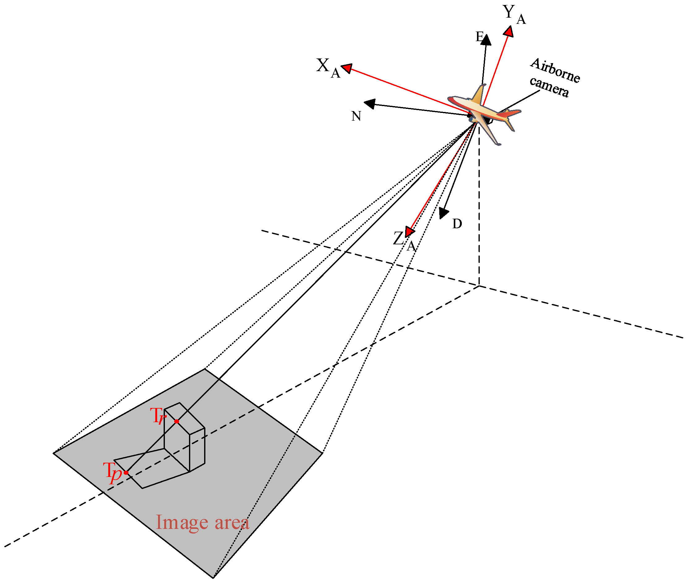
As mentioned previously, the essence of aerial remote sensing images is 2D images. The principle of the traditional target positioning algorithm is calculated by the intersection of the collinear equation composed of the projected pixel points, camera main point, and earth ellipsoid equation or DEM model. Therefore, when locating a building target, the actual positioning result is the ground position blocked by the building, as shown in Figure 1. In the figure, $T_r$ is the actual position of the target point, and $T_P$ is the calculation result of the traditional positioning algorithm.

An appropriate method that can detect the image and automatically identify the building should be selected to distinguish the building target in the image from the ground target to avoid affecting the positioning result of the ground target. The buildings in the oblique images show different characteristics from those of the overlooking images, such as neighboring buildings being blocked in the image. The height, shadow, angle, and edge characteristics vary for each building. Therefore, the traditional top-down image recognition method is less effective and cannot detect buildings in oblique images. Recently, owing to the rapid development of deep learning algorithms based on convolutional neural networks, scholars have conducted research on the building detection in remote sensing images through deep learning. However, most research focused on the detection of targets from overlooking images, especially for the automatic recognition of large-scale urban images [17,18]. The relevant research results cannot be directly applied to oblique images. Therefore, although the application of long-range oblique imaging is widely used, limited research has been conducted on related datasets and detection algorithms.

YOLO is a mature open-source target detection algorithm with the advantages of high accuracy, small volume, and fast operation speed [19,20,21,22]. Its advantages and characteristics perfectly match the requirements of aerial remote sensing images. Aerial oblique images are usually captured using airborne cameras or photoelectric pods carried by an aircraft, requiring real-time image processing and high recognition accuracy. The computing power of aerial cameras is limited, so the operation speed requirement of the algorithm is also high. This study uses YOLO v4 as the basis and optimizes it to achieve the automatic detection of buildings from telephoto oblique remote sensing images.

Figure 2 clearly describes the neural network structure of the building detection algorithm. CBL is the most basic component of the neural network, consisting of a convolutional (Conv) layer, a batch normalization (BN) layer, and a leaky rectified linear unit (ReLU) activation function. In the CBM, the Mish activation function is used to replace the leaky ReLU activation function. Moreover, a Res unit exists to construct a deeper network. The CSP(n) consists of three convolutional layers and n Res unit modules. The SPP module is used to achieve multiscale integration. It uses four scales of 1 × 1, 5 × 5, 9 × 9, and 13 × 13 for maximum pooling [22].

Training the neural network through a large amount of data is required to realize the automatic detection of buildings. However, existing public datasets do not have high-quality data for oblique aerial building images. A telephoto oblique aerial camera usually adopts the dual-wave or multi-wave band simultaneous photography mode, the original image is usually a grayscale image and the existing dataset cannot be used for the neural network training. To complete the neural network training, this study establishes a dataset of oblique aerial remote sensing images, which is against building images and is extracted from the remote sensing images captured by an aerial camera during multiple flights. The dataset currently contains 1500 training images and more than 10,000 examples. The images in the training set include remote sensing images obtained from different imaging environments, angles, and distances and are randomly collected from linear array and area array aerial cameras.

After training the original YOLO v4 algorithm through the dataset established in this study, the buildings in the tilted remote sensing image can be well detected, but some small low-rise buildings are still lost. To improve the detection accuracy and meet the requirements of real-time geographic positioning, this study optimizes the algorithm for building detection. The initial anchor boxes of YOLO v4 cannot be applied well to the building dataset established in this study. This is because the initial anchor box data provided by YOLO v4 is calculated based on the common objects in context (COCO) dataset, and the characteristics of the prediction box are completely different from this study’s building dataset. The initial anchor box data will affect the final detection accuracy. To obtain more effective initial parameters, the K-means clustering algorithm is used to perform a cluster analysis on the standard reference box data of the training set. The purpose is to select the appropriate box data in the clustering result as the prediction anchor box parameter of network initialization. The K-means clustering algorithm usually uses the Euclidean distance as the loss function. However, this loss function causes a larger reference box to produce a larger loss value than a smaller reference box, which produces a larger error in the clustering results. Owing to the large range of tilted aerial remote sensing images, buildings of different scales often exist in the image simultaneously, and the clustering results of the original K-means algorithm will produce large errors. To advance this phenomenon, the intersection over union (IOU) value between the prediction box and standard reference box is used as the loss function to reduce the clustering error. The improved distance function is shown in Equation (1).

$$\min {\displaystyle \sum _i{\displaystyle \sum _{j}1-IOU(bo{x}_i,trut{h}_j)}}$$

(1)

This problem also exists when calculating the loss of the prediction box. To address this, the loss function in the YOLO v4 algorithm normalizes the position coordinates of the prediction box and increases the corresponding weight. The center coordinates, width, and height loss functions are shown in Equations (2) and (3). In the equations, $x_i,y_i$ refer to the center coordinates of the prediction box, and $w_i,h_i$ are the width and height values of the prediction box, respectively. Similarly, $\stackrel{\wedge }{x_i},\stackrel{\wedge }{y_i}$ refers to the real center coordinates of the marker box, and $\stackrel{\wedge }{w_i},\stackrel{\wedge }{h_i}$ are the real width and height values, respectively.

$${\displaystyle \sum _{i=0}^{S\times S}{\displaystyle \sum _{j=0}^M{I}_{ij}^{obj}(2-w_i\times h_i)[{(x_i-\stackrel{\wedge }{x_i})}^2+{(y_i-\stackrel{\wedge }{y_i})}^2]}}$$

(2)

$${\displaystyle \sum _{i=0}^{S\times S}{\displaystyle \sum _{j=0}^M{I}_{ij}^{obj}(2-w_i\times h_i)[{(w_i-\stackrel{\wedge }{w_i})}^2+{(h_i-{\stackrel{\wedge }{h}}_i)}^2]}}$$

(3)

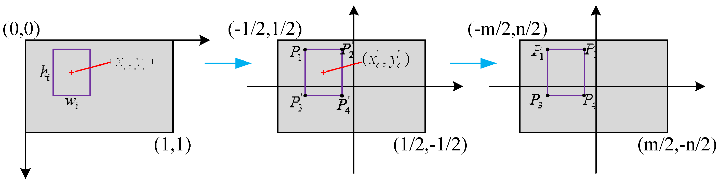
The loss function of YOLO v4 has a satisfactory effect in the training process, but it also leads to new problems. Owing to the loss function, the prediction frame coordinates given by YOLO are normalized center point coordinates, and the width and height values that cannot be directly applied to the positioning algorithm. To achieve high-accuracy building target positioning, a single prediction box is used as an example to provide the prediction frame coordinate calculation method in the image coordinate frame.

The conversion process is shown in Figure 3. Considering the four corner points of the prediction frame as an example, the position of the prediction frame output by YOLO can be converted into the image coordinate system using the following method. First, the YOLO output information (width, height, and image center position) is converted into a normalized coordinate system with the image center as the origin.

$$\begin{gathered} x_c^{\prime }=x_i-1/2,y_c^{\prime }=1/2-y_i \\ {w}_i\prime =w_i,h_i^{\prime }=h_i \end{gathered}$$

(4)

Subsequently, the coordinates of the corner points of the predicted frame in this coordinate system are calculated.

$$\left[\begin{array}{c}{x}_1^{\prime }\\ x_2^{\prime }\\ x_3^{\prime }\\ x_4^{\prime }\end{array}\begin{array}{c}\\ \end{array}\begin{array}{c}{y}_1^{\prime }\\ y_2^{\prime }\\ y_3^{\prime }\\ y_4^{\prime }\end{array}\right]=\left[\begin{array}{c}{x}_c^{\prime }-w_i/2\\ x_c^{\prime }+w_i/2\\ x_c^{\prime }-w_i/2\\ x_c^{\prime }+w_i/2\end{array}\begin{array}{c}\\ \\ \end{array}\begin{array}{c}\\ \\ \end{array}\begin{array}{c}{y}_c^{\prime }+h_i/2\\ y_c^{\prime }+h_i/2\\ y_c^{\prime }-h_i/2\\ y_c^{\prime }-h_i/2\end{array}\right]$$

(5)

Finally, the coordinates are enlarged according to the original size of the image ($m\ast n$) to obtain the coordinates of the corner points, $P_s(x_s,y_s)$, in the image coordinate frame.

$$\left[\begin{array}{c}{x}_s\\ y_s\end{array}\right]=\left[\begin{array}{cc}m& 0\\ 0& n\end{array}\right]\times \left[\begin{array}{c}{x}_s^{\prime }\\ y_s^{\prime }\end{array}\right]$$

(6)

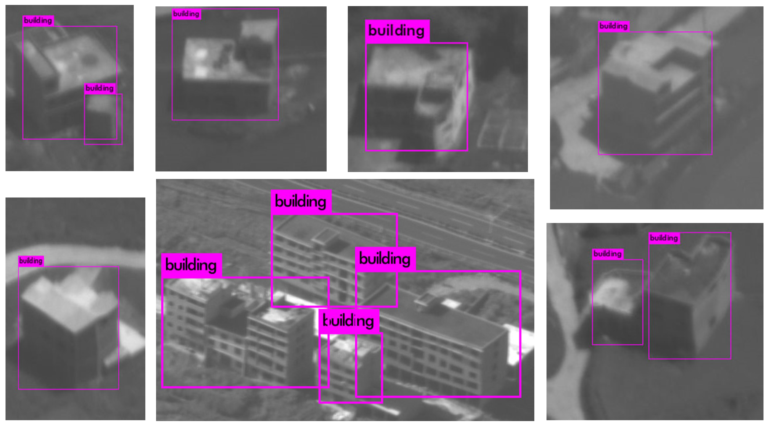
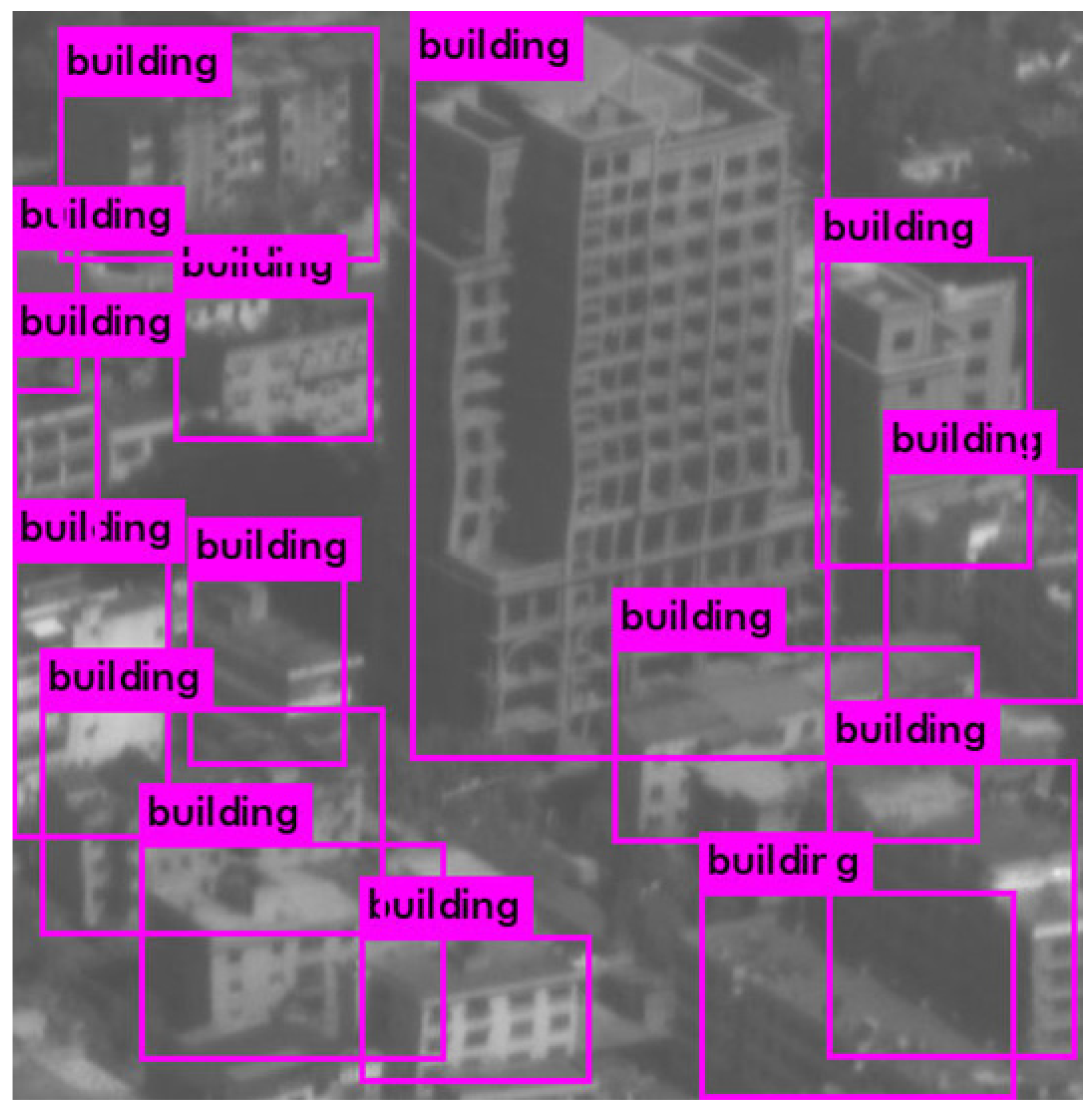
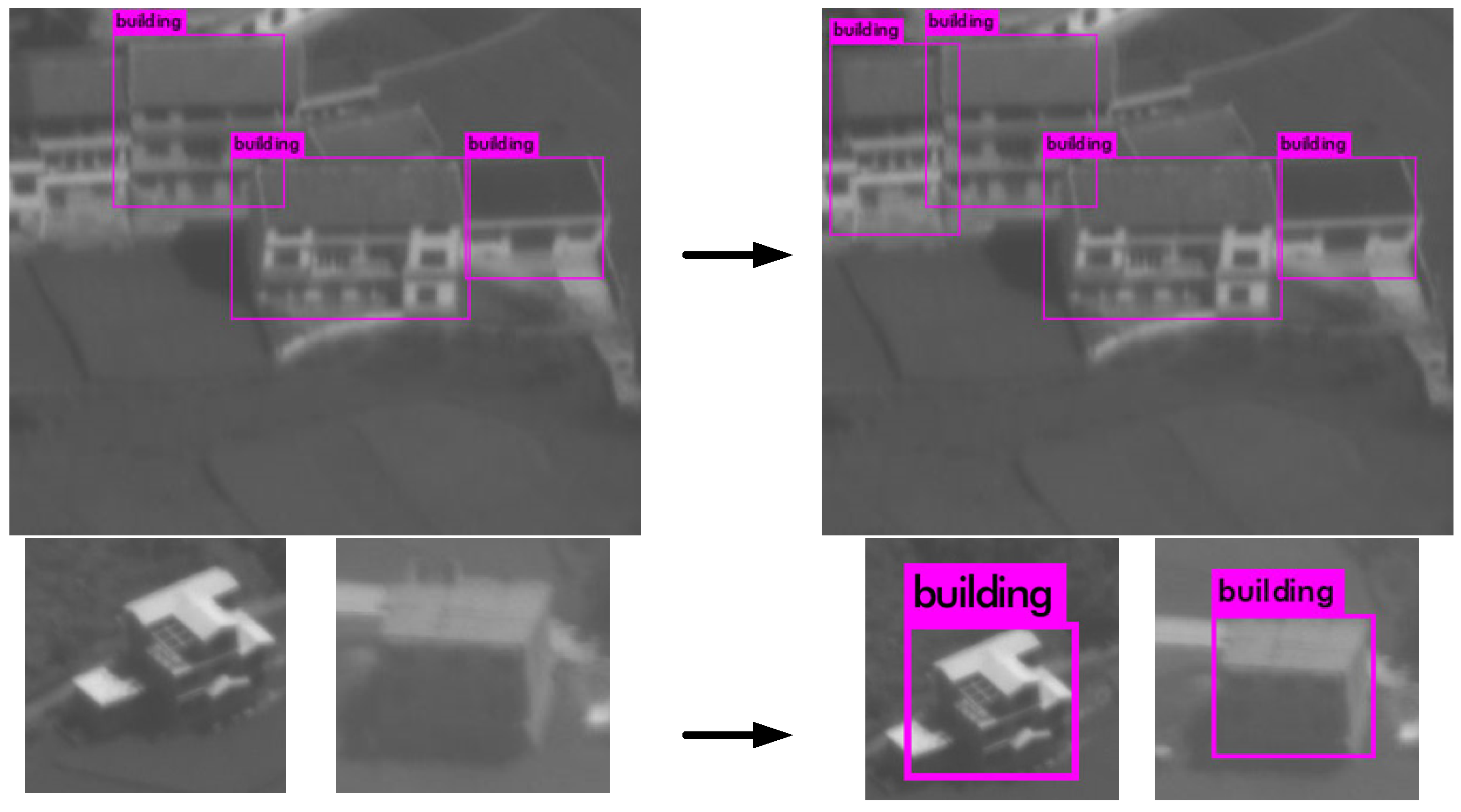
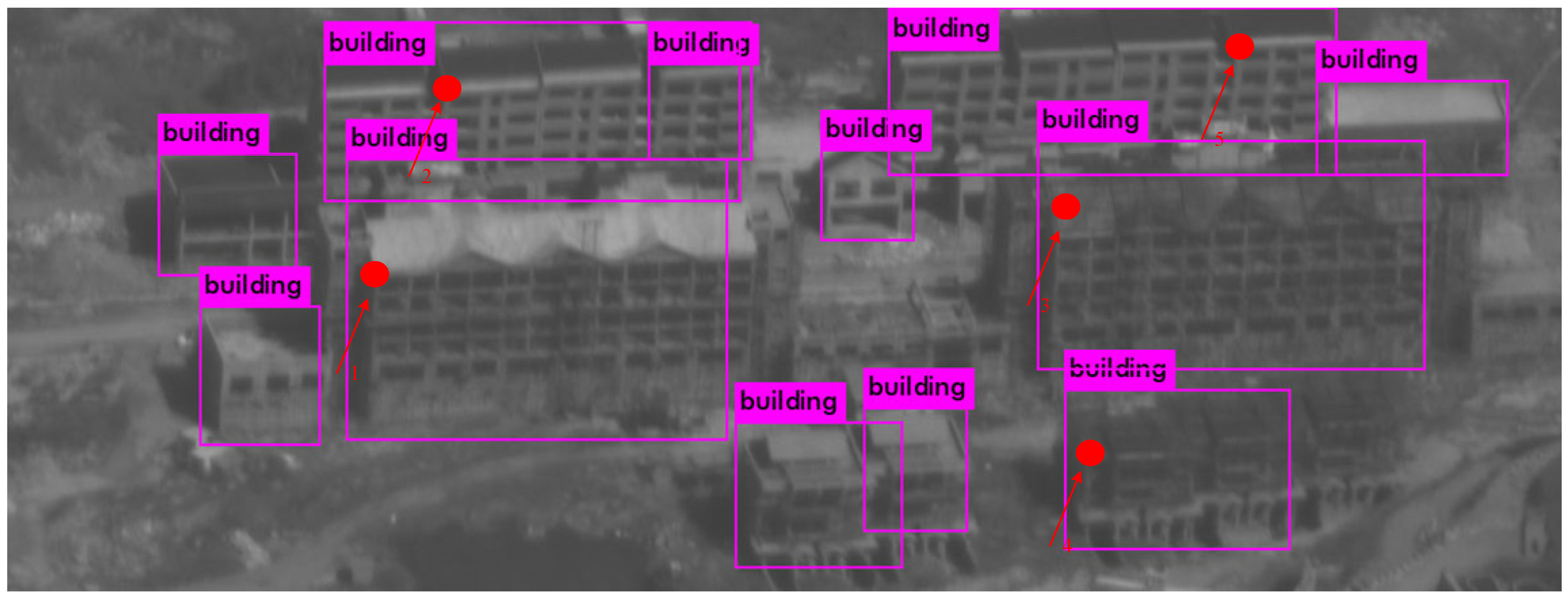
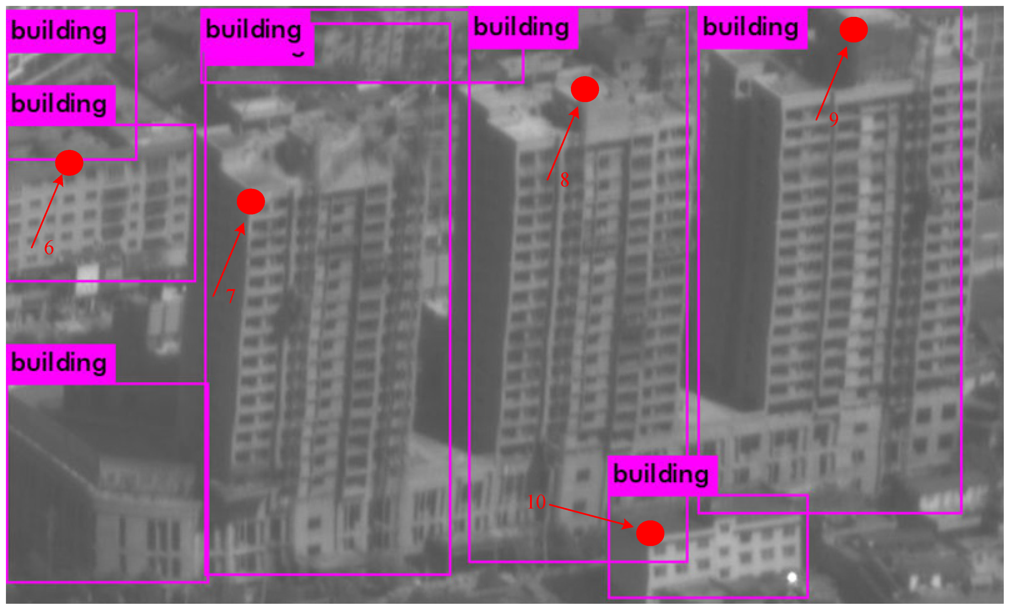
Additionally, this study improves the training speed of the detection algorithm by adjusting the initial value and decline of the learning rate. To facilitate the subsequent target positioning process, the detection algorithm can output the pixel coordinates of the prediction box in the image coordinate frame to be output in real time. Figure 4 and Figure 5 show the detection effect of the partial verification set, illustrating the detection results for small scattered buildings and dense urban buildings, respectively. The optimized building detection algorithm can better identify blocked buildings and small buildings in large-scale images. A comparison with the original YOLO v4 is shown in Figure 6.

3. Building Target Geo-Location Algorithm

The building target location algorithm aims to obtain accurate geo-location of the target point. The aerial cameras may produce inverted images because of the structure of the camera’s optical system and the scanning direction. However, the image is rotated in post-processing, so the image results still present a positive image. It is found that the top and bottom of the building usually have the same latitude and longitude $(\lambda ,\phi )$, but they differ in the height (h). Considering that no elevation error exists in the positioning result of the bottom of the building calculated by the collinear equation, the precise latitude and longitude information of the bottom of a building can be used as the overall building latitude and longitude. Furthermore, the height of targets on the building can be calculated by the algorithm provided in this section to improve the positioning accuracy of the building target.

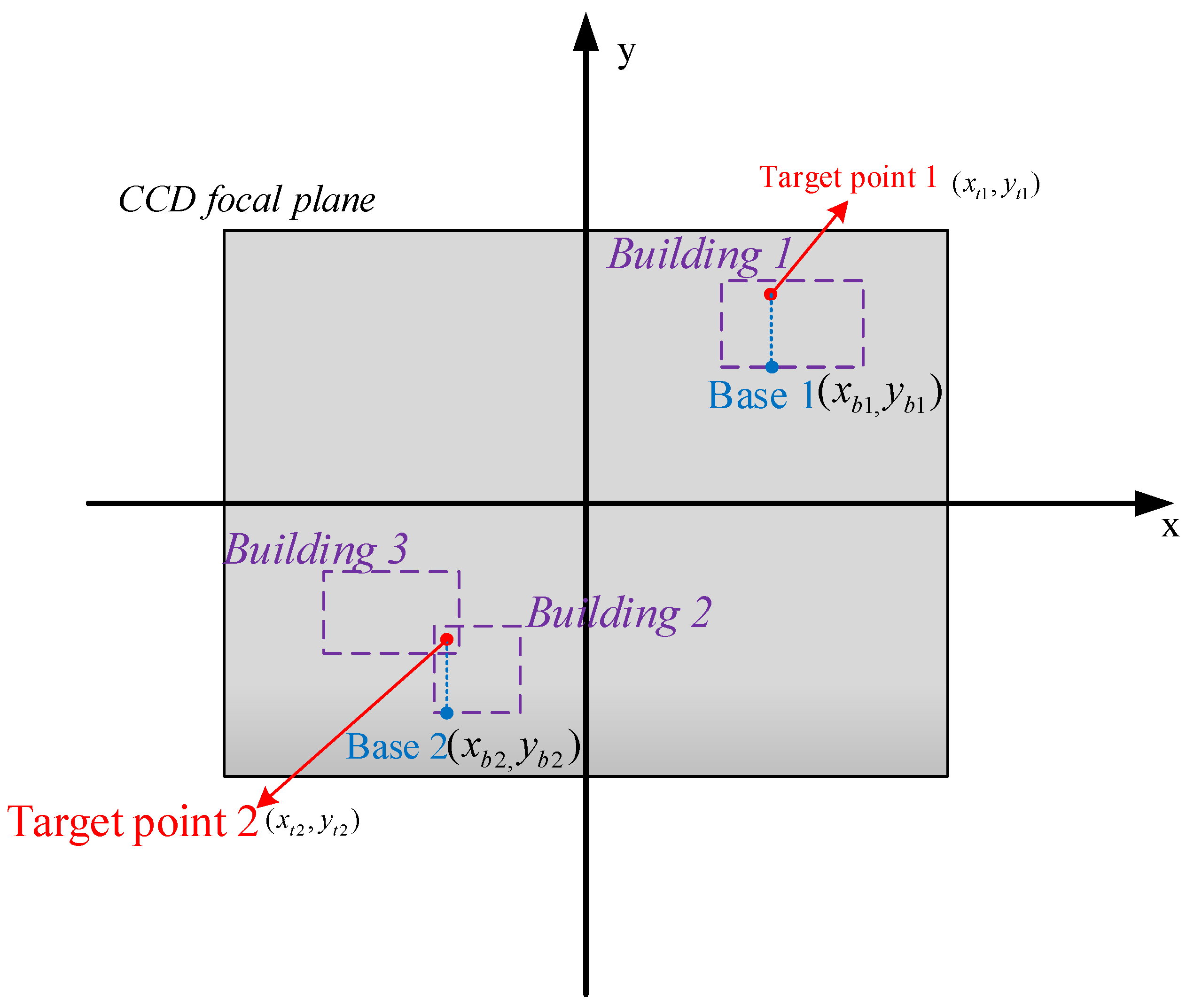
The building detection algorithm described in Section 2 can automatically detect buildings in remote sensing images and provide the position of the building prediction box in the image coordinate frame. The high-accuracy geo-location of building targets can be obtained in two steps. First, the target points on the same y-axis in the prediction box are considered having the same latitude and longitude. Subsequently, the appropriate base point position is selected and is regarded as the standard latitude and longitude of the target on a certain Y-axis. Second, the elevation information of the target point in the prediction frame is calculated according to the proposed building height algorithm. The base point is proposed to determine the latitude and longitude of the target point on a building. The base point is determined by the prediction box provided by the building detection algorithm. Considering that the aerial remote sensing image appears positive, the bottom of the prediction box (with the smaller y coordinate value) is usually selected as the base point. It should be noted that the buildings in the remote sensing image may overlap, so the prediction boxes in the image will also overlap. This phenomenon occurs because the building in front (i.e., closer to the airborne camera) blocks the building at the back. Hence, only the prediction frame of the building in front should be considered and is reflected in the image coordinate frame as a prediction box with a small Y-axis coordinate. As shown in Figure 7, the latitude and longitude of target points 1 and 2 are calculated by the base points 1 and 2, respectively.

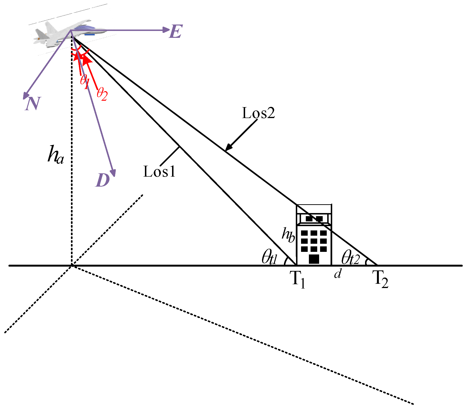
According to the difference between the image acquisition methods of line array and area array aerial cameras, the target point on the top floor of the building is used as an example. Two building height algorithms are presented in this paper. The line array camera can provide angle information when each line of the image is scanned, implying that the top and bottom of the building have different imaging angles. The geometric relationship when the linear array aerial camera obtains the building image is shown in Figure 8.

In this figure, $T_1$ and $T_2$ are the location results of the bottom and top of the building, which are calculated using the geo-location algorithm; ${\theta }_1$ and ${\theta }_2$ are the corresponding imaging angles; $h_b$ is the height of the building; d is the distance between $T_1$ and $T_2$; and $h_a$ is the altitude of the aircraft. The height of the building can be calculated by trigonometric functions, as shown in Equations (7) and (8).

$${\theta }_{t2}=\pi /2-{\theta }_2$$

(7)

$$h_b=d\times \tan {\theta }_{t2}$$

(8)

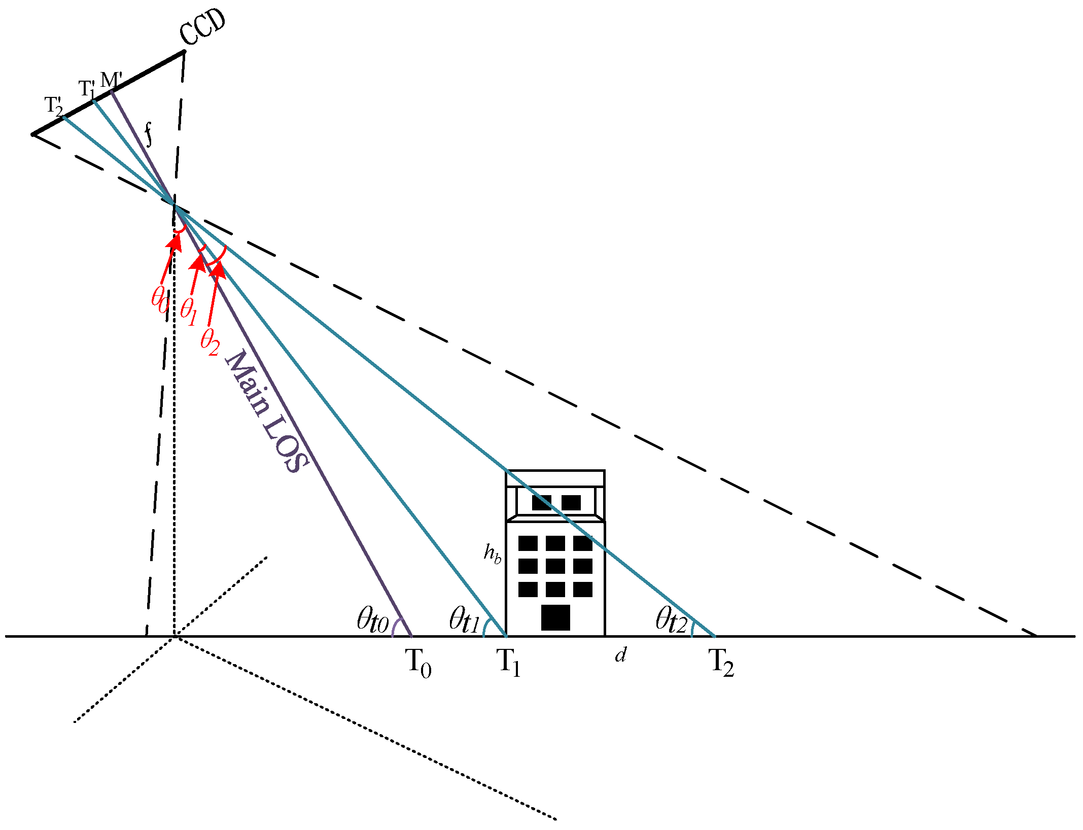
If the remote sensing image is acquired by an area array camera, the calculation process is more complicated. The area array camera records the imaging angle ${\theta }_0$ of the main optical axis (also called line of sight, LOS) of the camera when obtaining each image. The angles corresponding to the top and bottom of the building in the image should be calculated through the geometric relationship, as shown in Figure 9.

In this figure, $T_1^{\prime }(m_1,n_1),T_2{}^{\prime }(m_2,n_2)$ are the projection positions of the top and bottom of the building on the CCD, respectively. The number of pixels is represented by m and n. The angle ${\theta }_1$ between the imaging light at the bottom of the building and the main optical axis can be calculated using Equation (9), where f is the focal length of the camera and a is the size of a single pixel.

$${\theta }_1=\arctan (n_1\times a/f)$$

(9)

The angle ${\theta }_2$ between the imaging light at the bottom of the building and the main optical axis can be calculated similarly.

$${\theta }_2=\arctan (n_2\times a/f)$$

(10)

The angle parameters required by the building height algorithm can be calculated through geometric relationships as follows:

$${\theta }_{t0}=\pi /2-{\theta }_0,{\theta }_{t1}={\theta }_{t0}-{\theta }_1.$$

(11)

$${\theta }_{t2}={\theta }_{t1}-({\theta }_2-{\theta }_1).$$

(12)

The angle information required by the algorithm can be obtained using Equations (9)–(12), and the height of the building in the area array camera image can also be calculated using Equation (8).

As shown this algorithm, the height of building targets is calculated based on the geographic location of the bottom of the building combined with the direct positioning result of the target point. This article provides a simple and fast positioning algorithm based on the collinear equation as a reference. The geographic coordinates of a point in the remote sensing image can be calculated using a series of coordinate transformation matrices. $C_A^B$ represents the transformation process from the A coordinate frame to that of B; $C_A^B$ can be abbreviated as a block form; L is a third-order rotation matrix composed of cosines in the three-axis direction; and R is a translation column matrix composed of the origin position of the coordinate system. The inverse matrix of $C_A^B$ represents the transformation process from the B coordinate frame to that of A.

$$C_A^B=\left[\begin{array}{cccc}{l}_1& l_2& l_3& r_1\\ m_1& m_2& m_3& r_2\\ n_1& n_2& n_3& r_3\\ 0& 0& 0& 1\end{array}\right],C_A^B=\left[\begin{array}{cc}L& R\\ 0& 1\end{array}\right],C_B^A={(C_A^B)}^{-1}$$

(13)

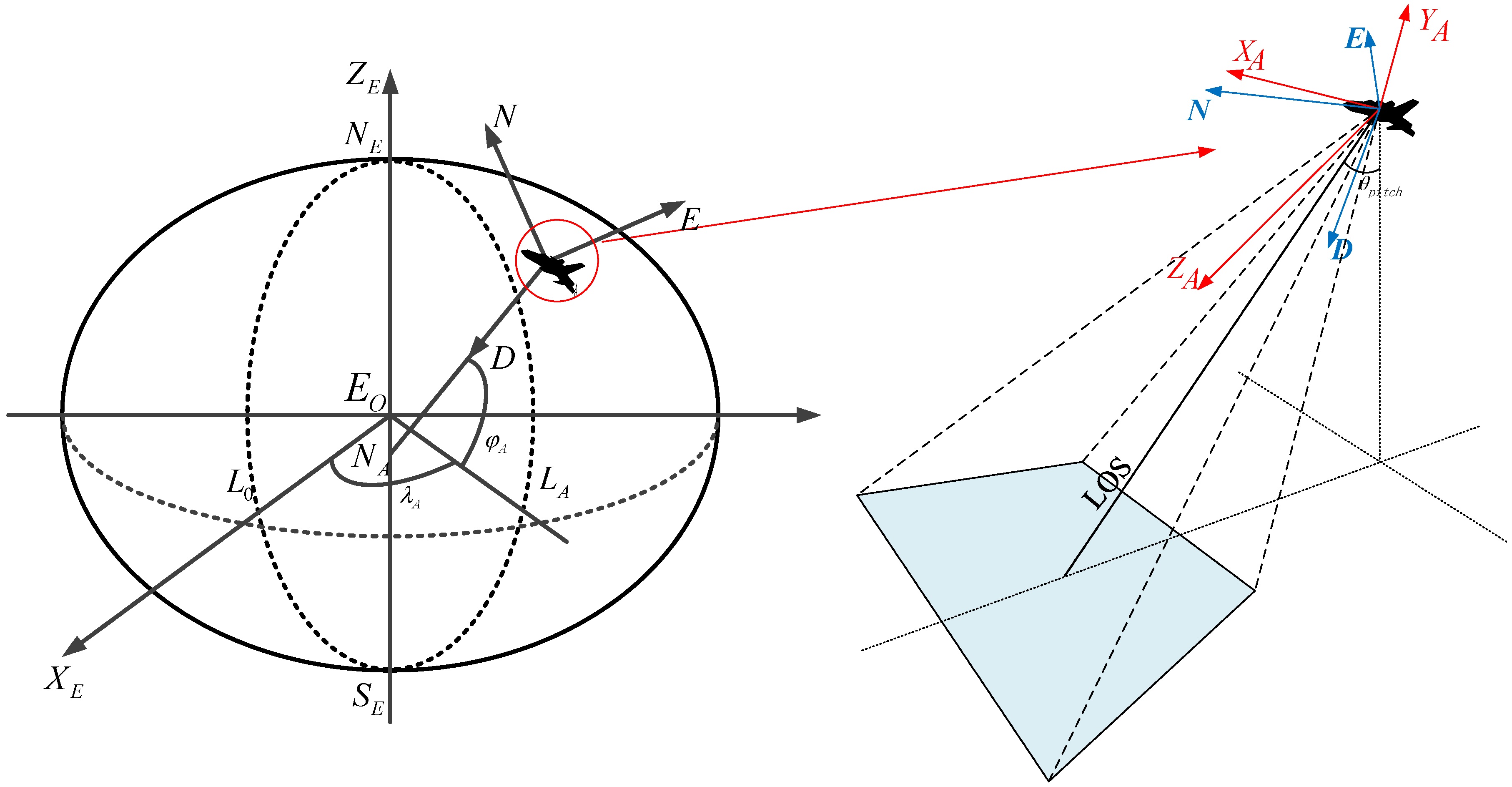
The earth-centered earth-fixed (ECEF) coordinate frame, also known as the earth coordinate frame, can be used to describe the position of a point relative to the earth’s center. The coordinates of the target projection point must be converted to the ECEF coordinate frame to establish the collinear equation in the earth coordinate frame. This process usually requires three coordinate frames: geographic coordinate frame, aircraft coordinate frame, and camera coordinate frame. Figure 10 is a schematic diagram of the corresponding coordinate frames.

The optical system is fixed on a two-axis gimbal, which is rigidly connected to the UAV or other airborne platforms. The camera coordinate frame (C) and aircraft coordinate system (A) can be established with the center of the optical system as the origin. The X-axis of the aircraft frame points to the nose of the aircraft, the Y-axis points to the right wing, and the Z axis points downward to form an orthogonal right-handed set. The attitude of the camera can be described by the inner and outer frame angles, ${\theta }_{pitch}$ and ${\theta }_{roll}$, respectively, and the transformation matrix of the camera frame and aircraft frame is as expressed in Equation (14).

$$C_A^C=\left[\begin{array}{cccc}\cos {\theta }_{pitch}& 0& -\sin {\theta }_{pitch}& 0\\ 0& 1& 0& 0\\ \sin {\theta }_{pitch}& 0& \cos {\theta }_{pitch}& 0\\ 0& 0& 0& 1\end{array}\right]\times \left[\begin{array}{cccc}1& 0& 0& 0\\ 0& \cos {\theta }_{roll}& \sin {\theta }_{roll}& 0\\ 0& -\sin {\theta }_{roll}& \cos {\theta }_{roll}& 0\\ 0& 0& 0& 1\end{array}\right]$$

(14)

As shown in Figure 8, according to the established method, the geographic coordinate frame is also called the north-east-down (NED) coordinate frame and is used to describe the position and attitude of the aircraft. The position of the airborne camera is considered as the origin, the N and E axes point to the real north and real east, and the D axis points to the geocentric along the normal line of the earth ellipsoid. Equation (15) is the transformation matrix between the A and NED coordinate frames, where attitude angles φ, θ, and ψ represent roll, pitch, and yaw angles, respectively.

$$C_{NED}^A=\left[\begin{array}{cccc}1& 0& 0& 0\\ 0& \cos \phi & \sin \phi & 0\\ 0& -\sin \phi & -\cos \phi & 0\\ 0& 0& 0& 1\end{array}\right]\times \left[\begin{array}{cccc}\cos \theta & 0& -\sin \theta & 0\\ 0& 1& 0& 0\\ \sin \theta & 0& \cos \theta & 0\\ 0& 0& 0& 1\end{array}\right]\times \left[\begin{array}{cccc}\cos \psi & \sin \psi & 0& 0\\ -\sin \psi & \cos \psi & 0& 0\\ 0& 0& 1& 0\\ 0& 0& 0& 1\end{array}\right]$$

(15)

The ECEF coordinate system can describe the position of the target, and its coordinate value can be converted into the geo-location information (i.e., latitude, longitude, and altitude). The origin of the ECEF coordinate frame is at the geometric center of the earth, where the X-axis points to the intersection of the equator and prime meridian, the Z-axis points to the geographic north pole, and the Y-axis forms an orthogonal right-handed set. Equation (16) is the conversion formula between the ECEF coordinate values and geo-location information. Equation (17) is the transformation matrix between the ECEF coordinate frame and NED coordinate frame, where λ, ϕ, and h correspond to longitude, latitude, and altitude, respectively.

$$\left[\begin{array}{c}{X}_E\\ Y_E\\ Z_E\end{array}\right]=\left[\begin{array}{c}(R_n+h)\cos \phi \cos \lambda \\ (R_n+h)\cos \phi \sin \lambda \\ (R_n(1-e^2)+h)\sin \phi \end{array}\right]$$

(16)

$$C_{ECEF}^{NED}=\left[\begin{array}{cccc}1& 0& 0& 0\\ 0& 1& 0& 0\\ 0& 0& 1& R_n+h\\ 0& 0& 0& 1\end{array}\right]\times \left[\begin{array}{cccc}-\sin \phi & 0& \cos \phi & 0\\ 0& 1& 0& 0\\ -\cos \phi & 0& -\sin \phi & 0\\ 0& 0& 0& 1\end{array}\right]\times \left[\begin{array}{cccc}\cos \lambda & \sin \lambda & 0& 0\\ -\sin \lambda & \cos \lambda & 0& 0\\ 0& 0& 1& 0\\ 0& 0& 0& 1\end{array}\right]\times \left[\begin{array}{cccc}1& 0& 0& 0\\ 0& 1& 0& 0\\ 0& 0& 1& R_n{e}^2\sin \phi \\ 0& 0& 0& 1\end{array}\right]$$

(17)

If $T_C^{\prime }$ is the position of the target projection point in the camera coordinate system, then its coordinates in the earth coordinate system $T_E^{\prime }$ can be calculated using the above transformation matrices.

$$T_E{}^{\prime }=\left[\begin{array}{c}{x}_T{}^{\prime }\\ y_T{}^{\prime }\\ z_T{}^{\prime }\\ 1\end{array}\right]=C_{NED}^{ECEF}\times C_A^{NED}\times C_C^A\times T_C{}^{\prime }$$

(18)

The collinear equation in the ECEF coordinate frame is composed of $T_E^{\prime }$ and the origin $O_C$ of the camera coordinate frame.

$$L:\frac{x_T-x_C}{x_T^{\prime }-x_C}=\frac{y_T-y_C}{y_T^{\prime }-y_C}=\frac{z_T-z_C}{z_T^{\prime }-z_C},O_C=[X_C,Y_C,Z_C]$$

(19)

The position of the target in the ECEF coordinate system can be obtained by solving the intersection of the collinear equation and earth model. The earth model uses the ellipsoid model or DEM data. Our study uses the ellipsoid model as an example. If the altitude of the target is $h_T$, the earth ellipsoid equation of the target can be expressed as Equation (20) [6].

$$\frac{x_T{}^2}{{(R_e+h_T)}^2}+\frac{y_T{}^2}{{(R_e+h_T)}^2}+\frac{z_T{}^2}{(R_e+h_T)\times {(1-e^2)}^{1/2}}=1,$$

(20)

where $R_e=\mathrm{6,378,137}\mathrm{m}$ and $R_p=\mathrm{6,356,752}\mathrm{m}$ are the semi major and semi-minor axes, respectively.

The geo-location information of the target can be obtained through an iterative algorithm based on the calculation results of Equations (19) and (20).

$$\begin{gathered} \{\begin{array}{l}{N}_0=R_e\\ h_0={[{(x_T)}^2+{(y_T)}^2+{(z_T)}^2]}^{1/2}-{(R_e{R}_p)}^{1/2}\\ {\phi }_0=\arctan \left\{\frac{z_T[(1-e^2)N_0+h_0]}{{[{(x_T^{})}^2+{(y_T)}^2]}^{1/2}(N_0+h_0)}\right\}\end{array} \\ \{\begin{array}{l}{N}_i=\frac{R_E}{{(1-e^2{\sin }^2{\phi }_{i-1})}^{1/2}}\\ h_i=\frac{{[{(x_T)}^2+{(y_T)}^2]}^{1/2}}{\cos {\phi }_{i-1}}-N_{i-1}\\ {\phi }_i=\arctan \left\{\frac{z_T[(1-e^2)N_{i-1}+h_{i-1}]}{{[{(x_T)}^2+{(y_T)}^2]}^{1/2}(N_{i-1}+h_{i-1})}\right\}\end{array} \end{gathered}$$

(21)

$${\lambda }_0=\arctan (\frac{y_T}{x_T}),\lambda =\{\begin{array}{ccc}{\lambda }_0& \hspace{1em}\hspace{1em}& x_T>0\\ {\lambda }_0+\pi & \hspace{1em}\hspace{1em}& x_T<0, {\lambda }_0<0\\ {\lambda }_0-\pi & \hspace{1em}\hspace{1em}& x_T<0, {\lambda }_0>0\end{array}$$

(22)

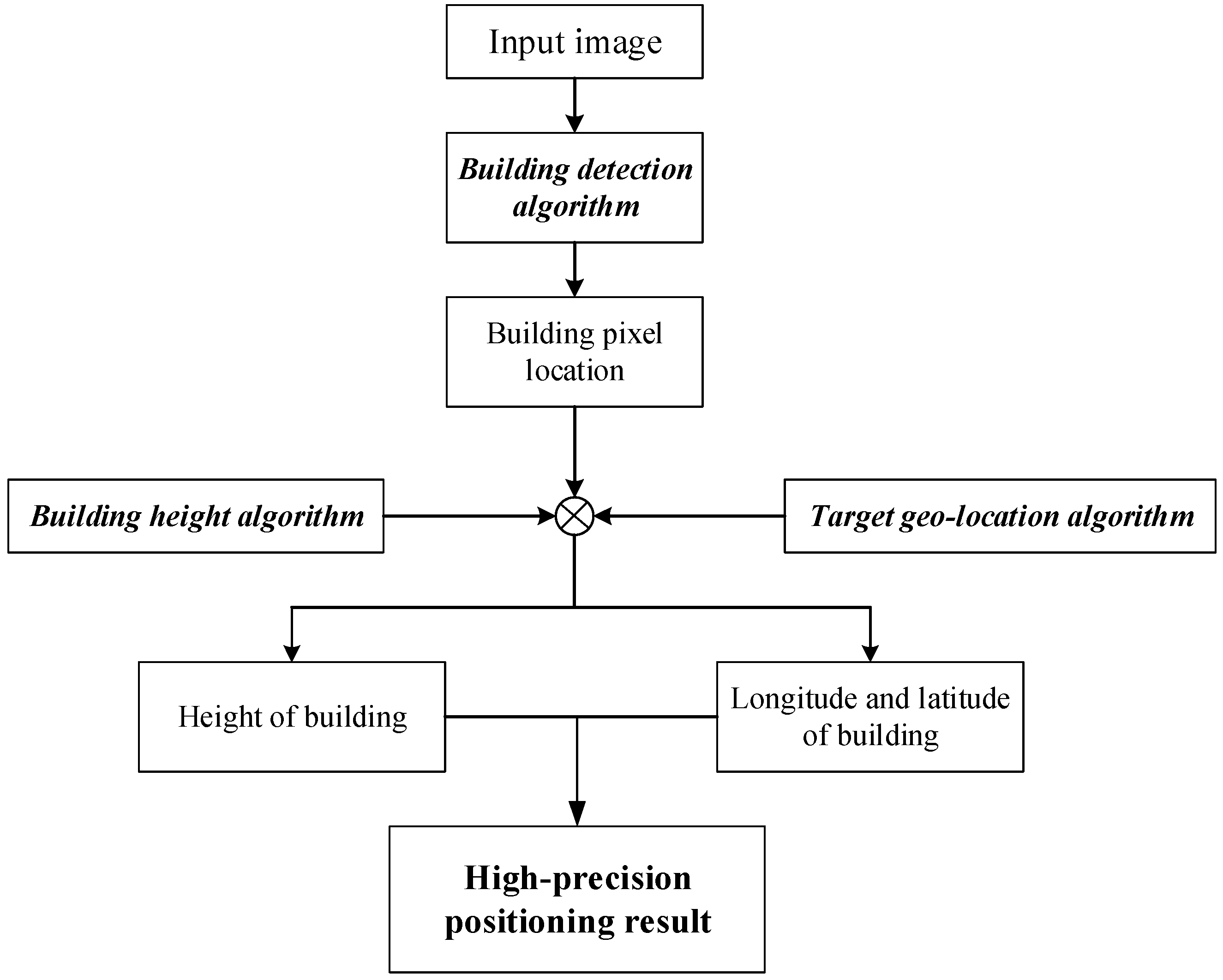
The precise geo-location information of the building $({\lambda }_B,{\phi }_B,h_T)$ can be obtained using the above algorithm. Meanwhile, the precise geographic information of a target on the building consists of two parts: the latitude and longitude of the bottom of the building $({\lambda }_B,{\phi }_B)$ and the height of the target point $(h_T)$. The complete positioning process is illustrated in Figure 11.

4. Experimental Results

4.1. Simulation Results

The traditional positioning algorithm is used to locate the target on the building in the simulation environment. Through a simulation analysis of the positioning error caused by the height of the building target, the importance of the building target positioning algorithm is verified. The error between the true position of the target ($T_E^R=\left[\begin{array}{ccc}{x}_r& y_r& z_r\end{array}\right]$) and the positioning result ($T_E^D=\left[\begin{array}{ccc}{x}_d& y_d& z_d\end{array}\right]$) can be calculated using the spatial two-point distance formula, as shown in Equation (23).

$$d=\sqrt{{(x_r-x_d)}^2+{(y_r-y_d)}^2+{(z_r-z_d)}^2}$$

(23)

$$\Delta y=f(x+\Delta x_1,x_2+\Delta x_2,\mathrm{...},x_n+\Delta x_n)-f(x_1,x_2,\mathrm{...},x_n)$$

(24)

The spatial distance formula is only suitable for calculating a single positioning error. To simulate the positioning algorithm, a suitable random number should be selected to replace the random error in the actual positioning process. In this study, an error model is established based on the Monte Carlo method, as shown in Equation (24). In the equation, $\Delta y$ is the positioning error, and the result of $\Delta y$ is equivalent to the error value calculated by the spatial distance formula in a single simulation. The measured value of each parameter required by the geo-location algorithm is $x_1,x_2,\mathrm{...},x_n$, and $\Delta x_n$ is the increment according to the standard normal distribution, which represents random errors caused by sensor measurements. The parameters used in the simulation process are presented in

Table 1. Simulation experiment parameters.

Data	Unit	Real Value	Error Value
Camera Latitude	${\mathsf{\phi }}_{\mathrm{A}}/(°$)	35	0.0001
Camera Longitude	${\mathsf{\lambda }}_{\mathrm{A}}/(°)$	110	0.0001
Camera Altitude	${\mathrm{h}}_{\mathrm{A}}/\mathrm{m}$	10,000	10
Camera Attitude(Yaw)	$\psi /(°)$	0	0.06
Camera Attitude(Pitch)	$\theta /(°)$	3	0.02
Camera Attitude(Roll)	$\mathsf{\phi }/(°)$	0	0.02
Gimbal Angel(Outer)	${\theta }_{roll}/(°)$	40–80	0.006
Gimbal Angel(Inner)	${\theta }_{pitch}/(°)$	−1.5	0.006
Pixel Number	N/A	3000*4000	N/A
Focal Length	f/(m)	1.5	N/A
Pixel Size	a/(nm)	8	N/A

.

According to the positioning error values obtained by the simulation analysis, various evaluation criteria can be used for the positioning accuracy, such as the average positioning error, positioning standard deviation, and circle probability error. The average positioning error refers to the average of all positioning errors in a simulation experiment. The positioning standard deviation refers to the standard deviation of the sequence consisting of multiple positioning error data, calculated using the standard deviation formula. The circular error probability (CEP) refers to the radius of a circle containing half of the positioning results centered on the true position of the target in multiple simulations. The lower the value of the three evaluation criteria, the higher is the accuracy of the positioning algorithm.

Figure 12 shows a comparison of the calculation results of the three error evaluation criteria when the simulation positioning target is located on a building with the height of 70 m. The specific simulation parameters are presented in Table 1. The horizontal axis of the image is the change in the imaging angle, and the vertical axis is the error value. The figure shows that, as the imaging angle increases, the three error types exponentially increase. The larger the imaging inclination, the greater is the positioning error caused by the height of the building. When the imaging angle is 75°, the average positioning error is close to 150 m. Additionally, although the overall change of CEP shows an increasing trend, CEP does not increase regularly with the increase in the imaging angle. This is caused by the calculation principle of CEP. The building target positioning errors include large height errors, and CEP ignores such errors. CEP is usually aimed at 2D plane errors and treats all positioning results as the same plane; thus, CEP is not suitable for error analysis of targets on buildings. Therefore, the analysis of positioning error in this study mainly uses the average positioning error.

Figure 13 shows a schematic diagram of the error change of the building target height ranging from 10 m to 100 m. The horizontal and vertical axes represent the target height of the building and average positioning error, respectively. The positioning results in the figure are also obtained in the simulation environment using the traditional target positioning algorithm. Evidently, the target height and imaging angle are directly related to the positioning error. When using traditional algorithms to locate the target on a building, even if the height of the building is only 10 m, a total positioning error of 63 m will occur when the imaging angle is 65°. Under the same imaging conditions, if the target point is on the ground, the positioning error is approximately 47 m. The positioning accuracy of traditional algorithms has decreased by nearly 33%. When the inclination angle reaches 70°, the error value increases by nearly 90 m, and the positioning error is as high as 126 m when the target height is 80 m.

Figure 14 shows a schematic diagram of the distribution of positioning results in 10,000 simulation experiments. The experimental parameters were a building with the height of 70 m and an imaging angle of 60°. The remaining parameters are listed in Table 1. Clearly, when the target has a building elevation error, the positioning results of the traditional positioning algorithm are comprehensively affected. In addition to the extreme height error, the positioning accuracy of the target point’s latitude and longitude also decreases. When a traditional geo-location algorithm is used to position the ground target, the average positioning error of the latitude is $2.8738\times {10}^{-6}°$, and the that of the longitude is $2.3203\times {10}^{-6}°$. When the target is on the top floor of the building, the average latitude error of the positioning result increases to $9.0545\times {10}^{-4}°$, and the average longitude error increases to $1.5867\times {10}^{-4}°$.

From the simulation analysis results in this section, we can conclude that the traditional positioning algorithm applied directly to the target on the building causes a great positioning error. Therefore, the positioning algorithm and positioning ability of building targets should be enhanced.

4.2. Actual Remote-Sensing Image Test Results

In this section, the actual working effect of the established building target geo-location algorithm is tested. The test data include the oblique aerial remote sensing image captured by the airborne camera. The building target geo-location algorithm and traditional positioning algorithm proposed in this study are used to locate the target simultaneously. The effectiveness of the building target positioning algorithm was verified by comparing the positioning results of the two algorithms. The standard latitude and longitude information of the target is measured by a single-station handheld differential global position system (DGPS), and the precise elevation information of the building is measured by an electronic total station. The accuracy of the DGPS used in the experiment is within 0.5 m, which is sufficient to meet the requirements as a standard reference value. To prove the wide applicability of the algorithm, two experimental pictures were obtained from two different aerial photographs. In the figure, the top layer of some buildings was randomly selected as the target point, and the positioning results of the different algorithms were compared. During the positioning process, the building detection algorithm was used to detect the remote sensing image. The results are shown in Figure 15 and Figure 16. Figure 15 mainly includes shorter buildings (<10 floors), and Figure 16 includes taller buildings (>10 floors). The parameters of the aircraft and camera during image acquisition are presented in

Table 2. Parameters of the camera and aircraft.

Camera Parameters	Figure 13	Figure 14
Camera Latitude/°	106.2981	106.3874
Camera Longitude/°	26.2294	26.2665
Camera Altitude/m	16582	17654
Aircraft Yaw/°	0.3901	0.3906
Aircraft Pitch/°	0.02	0.0207
Aircraft Roll/°	−0.0001	0.000427
Gimbal Roll/°	70.024	69.7302
Gimbal Pitch/°	−2	−2
Altitude of Target Area/m	1410	1363

.

The building in Figure 15 is located in an urban community. The image was captured at 23.21° N–23.22° N and 105.85° E–105.87° E, and the height of buildings in the picture is between 10 and 25 m. The target points are randomly distributed on the top layer of the building, and the target is located using the traditional positioning algorithm and building target positioning algorithm, respectively.

Table 3. Positioning results of Figure 15.

Target Number	1	2	3	4	5
Target Latitude (R)/°	23.218790	29.219244	26.219365	26.219027	26.219778
Target Longitude (R)/°	105.865451	105.865336	105.866081	105.866182	105.866106
Target Altitude (R)/m	1432.7	1425.8	1433.7	1425.2	1427
Latitude of Positioning Results (T)/°	26.219077	26.219340	26.219558	26.218932	26.219849
Longitude of Positioning Results (T)/°	105.864553	105.864558	105.865464	105.865640	105.865491
Altitude of Positioning Results (T)/°	1410.02	1410.03	1410.01	1410.01	1410.02
Latitude of Positioning results (B)/°	26.218536	26.218935	26.219049	26.218656	26.219483
Longitude of Positioning Results (B)/°	105.864811	105.864791	105.865741	105.865909	105.865743
Altitude of Positioning Results (B)m	1431.56	1425.63	1433.53	1425.08	1426.68
Error of Traditional Algorithm (T)/m	97.7419	78.9521	84.4955	64.0555	67.876
Error of New Algorithm (B)/m	68.3784	62.932	47.86	44.29	45.263
Variation of Error/m	29.3635	16.0201	36.6355	19.7655	22.613
Accuracy Improvement (%)	0.3004	0.2029	0.4336	0.3086	0.3332

presents the specific positioning results of the experiment. In the table, R represents the real position of the target, and T and B represent the target position calculated by the traditional geo-location algorithm and building target geo-location algorithm, respectively. Experimental results show that the geo-location error of the target using traditional positioning algorithms is between 64.05 and 97.74 m. The building target positioning algorithm established in this study can reduce the positioning error to 44.29–68.37 m, and the positioning accuracy is significantly improved.

Figure 16 shows an aerial remote sensing image of some office buildings. In this image, most of the buildings have the height between 60 and 100 m (target numbers 7–9), while some are relatively short buildings (target numbers 6 and 10). The standard geo-location of the target is obtained through DGPS and the electronic total station. The specific positioning information and related errors are listed in

Table 4. Positioning results of Figure 16.

Target Number	1	2	3	4	5
Target Latitude (R)/°	26.248419°	26.248654°	26.249106°	26.249548°	26.249231°
Target Longitude (R)/°	105.956412°	105.956628°	105.956392°	105.956033°	105.956563°
Target Altitude (R)/m	1385.3	1425	1426.5	1428.2	1376.2
Error of Traditional Algorithm (T)/m	93.2859	109.7042	122.228	113.9909	85.3932
Error of New Algorithm (B)/m	61.6784	56.5252	68.7251	61.8253	61.1385
Variation of Error/m	31.6075	53.5042	53.5029	52.1656	24.2547
Accuracy Improvement (%)	0.3388	0.4847	0.4377	0.4576	0.284

. The positioning error of the traditional algorithm is between 85.39 and 122.23 m, and that of the building target positioning algorithm is between 61.13 and 68.72 m. Because of the higher target height, compared to that of the first experiment (Figure 13), the building target positioning algorithm improves the positioning accuracy more evidently. For higher buildings, the positioning accuracy can increase by 43%–48%.

5. Discussion

The above analysis is based on the overall error of the positioning result, which indicates the spatial distance between the positioning result and standard reference position of the target point. To clearly prove that the proposed algorithm can calculate the elevation information more effectively, the overall positioning error is decomposed into the horizontal position error (error of latitude and longitude) and height error. Moreover, the accuracy of the algorithm is evaluated separately, as presented in

Table 5. Results of decomposition error.

Target Number	1	2	3	4	5
Ground Error (T)/m	94.71	77.14	80.97	61.98	65.42
Altitude Error (T)/m	22.68	15.77	23.69	15.19	19.98
Ground Error (B)/m	68.37	62.93	47.86	44.29	45.26
Altitude Error (B)/m	1.14	0.17	0.17	0.12	0.32
Inherent Error/m	67.49	61.74	46.27	43.15	42.47
Target Number	6	7	8	9	10
Ground Error (T)/m	90.20	87.56	101.77	90.34	84.22
Altitude Error (T)/m	22.31	61.96	63.48	65.2	13.21
Ground Error (B)/m	61.67	56.49	68.74	61.79	61.13
Altitude Error (B)/m	0.07	2.03	1.48	1.80	0.44
Inherent Error/m	60.24	56.2	66.48	60.45	50.85

. In the table, the ground error is the latitude and longitude error between the position results and the standard reference value, which is a 2D distance error. The results show that the height error of the algorithm established in this study is within 2 m. However, the traditional algorithm regards the target in the image as being located on the same horizontal plane, and the height error is essentially equal to the height of the building. Compared to the traditional position algorithm, the algorithm proposed in this study also reduces the latitude and longitude positioning error of the building target. The algorithm’s ability to position the target’s latitude and longitude is related to the accuracy of the image parameter information. This is because the image parameters contain certain errors, such as those of carrier attitude angle and camera imaging angle. The positioning error caused by the image information is called the image inherent error in the table.

A comparison of the positioning results of the two algorithms is shown intuitively in Figure 17. Situations 1 and 2 in the figure are the positioning results of the target using traditional positioning algorithms and the proposed building target positioning algorithm, respectively. The order of the target points in the figure is arranged according to the actual height of the target (i.e., from low to high). As shown in the figure, regardless of whether the target is on a high-rise or low-rise building, the traditional positioning algorithm causes a large positioning error. Conversely, the proposed building target positioning algorithm improves the positioning accuracy by 20–48%. In summary, the algorithm proposed in this study can calculate the elevation of the building target effectively and can correct the latitude and longitude to a certain extent. This is widely applicable to various oblique aerial remote sensing images.

6. Conclusions

This study proposes a geo-location algorithm for targets in buildings. The algorithm uses deep learning to achieve automatic detection of building targets when acquiring images. Moreover, it provides a building height estimation model based on the location of the prediction box to achieve high-accuracy positioning of building targets. With the development of aeronautical photoelectric loads, oblique aerial remote sensing images are widely applied, and the requirements for image positioning capabilities are increasing. However, when the traditional positioning algorithm locates the building target in a single image, a large positioning error is generated. The positioning error of the building target has two main reasons. First, most of the existing long-distance positioning algorithms to locate the target are based on the collinear equation. The positioning result is the projection of the target on the ground rather than its real position. Second, the remote sensing image is essentially a 2D image that does not directly provide the height information of the target. Conversely, the algorithm proposed in this study remarkably improves the positioning accuracy of building targets and can be widely used in oblique aerial remote sensing images. The algorithm can also be used with various existing high-precision ground target positioning algorithms to improve its positioning effect on building targets. The limitation of the proposed method is that the detection algorithm can only output a rectangular prediction box, which may cause the prediction box to include other features apart from buildings. If the roof of a building is at a 45° angle, the prediction box can still completely cover the building. However, there must be a situation where the ground image is also covered in the prediction box. If a positioning target exists in the image at this time, it will inevitably lead to positioning errors during the automatic calculation by the algorithm. This problem can be solved by manually confirming the building target in the image. However, it should be noted that in real aerial remote sensing city images, no positioning target near the roof of the building usually exists. Owing to the large range of oblique imaging, the image of the near-roof building in an urban remote sensing image is usually other buildings in the distance. Compared to the entire image, the prediction box of low-rise buildings is small. The non-building area in the prediction box may only be 10 × 10 pixels and will not include ground positioning targets.

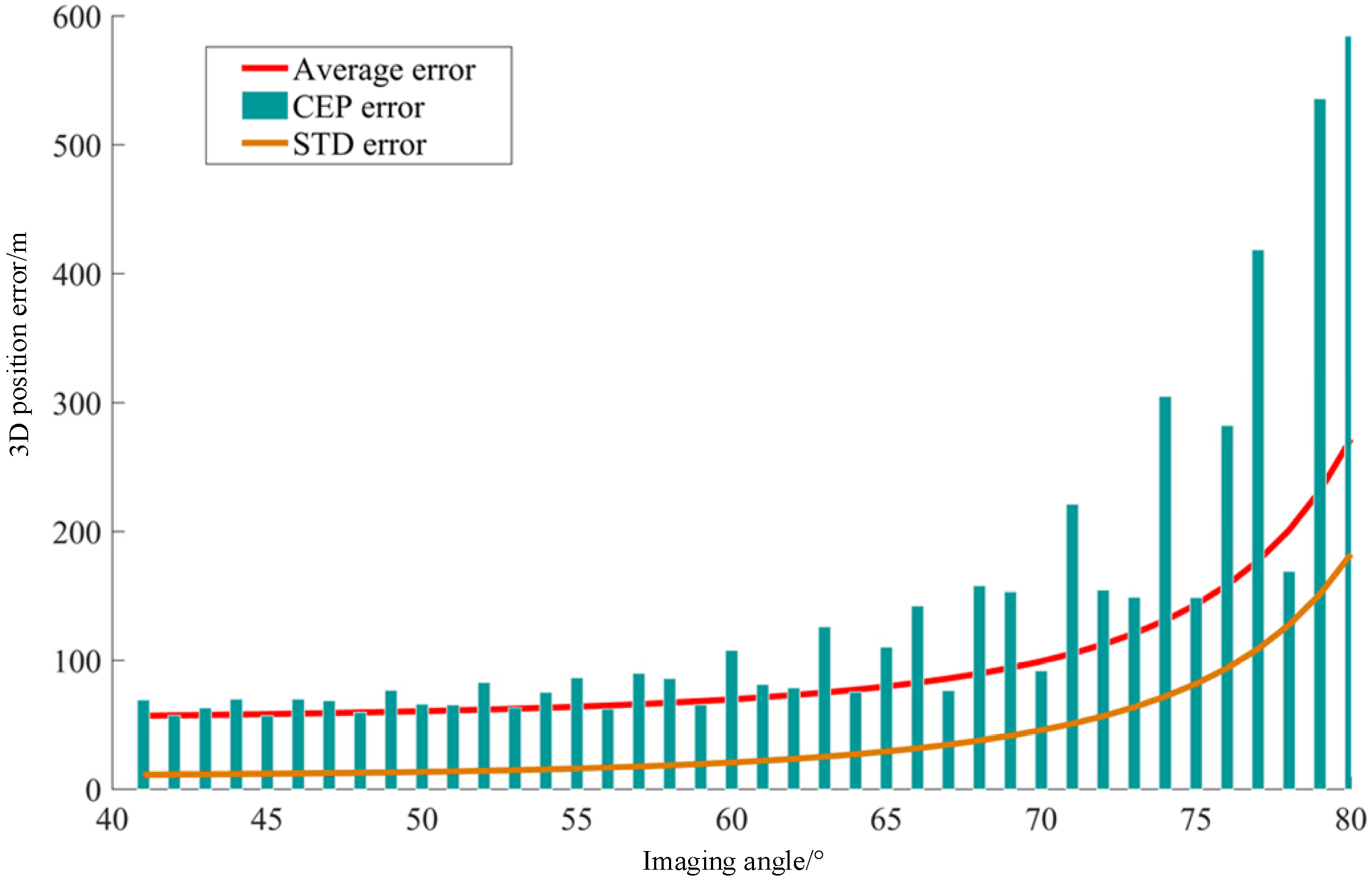
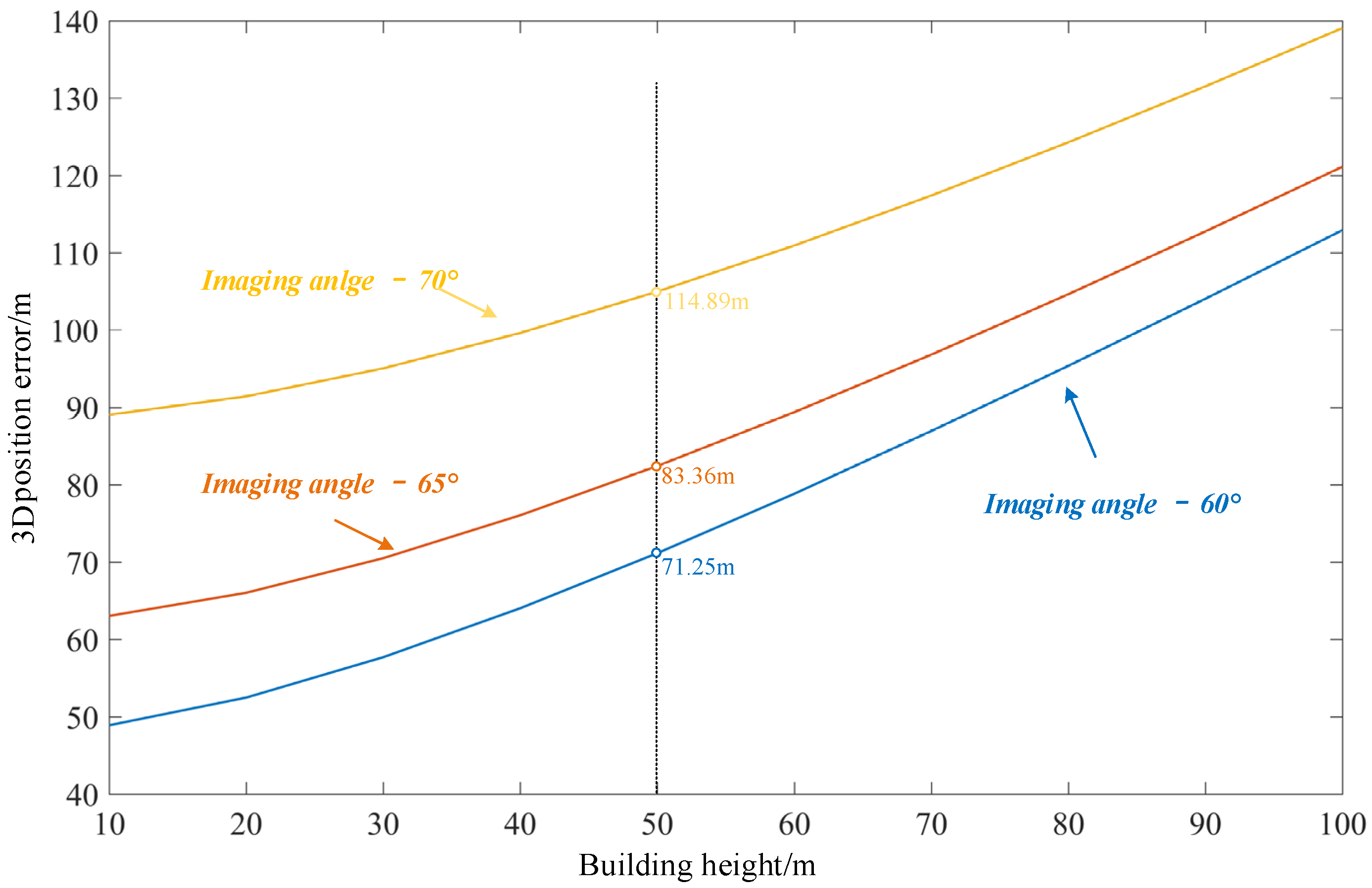
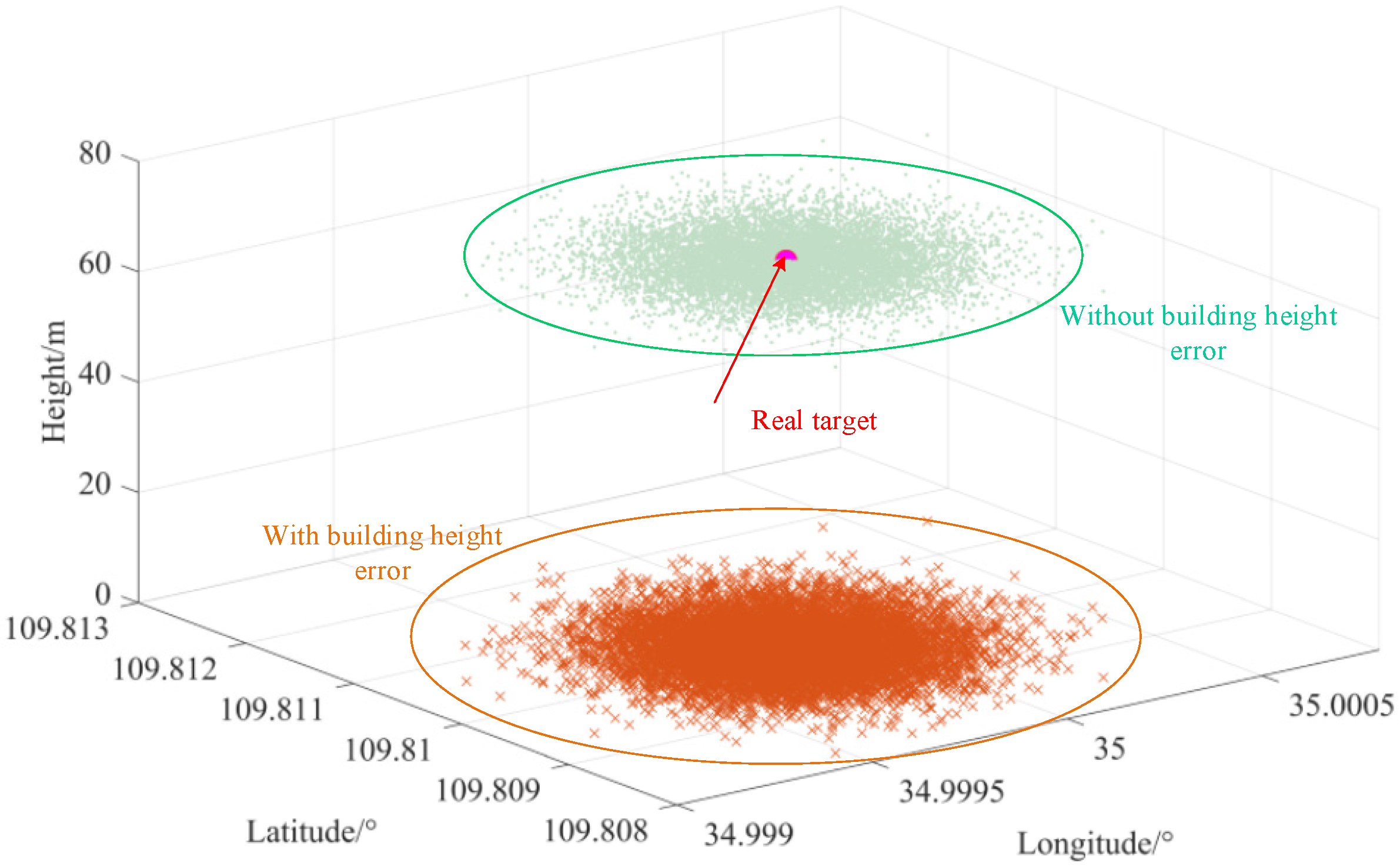
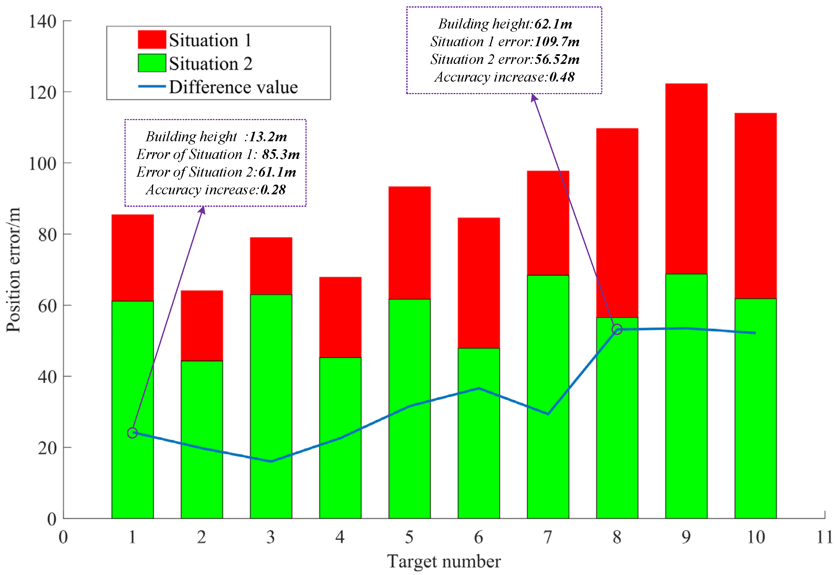
Experiments show that the proposed algorithm proposed can detect and estimate the height of buildings in an image. The algorithm can improve the accuracy by approximately 40% when the imaging angle is 70° and target height is 60 m. For buildings with a height of 20 m, the accuracy can be increased by approximately 25%. This algorithm can improve the accuracy of positioning, but the improvement effect is not fixed at 25–40%. This is because, in addition to the error caused by the target height, the positioning algorithm is also affected by other factors. For example, the positioning algorithm based on angle information will be affected by the accuracy of the angle measurement, and that based on laser distance measurement will be affected by the accuracy of the distance measurement. The higher the accuracy of the angle and distance measurements, the smaller is the error of the positioning algorithm and the greater is the relative weight of the influence of the building height error on the positioning result. Therefore, with the improvement of the accuracy of various angle and distance measuring sensors, the building target positioning algorithm established in this paper will be more effective for the optimization of traditional positioning algorithms and has greater practical significance.