Article

Deep Semantic Segmentation of Center Pivot Irrigation Systems from Remotely Sensed Data

by
Anesmar Olino de Albuquerque
1,
Osmar Abílio de Carvalho Júnior
1,*,
Osmar Luiz Ferreira de Carvalho
2,
Pablo Pozzobon de Bem
1,
Pedro Henrique Guimarães Ferreira
2,
Rebeca dos Santos de Moura
1,
Cristiano Rosa Silva
1,
Roberto Arnaldo Trancoso Gomes
1 and
Renato Fontes Guimarães
1
1
Departamento de Geografia, Campus Universitário Darcy Ribeiro, Asa Norte, Universidade de Brasília, DF, Brasília 70910-900, Brazil
2
Departamento de Engenharia Elétrica, Campus Universitário Darcy Ribeiro, Asa Norte, Universidade de Brasília, DF, Brasília 70910-900, Brazil
*
Author to whom correspondence should be addressed.
Remote Sens. 2020, 12(13), 2159; https://doi.org/10.3390/rs12132159
Submission received: 19 May 2020 / Revised: 29 June 2020 / Accepted: 1 July 2020 / Published: 6 July 2020

Abstract

:
The center pivot irrigation system (CPIS) is a modern irrigation technique widely used in precision agriculture due to its high efficiency in water consumption and low labor compared to traditional irrigation methods. The CPIS is a leader in mechanized irrigation in Brazil, with growth forecast for the coming years. Therefore, the mapping of center pivot areas is a strategic factor for the estimation of agricultural production, ensuring food security, water resources management, and environmental conservation. In this regard, digital processing of satellite images is the primary tool allowing regional and continuous monitoring with low costs and agility. However, the automatic detection of CPIS using remote sensing images remains a challenge, and much research has adopted visual interpretation. Although CPIS presents a consistent circular shape in the landscape, these areas can have a high internal variation with different plantations that vary over time, which is difficult with just the spectral behavior. Deep learning using convolutional neural networks (CNNs) is an emerging approach that provokes a revolution in image segmentation, surpassing traditional methods, and achieving higher accuracy and efficiency. This research aimed to evaluate the use of deep semantic segmentation of CPIS from CNN-based algorithms using Landsat-8 surface reflectance images (seven bands). The developed methodology can be subdivided into the following steps: (a) Definition of three study areas with a high concentration of CPIS in Central Brazil; (b) acquisition of Landsat-8 images considering the seasonal variations of the rain and drought periods; (c) definition of CPIS datasets containing Landsat images and ground truth mask of 256×256 pixels; (d) training using three CNN architectures (U-net, Deep ResUnet, and SharpMask); (e) accuracy analysis; and (f) large image reconstruction using six stride values (8, 16, 32, 64, 128, and 256). The three methods achieved state-of-the-art results with a slight prevalence of U-net over Deep ResUnet and SharpMask (0.96, 0.95, and 0.92 Kappa coefficients, respectively). A novelty in this research was the overlapping pixel analysis in the large image reconstruction. Lower stride values had improvements quantified by the Receiver Operating Characteristic curve (ROC curve) and Kappa, and fewer errors in the frame edges were also perceptible. The overlapping images significantly improved the accuracy and reduced the error present in the edges of the classified frames. Additionally, we obtained greater accuracy results during the beginning of the dry season. The present study enabled the establishment of a database of center pivot images and an adequate methodology for mapping the center pivot in central Brazil.

Graphical Abstract

1. Introduction

Irrigation is one of the leading technologies for increasing agricultural productivity, improving the yield of most crops by 100% to 400% [1]. Besides, irrigation promotes several benefits: Mitigation of the seasonal climatic factor and agricultural risk, agricultural expansion in arid and semi-arid regions, plantation diversity, a higher commercial value of products, reduction of unit production costs, stabilization of production and food prices, and improvement of the socio-economic conditions of farmers.
In recent years, Brazil has shown significant annual growth in the irrigated area mainly in the Cerrado region. The Cerrado biome contains the largest proportion of areas irrigated by center pivots within Brazilian territory, ranging from 85.2% in 1985 to 78.3% in 2017 [2]. The irrigation areas expand to regions with a higher water deficit, requiring attention from water resources management. Regarding some types of irrigation, research has been developed to map the center pivot irrigation system (CPIS), which covers extensive areas. In Brazil, CPIS is the leader among mechanized irrigation, containing an average increase of 85,000 ha per year in the last five years, 1,04,000 ha per year in the previous three years, and has the most significant number of water concessions with 30.1% of the total [3].
Therefore, irrigated agriculture increases food supply regularly throughout the year and ensures food security. However, irrigation is the largest consumer of anthropic water with values well above any other use, reaching 70% of the global annual water withdrawal from watercourses and groundwater [4,5]. Moreover, projections for global agricultural water demand in 2050 may represent the need for a 19% increase in irrigation [5]. Irrigated agriculture also has a considerable impact on the environment, such as erosion, pollution, soil salinization, and lowered groundwater tables, among others. Consequently, the continued population growth represents a challenge to adjust the demand for food production with the management of water resources and the protection of biodiversity [6,7]. Furthermore, the availability of freshwater in the irrigation sector is expected to decrease due to increasing competition with other multiple uses of water. Many surveys approach the problem of overexploitation of freshwater resources and the threat to food security [8,9,10,11]. An aggravating factor for the future scenario is the effect of climate change, which should demand an increase in the use of irrigation to maintain agricultural production [12,13].
Regional monitoring of irrigated areas with the acquisition of accurate information on their extent, spatial pattern, production, and productivity is essential to ensure food security, better water resources management, territorial planning, and economic development [14,15,16]. Davis et al. [17] point out that the reformulation of agricultural landscape configurations based on location and total water consumption would provide higher food production and better water use efficiency. Thus, remote sensing is a tool to monitor and plan spatiotemporal changes in crops, seeking to establish rules to minimize current and potential conflicts over water use. Mapping irrigated areas using remote sensing data has been extensively used since 1970–1980 [18,19]. Different remote sensing data have been applied for the detection of irrigated areas, including optical data [20,21,22,23], radar data [24,25,26,27], or the combined use of the two types of data [28,29,30]. However, most CPIS mappings use the visual interpretation of circular features [3,19,31,32,33,34]. Center pivots do not always have similar behavior and may contain different plantations, making classification based on the spectral response of pixels or vegetation indices difficult. Therefore, the consistent automatic detection of center pivots from remote sensing data remains a challenge, enabling greater speed and avoiding widespread labor consumption.
In this approach, a method that has great potential for automated detection is the deep semantic segmentation. Semantic segmentation belongs to the field of computer vision, being a high-level task that seeks a complete understanding of the scene, including information of the object category, location, and shape [35,36]. According to Guo et al. [37], there are differences between semantic segmentation and image classification, because they do not need to know in advance what are the concepts of visual objects. Semantic-level segmentation allows all parts of the object to interact more precisely, identifying and grouping the pixels of the image that are semantically together. The aggregation of different parts that make up a whole requires a deep semantic understanding [37].
Several traditional computer vision and machine learning techniques have been overcome by deep semantic segmentation, a method that achieves greater accuracy and efficiency. Deep learning is an emerging approach that belongs to a subfield of machine learning and seeks to learn high-level abstractions in data using hierarchical architectures [38]. Different types of digital image processing using deep learning have obtained relevant results, for example, image fusion, image registration, scene classification, object detection, land use and land cover classification, segmentation, and object-based image analysis [39]. Classifications of remote sensing images using deep learning produced superior results in different types of mapping: Land-use and land-cover classification [40,41,42,43], urban features [44,45,46,47], change detection [48,49,50,51], and cloud detection [52,53,54,55], among others.
In this approach, Zhang et al. [56] was a pioneer in the use of CNNs for automatic identification of CPIS. The research [56] presents the following steps: (a) Collection of Red-Green-Blue (RGB) image training data with a size of 34 × 34 pixels for CPISs and non-CPISs, where each CPIS has 25 images with a small position difference to the central; (b) application of CNNs and identification of the center of each CPIS using a variation-based approach, where the pixel with the lowest variation value within the local area is detected as the central point; and (c) demarcation of CPIS using a fixed-size square in the center. However, the authors did not segment the entire field. Instead, they identified only the central point of CPIS. The square demarcated from the center of the CPIS has a predetermined size and is not necessarily in accordance with the circumference of the CPIS. The survey also did not consider the seasonal variation of the plantations.
Changes in dry and rainy seasons in the Cerrado biome cause a significant variation in the phenology of CPIS agricultural cultivation and the surrounding natural vegetation. Therefore, this research sought to consider these seasonal differences in recognition of CPIS patterns. Another critical issue analyzed is the process of reconstructing the entire image. In sizeable remote sensing images, the segmentation is made by a sliding window with a lateral overlay for later image reconstruction. However, there is a knowledge gap of the effects of different overlapping intervals on reconstructed image quality, which the study sought to analyze. To compare the results with other surveys, we used CNN architectures used in other investigations with satellite images, such as De Bem et al. [48] and Yi et al. [57].
The present research aimed to evaluate deep sematic segmentation techniques for CPIS detection in central Brazil using Landsat 8 images. In this regard, the study assessed the following factors: (a) Different environments in central Brazil and seasonal changes (drought and rain); (b) three models based on CNN architecture (U-net, Deep ResUnet, and SharpMask); and (c) image reconstruction considering different overlapping ranges between 256 × 256 frames.

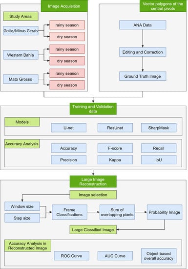
2. Materials and Methods

The image processing included the following steps (Figure 1): (a) Definition of three study areas with a high concentration of CPIS in central Brazil; (b) acquisition of Landsat-8 Operational Land Imager (OLI) images (30-m resolution) considering the seasonal variations of the rain and drought periods; (b) definition of CPIS datasets containing Landsat images and ground truth mask of 256×256 pixels; (c) training stage using three popular CNN architectures (U-net, Deep ResUnet, and SharpMask); (d) large image reconstruction using a sliding window algorithm; (e) analysis of seasonal effects in the detection of CPIS; and (f) accuracy analysis.
In general, object detection is challenging in large remote sensing images, which requires the establishment of reasonable dimensions of the training sample to obtain performance in processing and memory management. The definition of the sample size must consider the characteristics of the object, such as the format, locations, and scales. Thus, a strategy for the classification of a large remote sensing image is to subdivide it into patches with the same size as the training samples and to use a sliding window algorithm with a determined stride (overlap interval between patches). In this context, the present research performs numerous stride length comparisons to identify the optimal parameters to image reconstruction for center-pivot mapping. In addition, the research assesses the effects of phenological variations of natural vegetation and plantations during the rainy and dry period in the CPIS detection process.

2.1. Study Area

The study sites cover three regions of central Brazil, presenting a high concentration of center pivots favored by the flat terrain that allows mechanization: (a) Western Bahia (835 center pivots); (b) Goiás/Minas Gerais (2672 center pivots); and (c) Mato Grosso (224 center pivots) (Figure 2). In these regions, water scarcity between May and September prevents the cultivation of several crops, requiring the need for additional irrigation water.
The Western Bahia region with flat topography and water availability (from the rainfall, rivers, and groundwater) shows an increasing expansion of mechanized farming that replaced traditional agriculture [2,58,59,60,61] and an intensification of the implantation of center pivots [62]. Western Bahia had a significant increase in the irrigated area, ranging from 9 center pivots in 1985 to 1550 center pivots in 2016, which has caused water conflicts since 2010 [63].
The Goiás/Minas Gerais region has one of the highest concentrations of center pivots in Brazil, reaching the number of hundreds. In this region, there is a conflict over the use of water between the sectors of irrigated agriculture, human consumption, and hydroelectric power generation. Several types of research have already been carried out in the mapping of center pivot areas, analysis of areas suitable for the expansion of irrigation, demand for water for irrigation, and conflicts arising from competition for multiple water use [64,65,66,67].
The state of Mato Grosso has favorable environmental factors for agriculture, being one of the leading agricultural producers of soy and corn [68,69,70,71]. Besides, Mato Grosso had the most significant center pivot increase in the 2010–2017 period (175% growth), consolidating itself as an essential Brazilian irrigation center that still has considerable expansion potential [72].

2.2. Dataset and Training Samples

In deep learning techniques, extensive and qualified datasets are critical for object recognition success and meaningful performance comparisons between different algorithms. Satellite images allow the creation of extensive datasets in space and time that capture the vast richness and diversity of objects present on the land surface, which results in high-performance object recognition. The challenge is to establish a dataset contending the satellite images alongside with the corresponding ground truth image. The present research used data from the “Center Pivots in Brazil Irrigated Agriculture Survey”, developed by the National Water Agency (ANA) [3], which contains all the vector data of the center-pivot polygons of the Brazilian territory in 2013/2014. The ANA survey extracted the vector polygons of CPIS from the visual interpretation of Landsat-8 OLI images. The preparation of ground truth images used this ANA database with some minor corrections when necessary.
For data compatibility with the ANA survey, we also used Landsat-8 surface reflectance images [73] from the same year 2014 or 2015 for the training and validation data. In central Brazil, the climate has well-defined rainy and dry seasons, with distinct phenological behaviors [74,75]. This climatic variability is responsible for differences within the same type of vegetation or planting, such as regeneration, vegetative growth, flowering, fruiting, and seed dispersal. Therefore, the image acquisition covered dry and rainy months with the different responses of vegetation and crop. Table 1 lists the set of images used in the three study areas. In the analyzed temporal images, we observed changes in the presence of center pivots in specific locations, even in short periods (Figure 3). Thus, we checked and corrected the center pivot polygons to elaborate on the ground truth images.
This research considered two classes of interest (center pivots and non-pivots). The dataset had 5000 frames of each 256 × 256 pixel (4200 with center pivots and 800 without center pivots) with an 80%–20% train-test split (4000 frames for training and 1000 for validation). We evaluated three different neural network architectures (Deep ResUnet, U-net, and Sharpmask) with the following hyperparameter configurations: (a) 200 epoch training with callbacks, (b) batch size of 8, (c) Adam optimizer, and (d) dice coefficient as the loss function. Additionally, each model’s input layer was adjusted to support seven-channel Landsat images with 256 × 256 dimensions, resulting in a 256 × 256 × 7 input shape. For data processing, we used a computer equipped with a Nvidia GeForce RTX 2080 TI graphic card with 11 GB of GPU memory, 16 GB RAM, and an Intel Core i7–4770K CPU processor with a 3.5 GHz processing speed.

2.3. Deep Learning Models

In this present research, we used three deep learning architectures: U-net [76], Deep ResUnet [77], and SharpMask [78]. U-net achieves significant results in the semantic segmentation, because of its ability to preserve essential features in the image, having two main parts: Contraction and expansion [76]. The name U-net comes from the symmetrical trajectory between both model parts (contraction and expansion) that describes a U-shape architecture. Thus, the U-net model has a series of kernels that act as filters that map specific features. The contraction (encoder) stage of the architecture consists of cascade downsampling, which reduces the image size and increasing the number of filters. The expansive (decoder) stage consists of a symmetrical number of up samples, returning the image to its original size, and decreasing the number of filters to the number of outputs. Each downsampling stage has two Conv2D layers, two batch normalization layers, and two ReLu activation functions, ending with the MaxPooling layer. The upsampling stage has the same format, but instead of the MaxPooling layer at the end, there is an upsampling layer at the beginning. There are five downsamples, which means the image gets to 1/32 of its original size, and five upsamples. The architecture ends with a sigmoid activation function. U-net has been used for the semantic segmentation of targets in remote sensing images: Road network [79], water body [80], building extraction [46,81], raft aquaculture areas [82], and edge-feature-based perceptual hash [83].
The deep residual U-Net (Deep ResUnet) combines the strengths of deep residual learning and the U-Net architecture [77] (https://github.com/nikhilroxtomar/Deep-Residual-Unet). The main advantages of the model are (a) replacement of plain neural units by residual units as a basic block, and (b) removal of cropping operation, allowing better performance because it is unnecessary. The architecture consists of encoder and decoder blocks. The decoder block has three sets of batch normalization, ReLu activation function, padding, and convolutional block. The encoder block has the same structure, but with strides, so the image is downsampled. The architecture ends with a sigmoid activation function. The Deep ResUnet and its variation have been investigated for satellite image segmentation [77,84,85].
Facebook’s SharpMask is a network that enhances the sharpness of segmentation masks to object classification [78], which can be very satisfactory for our case, which deals with geometric objects. The architecture consists of convolutional and refinement blocks composed of three sets of Lambda, Conv2D, batch normalization, and ReLu activation functions. However, the refinement stage also adds activation functions. Every convolutional block is connected to a MaxPooling layer, and every refinement block is connected to an upsampling layer. We performed four convolutional and refinement blocks that connect to a dense layer with 64 neurons and a ReLu activation function, and at the end, the sigmoid activation function. De Bem et al. [48] used SharpMask to detect changes in the Amazon region.

2.4. Classified Image Reconstruction for Large Scenes

We developed a sliding window with the same training image dimension that slides over the image for entire scene classification. Window movement can use different stride values in the horizontal and vertical directions. Figure 4 demonstrates the process of classifying large images from a sliding window. In the example, an 8 × 8 window slides over an image with a stride of two pixels. This process generates an overlap between consecutive frames considering stripe dimensions smaller than the window size (Figure 5). Thus, a set of values may be produced for a pixel that can be used to improve target detection.
The tests conducted in this research considered different stride values between two successive windows. Algorithms to reconstruct large images based on a sliding window with overlapping pixels were applied for remote sensing data. Previous studies used the average values of overlapping pixels to reduce the impact of frame boundaries, which tend to have more errors [48,57]. Instead of using the average, we established a proportionality index of the number of times the pixel was classified as a center pivot. Thus, we increased the pixel counter by one when the result value was greater than 0.7, which means a high probability of having a center pivot. In the end, for each pixel, we had a ratio of the number of times the method identified the pivot divided by the number of overlapping data, restricting the range of values between 0 and 1. The proportionality calculation considers the edge effect in the total image as necessary (Figure 5). A threshold value defines the center pivot and non-center pivot binary image.

2.5. Season Analysis

The central Brazil region presents a substantial phenological variation throughout the year. In the Cerrado biome, water scarcity is the primary climatic determinant of leaf phenology, establishing the period to produce dry leaves and the sprouting of new leaves. The Cerrado vegetation has herbaceous and arboreal strata. Herbaceous plants lose their leaves in the dry season and produce new leaves at the beginning of the rains. Woody plants have different strategies, in which the brevideciduous and deciduous species completely lose their foliage during the dry period, and the evergreen species keep their leaves throughout the year. Besides, the stages of planting cycles also interfere with the detection of CPIS. Therefore, we chose images with different photosynthetic responses from water stress, as shown in Table 2 and Figure 6. The area analyzed was the Goiás/Minas Gerais region, which has the highest concentration of CPIS, encompassing three Landsat scenes. The image with the highest percentage of photosynthetic vegetation was from May 2019, representing the end of the rainy season (Figure 6A). In contrast, the image from the critical dry period (August 2019) has a few areas with photosynthetically active vegetation, limited to some CPIS and riparian forest (Figure 6C). Additionally, we added an image from the beginning of the dry season with intermediate behavior from June 2018 (Figure 6B). One of the most considerable difficulties in obtaining rainy season imagery is the presence of clouds, especially when analyzing large areas.

2.6. Accuracy Assessment

The accuracy analysis is crucial to establish the product quality and to compare classification algorithms. The accuracy assessment for the different methodological approaches adopted 1000 validation samples. We used the metrics commonly used for object detection: Total accuracy, precision, recall, F1, Kappa coefficient, and IoU [86,87,88,89,90]. Table 3 lists the equations for accuracy metrics. Besides, in the evaluation of the image reconstruction with different overlays, we used a new Landsat image (2018) and the ROC-curve analysis.
Finally, we performed an object-based precision analysis to assess the correctness of the number of center pivots, crucial information for public managers [91,92].

3. Results

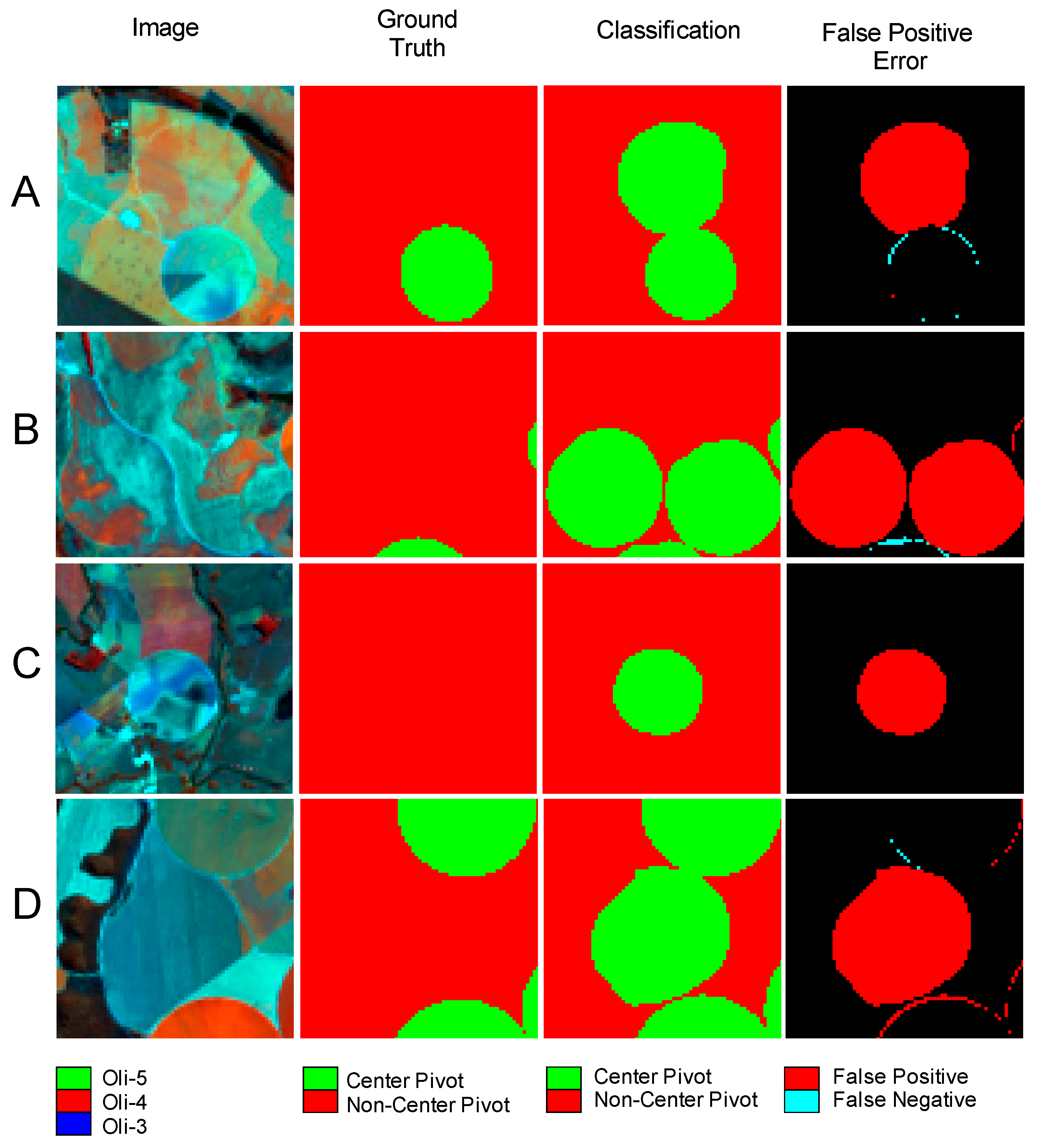
3.1. Comparison between CNN architectures from the validation samples

The training stage obtained low values for losses (< 0.05) and high values for Dice coefficients (> 0.99) for all the three methods, which was very satisfactory, demonstrating a high CPIS detection capacity. The CNN architecture efficiency is due to the great diversity of selected samples. This result indicates that all methods had an excellent ability to perform semantic segmentation for center pivots on multispectral data, considering different crops, shapes, and dimensions.
The accuracy scores had a pixel-wise analysis in the validation set (1000 images), totaling a pixel count of 65,536,000 (256×256×1000). The results demonstrated that the U-net had the best performance within the three networks (Table 4, Figure 7). Even though the results were very similar, the residual blocks present in Deep ResUnet did not improve the performance in comparison to U-net, probably because the target has a constant geometric shape, varying only in size. Therefore, this result shows that simpler structures are sufficient for our analysis.

3.2. Results of Entire Classified Image in Different Seasons

Segmentation within independent frames tends to have more errors at their edges [57]. Therefore, the image reconstruction from the classified frames with overlapping pixels can minimize these errors. To assess the overlap effect on the result, we selected our best model (U-net) and six different stride values (8, 16, 32, 64, 128, 256). This procedure used three independent Landsat images with 2560 × 2560-pixel dimensions from the Goiás/Minas Gerais region on 18 June 2018, 20 May 2019, and 24 August 2019. As expected, images with fewer overlapping pixels had a lot of errors at the frame edges, while increasing the number of overlapping pixels resulted in well-marked pivots, significantly minimizing errors.
The image reconstruction from the sliding windows with overlapping pixels had a significant improvement in classification (Figure 8). The probability image became much closer to the ground truth image, with the stride value decreasing. Another interesting point is the precision of the method when analyzing the variety of spectral behaviors, texture, and internal arrangement within each center pivot. These nuances are complicated even for human recognition, evidencing the importance and precision in the automatic classification of CPIS. Despite all the benefits with stride reduction, a considerable disadvantage of the overlapping windows technique is the longer processing time. Reducing the stride value by half on the x and y axes increased the classification time by four times. Image classification with no overlapping pixels is a fast task while using low stride values is a long process. The classification in a 2560 × 2560-pixel image with no overlapping pixels took about 30 s to complete, while using a stride value of eight took about nine hours. Figure 8 shows the procedures to generate the classified binary image from the probability image.
We obtained the optimal threshold for CPIS detection by testing a succession of threshold values and chose the one with the greater Kappa coefficient when compared to its ground truth image [93]. These successive comparisons generated a graphical overview of Kappa’s trajectory with threshold values from 0 to 1 (Figure 9A1,B1,C1). This quantitative method reduces subjectivity in defining the optimal threshold value. The low optimal thresholds are due to the high selectivity of the index, weighing in favor of high activation pixels, and demonstrating a good likelihood to be a center pivot. The low threshold value reveals that the index produces a reduction of noisy points in the image, bringing a lower rate of false negatives.
To evaluate the different stride values in the three distinct dates, we used the receiving operating characteristic curve (ROC) in a pixel-wise analysis presented in Figure 10. The ROC curve is a graphical representation of how well the model can differentiate two classes, by comparing two axes: (a) False positive rate (FPR) and (b) true positive rate (TPR). The closer to 1 in the area under the curve (AUC), the better the model performs. Additionally, the comparison of ROC curves from different periods is an interesting analysis because it shows how well the models can differentiate classes with different inputs. As expected, the areas with more significant photosynthetically active vegetation had better results (rainy and beginning of the dry season), while the critical dry period had weaker results. Stride value reduction increased the AUC scores in all three scenarios, achieving the highest value in the intermediate period (B) (0.984). In the rainy season (A), the results had a similar behavior compared to the intermediate period, with slightly lower values. The critical dry season (C) had the most different response since the reconstruction without overlapping pixels had significantly worse outcomes than the other two periods, but stride reduction significantly increased the ability to differentiate classes in a pixel-wise analysis.
The pixel-wise accuracy analysis presented similar results for the three dates. To make a better differentiation, we performed an object-based accuracy approach for the three Landsat images (2560 × 2560 pixels). This information is vital for public managers who seek to estimate the number of CPIS and evaluate the best scenarios to identify the center pivots. Table 5 lists the confusion matrix of the three dates. We identified: (a) 937 from 974 center pivots at the beginning of the dry season (96% OA); (b) 902 from 974 center pivots at the end of the rainy season (92% OA); and (c) 860 from 974 center pivots at the end of the dry season (88% OA). Even though the pixel-wise analysis had similar results, the object-based analysis shows a great difference within the three periods.
Results from the beginning of the dry season had significantly better results than the rainy and critical dry period. Although the errors encountered in the classification of center pivots are due to their similarity with the surroundings, the source of the error is different. In the rainy season, the vegetation’s photosynthetically active areas became very similar to the center pivots that have crop development. In contrast, in the critical dry period, harvesting associated with the conservation tillage practice in reducing runoff and erosion has a similar reflectance with the dry vegetation. Figure 11 shows zoomed areas from the Goiás/Minas Gerais region within the three different dates showing areas that had correct classifications only in the beginning of the dry period. In the rainy season, the red color associated with the photosynthetically active vegetation shows that the center pivot and its surroundings had similar spectral behaviors. Likewise, in the critical dry period, non-photosynthetically active vegetation takes on a white color, homogenizing the CPIS with adjacent areas.
Figure 12 shows locations where only the images of the beginning of the dry season detected CPIS. The photosynthetically active vegetation is now gone, and the center pivots have very similar behavior with its dry surrounding. Additionally, this kind of error is much more common than rainy season errors. The present research shows that the identification in the intermediate season is optimal since it has the advantage of photosynthetically active regions inside the pivots, but without the similarity with the vegetation surroundings.
Figure 13 shows a rare situation where only the center pivots present in the rainy season image were correctly identified. The pattern of non-recognition was the same as the previous ones, having very similar environments around it. Figure 13B also presents a center pivot that was not identified in any of the periods.
Figure 14 shows that most center pivots classified as false positives had significant similarities with the class of interest, being a controversial detection task even to specialized professionals. Figure 14A–C present a possible case of abandoned center pivots, due to the lack of planting area within the circular shape. Figure 14D illustrates a polygon that was erroneously mapped but has a similar center pivot shape. We can observe that even the errors obtained from the predictions are very hard to determine, ensuring state-of-the-art results to this classification problem. Besides, the error images (Figure 12) also demonstrate an increase in errors along the circumference of the CPIS, being a predictable result, since the manual classification hardly achieves standardization, such as automatic classification. Therefore, this type of effect should not be considered an incorrect classification.

4. Discussion

The present research shows state-of-the-art image segmentation results with high accuracy for CPIS detection in all deep learning models analyzed. This approach has a significant contribution to faster CPIS identification when compared to visual interpretation mapping. The vast majority of CPIS inventories consist of visual interpretation of circular shapes from satellite images. Rundquist et al. [19] systematized 14 years of CPIS inventory in Nebraska. The authors found that dry conditions in Nebraska’s state promoted a marked growth of CPIS during the period studied. Schmidt et al. [34] carried out the mapping of the CPIS for Brazil’s southeastern region in 2002. The research found a total of 4134 CPIS, considering an error greater than 5% due to cloud interference and lack of contrast between the irrigated area and its surroundings. Sano et al. [33] assessed the growth of CPIS in the Federal District of Brazil in the period 1992–2002 to estimate water demand. In the 20 years, the number of center pivots grew from 55 to 104. Ferreira et al. [32] mapped 3781 CPIS in the State of Minas Gerais (Brazil) for the year 2008 using images from the China-Brazil Earth-Resources Satellite 2B / Couple Charged Device (CBERS2B / CCD) satellite. The most significant survey was conducted by the National Water Agency [3], which mapped the entire Brazilian territory in 2004, the data used in this survey.
U-net had slightly better metrics for our target compared to Deep ResUnet, contrasting with other segmentation studies with different targets [48,57,77]. De Bem et al. [48] compared these networks in deforest change detection and obtained better Kappa results for ResUnet (0.94) over U-net (0.91). In urban building detection, Yi et al. [57] also had better Kappa results for Deep ResUnet (0.9176) over U-net (0.8709). Zhang et al. [77] in road extraction analysis used precision-recall breakeven points to evaluate the performance of the models, obtaining closer values between Deep ResUnet (0.9187) and U-net (0.9053). Similarities between Deep ResUnet and U-net results in the present research are probably associated with the trained data. Differences in our data include seven-channel imagery and circular-shaped targets, which can provide simpler structures, showing the similarity between the methods. Even though SharpMask brings the worst accuracy performance, one advantage when compared to the other two networks is the faster training period.
The verified errors occur mostly in different border areas: (a) At the edge of the entire classification due to a smaller amount of overlapping pixels; (b) at the edge of the frames, because the geometric shape of the center pivots only appears partially; and (c) along the circumference of the center pivot, because there are small divergences in the manual labels and the classified image. Previous research in the large image segmentation used the overlapping pixel values from the sliding window to attenuate frame edge errors [48,57]. A methodological novelty was a quantitative analysis by ROC and AUC to analyze the improvement in accuracy with the increase of the overlap area. We also proposed an index for the overlap data, considering the proportion of times the value was greater than 70%. In future research, errors of a semantic nature, such as the classification of abandoned center pivots, can be minimized with the use of a time series due to the ability to detect phenological changes in plantations.

5. Conclusions

This research focused on the detection of center pivots from three study areas in central Brazil, considering (a) the development of an extensive center pivot database that encompasses different environments in central Brazil and seasonal changes; (b) evaluation of three models based on CNN architecture; and (c) assessment of the procedure for image reconstruction, considering different variations of overlapping ranges. The results achieved state-of-the-art metrics, with the identification of nearly all center pivots. The training and test dataset had 5000 frames that used ground truth information from visual interpretation of the images, which guaranteed quality information and enriched the model’s quality. The classification methods using U-net, Deep ResUnet, and SharpMask reached high values for the different accuracy metrics (total accuracy > 0.97, F-Score > 0.93, Recall > 0.90, Precision > 0.96, Kappa > 0.92, and IoU > 0.87). U-net had a slight advantage over Deep ResUnet. A significant contribution of this research was the image reconstruction proposition for large images, considering different stride values for the moving window, allowing several classified image overlays and a better pivot estimation per pixel. This procedure enables improvements in the final image. The results show that moving windows with little or lower overlapping pixels have significant errors at the edges of the frames, but also we identified a significant tradeoff when considering the execution time: No overlapping pixels is a 30 s task while using a large number of overlapping pixels is a task that takes nearly 9 h. This performance could be improved using better GPU processors. Although we already expected better results with stride reduction, the present research conducted a quantitative analysis of this improvement. Classification using deep semantic segmentation is essential, as it replaces manual labor and increases speed. Another crucial information in this research was the seasonal analysis, which is evidence that the best time to identify the presence of center pivots is at the beginning of the dry season since it shows greater contrast with its surroundings, identifying nearly all center pivots present in the scene. This information has implications for agrarian and water management, energy consumption, and land use planning. Future studies should include the development of specific neural networks and test images of different sizes to see if the frame’s training size has an impact on the result.

Author Contributions

Conceptualization, A.O.d.A., O.A.d.C.J., O.L.F.d.C., and P.P.d.B.; methodology, A.O.d.A., O.A.d.C.J., O.L.F.d.C., P.P.d.B.; software, C.R.S., O.L.F.d.C., P.H.G.F., P.P.d.B., R.d.S.d.M.; validation, A.O.d.A., C.R.S., O.L.F.d.C., and P.H.G.F.; formal analysis, O.A.d.C.J., P.H.G.F., R.F.G.; investigation, R.F.G., P.H.G.F.; resources, O.A.d.C.J., R.A.T.G., R.F.G.; data curation, A.O.d.A., O.L.F.d.C., P.H.G.F.; writing—original draft preparation, A.O.d.A., O.A.d.C.J., O.L.F.d.C., R.F.G; writing—review and editing, O.A.d.C.J., R.A.T.G., R.F.G. R.d.S.d.M; supervision, O.A.d.C.J., R.A.T.G., R.F.G.; project administration, O.A.d.C.J., R.A.T.G., R.F.G.; funding acquisition, O.A.d.C.J., R.A.T.G., R.F.G. All authors have read and agreed to the published version of the manuscript.

Funding

This research was funded by the following institutions: National Council for Scientific and Technological Development (434838/2018-7), Coordination for the Improvement of Higher Education Personnel and the Union Heritage Secretariat of the Ministry of Economy.

Acknowledgments

The authors are grateful for financial support from CNPq fellowship (Osmar Abílio de Carvalho Júnior, Roberto Arnaldo Trancoso Gomes, and Renato Fontes Guimarães). Special thanks are given to the research group of the Laboratory of Spatial Information System of the University of Brasilia for technical support. The authors thank the researchers form the Union Heritage Secretariat of the Ministry of Economy, who encouraged research with deep learning. This study was financed in part by the Coordination for the Improvement of Higher Education Personnel (CAPES) – Finance Code 001. Finally, the authors acknowledge the contribution of anonymous reviewers.

Conflicts of Interest

The authors declare no conflict of interest.

References

  1. Alexandridis, T.K.; Zalidis, G.C.; Silleos, N.G. Mapping irrigated area in Mediterranean basins using low cost satellite Earth Observation. Comput. Electron. Agric. 2008, 64, 93–103. [Google Scholar] [CrossRef]
  2. Althoff, D.; Rodrigues, L.N. The expansion of center-pivot irrigation in the Cerrado biome. IRRIGA 2019, 1, 56–61. [Google Scholar] [CrossRef]
  3. Agência Nacional de Águas (Brasil). Levantamento da Agricultura Irrigada por Pivôs Centrais no Brasil—2014: Relatório Síntese; Agência Nacional de Águas (ANA): Brasília, Brasil, 2016; ISBN 978-85-8210-034-9. [Google Scholar]
  4. Alexandratos, N.; Bruinsma, J. World Agriculture towards 2030/2050: The 2012 Revision; No. 12-03, ESAWorking Paper; FAO, Agricultural Development Economics Division: Rome, Italy, 2012. [Google Scholar]
  5. Siebert, S.; Döll, P. Quantifying blue and green virtual water contents in global crop production as well as potential production losses without irrigation. J. Hydrol. 2010, 384, 198–217. [Google Scholar] [CrossRef]
  6. Crist, E.; Mora, C.; Engelman, R. The interaction of human population, food production, and biodiversity protection. Science 2017, 356, 260–264. [Google Scholar] [CrossRef] [PubMed]
  7. Aznar-Sánchez, J.A.; Belmonte-Ureña, L.J.; Velasco-Muñoz, J.F.; Manzano-Agugliaro, F. Economic analysis of sustainable water use: A review of worldwide research. J. Clean. Prod. 2018, 198, 1120–1132. [Google Scholar] [CrossRef]
  8. Mancosu, N.; Snyder, R.L.; Kyriakakis, G.; Spano, D. Water scarcity and future challenges for food production. Water 2015, 7, 975–992. [Google Scholar] [CrossRef]
  9. Velasco-Muñoz, J.F.; Aznar-Sánchez, J.A.; Batlles-delaFuente, A.; Fidelibus, M.D. Sustainable irrigation in agriculture: An analysis of global research. Water 2019, 11, 1758. [Google Scholar] [CrossRef] [Green Version]
  10. Velasco-Muñoz, J.F.; Aznar-Sánchez, J.A.; Belmonte-Ureña, L.J.; López-Serrano, M.J. Advances in water use efficiency in agriculture: A bibliometric analysis. Water 2018, 10, 377. [Google Scholar] [CrossRef] [Green Version]
  11. Velasco-Muñoz, J.V.; Aznar-Sánchez, J.A.; Belmonte-Ureña, L.J.; Román-Sánchez, I.M. Sustainable water use in agriculture: A review of worldwide research. Sustainability 2018, 10, 1084. [Google Scholar] [CrossRef] [Green Version]
  12. Cotterman, K.A.; Kendall, A.D.; Basso, B.; Hyndman, D.W. Groundwater depletion and climate change: Future prospects of crop production in the Central High Plains Aquifer. Clim. Chang. 2018, 146, 187–200. [Google Scholar] [CrossRef]
  13. Myers, S.S.; Smith, M.R.; Guth, S.; Golden, C.D.; Vaitla, B.; Mueller, N.D.; Dangour, A.D.; Huybers, P. Climate change and global food systems: Potential impacts on food security and undernutrition. Annu. Rev. Public Health 2017, 38, 259–277. [Google Scholar] [CrossRef] [PubMed]
  14. Ambast, S.K.; Keshari, A.K.; Gosain, A.K. Satellite remote sensing to support management of irrigation systems: Concepts and approaches. Irrig. Drain. 2002, 51, 25–39. [Google Scholar] [CrossRef]
  15. Ozdogan, M.; Yang, Y.; Allez, G.; Cervantes, C. Remote sensing of irrigated agriculture: Opportunities and challenges. Remote Sens. 2010, 2, 2274–2304. [Google Scholar] [CrossRef] [Green Version]
  16. Thenkabail, P.S.; Hanjra, M.A.; Dheeravath, V.; Gumma, M. A Holistic view of global croplands and their water use for ensuring global food security in the 21st century through advanced remote sensing and non-remote sensing approaches. Remote Sens. 2010, 2, 211–261. [Google Scholar] [CrossRef] [Green Version]
  17. Davis, K.F.; Rulli, M.C.; Seveso, A.; D’Odorico, P. Increased food production and reduced water use through optimized crop distribution. Nat. Geosci. 2017, 10, 919–924. [Google Scholar] [CrossRef]
  18. Heller, R.C.; Johnson, K.A. Estimating irrigated land acreage from Landsat imagery. Photogramm. Eng. Remote Sens. 1979, 45, 1379–1386. [Google Scholar]
  19. Rundquist, D.C.; Hoffman, R.O.; Carlson, M.P.; Cook, A.E. The Nebraska Center-Pivot Inventory: An example of operational satellite remote sensing on a long-term basis. Photogramm. Eng. Remote Sens. 1989, 55, 587–590. [Google Scholar]
  20. Chen, Y.; Lu, D.; Luo, L.; Pokhrel, Y.; Deb, K.; Huang, J.; Ran, Y. Detecting irrigation extent, frequency, and timing in a heterogeneous arid agricultural region using MODIS time series, Landsat imagery, and ancillary data. Remote Sens. Environ. 2018, 204, 197–211. [Google Scholar] [CrossRef]
  21. Ozdogan, M.; Gutman, G. A new methodology to map irrigated areas using multi-temporal MODIS and ancillary data: An application example in the continental US. Remote Sens. Environ. 2008, 112, 3520–3537. [Google Scholar] [CrossRef] [Green Version]
  22. Pervez, M.S.; Brown, J.F. Mapping irrigated lands at 250-m scale by merging MODIS data and national agricultural statistics. Remote Sens. 2010, 2, 2388–2412. [Google Scholar] [CrossRef] [Green Version]
  23. Pervez, M.S.; Budde, M.; Rowland, J. Mapping irrigated areas in Afghanistan over the past decade using MODIS NDVI. Remote Sens. Environ. 2014, 149, 155–165. [Google Scholar] [CrossRef] [Green Version]
  24. Bazzi, H.; Baghdadi, N.; Ienco, D.; El Hajj, M.; Zribi, M.; Belhouchette, H.; Escorihuela, M.J.; Demarez, V. Mapping irrigated areas using Sentinel-1 time series in Catalonia, Spain. Remote Sens. 2019, 11, 1836. [Google Scholar] [CrossRef] [Green Version]
  25. Bazzi, H.; Baghdadi, N.; El Hajj, M.; Zribi, M.; Minh, D.H.T.; Ndikumana, E.; Courault, D.; Belhouchette, H. Mapping paddy rice using Sentinel-1 SAR time series in Camargue, France. Remote Sens. 2019, 11, 887. [Google Scholar] [CrossRef] [Green Version]
  26. Bousbih, S.; Zribi, M.; El Hajj, M.; Baghdadi, N.; Lili-Chabaane, Z.; Gao, Q.; Fanise, P. Soil Moisture and Irrigation Mapping in a semi-arid region, based on the synergetic use of Sentinel-1 and Sentinel-2 Data. Remote Sens. 2018, 10, 1953. [Google Scholar] [CrossRef] [Green Version]
  27. Gao, Q.; Zribi, M.; Escorihuela, M.; Baghdadi, N.; Segui, P. Irrigation mapping using Sentinel-1 time series at field scale. Remote Sens. 2018, 10, 1495. [Google Scholar] [CrossRef] [Green Version]
  28. Demarez, V.; Helen, F.; Marais-Sicre, C.; Baup, F. In-season mapping of irrigated crops using Landsat 8 and Sentinel-1 time series. Remote Sens. 2019, 11, 118. [Google Scholar] [CrossRef] [Green Version]
  29. Fieuzal, R.; Duchemin, B.; Jarlan, L.; Zribi, M.; Baup, F.; Merlin, O.; Hagolle, O.; Garatuza-Payan, J. Combined use of optical and radar satellite data for the monitoring of irrigation and soil moisture of wheat crops. Hydrol. Earth Syst. Sci. 2011, 15, 1117–1129. [Google Scholar] [CrossRef] [Green Version]
  30. Hadria, R.; Duchemin, B.; Jarlan, L.; Dedieu, G.; Baup, F.; Khabba, S.; Olioso, A.; Le Toan, T. Potentiality of optical and radar satellite data at high spatio-temporal resolutions for the monitoring of irrigated wheat crops in Morocco. Int. J. Appl. Earth Obs. Geoinf. 2010, 12, S32–S37. [Google Scholar] [CrossRef]
  31. Martins, J.D.; Bohrz, I.S.; Tura, E.F.; Fredrich, M.; Veronez, R.P.; Kunz, G.A. Levantamento da área irrigada por pivô central no Estado do Rio Grande do Sul. IRRIGA 2016, 21, 300. [Google Scholar] [CrossRef]
  32. Ferreira, E.; Toledo, J.H.D.; Dantas, A.A.; Pereira, R.M. Cadastral maps of irrigated areas by center pivots in the State of Minas Gerais, using CBERS-2B/CCD satellite imaging. Eng. Agríc 2011, 31, 771–780. [Google Scholar] [CrossRef] [Green Version]
  33. Sano, E.E.; Lima, J.E.; Silva, E.M.; Oliveira, E.C. Estimative variation in the water demand for irrigation by center pivot in Distrito Federal-Brazil, between 1992 and 2002. Eng. Agríc. 2005, 25, 508–515. [Google Scholar] [CrossRef] [Green Version]
  34. Schmidt, W.; Coelho, R.D.; Jacomazzi, M.A.; Antunes, M.A. Spatial distribution of center pivots in Brazil: I-southeast region. Rev. Bras. Eng. Agríc. Ambient. 2004, 8, 330–333. [Google Scholar] [CrossRef] [Green Version]
  35. Garcia-Garcia, A.; Orts-Escolano, S.; Oprea, S.; Villena-Martinez, V.; Garcia-Rodriguez, J. A review on deep learning techniques applied to semantic segmentation. arXiv 2017, arXiv:1704.06857. [Google Scholar]
  36. Garcia-Garcia, A.; Orts-Escolano, S.; Oprea, S.; Villena-Martinez, V.; Martinez-Gonzalez, P.; Garcia-Rodriguez, J. A survey on deep learning techniques for image and video semantic segmentation. Appl. Soft Comput. 2018, 70, 41–65. [Google Scholar] [CrossRef]
  37. Guo, Y.; Liu, Y.; Georgiou, T.; Lew, M.S. A review of semantic segmentation using deep neural networks. Int. J. Multimed. Inf. Retr. 2018, 7, 87–93. [Google Scholar] [CrossRef] [Green Version]
  38. Guo, Y.; Liu, Y.; Oerlemans, A.; Lao, S.; Wu, S.; Lew, M.S. Deep learning for visual understanding: A review. Neurocomputing 2016, 187, 27–48. [Google Scholar] [CrossRef]
  39. Ma, L.; Liu, Y.; Zhang, X.; Ye, Y.; Yin, G.; Johnson, B.A. Deep learning in remote sensing applications: A meta-analysis and review. ISPRS J. Photogramm. Remote Sens. 2019, 152, 166–177. [Google Scholar] [CrossRef]
  40. Carranza-García, M.; García-Gutiérrez, J.; Riquelme, J. A framework for evaluating land use and land cover classification using convolutional neural networks. Remote Sens. 2019, 11, 274. [Google Scholar] [CrossRef] [Green Version]
  41. Kussul, N.; Lavreniuk, M.; Skakun, S.; Shelestov, A. Deep Learning Classification of Land Cover and Crop Types Using Remote Sensing Data. IEEE Geosci. Remote Sens. Lett. 2017, 14, 778–782. [Google Scholar] [CrossRef]
  42. Li, M.; Wang, L.; Wang, J.; Li, X.; She, J. Comparison of land use classification based on convolutional neural network. J. Appl. Remote Sens. 2020, 14, 1. [Google Scholar] [CrossRef]
  43. Scott, G.J.; England, M.R.; Starms, W.A.; Marcum, R.A.; Davis, C.H. Training deep convolutional neural networks for land–cover classification of high-resolution imagery. IEEE Geosci. Remote Sens. Lett. 2017, 14, 549–553. [Google Scholar] [CrossRef]
  44. Li, W.; Liu, H.; Wang, Y.; Li, Z.; Jia, Y.; Gui, G. Deep learning-based classification methods for remote sensing images in urban built-up areas. IEEE Access 2019, 7, 36274–36284. [Google Scholar] [CrossRef]
  45. Huang, B.; Zhao, B.; Song, Y. Urban land-use mapping using a deep convolutional neural network with high spatial resolution multispectral remote sensing imagery. Remote Sens. Environ. 2018, 214, 73–86. [Google Scholar] [CrossRef]
  46. Xu, Y.; Wu, L.; Xie, Z.; Chen, Z. Building extraction in very high resolution remote sensing imagery using deep learning and guided filters. Remote Sens. 2018, 10, 144. [Google Scholar] [CrossRef] [Green Version]
  47. Wagner, F.H.; Dalagnol, R.; Tarabalka, Y.; Segantine, T.Y.F.; Thomé, R.; Hirye, M.C.M. U-Net-Id, an Instance Segmentation Model for Building Extraction from Satellite Images—Case Study in the Joanópolis City, Brazil. Remote Sens. 2020, 12, 1544. [Google Scholar] [CrossRef]
  48. De Bem, P.P.; de Carvalho Junior, O.A.; Fontes Guimarães, R.; Trancoso Gomes, R.A. Change detection of deforestation in the Brazilian Amazon using Landsat data and Convolutional Neural Networks. Remote Sens. 2020, 12, 901. [Google Scholar] [CrossRef] [Green Version]
  49. Ma, W.; Xiong, Y.; Wu, Y.; Yang, H.; Zhang, X.; Jiao, L. Change detection in remote sensing images based on image mapping and a deep capsule network. Remote Sens. 2019, 11, 626. [Google Scholar] [CrossRef] [Green Version]
  50. Peng, D.; Zhang, Y.; Guan, H. End-to-end change detection for high resolution satellite images using improved UNet++. Remote Sens. 2019, 11, 1382. [Google Scholar] [CrossRef] [Green Version]
  51. Zhang, W.; Lu, X. The spectral-spatial joint learning for change detection in multispectral imagery. Remote Sens. 2019, 11, 240. [Google Scholar] [CrossRef] [Green Version]
  52. Chen, Y.; Fan, R.; Bilal, M.; Yang, X.; Wang, J.; Li, W. Multilevel Cloud detection for high-resolution remote sensing imagery using multiple convolutional neural networks. ISPRS Int. J. Geo-Inf. 2018, 7, 181. [Google Scholar] [CrossRef] [Green Version]
  53. Jeppesen, J.H.; Jacobsen, R.H.; Inceoglu, F.; Toftegaard, T.S. A cloud detection algorithm for satellite imagery based on deep learning. Remote Sens. Environ. 2019, 229, 247–259. [Google Scholar] [CrossRef]
  54. Li, Z.; Shen, H.; Cheng, Q.; Liu, Y.; You, S.; He, Z. Deep learning-based cloud detection for medium and high-resolution remote sensing images of different sensors. ISPRS J. Photogramm. Remote Sens. 2019, 150, 197–212. [Google Scholar] [CrossRef] [Green Version]
  55. Xie, F.; Shi, M.; Shi, Z.; Yin, J.; Zhao, D. Multilevel cloud detection in remote sensing images based on deep learning. IEEE J. Sel. Top. Appl. Earth Obs. Remote Sens. 2017, 10, 3631–3640. [Google Scholar] [CrossRef]
  56. Zhang, C.; Yue, P.; Di, L.; Wu, Z. Automatic identification of center pivot irrigation systems from Landsat images using Convolutional Neural Networks. Agriculture 2018, 8, 147. [Google Scholar] [CrossRef] [Green Version]
  57. Yi, Y.; Zhang, Z.; Zhang, W.; Zhang, C.; Li, W.; Zhao, T. Semantic Segmentation of Urban Buildings from VHR Remote Sensing Imagery Using a Deep Convolutional Neural Network. Remote Sens. 2019, 11, 1774. [Google Scholar] [CrossRef] [Green Version]
  58. Hessel, F.O.; Carvalho Junior, O.A.; Gomes, R.A.T.; Martins, E.S.; Guimarães, R.F. Dinâmica e sucessão dos padrões da paisagem agrícola no município de Cocos (Bahia). RAE GA 2012, 26, 128–156. [Google Scholar] [CrossRef] [Green Version]
  59. De Oliveira, S.N.; Carvalho Júnior, O.A.; Gomes, R.A.T.; Guimarães, R.F.; Martins, E.S. Detecção de mudança do uso e cobertura da terra usando o método de pós-classificação na fronteira agrícola do Oeste da Bahia sobre o Grupo Urucuia durante o período 1988–2011. Rev. Bras. Cartogr. 2014, 66, 1157–1176. [Google Scholar]
  60. De Oliveira, S.N.; Carvalho Júnior, O.A.; Gomes, R.A.T.; Guimarães, R.F.; McManus, C.M. Landscape-fragmentation change detection from agricultural expansion in the Brazilian savanna, Western Bahia, Brazil (1988–2011). Reg. Environ. Chang. 2015, 17, 411–423. [Google Scholar] [CrossRef]
  61. De Oliveira, S.N.; de Carvalho Júnior, O.A.; Gomes, R.A.T.; Guimarães, R.F.; McManus, C.M. Deforestation analysis in protected areas and scenario simulation for structural corridors in the agricultural frontier of Western Bahia, Brazil. Land Use Policy 2017, 61, 40–52. [Google Scholar] [CrossRef]
  62. Menke, A.B.; Carvalho Júnior, O.A.; Gomes, R.A.T.; Martins, E.S.; Oliveira, S.N. Análise das mudanças do uso agrícola da terra a partir de dados de sensoriamento remoto multitemporal no município de Luís EduardoMagalhães (BA–Brasil). Soc. Nat. 2009, 21, 315–326. [Google Scholar] [CrossRef] [Green Version]
  63. Pousa, R.; Costa, M.H.; Pimenta, F.M.; Fontes, V.C.; Brito, V.F.A.; Castro, M. Climate Change and Intense Irrigation Growth in Western Bahia, Brazil: The Urgent Need for Hydroclimatic Monitoring. Water 2019, 11, 933. [Google Scholar] [CrossRef] [Green Version]
  64. Brunckhorst, A.; Bias, E. Aplicação de SIG na gestão de conflitos pelo uso da água na porção goiana da bacia hidrográfica do rio São Marcos, município de Cristalina–GO. Geociências 2014, 33, 228–243. [Google Scholar]
  65. Pinhati, F.S.C. Simulações de ampliações da irrigação por Pivô Central na Bacia do Rio São Marcos. Master’s Thesis, University of Brasília, Brasília, Brazil, 2018. [Google Scholar]
  66. Sano, E.E.; Lima, J.E.F.W.; Silva, E.M.; Oliveira, E.C. Estimativa da Variação na Demanda de Água para Irrigação por Pivô-Central no Distrito Federal entre 1992 e 2002. Eng. Agríc. 2005, 25, 508–515. [Google Scholar] [CrossRef] [Green Version]
  67. Silva, L.M.C.; da Hora, M.A.G.M. Conflito pelo uso da água na bacia hidrográfica do rio São Marcos: O estudo de caso da UHE batalha. Engevista 2015, 17, 166–174. [Google Scholar] [CrossRef] [Green Version]
  68. Galford, G.L.; Mustard, J.F.; Melillo, J.; Gendrin, A.; Cerri, C.C.; Cerri, C.E.P. Wavelet analysis of MODIS time series to detect expansion and intensification of row-crop agriculture in Brazil. Remote Sens. Environ. 2008, 112, 576–587. [Google Scholar] [CrossRef]
  69. Arvor, D.; Jonathan, M.; Meirelles, M.S.P.; Dubreuil, V.; Durieux, L. Classification of MODIS EVI time series for crop mapping in the state of Mato Grosso, Brazil. Int. J. Remote Sens. 2011, 32, 7847–7871. [Google Scholar] [CrossRef]
  70. Bernardes, T.; Adami, M.; Formaggio, A.R.; Moreira, M.A.; de Azeredo França, D.; de Novaes, M.R. Imagens mono e multitemporais MODIS para estimativa da área com soja no Estado de Mato Grosso. Pesqui. Agropecu. Bras. 2011, 46, 1530–1537. [Google Scholar] [CrossRef]
  71. Gusso, A.; Arvor, D.; Ricardo Ducati, J.; Veronez, M.R.; Da Silveira, L.G. Assessing the modis crop detection algorithm for soybean crop area mapping and expansion in the Mato Grosso state, Brazil. Sci. World J. 2014, 2014, 863141. [Google Scholar] [CrossRef]
  72. Agência Nacional de Águas (Brasil). Levantamento da Agricultura Irrigada por Pivôs Centrais no BRASIL/Agência Nacional de Águas, Embrapa Milho e Sorgo, 2nd ed.; ANA: Brasília, Brazil, 2019. [Google Scholar]
  73. Vermote, E.; Justice, C.; Claverie, M.; Franch, B. Preliminary analysis of the performance of the Landsat 8/OLI land surface reflectance product. Remote Sens. Environ. 2016, 185, 46–56. [Google Scholar] [CrossRef]
  74. Abade, N.A.; Carvalho Júnior, O.A.; Guimarães, R.F.; De Oliveira, S.N. Comparative Analysis of MODIS Time-Series Classification Using Support Vector Machines and Methods Based upon Distance and Similarity Measures in the Brazilian Cerrado-Caatinga Boundary. Remote Sens. 2015, 7, 12160–12191. [Google Scholar] [CrossRef] [Green Version]
  75. Carvalho Júnior, O.A.; Sampaio, C.D.S.; Silva, N.C.D.; Couto Júnior, A.F.; Gomes, R.A.T.; Carvalho, A.P.F.; Shimabukuro, Y.E. Classificação de padrões de savana usando assinaturas temporais NDVI do sensor MODIS no Parque Nacional Chapada dos Veadeiros. Rev. Bras. Geof. 2008, 26, 505–517. [Google Scholar] [CrossRef] [Green Version]
  76. Ronneberger, O.; Fischer, P.; Brox, T. U-Net: Convolutional networks for biomedical image segmentation. arXiv 2015, arXiv:1505.04597. [Google Scholar]
  77. Zhang, Z.; Liu, Q.; Wang, Y. Road extraction by deep residual U-Net. IEEE Geosci. Remote Sens. Lett. 2018, 15, 749–753. [Google Scholar] [CrossRef] [Green Version]
  78. Pinheiro, P.O.; Lin, T.Y.; Collobert, R.; Dollár, P. Learning to Refine Object Segments. In Lecture Notes in Computer Science, Proceedings of the Computer Vision–ECCV 2016, Amsterdam, The Netherlands, 11–14 October 2016; Leibe, B., Matas, J., Sebe, N., Welling, M., Eds.; Springer: Cham, Switzerland, 2016; v. 9905; pp. 75–91. [Google Scholar]
  79. He, H.; Yang, D.; Wang, S.; Wang, S.; Li, Y. Road Extraction by Using Atrous Spatial Pyramid Pooling Integrated Encoder-Decoder Network and Structural Similarity Loss. Remote Sens. 2019, 11, 1015. [Google Scholar] [CrossRef] [Green Version]
  80. Feng, W.; Sui, H.; Huang, W.; Xu, C.; An, K. Water body extraction from very high-resolution remote sensing imagery using deep U-Net and a superpixel-based conditional random field model. IEEE Geosci. Remote Sens. Lett. 2018, 16, 618–622. [Google Scholar] [CrossRef]
  81. Li, W.; He, C.; Fang, J.; Zheng, J.; Fu, H.; Yu, L. Semantic Segmentation-Based Building Footprint Extraction Using Very High-Resolution Satellite Images and Multi-Source GIS Data. Remote Sens. 2019, 11, 403. [Google Scholar] [CrossRef] [Green Version]
  82. Cui, B.; Fei, D.; Shao, G.; Lu, Y.; Chu, J. Extracting Raft Aquaculture Areas from Remote Sensing Images via an Improved U-Net with a PSE Structure. Remote Sens. 2019, 11, 2053. [Google Scholar] [CrossRef] [Green Version]
  83. Ding, K.; Yang, Z.; Wang, Y.; Liu, Y. An Improved Perceptual Hash Algorithm Based on U-Net for the Authentication of High-Resolution Remote Sensing Image. Appl. Sci. 2019, 9, 2972. [Google Scholar] [CrossRef] [Green Version]
  84. Liu, Z.; Feng, R.; Wang, L.; Zhong, Y.; Cao, L. D-Resunet: Resunet and Dilated Convolution for High Resolution Satellite Imagery Road Extraction. In Proceedings of the 2019 IEEE International Geoscience and Remote Sensing Symposium—IGARSS 2019, Yokohama, Japan, 28 July–2 August 2109; pp. 3927–3930. [Google Scholar]
  85. Diakogiannis, F.I.; Waldner, F.; Caccetta, P.; Wu, C. Resunet-a: A deep learning framework for semantic segmentation of remotely sensed data. ISPRS J. Photogramm. Remote Sens. 2020, 162, 94–114. [Google Scholar] [CrossRef] [Green Version]
  86. Congalton, R.G.; Oderwald, R.G.; Mead, R.A. Assessing Landsat classification accuracy using discrete multivariate analysis statistical techniques. Photogramm. Eng. Remote Sensing 1983, 49, 1671–1678. [Google Scholar]
  87. Foody, G.M. Status of land cover classification accuracy assessment. Remote Sens. Environ. 2002, 80, 185–201. [Google Scholar] [CrossRef]
  88. Everingham, M.; Van Gool, L.; Williams, C.K.I.; Winn, J.; Zisserman, A. The PASCAL visual object classes (VOC) challenge. IJCV 2010, 88, 303–338. [Google Scholar] [CrossRef] [Green Version]
  89. Hoiem, D.; Chodpathumwan, Y.; Dai, Q. Diagnosing error in object detectors. In Proceedings of the 12th European Conference on Computer Vision—Volume Part III (ECCV’12), Florence, Italy, 7–13 October 2012; Fitzgibbon, A., Lazebnik, S., Perona, P., Sato, Y., Schmid, C., Eds.; Springer: Berlin/Heidelberg, Germany, 2012; pp. 340–353. [Google Scholar]
  90. Russakovsky, O.; Deng, J.; Su, H.; Krause, J.; Satheesh, S.; Ma, S.; Huang, Z.; Karpathy, A.; Khosla, A.; Bernstein, M.; et al. Imagenet large scale visual recognition challenge. Int. J. Comput. Vis. 2015, 115, 211–252. [Google Scholar] [CrossRef] [Green Version]
  91. Stehman, S.V.; Wickham, J.D. Pixels, blocks of pixels, and polygons: Choosing a spatial unit for thematic accuracy assessment. Remote Sens. Environ. 2011, 115, 3044–3055. [Google Scholar] [CrossRef]
  92. Ye, S.; Pontius, R.G., Jr.; Rakshit, R. A review of accuracy assessment for object-based image analysis: From per-pixel to per-polygon approaches. ISPRS J. Photogramm. Remote Sens. 2018, 141, 137–147. [Google Scholar] [CrossRef]
  93. Carvalho Júnior, O.A.; Guimarães, R.F.; Gillespie, A.R.; Silva, N.C.; Gomes, R.A.T. A New approach to change vector analysis using distance and similarity measures. Remote Sens. 2011, 3, 2473–2493. [Google Scholar] [CrossRef] [Green Version]
Figure 1. Methodological flowchart of deep semantic segmentation of center pivots.
Remotesensing 12 02159 g001
Figure 2. Location map of the study areas: (1) Western Bahia; (2) Mato Grosso; and (3) Goiás/Minas Gerais.
Remotesensing 12 02159 g002
Figure 3. Change of center pivots in short time, requiring adjustments and corrections in the database for the elaboration of terrestrial truth images.
Remotesensing 12 02159 g003
Figure 4. Classification of large images based on their subdivision into frames. The method uses a sliding window that runs the image with a certain stride. In the example, the classification uses an 8x8 window that slides over an image with a two-pixel step.
Remotesensing 12 02159 g004
Figure 5. Edge effect caused by window classification. The number of pixels at the edges of the large image is less than the center due to the smaller overlapping range.
Remotesensing 12 02159 g005
Figure 6. Landsat images from the three different periods with different percentages of photosynthetic vegetation: (A1) rainy period (May 2019), (A2) zoomed image from the rainy period (B1) beginning of the dry period (June 2018), (B2) zoomed image from the beginning of the dry period (C1) critical dry season (August 2019), and (C2) zoomed image from the critical dry season. With the following composition, the red areas represent the photosynthetically active regions.
Remotesensing 12 02159 g006
Figure 7. Deep ResUnet, U-net, and SharpMask confusion matrices, considering a pixel-wise analysis.
Remotesensing 12 02159 g007
Figure 8. Minimization of errors by increasing the sliding window overlap. Three examples of sub-images (AC) represented by the following images: Landsat image, ground truth, the positions of the changes between the reconstructed images, and the result of the image reconstruction with stride values of 256, 128, 64, 32, 16 and 8.
Remotesensing 12 02159 g008
Figure 9. Classification procedures from the sliding windows with strides 8 (A), 32 (B), and 128 (C), considering the following components: Graphs with the Kappa coefficients for the different threshold values, where the red line shows the optimum point (A1, A2, and A3), probability images (B1, B2, and B3), and binary images with center pivots (red) and non-pivot center (black) (A3, B3, and C3 images).
Remotesensing 12 02159 g009
Figure 10. Receiver Operating Characteristic Curve comparison of the large image reconstruction for: (A) the end of the rainy season (May 2019); (B) the beginning of the dry season (June 2018); and (C) the critical dry season (August 2019), using a sliding window (256 × 256) and U-net with different image overlapping areas (stride values of 8, 16, 32, 64, 128, and 256).
Remotesensing 12 02159 g010
Figure 11. Comparison of zoomed areas (AF) at different times of the year (rainy season, early dry, and critical dry seasons). The examples demonstrate that only images from the beginning of the dry season detect the center pivots.
Remotesensing 12 02159 g011
Figure 12. Comparison of zoomed areas (AF) at different times of the year (rainy, early dry, and critical dry seasons). The examples demonstrate that the images from the rainy season and the beginning of the dry season detect the center pivots.
Remotesensing 12 02159 g012
Figure 13. Comparison of zoomed areas at different times of the year (rainy, early dry, and critical dry seasons). (A) Only the classified image from the rainy season detects the center pivots. (B) The image contains three pivots where the rainy season classification detects two, while the others detect only one.
Remotesensing 12 02159 g013
Figure 14. Examples of false negatives (AD) using the U-net, where detected central pivots do not correspond to terrestrial truth.
Remotesensing 12 02159 g014
Table 1. Landsat-8 Operational Terra Imager (OLI) images used in the training and validation stages.
RegionDatePath/Row
Western Bahia7 June 2014220/068
Western Bahia7 June 2014220/069
Western Bahia30 November 2014220/068
Western Bahia30 November 2014220/069
Mato Grosso10 June 2014225/070
Mato Grosso10 June 2014225/071
Mato Grosso16 November 2014225/070
Mato Grosso16 November 2014225/071
Goiás/Minas Gerais22 May 2014220/071
Goiás/Minas Gerais22 May 2014220/072
Goiás/Minas Gerais13 May 2014221/071
Goiás/Minas Gerais13 May 2014221/072
Goiás/Minas Gerais10 June 2015220/071
Goiás/Minas Gerais28 July 2015220/072
Goiás/Minas Gerais04 August 2015221/071
Goiás/Minas Gerais04 August 2015221/072
Table 2. Landsat-8 OLI Operational Terra Imager images used to analyze different season behaviors.
RegionDatePath/Row
Goiás/Minas Gerais18 June 2018220/071
Goiás/Minas Gerais18 June 2018220/072
Goiás/Minas Gerais25 June 2018221/071
Goiás/Minas Gerais20 May 2019221/071
Goiás/Minas Gerais20 May 2019220/072
Goiás/Minas Gerais27 May 2019221/071
Goiás/Minas Gerais24 August 2019220/071
Goiás/Minas Gerais24 August 2019220/072
Goiás/Minas Gerais31 August 2019221/071
Table 3. Summary of accuracy metrics used in the object detection, where TP is true positive, TN is true negative, FP is false positive, and FN is false negative.
Accuracy MetricEquation
Total   Accuracy (TA) TP + TN TP + FP + TN + FN
Precision   ( P )   TP TP + FP
Recall (R)   TP TP + FN
F 1 2 × P   × R P + R
Kappa TA p e 1 p e , where p e = ( TP + FN ) ( TP + FP ) + ( FP + TN ) ( FN + TN ) ( TP + FN + TF + FP ) 2
IoU   TP TN + FP + FN
Table 4. Quantitative comparison of accuracy metrics obtained from the segmentation results using Deep ResUnet, U-Net, and SharpMask, where the highest values for each metric are in bold.
AccuracyF-ScoreRecallPrecisionKappaIoU
Deep ResUnet0.98710.96100.94840.97390.95320.9249
U-net0.98800.96380.94570.98260.96380.9301
SharpMask0.975850.93420.90950.96030.92140.8765
Table 5. Confusion matrix containing the number correctly and incorrectly classified targets from the reconstructed image of the three periods using a stride of 8.
Predicted Labels
Rainy Season (May 2019)Beginning of the Dry Season (June 2018)Critical Dry Period (August 2019)
PivotNon-PivotPivotNon-PivotPivotNon-Pivot
True LabelPivot902
(18 partially identified)
72937
(25 partially identified)
37860
(68 partially identified)
114
Non-pivot8Does not apply19
(total or pivot fractions)
Does not apply2Does not apply

