Assessment of Remotely Sensed and Modelled Soil Moisture Data Products in the U.S. Southern Great Plains

1. Introduction

Soil moisture (SM) plays a crucial role in better understanding the cycling and partitioning of the water and energy flux in the land-atmosphere system [1,2]. The acquisition and analysis of the SM are widely applied in the forecasting of weather and climate variability [3], monitoring of drought and other natural disasters [4], irrigation management in agriculture [5] and the carbon cycle [6]. There are three approaches to estimating SM from one point to the global scale [7]: (1) in-situ observations, (2) remote sensing and (3) model simulations. In-situ measurements are considered the most reliable SM data. However, ground-based observations suffer from low spatial representativeness due to the heterogeneity of SM. Therefore, remote sensing and model simulations are two main ways to obtain large-scale SM. The hydrological or land surface model mainly uses water balance equations to obtain SM estimations; however, the uncertainty of meteorological forcing and difficulties in acquiring exact regional soil hydraulic parameters may cause bias. Compared with that, remote sensing is a promising method and benefits from relatively lower costs for large area applications.

Over the past few decades, a series of active and passive microwave satellites (e.g., the Advanced Scatterometer (ASCAT) [8], the Advanced Microwave Scanning Radiometer-Earth Observing System (AMSR-E, AMSR-2) [9,10], the Soil Moisture and Ocean Salinity (SMOS) mission [11] and the Soil Moisture Active Passive (SMAP) mission [12]) have been successfully launched and are able to monitor SM globally. The SMAP, which was launched by the National Aeronautics and Space Administration (NASA) in 2015, is recognized as a state-of-the-art L-band microwave SM product [13]. In addition, in response to the requirement for a long-term and global SM record, the European Space Agency (ESA) introduced SM to their Climate Change Initiative (CCI) program and developed the first multi-satellite combined SM dataset (ESACCI) based on active and passive microwave sensors [14].

As remotely sensed SM products are under continuous development, the evaluation becomes increasingly important, not only in hydrological modeling and other applications, but also to help guide further SM-retrieved algorithm improvements. In comparison with other reference data, in-situ observations are still the main validation sources of recent SM products [15,16]. Several previous studies have focused on the comparison between remotely sensed and modeled SM data in a particular region or globally. Cui et al. [17] conducted inter-comparisons of eight current SM products over two dense networks at two spatial scales. González-Zamora et al. [18] assessed ESACCI with SMOS products and in-situ data under different environmental conditions and spatial scales in Spain. However, there are only a limited number of SM observational networks globally that meet dense measurement requirement, called core validation stations (CVS). Most of the other stations only meet the condition that there is some or one station in a grid cell, called sparse networks. Ma et al. [19] evaluated the skills of multi-source remote sensing products using dense and sparse networks across the globe. Zhang et al. [20] validated the SMAP L3 products with globally distributed sparse network measurement data. Chen et al. [21] validated the SMAP L2 products by using the triple collocation (TC) techniques with sparse SM networks. When using the sparse networks as reference data, the statistics metrics perform worse than CVS due to the significant mismatch between a point and a satellite footprint [21]. Generally, the SMAP and ESACCI have advantages over other remotely sensed products in terms of good quality metrics [18,19].

The land surface model simulates SM by using accurate atmospheric data and reasonable soil and vegetation property parameterization. Compared with remotely sensed SM products, the SM modelling results are supposed to have the advantage of capturing long-term dynamic changes of SM well. However, it also depends strongly on external meteorological forcing, especially precipitation. Comparing the remotely sensed and model-based datasets will help us understand the difference between them and estimate the uncertainties in both products.

The main purpose of this study was to evaluate the discrepancy between the remotely sensed products (SMAP and ESACCI) and a model-based product, the North American Land Data Assimilation System (NLDAS-2). To achieve this purpose, we used 17 sparse SM sites in the Southern Great Plains (SGP) for almost two years as a reference. The in-situ measurements in this region have rarely been used for the validation of SM products before, which might be valuable to complement previous studies. In addition to calculate the statistics between three products and in-situ measurements, we decompose the raw timeseries data into seasonality and anomaly components to analyze the temporal-spatial difference of three products. The three SM products and in-situ observation descriptions and analysis strategies and metrics are presented in Section 2, the results are presented in Section 3, a discussion is presented in Section 4 and the main conclusions are presented in Section 5.

2. Data and Methods

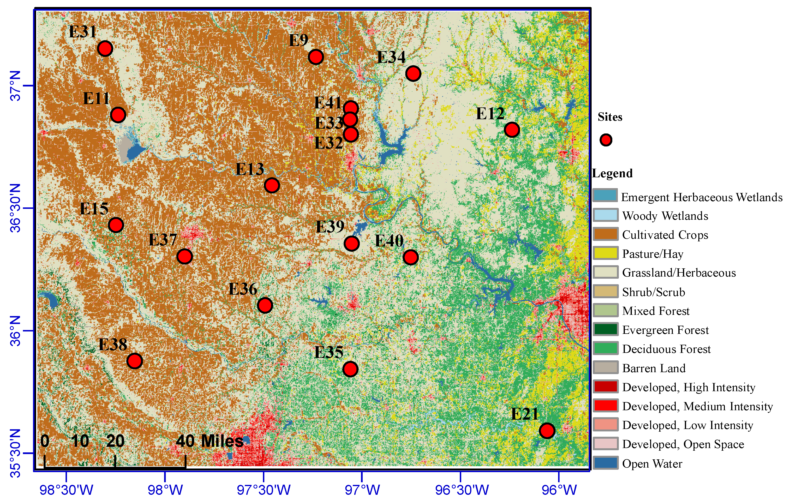
2.1. In-situ SM Measuremets

The assessments and comparisons were carried out over an area in the U.S. SGP shown in Figure 1. This region covers the southern part of Kansas and the northern part of Oklahoma with an area of nearly 90,000 km². The SGP observatory is part of the United States Department of Energy’s Atmospheric Radiation Measurement (ARM) networks, which consists of in-situ and remote-sensing instrument clusters and offers high-quality meteorological data and fluxes of water, energy and carbon [22]. The sites corresponding to the red dots in Figure 1 were equipped with soil temperature and moisture profile system (STAMP) deployed in early 2016. The STAMP system observes vertical profiles of soil temperature and water content at 5, 10, 20, 50 and 100 cm. The STAMP uses the Hydraprobe to measure soil water content at half hourly intervals. There are three sensor profile groups located 1 m apart. We calculated the mean value of three groups at 5 cm depth. The instruments are well calibrated and the uncertainty is less than 3% within a 95% confidence interval. The data were reviewed by the site scientist team once per week. Some data quality flags are used to indicate bad or questionable data, including the missing or the value out of the range. The specific information about the instruments can be read in the STAMP handbook [23]. Every site also installs rain gauge to record the precipitation at one-minute interval. The in-situ data are available from http://adc.arm.gov/discovery/. We averaged the 5 cm half hour SM data and accumulated one-minute precipitation data to get daily values. The land cover type of these sites is primarily winter wheat and grassland/pasture [23,24]. The soil type is mainly sandy loam and silt loam [23]. The specific information about every site is shown in

Table 1. South Great Plains site names and mean surface soil moisture(m³/m³), mean precipitation(mm/d), soil texture and surface type. The ID given in column 2 corresponds to the red dots in Figure 1. The short name of soil texture means: SiCL: silt clay loam, CL: clay loam, L: loam, SiL: silt loam, SL: sandy loam. The last three column corresponds to the area proportion of three main land cover within coarse-scale grid cell.

Site	ID	Mean SM a	Precip b	Soil Texture	Surface Type	Grassland c	Cultivated Crop c	Forest c
Ashton	E9	0.249	2.211	L	Pasture	28%	66%
Anthony	E31	0.211	1.720	SiL	Pasture	66%	28%
Byron	E11	0.292	2.049	L	Pasture	41%	46%
Lamont	E13	0.238	2.457	SL	Pasture/Wheat	18%	77%
Maple city	E34	0.272	2.391	SiCL	Pasture	87%
Marshall	E36	0.212	1.983	SL	Pasture	67%	13%	11%
Medford	E32	0.257	2.025	SiCL	Pasture	25%	56%
Morrison	E39	0.260	2.111	SiL	Pasture/Wheat	78%	15%
Newkirk	E33	0.237	2.573	SiL	Pasture/Wheat	20%	73%
Okmulgee	E21	0.191	2.034	SiCL	Forest	14%		58%
Omega	E38	0.203	1.965	SiL	Pasture/Wheat	27%	68%
Pawhuska	E12	0.257	2.027	SL	Native Prairie	53%		37%
Pawnee	E40	0.304	3.650	SiL	Pasture	65%		20%
Peckham	E41	0.303	3.171	SiL	Pasture/Wheat	29%	58%
Ringwood	E15	0.083	1.706	SL	Pasture	38%	50%
Tryon	E35	0.30	2.127	CL	Pasture	54%		29%
Waukomis	E37	0.217	1.789	SiL	Pasture/Wheat	20%	72%

^a Daily mean SM of each site, ^b Daily precipitation of each site, ^c Grassland, cultivated crop and forest are three main land cover within coarse-scale grid cell, the rest land cover types are less than 10%.

. The SGP SM observation we used here is called a sparse network, which means that there is just one group of sensors located within a remote sensing or modeled grid cell. The period used for assessments and comparisons was chosen for all datasets available from January 2016 to December 2017. It should be noted that the representativeness of SM of each site also has an impact on the comparison analysis of three SM products (SMAP, ESACCI A and NLDAS-2). The representativeness errors have different definitions in different scenes. It is hard to analyze its impact on the assessment quantitatively. In this study, we just defined representativeness errors as the spatial deviations between point-scale in-situ measurements and grid coarse-scale SM products. According to some previous studies, the land cover patterns have a dominant impact on the representativeness of point-scale SM measurements at finer spatial scales (within a satellite footprint) [25], and therefore, we respectively compared the vegetation type of each site with the main vegetation type of the corresponding grid cell, which would be used to determine the representativeness of SM of each site. Based on the 2016 national land cover database 2016 (NLCD 2016), we determined the main land cover type of every satellite grid cell. The NLCD is based on the Multi-Resolution Land Characteristics (MRLC) with 16 land use classes and 30 m resolution [26]. We aggregated the 30 m pixel to the products SM data scale (10 km) and counted the proportion of main land cover area (the proportion is larger than 10%). The results are shown in the last three columns of Table 1.

2.2. SMAP L3

The SM satellite product used in this study is the passive enhanced level-3 product (L3SMPE), which is a daily composite of SMAP enhanced level-2 products (L2SMPE) that presents volumetric surface SM (0–5 cm, m³/m³). The NASA SMAP mission was launched on January 31st, 2015. The capability of the mission to measure SM relies on two instruments: a synthetic aperture radar and a radiometer operating at an L-band. The radar instrument had failed since July 7, 2015. The L-band brightness temperature is sensitive to SM and relatively insensitive to surface roughness and vegetation, which makes it the most suitable band to measure SM. The L2SMPE product is derived from the SMAP Enhanced L1 Gridded Brightness Temperature Product (L1CTB_E) (posted at a 9 km grid cell) based on the Backus-Gilbert optimal interpolation technique [27]. The L3SMPE product is a daily product generated by compositing L2SMPE, which has an intermediate resolution (~9 km) and revisits twice a day (ascending and descending). We chose the descending (6 AM local time) SM retrievals instead of the ascending (6 PM local time) data because surface soil and vegetation are in better thermal equilibrium conditions at 6:00 AM [28]. The SMAP products can be downloaded freely from the National Snow and Ice Data Center (NSIDC) (https://nsidc.org/data/SPL3SMP). The SMAP enhanced SM is retrieved from the interpolated SMAP brightness temperature observations at 9 km. This is because the SMAP radiometer sampling provides overlapping observations along the scan and along the track, which makes reconstructing the observed scene with improved resolution possible. More details about the SMAP enhanced passive SM product can be found in [29].

2.3. ESACCI

The ESACCI SM product merges multi-source active and passive microwave SM products that have different characteristics, which is a global daily, long-term SM record with a spatial resolution of 0.25° [30]. The ESACCI consists of three individual datasets, including the active, passive and the combined (active-passive) products. The active product is generated only by merging active microwave-based datasets (i.e., scatterometers (SCAT and ASACT), the passive product is generated only by merging passive microwave-based datasets (i.e., Scanning Multichannel Microwave Radiometer [SMMR], Special Sensor Microwave Imager [SSM/I], Tropical Rainfall Measuring Mission Microwave Imager [TMI], AMSR-E, WindSat, AMSR-2 and SMOS utilizing the LPRM) and the combined product is generated by merging both active microwave- and passive microwave-based datasets. The product we used here is the latest released ESACCI SM v04.4, which uses a new algorithm from previous versions, based on uncertainty analysis to combine active and passive microwave products from the previous versions. More detailed descriptions can be found in [31].

2.4. NLDAS-2

The NLDAS-2 is an offline modeling system, running four land surface models (CLM (Community Land Model), Noah, Mosaic and VIC) at a 0.125°resolution over the continental United States [32]. It should be noted that NLDAS precipitation data sets are primarily derived from daily National Oceanographic and Atmospheric Administration (NOAA) Climate Prediction Center (CPC) precipitation gauge data with an orographic adjustment using the Parameter-evaluation Regressions on Independent Slopes Model (PRISM) [33]. Hence, it is relatively reliable in the United States. We chose the Noah version. The Noah model is a land surface model developed by the National Centers for Environment Prediction (NCEP). The model has four soil layers with spatially invariant depths: 0–10, 10–40, 40–100 and 100–200 cm and simulates SM at the middle of each layer (5, 25, 70 and 150 cm) [32] The first layer was used in this study because it is the best match to the in-situ measurements and remotely sensed SM datasets. The temporal resolution of the dataset is hourly, so we average all values in a day to get the daily SM.

2.5. Evaluation Methods and Metrics

We first compared the difference between three coarse resolution SM products with respect to in-situ observations. All three types of datasets were initially converted to daily averages due to the different temporal resolutions. However, remotely sensed products had gaps in long-term continuous observations, thus, available samples of the three products were different. As expected, model-based SM products could be obtained during the entire study period. The advantages of ESACCI in this temporal coverage come from the fact that it was a combined product of multiple datasets. The SMAP product had the lowest temporal samples. We had two sample strategies to deal with the discrepancy in temporal interval. One was selecting the days when all three products and in-situ measurements had valid values to keep the sample numbers the same. The other was using every product that could coincide with in-situ measurements, respectively. We used the t-test to determine if there was a significant discrepancy between statistical metrics using different methods of sampling. The results implied that there was no difference in statistical results between the two sampling strategies.

It should be noted that a direct comparison between the spatial SM retrievals and the ground measurements (precipitation distribution, soil characteristics, topography and vegetation) is challenging due to the SM heterogeneity [25]. The discrepancy was evaluated according to four common metrics: (1) correlation coefficient (R), (2) bias, (3) root-mean-square difference (RMSD) and (4) unbiased root-mean-square difference (ubRMSD) [34]. For both SMAP and ESACCI data products, only those SM data whose retrieval quality fields indicated good retrieval quality were used in evaluation. An alternative is to use an average mean SM of multi-site observation, just like the CVS. However, in our case, every grid cell has just one observation. Some researchers used unbiased RMSD (ubRMSD) instead of RMSD in the analysis by subtracting the temporal mean bias. The degree of association between the in-situ reference data and product datasets was calculated using the Pearson correlation coefficient (R) according to Equations (1)–(4), where SM_re represents a satellite- or model-based SM retrieval (m³/m³) and SM_m means the in-situ measurement (m³/m³). N represents the total number of data pairs. Cov in Equation (1) represents the covariance of two datasets, the ${\sigma }_{rs} \mathrm{and} {\sigma }_m$ represent the variance of satellite and modeled data. Furthermore, to ensure statistical robustness, stations with at least 100 paired observations were used in this study:

$$\mathrm{R}=\frac{Cov\left(S{M}_{re},S{M}_m\right)}{{\sigma }_{re}{\sigma }_m}$$

(1)

$$\mathrm{RMSD}=\sqrt{\frac{1}{N}{{\displaystyle \sum }}_{i=1}^N{(S{M}_{re}-S{M}_m)}_i^2}$$

(2)

$$\mathrm{bias}=\frac{1}{N}{{\displaystyle \sum }}_{i=1}^N{(S{M}_{re}-S{M}_m)}_i^{}$$

(3)

$$\mathrm{ubRMSD}=\sqrt{RMS{D}^2-bia{s}^2}$$

(4)

The evaluation of SM products can vary significantly across different time scales [35]. Various SM products may represent a similar drying and wetting cycle but capture diverse short-term fluctuations. Therefore, besides comparing the raw times series of in-situ measurements with the modelled or remotely sensed products, we also want to use a moving-average window to decompose the raw timeseries into a low-frequency SM dynamic and a higher-frequency anomaly. As shown in Equation (5), the t means the SM value at day t obtained from remote sensing or in-situ measurements or modelled data, while [t − 17,t + 17] means a time window of 35 days (5-week) centered on day t [31,32]. The overbar means the average of the SM values of 35 days, referred as the seasonality. The short-term anomalies $S{M}_{ano}\left(t\right)$ are calculated by subtracting seasonality from the raw timeseries SM values. If the days of a particular time window that all SM datasets are available are less than 25%, the moving average should not be calculated:

$$S{M}_{ano}\left(t\right)=SM\left(t\right)-\overline{SM\left[t-17,t+17\right]}$$

(5)

3. Results

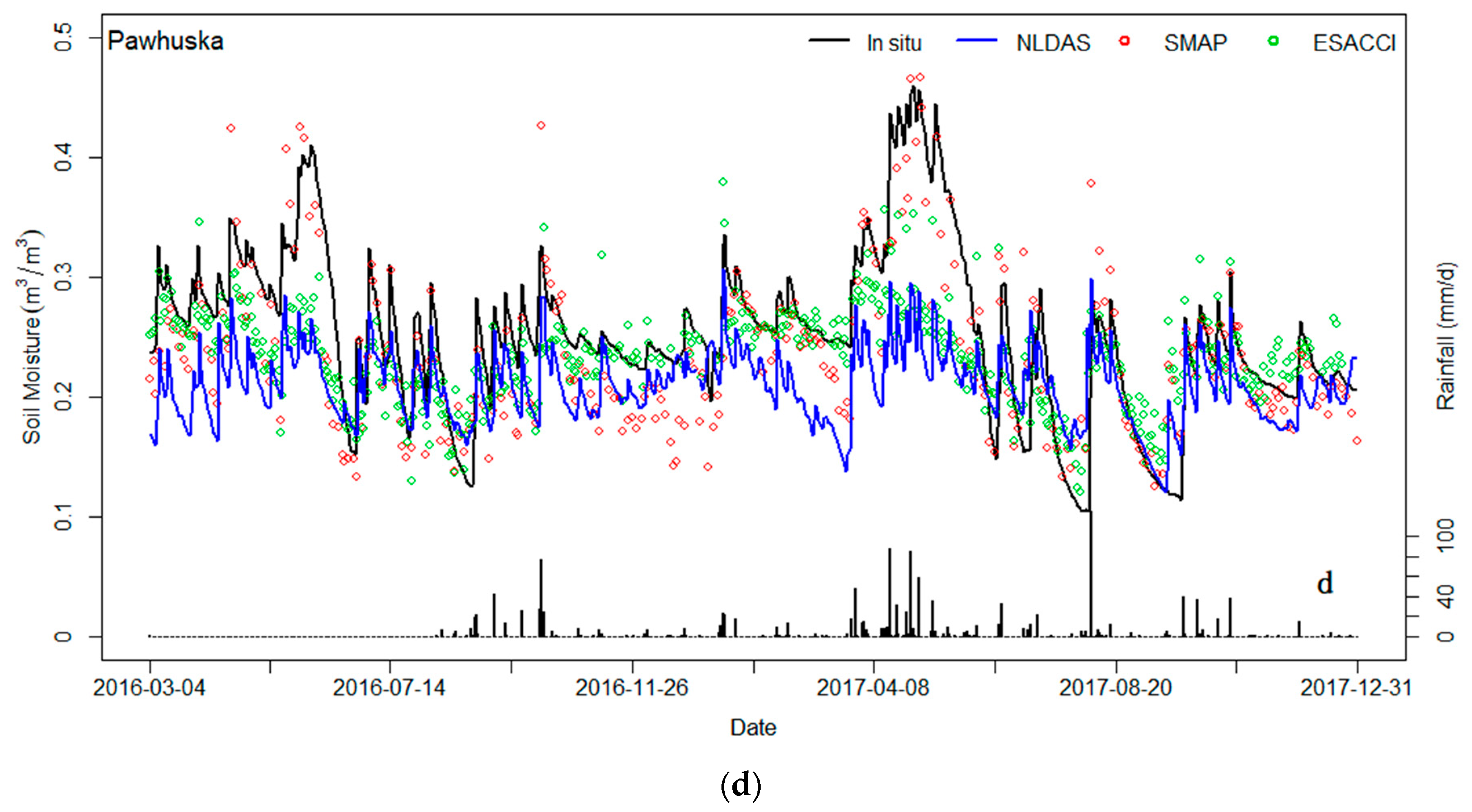
3.1. Temporal Evaluation with in-situ Observations

Table 2. Statistics of the comparison between SM products and in-situ observations. RMSD, ubRMSD and BIAS are the root mean square error (unit: m³/m³), the unbiased RMSD (unit: m³/m³) and the mean bias (unit: m³/m³), respectively. R is the temporal correlation. The network acronyms correspond to the first three letters of the site name. N means the available days that both three products and in-situ measurements have valid values.

Site	SMAP			ESACCI			NLDAS-2			N
	R	Bias	ubRMSD	R	Bias	ubRMSD	R	Bias	ubRMSD
Ash	0.87	0.018	0.054	0.62	0.036	0.058	0.79	0.061	0.055	266
Ant	0.76	−0.037	0.043	0.62	0.035	0.049	0.58	0.019	0.052	296
Byr	0.76	−0.078	0.052	0.54	−0.026	0.070	0.80	0.003	0.062	275
Lam	0.78	−0.003	0.054	0.55	0.037	0.060	0.69	0.056	0.058	266
Map	0.70	−0.008	0.059	0.58	0.014	0.063	0.53	0.04	0.066	259
Mar	0.83	0.003	0.042	0.68	0.052	0.056	0.81	0.028	0.049	290
Med	0.65	0.002	0.074	0.43	0.029	0.090	0.75	0.024	0.077	263
Mor	0.78	−0.026	0.050	0.66	0.007	0.064	0.73	0.007	0.060	251
New	0.80	0.029	0.052	0.46	0.052	0.079	0.82	0.065	0.067	263
Okm	0.70	0.058	0.051	0.62	0.099	0.057	0.74	0.086	0.052	247
Ome	0.80	−0.008	0.045	0.73	0.049	0.053	0.74	0.085	0.056	299
Pawh	0.82	−0.017	0.041	0.74	−0.022	0.051	0.72	−0.044	0.054	234
Pawn	0.79	−0.068	0.045	0.73	−0.035	0.051	0.72	−0.024	0.057	289
Pec	0.79	−0.055	0.050	0.50	−0.032	0.065	0.77	−0.018	0.055	271
Rin	0.65	0.078	0.043	0.62	0.062	0.032	0.59	0.067	0.034	270
Try	0.73	−0.079	0.052	0.61	−0.052	0.060	0.57	−0.053	0.064	249
Wau	0.81	−0.019	0.042	0.70	0.052	0.056	0.74	0.074	0.059	214

summarizes the statistical metrics for the comparison between SMAP L3 passive enhanced products (hereafter referred to as SMAP), ESACCI, NLDAS-2 and in-situ SM values. As for bias, there was no consistency among the three products. The SMAP presented a little dry bias in terms of the temporal mean, whereas the ESACCI and NLDAS-2 presented a wet bias (the median biases of three products were 0.008 m³/m³, 0.036 m³/m³ and 0.028 m³/m³, respectively). Regarding the R and ubRMSD, the SMAP products showed the highest R (median R is 0.79) and the lowest ubRMSD (median ubRMSD is 0.05), followed by the NLDAS-2 (median R: 0.74; median ubRMSD: 0.06) and the ESACCI (median R: 0.63; median ubRMSD: 0.06), as shown in Figure 2. In terms of the correlation coefficient, the SMAP outperformed ESACCI for all sites according to the results of the t-test (P < 0.05). However, at some sites (such as Byron and Medford), SMAP performed a little worse than NLDAS-2. In addition, there was no obvious low R value found in SMAP for all sites, whereas the R values between ESACCI, NLDAS-2 and in-situ measurements were poor at some sites (Maple city for NLDAS and Medford for ESACCI). The SMAP tended to underestimate SM in 11 sites (11/17), whereas the ESACCI and NLDAS-2 tended to overestimate SM in most sites (12/17, 13/17). As for ubRMSD, as shown in Figure 2a, the median value of SMAP was lower than that of other two products, though it exceeded the SMAP mission requirement (ubRMSD below 0.04 m³/m³). The median value of ESACCI was little lower than that of the NLDAS-2 in terms of ubRMSD. The variation of the ubRMSD of the ESACCI for all sites was larger than for the other two products. There was no direct connection between the R and ubRMSD for all sites. The distribution of R between two remotely sensed products was similar. For the Ringwood site, the three products had a relatively low R. The ESACCI and NLDAS-2 had the lowest values in terms of ubRMSD (0.032 m³/m³ and 0.034 m³/m³), which were smaller than that of the SMAP. Meanwhile, the Medford site was different from other sites because all three datasets exhibited the largest ubRMSD: 0.074, 0.090 and 0.077.

Figure 3 illustrates the time series behavior of the three SM products (SMAP, ESACCI and NLDAS-2) and permanent in-situ measurements. The daily precipitation data measured by the networks were also added to the figure as a bar plot. For some permanent observation sites, all three products show generally good agreement with in situ measurements. The SMAP product was shown to have a higher correlation coefficient than ESACCI and NLDAS, which is reflected in Figure 3. The remotely sensed or model-based data showed consistency with the precipitation events. After a precipitation event, high soil moisture values were estimated in both products. However, if the rain continued (April in 2017), the SMAP retrievals would be overestimated over the site measurement for some sites (Ashton, Medford), because the sensors measured 5-cm depth SM in soil, whereas the puddles after the rainfall would affect the satellite measurements. Due to the restriction of the SM saturation conditions, the modeled products would not overestimate the in-situ measurement too much. Following a dry period, both products showed low SM values, thus reflecting dry soil conditions. For the Ringwood site, the annual precipitation is low and the main soil texture is sandy, thus, the surface SM of this site was very low. It was revealed that all three products overestimated the SM with a large positive bias of 0.078, 0.062 and 0.067 m³/m³. When precipitation continued to occur in a period of time (usually in June or July), it would lead to an obvious overestimation of SM by SMAP and ESACCI.

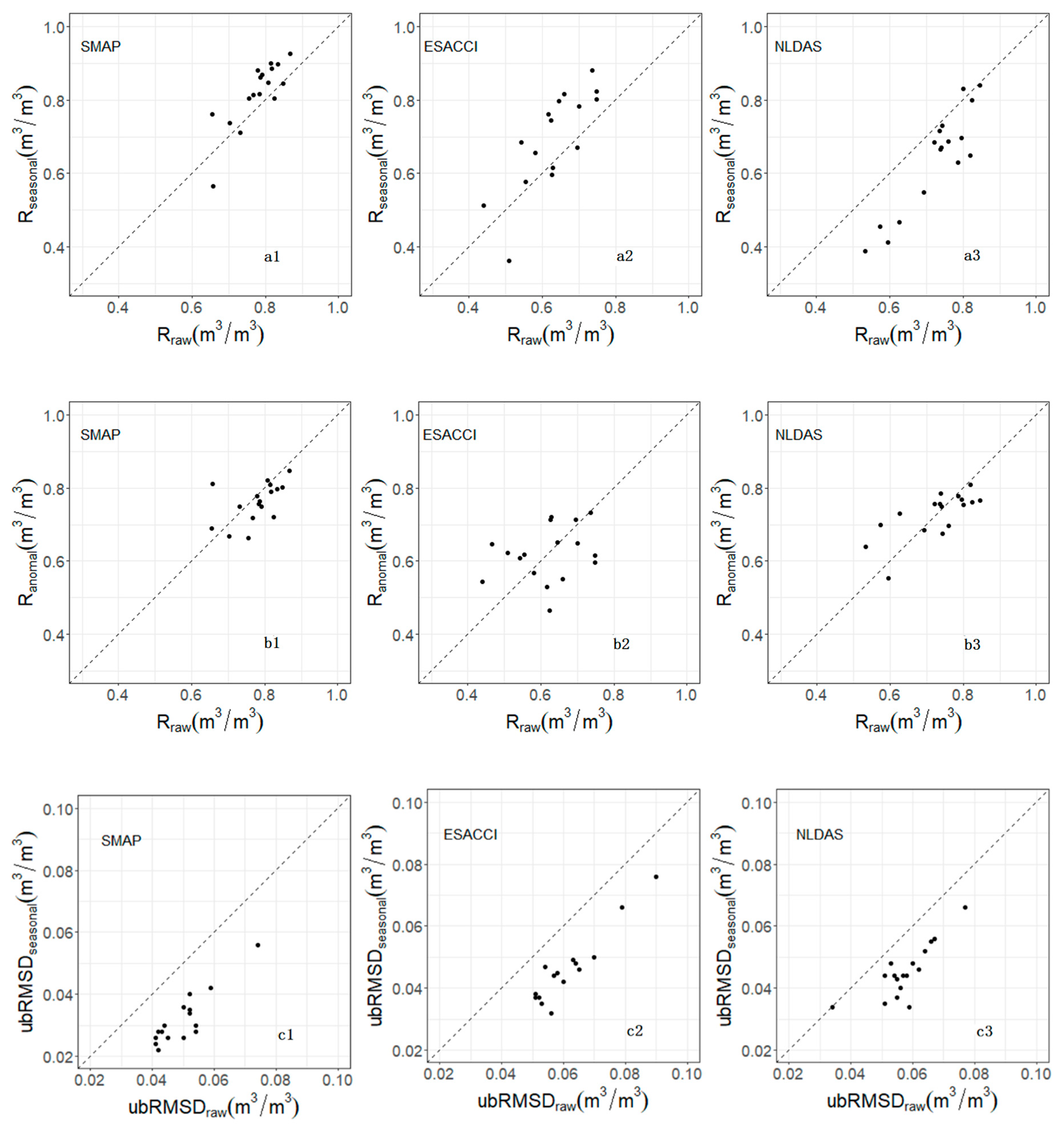
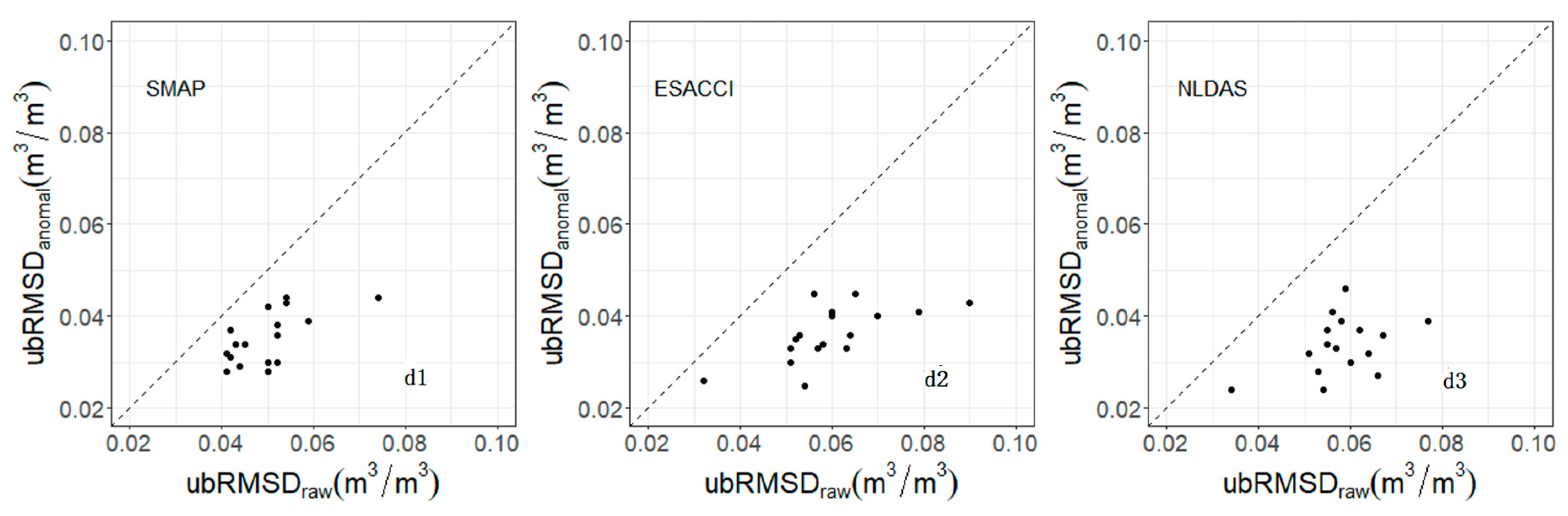
3.2. Comparison of Seasonal and Anomaly Components

The results presented above give an overview of the comparison of different products for all time periods. We decomposed the daily time series SM values into seasonal and anomaly components by using Equation (5). The ability of the product to capture the short-term SM variations was also considered as an accuracy metric of the datasets. For short-term seasonal and anomaly components, the temporal R between in-situ and satellite- or model-based products was inconsistent. As shown in the scatterplot in Figure 4 and

Table 3. Statistics of the comparison between SM products and in-situ observations in terms of anomaly R, Bias (m³/m³), ubRMSD (m³/m³), u. N means the available days that both three products and in-situ measurements have valid values.

Site	SMAP L3			ESACCI			NLDAS-2			N
	R	Bias	ubRMSD	R	Bias	ubRMSD	R	Bias	ubRMSD
Ash	0.848	0.000	0.044	0.714	−0.002	0.034	0.769	−0.001	0.034	266
Ant	0.779	0.000	0.028	0.65	−0.002	0.033	0.729	−0.001	0.028	267
Byr	0.718	−0.002	0.036	0.607	−0.003	0.04	0.753	0.002	0.037	309
Lam	0.756	0.000	0.043	0.617	−0.002	0.041	0.685	−0.002	0.039	266
Map	0.667	−0.001	0.039	0.567	−0.001	0.04	0.699	−0.001	0.027	259
Mar	0.796	−0.002	0.031	0.714	−0.002	0.033	0.767	−0.001	0.032	272
Med	0.69	−0.001	0.044	0.543	−0.002	0.043	0.696	−0.001	0.039	263
Mor	0.764	0.000	0.03	0.55	0.000	0.036	0.757	0.001	0.03	251
New	0.82	0.000	0.038	0.647	−0.001	0.041	0.81	−0.001	0.036	263
Okm	0.662	0.001	0.028	0.465	0.000	0.025	0.675	0.001	0.019	242
Ome	0.809	−0.002	0.045	0.732	0.049	0.053	0.745	0.085	0.056	299
Paw	0.721	0.000	0.032	0.596	−0.001	0.03	0.756	−0.001	0.024	234
Pawn	0.802	−0.001	0.029	0.616	−0.001	0.035	0.786	−0.001	0.033	255
Pec	0.75	−0.001	0.042	0.623	−0.002	0.045	0.777	−0.001	0.041	263
Rin	0.812	0.000	0.034	0.72	−0.002	0.026	0.552	−0.003	0.024	270
Try	0.749	−0.001	0.03	0.529	−0.001	0.04	0.699	−0.001	0.032	249
Wau	0.789	−0.002	0.037	0.648	−0.003	0.045	0.752	−0.001	0.046	214

, for most sites (13/17), the temporal anomaly of the SMAP product showed a weaker correlation with in-situ data than the raw time series. Meanwhile, the same trend of ESACCI and NLDAS-2 was shown for fewer sites (8/17, 10/17). In contrast, the temporal seasonality indicated that remotely sensed data were more effective at detecting interannual and seasonal patterns than single precipitation events. As shown in Figure 4, for most sites (13/17), the R of the seasonality component of SMAP improved compared with the original time series, as well as the ESACCI (12/17). However, for NLDAS-2, the seasonal R between in-situ measurements decreased compared with the original. The potential cause of the lower correlation values may be related to the vegetation type. The vegetation dynamic interpretation of the model simulation was based on leaf area index (LAI) for different sites, the vegetable types were mainly grassland and pasture, and they had different growing periods. Locally observed rainfall (the main driver of SM temporal pattern) could introduce discrepancies when compared to coarse resolution products. Moreover, the model-based data performed better for anomaly time series, and they had a relative higher R compared with in-situ measurements and a smaller ubRMSD than the remotely sensed data. The high accuracy of input precipitation data might account for this.

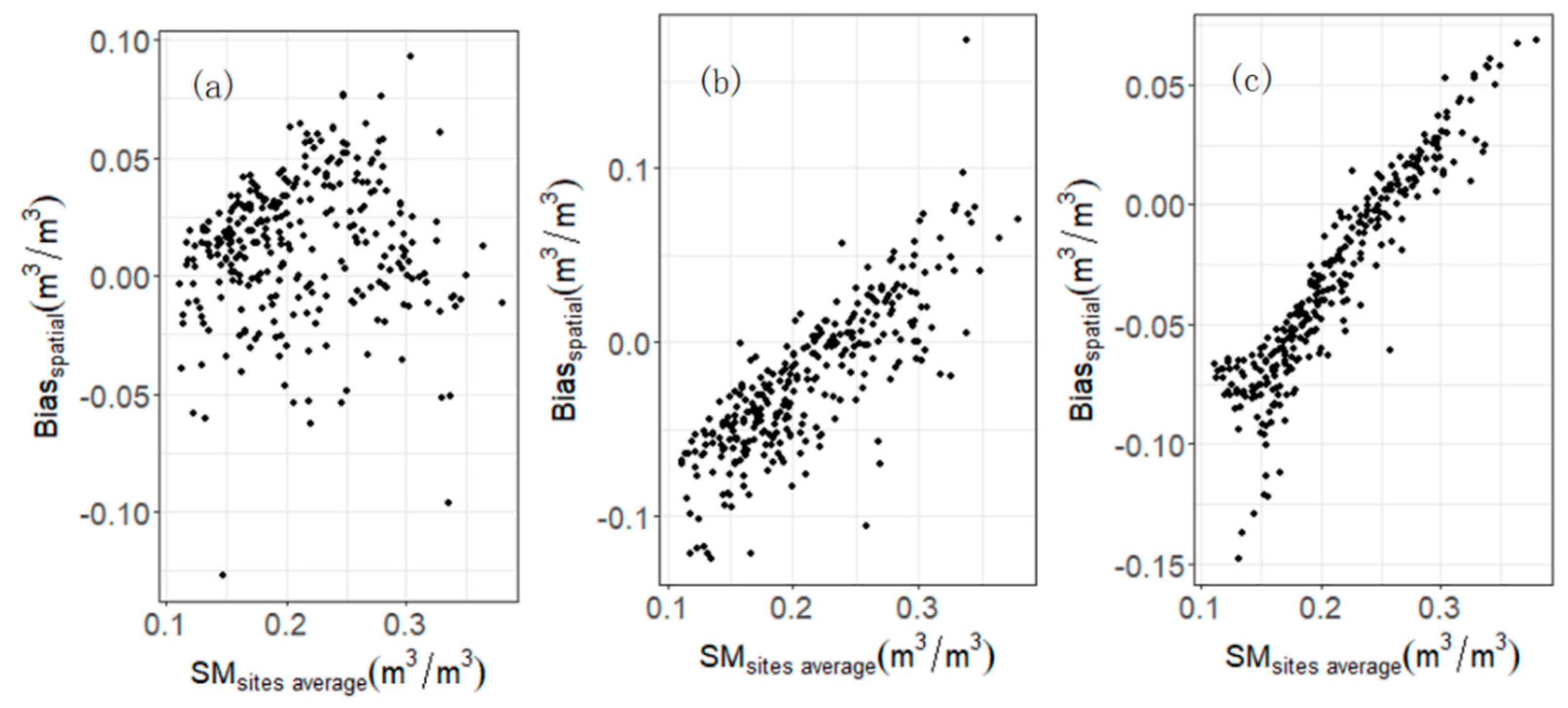
3.3. Spatial Analysis with in-situ Observations

Although the dense networks provide reliable satellite footprint scale SM values, they just focus on temporal dynamics at one grid cell. It is critical to evaluate whether various SM products actually represent real SM spatial patterns. All permanent observation sites used in this study were located in different grid cells. For these sites, spatial analysis was performed to estimate the agreement in spatial patterns of in-situ SM with three SM products. We calculated the daily spatial R, bias and ubRMSD with ground-based observations. The Figure 5 shows the time series plot of daily R and bias. The lowest of Figure 5 depicts the temporal evolution of spatial mean SM of this region, which is calculated by averaging all 17 sites observations. Not all sites had corresponding valid satellite retrievals in one day; when the valid retrievals were less than six, the result of this day was discarded.

As shown in Figure 5, the spatial R between three products and in-situ measurements had a wider range of variation than the temporal R. In some days corresponding to low SM values, all three products data had poor values in spatial R. The spatial bias of three products might be related to the region average SM values of the day. The SM values showed a continuous decreasing trend in the autumn of 2016, while the spatial bias also followed the trend, especially for the modelling data. Therefore, we drew scatter plots (Figure 6) about the spatial variations of three products (bias) and the average SM values. The relationship between the three products and in-situ measurements were inconsistent in terms of the spatial R and bias. For ESACCI and NLDAS, the products overestimated the in-situ measurements in low SM values, which was also reflected in Figure 3. A strong linear increasing trend was observed between the average SM value and the bias. For SMAP, the spatial bias did not have an obvious connection with the spatial mean SM. One possible explanation for that is that high SM usually corresponds to the days during or after precipitation; for the modeled data, precipitation was the main reason for the bias between the in-situ and retrievals, and modeled data overestimated the in-situ measurements at high SM and overestimated the in-situ measurements at low SM. In contrast, for the SMAP, remotely sensed data had no such pattern. This indicates that the error source from remotely sensed and modeled data were quite different.

4. Discussion

4.1. Similarities and Differences with Other Validation Results

It is critical to assess the reliability of SM products before using them. By comparing multiple sources of SM datasets, we can obtain knowledge of the strengths and weaknesses of different products. There are two ways to evaluate remotely sensed data. One is to compare with the in-situ measurements [20], and the other is to compare with the modeling data [36]. Compared with other validation results, there are some similarities and differences. The SMAP product validation was based on a set of core validation sites (CVS) [28]. The CVSs provided high-quality in-situ SM measurements and used an up-scaled method to acquire quasi-spatial SM reference data through observations at multiple locations. The validation obtained from the CVSs was better than that obtained through other conventional SM networks. The ubRMSD of most CVSs was less than 0.04 m³/m³, which met the target of the SMAP mission [28]. According to previous studies, the SMAP generally captures the dynamic range of SM better than other satellite products in terms of having a higher R and a lower ubRMSD [17,19,37,38]. The ESACCI, which is a combined product merging multiple remotely sensed data sources, except the SMAP, has an advantage of long-term climate data records and increase the sampling time intervals. Moreover, the combined ESACCI may perform better than individual products in some regions [18,30]. Although the statistical results of individual site were inconsistent, The results indicate that the SMAP outperforms the ESACCI with higher temporal R (SMAP:0.65–0.87; ESACCI:0.43–0.74) and lower ubRMSD (SMAP:0.041–0.074m³/ m³; ESACCI:0.032–0.09 m³/ m³) with respect to in-situ measurements. Therefore, the next generation of ESACCI may consider including the SMAP in the synthetizes. Model simulation is used as a benchmark for remotely sensed data, especially in some regions, such as the US or Europe; the accuracy of precipitation data is high, and model-based SM can capture the temporal change well. However, in some areas where the accuracy of meteorological data cannot be guaranteed, satellite products are proven to be better than model simulations [36,39]. In this study, though the precipitation data of the NLDAS-2 are similar to the site’s measurement and the model-based data and the NLDAS captured the seasonal and anomaly time series well, the SMAP also had a high R value compared with the in-situ data in terms of seasonality and anomaly. This indicates that remotely sensed SM data can reflect the change of SM due to short-term precipitation events. In addition, the SMAP captures the drying process better than the model-based data and has less difference compared with the in-situ data. All of these show the promising potential of remotely sensed data for drought monitoring and rainfall estimation [40,41].

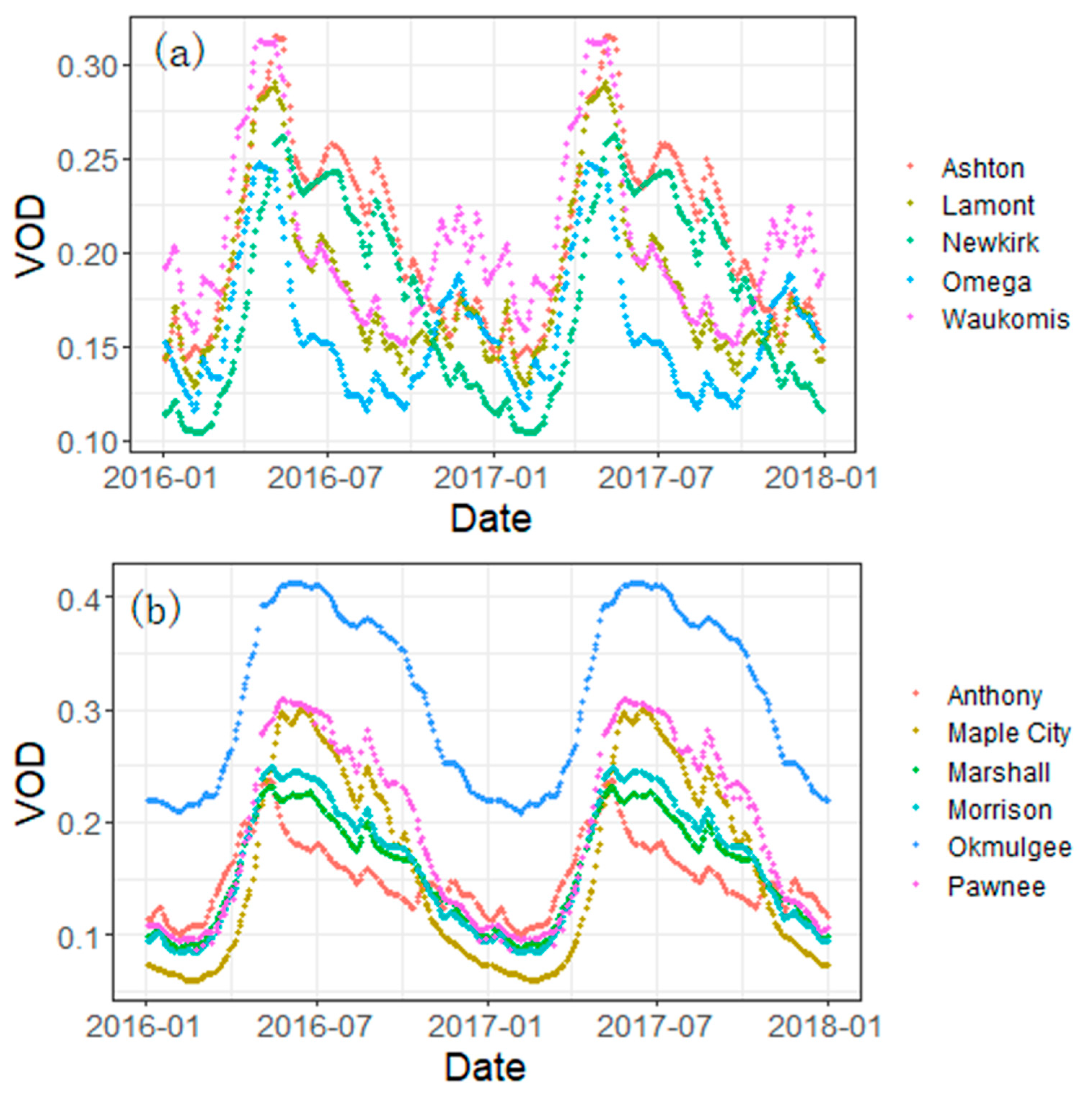
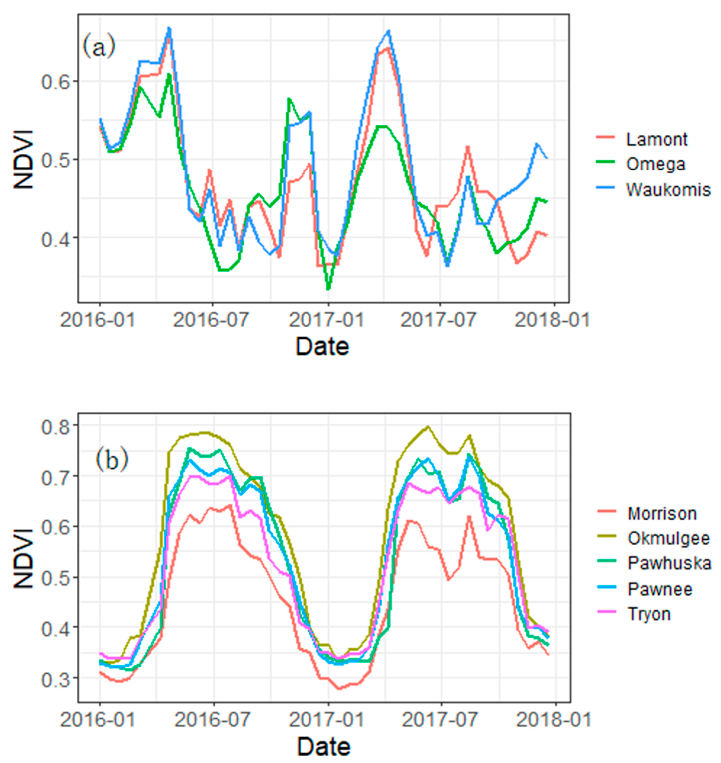
4.2. Analysis of the Possible Reasons for the Discrepancy between Different Products

Another important purpose of this study is to analyze the possible reasons for the discrepancy between the remotely sensed and modeling products. First, the accuracy of sensors used in ground measurement also affects the performance of satellite and modeling products compared with in-situ products. According to the instrument handbook [22], the sensors were well calibrated and the uncertainty of SM measurement is within 3% of the measured values, which was far less than the difference between three products and ground-based observations In addition, various satellite products might have different infiltrate depth, depending on the soil texture and SM content [42,43]. For SMAP, the uncertainty caused by the depths was estimated as a range (0–5 cm) with a set of uncertainties, not a certain depth [29]. The ESACCI is a combined product for which active and passive products have different sensing depths, but they are all defined as “surface soil moisture” and are around 5 cm [30]. The NLDAS output 5 cm as the average SM of the first layer, which is not equal to the true 5 cm ground measured depth. The mis-match of retrieved depth were usually considered to be systematic errors, which were less connected to the temporal R and ubRMSD [44]. For ESACCI, satellite products to be combined were firstly scaled against GLDAS Noah (Global version of NLDAS) to harmonies their climatology [31]. Therefore, ESACCI and NLDAS estimates showed a similar wet bias during the drying period based on our results. We compared the temporal mean of 5 cm and 10 cm in-situ SM measurements as a reference. Indeed, the mean SM of 10 cm was wetter than the 5 cm data, but it was still drier than the ESACCI and NLDAS data. Besides the depth, there are other reasons for this deviation, which need further study.

According to our results, the spatial bias between the ground reference data and the three products is correlated with the SM values, especially for the modeling data. The uncertainty of precipitation data may account for that. After a rainfall event, the surface soil becomes wetter and the variation of spatial distribution increases, which is shown in Figure 5c. Data from all three products are lower than the in-situ data. With the soil drying, the remotely sensed data decrease accordingly; moreover, the modeling data show a slow drying rate, meaning the data will be wetter than the in-situ data. Thus, the bias between modeling data and in-situ observations is strongly dependent on the changing of the SM, whereas the remotely sensed data show less correlation with the reference SM values.

Another key issue regarding differences between the SM products is the mismatch of vegetation data between remotely sensed and modeling products, which also reflect whether the site is representative. As shown in Table 1, most sites can stand for the vegetation type of their pixel, except for Anthony, Medford. The vegetation around the site were often mixed with pasture and cultivated crop, whereas the grid cells were more dominated by one type. For example, the Lamont site is covered by wheat crop and pasture; however, the corresponding footprint pixel were most covered by the cultivated crop. Which would If alleviate the disparity between different scales. Our results indicate that systematic differences exist in remotely sensed or modeled products and ground measurements, even though the temporal dynamics are every similar. After conducting a moving mean calculation of 35 days, we found that the systemic bias mainly lay in the seasonal part. The anomaly ubRMSD decreased, whereas the anomaly R did not have a significant change.

There is further potential for improvement in SMAP SM retrievals. The improvements include use of better ancillary data (optimized vegetation water content (VWC] and better soil texture data). The vegetation canopy exerts significant effects on the soil-emitted energy [45]. Vegetation not only attenuates signals from soil surfaces but also emits radiation itself, leading to a reduced sensitivity of brightness temperature to SM. Accordingly, the influence of vegetation must be corrected accurately before achieving reliable SM estimations. Commonly, the effects of vegetation are mainly represented by the vegetation optical depth (VOD), which characterizes the radiation attenuation caused by vegetation The VOD of SMAP is estimated from the VWC, which is calculated by using a 10-year MODIS NDVI climatology data at 1-km spatial resolution. An empirical polynomial is established to calculate VWC from NDVI. Seasonal biases of remotely sensed or modeled SM products showed that most in-situ data that include managed agriculture exhibit significant time-dependent seasonal bias. According to a previous study, the performance of satellite products is worse for sites that are dominated by cultivated crop [28]. In general, the main vegetation type of the SGP region is cultivated crop and grassland/pasture; one site is covered by forest (Waukomis). We aggregated a 30 m land-cover map to the 9 km scale pixel and counted the crop, grassland and forest class of grid cells; we found that the main vegetation type of the footprint pixel was nearly consistent with the corresponding site. As shown in Figure 7, climatology vegetation optical depth (VOD) cannot indicate the discrepancy between the crop and grassland in terms of the growing period. The time variation of NDVI for winter wheat differed markedly from that of natural grassland, especially in summer. The winter wheat usually matured in late April [24]. After harvesting, the ground would be uncovered for a period of time, whereas the nature pasture continued growing. As shown in Figure 8, t crops the NDVI reached a maximum of about 0.6 in terms of NDVI. After harvest, the NDVI decreased sharply and maintained a relatively low value in the summer. In contrast, the NDVI of natural grassland increased consistently after entering the growth of vegetation and held a high value of about 0.7 in the summer. It was noted that the NDVI of pasture might vary irregularly due to cattle grazing or regular mowing. Besides the water stored in vegetation foliage, the intercepted precipitation or dew also had an effect on microwave radiation. Whether the free water in the canopy affected the microwave emission depended on the type and physical structure of vegetation [46], which would need to be considered in future research.

5. Conclusions

Assessing the discrepancy between the remotely sensed and modeling SM products is crucial for their utilization in scientific studies and applications and also improves our knowledge of how they can be further improved. This paper provides a comparison among SMAP, ESACCI and NLDAS-2 SM retrievals using 17 permanent in-situ measurements as ground reference over the SGP. The vegetation types of SGP are mainly wheat and pasture, which have different growing periods. The possible reasons behind the difference between remotely sensed or modeled products are also investigated and discussed in detail. The results demonstrate that (1) the temporal variation of the SMAP is more consistent with ground measurements, with a higher temporal correlation coefficient (median R = 0.78) than ESACCI (R = 0.62) and NLDAS-2 (R = 0.72). However, there is no significant discrepancy between the three products in terms of the ubRMSD, for which all values exceed the target (0.04 m³/m³). However, compared with other studies with respect to sparse networks, the metrics in this study had a relatively high accuracy. (2) After decomposing the original values into the seasonal and anomaly components, the seasonality part of remotely sensed data had even higher R than the model simulation, which indicates that the vegetation had an important impact on the seasonal change of SM, and remotely sensed data can capture that. There was no significant difference for correlation R between the anomaly satellite- or model-based datasets and in-situ measurements, which implies that the remotely sensed products have the potential to capture the short-term variation caused by a single rainfall event, like modeling products. (3) The distribution pattern of spatial metrics is different between the three products. For NLDAS and ESACCI, the bias was more related to the daily SM values. For SMAP, the bias was more random. In general, the SMAP is superior to the other two products, especially when the SM is at a low value. The remotely sensed products have the ability to reflect the occurrence of precipitation events. By comparing remotely sensed data and model simulations, we can see the potential advantages of combining two of them.

References

1. Koster, R.D. Regions of Strong Coupling Between Soil Moisture and Precipitation. Science 2004, 305, 1138–1140. [Google Scholar] [CrossRef] [Green Version]
2. Seneviratne, S.I.; Corti, T.; Davin, E.L.; Hirschi, M.; Jaeger, E.B.; Lehner, I.; Orlowsky, B.; Teuling, A.J. Investigating soil moisture–climate interactions in a changing climate: A review. Earth Sci. Rev. 2010, 99, 125–161. [Google Scholar] [CrossRef]
3. Corradini, C. Soil moisture in the development of hydrological processes and its determination at different spatial scales. J. Hydrol. 2014, 516, 1–5. [Google Scholar] [CrossRef]
4. Brocca, L.; Tarpanelli, A.; Filippucci, P.; Dorigo, W.; Zaussinger, F.; Gruber, A.; Fernández-Prieto, D. How much water is used for irrigation? A new approach exploiting coarse resolution satellite soil moisture products. Int. J. Appl. Earth Obs. Geoinf. 2018, 73, 752–766. [Google Scholar] [CrossRef]
5. Crow, W.T.; Ryu, D. A new data assimilation approach for improving runoff prediction using remotely-sensed soil moisture retrievals. Hydrol. Earth Syst. Sci. 2009, 13, 1–16. [Google Scholar] [CrossRef] [Green Version]
6. Jung, M.; Reichstein, M.; Schwalm, C.R.; Huntingford, C.; Sitch, S.; Ahlström, A.; Arneth, A.; Camps-Valls, G.; Ciais, P.; Friedlingstein, P.; et al. Compensatory water effects link yearly global land CO2 sink changes to temperature. Nature 2017, 541, 516–520. [Google Scholar] [CrossRef] [Green Version]
7. Brocca, L.; Ciabatta, L.; Massari, C.; Camici, S.; Tarpanelli, A. Soil Moisture for Hydrological Applications: Open Questions and New Opportunities. Water 2017, 9, 140. [Google Scholar] [CrossRef]
8. Wagner, W.; Hahn, S.; Kidd, R.; Melzer, T.; Bartalis, Z.; Hasenauer, S.; Figa-Saldaña, J.; De Rosnay, P.; Jann, A.; Schneider, S.; et al. The ASCAT soil moisture product: A review of its specifications, validation results, and emerging applications. Meteorol. Z. 2013, 22, 5–33. [Google Scholar] [CrossRef] [Green Version]
9. Njoku, E.G.; Jackson, T.J.; Lakshmi, V.; Chan, T.K.; Nghiem, S.V. Soil moisture retrieval from AMSR-E. IEEE Trans. Geosci. Remote Sens. 2003, 41, 215–229. [Google Scholar] [CrossRef]
10. Imaoka, K.; Maeda, T.; Kachi, M.; Kasahara, M.; Ito, N.; Nakagawa, K. Status of AMSR2 instrument on GCOM-W1. Proc. SPIE 2012, 8528, 852815. [Google Scholar]
11. Kerr, Y.H.; Waldteufel, P.; Wigneron, J.P.; Delwart, S.; Cabot, F.; Boutin, J.; Escorihuela, M.J.; Font, J.; Reul, N.; Gruhier, C.; et al. The SMOS mission: New tool for monitoring key elements of the global water cycle. Proc. IEEE 2010, 98, 666–687. [Google Scholar] [CrossRef] [Green Version]
12. Entekhabi, D.; Njoku, E.G.; O’Neill, P.E.; Kellogg, K.H.; Crow, W.T.; Edelstein, W.N.; Entin, J.K.; Goodman, S.D.; Jackson, T.J.; Johnson, J.; et al. The soil moisture active passive (SMAP) mission. Proc. IEEE 2010, 98, 704–716. [Google Scholar] [CrossRef]
13. Wigneron, J.P.; Jackson, T.J.; O’neill, P.; De Lannoy, G.; De Rosnay, P.; Walker, J.P.; Ferrazzoli, P.; Mironov, V.; Bircher, S.; Grant, J.P.; et al. Modelling the passive microwave signature from land surfaces: A review of recent results and application to the L-band SMOS&SMAP soil moisture retrieval algorithms. Remote Sens. Environ. 2017, 192, 238–262. [Google Scholar]
14. Dorigo, W.; Wagner, W.; Albergel, C.; Albrecht, F.; Balsamo, G.; Brocca, L.; Chung, D.; Ertl, M.; Forkel, M.; Gruber, A.; et al. ESA CCI Soil Moisture for improved Earth system understanding: State-of-the art and future directions. Remote Sens. Environ. 2017, 203, 185–215. [Google Scholar] [CrossRef]
15. Chen, Q.; Zeng, J.; Cui, C.; Li, Z.; Chen, K.-S.; Bai, X.; Xu, J. Soil Moisture Retrieval From SMAP: A Validation and Error Analysis Study Using Ground-Based Observations Over the Little Washita Watershed. IEEE Trans. Geosci. Remote Sens. 2018, 56, 1394–1408. [Google Scholar] [CrossRef]
16. Colliander, A.; Jackson, T.J.; Chan, S.K.; O’Neill, P.; Bindlish, R.; Cosh, M.H.; Caldwell, T.; Walker, J.P.; Berg, A.; McNairn, H.; et al. An assessment of the differences between spatial resolution and grid size for the SMAP enhanced soil moisture product over homogeneous sites. Remote Sens. Environ. 2018, 207, 65–70. [Google Scholar] [CrossRef]
17. Cui, C.; Xu, J.; Zeng, J.; Chen, K.S.; Bai, X.; Lu, H.; Chen, Q.; Zhao, T. Soil moisture mapping from satellites: An intercomparison of SMAP, SMOS, FY3B, AMSR2, and ESA CCI over two dense network regions at different spatial scales. Remote Sens. 2018, 10, 33. [Google Scholar] [CrossRef] [Green Version]
18. González-Zamora, Á.; Sánchez, N.; Pablos, M.; Martínez-Fernández, J. CCI soil moisture assessment with SMOS soil moisture and in situ data under different environmental conditions and spatial scales in Spain. Remote Sens. Environ. 2019, 225, 469–482. [Google Scholar] [CrossRef]
19. Ma, H.; Zeng, J.; Chen, N.; Zhang, X.; Cosh, M.H.; Wang, W. Satellite surface soil moisture from SMAP, SMOS, AMSR2 and ESA CCI: A comprehensive assessment using global ground-based observations. Remote Sens. Environ. 2019, 231, 111215. [Google Scholar] [CrossRef]
20. Zhang, R.; Kim, S.; Sharma, A. A comprehensive validation of the SMAP Enhanced Level-3 Soil Moisture product using ground measurements over varied climates and landscapes. Remote Sens. Environ. 2019, 223, 82–94. [Google Scholar] [CrossRef]
21. Chen, F.; Crow, W.T.; Colliander, A.; Cosh, M.H.; Jackson, T.J.; Bindlish, R.; Reichle, R.H.; Chan, S.K.; Bosch, D.D.; Starks, P.J.; et al. Application of Triple Collocation in Ground-Based Validation of Soil Moisture Active/Passive (SMAP) Level 2 Data Products. IEEE J. Sel. Top. Appl. Earth Obs. Remote Sens. 2017, 10, 489–502. [Google Scholar] [CrossRef]
22. Sisterson, D.L.; Peppler, R.A.; Cress, T.S.; Lamb, P.J.; Turner, D.D. The ARM Southern Great Plains (SGP) Site. Meteorol. Monogr. 2016, 57, 6.1–6.14. [Google Scholar] [CrossRef]
23. Cook, D.R. Soil Temperature and Moisture Profile (STAMP) System Instrument Handbook; DOE/SC-ARM-TR-186; Stafford, R., Ed.; DOE ARM Climate Research Facility: Argonne, IL, USA, 2018. [Google Scholar]
24. Bagley, J.E.; Kueppers, L.M.; Billesbach, D.P.; Williams, I.N.; Biraud, S.C.; Torn, M.S. The influence of land cover on surface energy partitioning and evaporative fraction regimes in the U.S. Southern Great Plains: Influence of Land Cover in U.S. SGP. J. Geophys. Res. Atmos. 2017, 122, 5793–5807. [Google Scholar] [CrossRef] [Green Version]
25. Crow, W.T.; Berg, A.A.; Cosh, M.H.; Loew, A.; Mohanty, B.P.; Panciera, R.; de Rosnay, P.; Ryu, D.; Walker, J.P. Upscaling sparse ground-based soil moisture observations for the validation of coarse-resolution satellite soil moisture products: UPSCALING SOIL MOISTURE. Rev. Geophys. 2012, 50. [Google Scholar] [CrossRef] [Green Version]
26. Danielson, P.; Yang, L.; Jin, S.; Homer, C.; Napton, D. An Assessment of the Cultivated Cropland Class of NLCD 2006 Using a Multi-Source and Multi-Criteria Approach. Remote Sens. 2016, 8, 101. [Google Scholar] [CrossRef] [Green Version]
27. Chaubell, J.; Chan, S.; Dunbar, R.; Entekhabi, D.; Peng, J.; Piepmeier, J.; Yueh, S. Backus-Gilbert optimal interpoaltion applied to enhance smap data: Implementation and assessment. In Proceedings of the 2017 IEEE International Geoscience and Remote Sensing Symposium (IGARSS), Fort Worth, TX, USA, 23–28 July 2017; pp. 2531–2534. [Google Scholar] [CrossRef]
28. Colliander, A.; Jackson, T.J.; Bindlish, R.; Chan, S.; Das, N.; Kim, S.B.; Cosh, M.H.; Dunbar, R.S.; Dang, L.; Pashaian, L.; et al. Validation of SMAP surface soil moisture products with core validation sites. Remote Sens. Environ. 2017, 191, 215–231. [Google Scholar] [CrossRef]
29. O’Neill, P.E.; Chan, S.; Njoku, E.; Jackson, T.J.; Bindlish, R. Algorithm Theoretical Basis Document (ATBD): L2/3_SM_P; National Aeronautics and Space Administration: Washington, CA, USA, 2015. [Google Scholar]
30. Dorigo, W.A.; Gruber, A.; De Jeu, R.A.M.; Wagner, W.; Stacke, T.; Loew, A.; Albergel, C.; Brocca, L.; Chung, D.; Parinussa, R.M.; et al. Evaluation of the ESA CCI soil moisture product using ground-based observations. Remote Sens. Environ. 2015, 162, 380–395. [Google Scholar] [CrossRef]
31. Gruber, A.; Scanlon, T. Evolution of the ESA CCI Soil Moisture climate data records and their underlying merging methodology. Earth Syst. Sci. Data 2019, 23, 1–37. [Google Scholar] [CrossRef] [Green Version]
32. Xia, Y.; Ek, M.B.; Wu, Y.; Ford, T.; Quiring, S.M. Comparison of NLDAS-2 Simulated and NASMD Observed Daily Soil Moisture. Part I: Comparison and Analysis. J. Hydrometeorol. 2015, 16, 1962–1980. [Google Scholar] [CrossRef]
33. Daly, C.; Neilson, R.P.; Phillips, D.L. A statistical-topographic model for mapping climatological precipitation over mountainous terrain. J. Appl. Meteor. 1994, 33, 140–158. [Google Scholar] [CrossRef] [Green Version]
34. Entekhabi, D.; Reichle, R.H.; Koster, R.D.; Crow, W.T. Performance Metrics for Soil Moisture Retrievals and Application Requirements. J. Hydrometeorol. 2010, 11, 832–840. [Google Scholar] [CrossRef]
35. Molero, B.; Leroux, D.; Richaume, P.; Kerr, Y.; Merlin, O.; Cosh, M.; Bindlish, R. Multi-timescale analysis of the spatial representativeness of in situ soil moisture data within satellite footprints. J. Geophys. Res. Atmos. 2018, 123, 3–21. [Google Scholar] [CrossRef] [Green Version]
36. Holgate, C.M.; De Jeu, R.A.M.; van Dijk, A.I.J.M.; Liu, Y.Y.; Renzullo, L.J.; Vinodkumar; Dharssi, I.; Parinussa, R.M.; Van Der Schalie, R.; Gevaert, A.; et al. Comparison of remotely sensed and modelled soil moisture data sets across Australia. Remote Sens. Environ. 2016, 186, 479–500. [Google Scholar] [CrossRef]
37. Al-Yaari, A.; Wigneron, J.-P.; Kerr, Y.; Rodriguez-Fernandez, N.; O’Neill, P.E.; Jackson, T.J.; De Lannoy, G.J.M.; Al Bitar, A.; Mialon, A.; Richaume, P.; et al. Evaluating soil moisture retrievals from ESA’s SMOS and NASA’s SMAP brightness temperature datasets. Remote Sens. Environ. 2017, 193, 257–273. [Google Scholar] [CrossRef] [PubMed] [Green Version]
38. Al-Yaari, A.; Wigneron, J.-P.; Dorigo, W.; Colliander, A.; Pellarin, T.; Hahn, S.; Mialon, A.; Richaume, P.; Fernandez-Moran, R.; Fan, L.; et al. Assessment and inter-comparison of recently developed/reprocessed microwave satellite soil moisture products using ISMN ground-based measurements. Remote Sens. Environ. 2019, 224, 289–303. [Google Scholar] [CrossRef]
39. Cheng, M.; Zhong, L.; Ma, Y.; Zou, M.; Ge, N.; Wang, X.; Hu, Y. A Study on the Assessment of Multi-Source Satellite Soil Moisture Products and Reanalysis Data for the Tibetan Plateau. Remote Sens. 2019, 11, 1196. [Google Scholar] [CrossRef] [Green Version]
40. Ford, T.W.; Quiring, S.M. Comparison of Contemporary In Situ, Model, and Satellite Remote Sensing Soil Moisture With a Focus on Drought Monitoring. Water Resour. Res. 2019, 55, 1565–1582. [Google Scholar] [CrossRef]
41. Paredes-Trejo, F.; Barbosa, H.; Rossato Spatafora, L. Assessment of SM2RAIN-Derived and State-of-the-Art Satellite Rainfall Products over Northeastern Brazil. Remote Sens. 2018, 10, 1093. [Google Scholar] [CrossRef] [Green Version]
42. Escorihuela, M.J.; Chanzy, A.; Wigneron, J.P.; Kerr, Y.H. Effective soil moisture sampling depth of L-band radiometry: A case study. Remote Sens. Environ. 2010, 114, 995–1001. [Google Scholar] [CrossRef] [Green Version]
43. Kaihotsu, I.; Asanuma, J.; Aida, K.; Oyunbaatar, D. Evaluation of the AMSR2 L2 soil moisture product of JAXA on the Mongolian Plateau over seven years (2012–2018). SN Appl. Sci. 2019, 1. [Google Scholar] [CrossRef] [Green Version]
44. Gruber, A.; De Lannoy, G.; Albergel, C.; Al-Yaari, A.; Brocca, L.; Calvet, J.-C.; Colliander, A.; Cosh, M.; Crow, W.; Dorigo, W.; et al. Validation practices for satellite soil moisture retrievals: What are (the) errors? Remote Sens. Environ. 2020, 244, 111806. [Google Scholar] [CrossRef]
45. Liu, K.; Wang, S.; Li, X.; Li, Y.; Zhang, B.; Zhai, R. The assessment of different vegetation indices for spatial disaggregating of thermal imagery over the humid agricultural region. Int. J. Remote Sens. 2020, 41, 1907–1926. [Google Scholar] [CrossRef]
46. Hornbuckle, B.K.; England, A.W.; Anderson, M.C. The Effect of Intercepted Precipitation on the Microwave Emission of Maize at 1.4 GHz. IEEE Trans. Geosci. Remote Sens. 2007, 45, 1988–1995. [Google Scholar] [CrossRef]
Figure 1. Southern Great Plains (SGP) domain and locations of soil moisture measurement sites are marked in red dots and they are labelled according to Table 1.
Remotesensing 12 02030 g001
Figure 2. Boxplot of R, Bias, ubRMSD for SMAP (a), ESACCI (b) and NLDAS_2 (c) SM products (a1a3) considering the original values; (b1b3) considering the seasonal values; (c1c3) considering the anomaly values; the median, first and third quantiles and outlier ranges are indicated by the center bold black line, bottom and top of the boxes and whiskers.
Remotesensing 12 02030 g002
Figure 3. Time-series comparison of three SM products (SMAP, NLDAS and ESACCI) and in-situ measurements. ((a): Ashton; (b): Marshall; (c): Medford; (d): Pawhuska).
Remotesensing 12 02030 g003aRemotesensing 12 02030 g003b
Figure 4. Scatterplot of temporal R between raw times and seasonal components of three SM data (a1a3); temporal R between raw times and anomaly components (b1b3); ubRMSD between raw times and seasonal components (c1c3); ubRMSD between raw times and anomaly components (d1d3).
Remotesensing 12 02030 g004aRemotesensing 12 02030 g004b
Figure 5. Time-series plot of spatial R (a) and bias (b) between three products and in-situ measurements; red points stand for SMAP, green points stand for ESACCI, blue points stand for NLDAS. The lowest figure (c) shows the average SM observations of all 17 sites.
Remotesensing 12 02030 g005
Figure 6. Scatterplot of daily spatial bias between SMAP (a), ESACCI (b), NLDAS (c) retrievals and in-situ observations against the daily average SM value of all 17 sites.
Remotesensing 12 02030 g006
Figure 7. Time-series plot of VOD (vegetation optical depth) of two different vegetation types: crop (a) and pasture (b). As referred to in Table 1, some sites are covered by crop, while others covered by pasture.
Remotesensing 12 02030 g007
Figure 8. Time-series plot of NDVI of two different vegetation types: crop (a) and pasture (b). As referred to in Table 1, some sites are covered by crop, while others covered by pasture.
Remotesensing 12 02030 g008