Article

Positional Accuracy Assessment of Lidar Point Cloud from NAIP/3DEP Pilot Project

1
KBR, Contractor to U.S. Geological Survey (USGS) Earth Resources Observation and Science (EROS), Sioux Falls, SD 57198, USA
2
United Support Services (USS), Contractor to USGS EROS, Sioux Falls, SD 57198, USA
3
USGS EROS, Sioux Falls, SD 57198, USA
4
US Dept. of Agriculture (USDA) Natural Resources Conservation Service (NRCS), Fort Worth Federal Center, Fort Worth, TX 76028, USA
5
USGS National Unmanned Aircraft System Project Office, Lakewood, CO 80225, USA
*
Author to whom correspondence should be addressed.
Remote Sens. 2020, 12(12), 1974; https://doi.org/10.3390/rs12121974
Submission received: 12 May 2020 / Revised: 15 June 2020 / Accepted: 18 June 2020 / Published: 19 June 2020
(This article belongs to the Special Issue Environmental Monitoring and Mapping Using 3D Elevation Program Data)

Abstract

:
The Leica Geosystems CountryMapper hybrid system has the potential to collect data that satisfy the U.S. Geological Survey (USGS) National Geospatial Program (NGP) and 3D Elevation Program (3DEP) and the U.S. Department of Agriculture (USDA) National Agriculture Imagery Program (NAIP) requirements in a single collection. This research will help 3DEP determine if this sensor has the potential to meet current and future 3DEP topographic lidar collection requirements. We performed an accuracy analysis and assessment on the lidar point cloud produced from CountryMapper. The boresighting calibration and co-registration by georeferencing correction based on ground control points are assumed to be performed by the data provider. The scope of the accuracy assessment is to apply the following variety of ways to measure the accuracy of the delivered point cloud to obtain the error statistics. Intraswath uncertainty from a flat surface was computed to evaluate the point cloud precision. Intraswath difference between opposite scan directions and the interswath overlap difference were evaluated to find boresighting or any systematic errors. Absolute vertical accuracy over vegetated and non-vegetated areas were also assessed. Both horizontal and vertical absolute errors were assessed using the 3D absolute error analysis methodology of comparing conjugate points derived from geometric features. A three-plane feature makes a single unique intersection point. Intersection points were computed from ground-based lidar and airborne lidar point clouds for comparison. The difference between two intersection points form one error vector. The geometric feature-based error analysis was applied to intraswath, interswath, and absolute error analysis. The CountryMapper pilot data appear to satisfy the accuracy requirements suggested by the USGS lidar specification, based upon the error analysis results. The focus of this research was to demonstrate various conventional accuracy measures and novel 3D accuracy techniques using two different error computation methods on the CountryMapper airborne lidar point cloud.

Graphical Abstract

1. Introduction

The USDA Natural Resources Conservation Service (NRCS) commissioned the acquisition of imagery and lidar using the Leica Geosystems CountryMapper hybrid sensor. Two pilot areas of interest were flown in north-central Colorado over two different physical settings to evaluate the system’s performance. The western area of interest (AOI) included land managed by the Bureau of Land Management and the U.S. Forest Service. The eastern AOI included agricultural and urban areas. USGS scientists conducted field data collection efforts during the weeks of 9–13 September and 18–22 November 2019, using a combination of technologies to map and validate topography, vegetation, and features in the two AOIs. The work was initiated as an effort to test and evaluate the Leica Geosystems CountryMapper sensor.
The CountryMapper is currently in development and specifications about the system are not publicly available yet. The CountryMapper has the potential to collect data that satisfy both USGS NGP 3DEP and USDA NAIP requirements in a single collection. The CountryMapper is a hybrid sensor that collects imagery and lidar data simultaneously. This research will help the USGS determine if this sensor has the potential to meet current and future 3DEP topographic lidar collection requirements. The field surveys were performed to evaluate the 3D absolute and relative accuracy of the airborne Leica Geosystems CountryMapper lidar acquired for the USDA NRCS and to determine if the data meet 3DEP specifications.
High accuracy 3D point data are necessary to estimate the 3D accuracy of airborne lidar data. The survey data will be used to spatially assess the horizontal and vertical accuracy of the lidar produced by the Leica Geosystems CountryMapper sensor along with analyzing plane to plane offsets between various infrastructure roof features.

1.1. Lidar Point Cloud Accuracy

Several agencies and professional organizations have produced guidelines and standards for geospatial data, including lidar [1,2,3,4,5]. The positional accuracy standard from the American Society for Photogrammetry and Remote Sensing (ASPRS) [1] and the USGS Lidar Base Specification (LBS) [2] are particularly useful references. The horizontal and vertical accuracy of the CountryMapper airborne lidar data were evaluated following the framework of the LBS. The suggested accuracy assessment has several different areas, such as horizontal and vertical, relative and absolute, and intraswath and interswath. The concepts are described here and in the methods section in detail, and then the results of the analysis are presented.
When vertical accuracy is evaluated for a lidar point cloud, the checkpoints need to be located on a flat surface so that the uncertainty of the horizontal position does not contribute to the vertical error. Lidar point clouds do not yield appropriate conjugate points that can be compared to ground truth points for assessing horizontal accuracy, unlike planimetric data. Thus, we need to rely on geometric feature-based objects to model unique points defined by those geometric objects. For instance, if there is a three-plane object, the intersection point of the three planes can be considered as a uniquely determined point. Thus, finding a conjugate intersection point from the ground truth reference data and another point, determined from airborne lidar data, allows for the comparison of the data and the evaluation of the horizontal and vertical errors from a full 3D perspective.
One area of lidar accuracy assessment is determining the relative difference and absolute error. Any lidar accuracy metric that is measured against ground-surveyed data is categorized as an absolute error, anything other than that is considered to be a relative difference. For instance, the vertical accuracy of an airborne lidar point cloud is typically measured against ground-surveyed checkpoints, thus it is an absolute error and the root mean squared error in the z direction (RMSEz) can be calculated. On the other hand, when two lidar swaths overlap and lidar point cloud features from one swath are compared to the other, it is a relative difference and the root mean squared difference (RMSD) can be determined.
Intraswath analysis and interswath analysis is another category of accuracy analysis. Intraswath analysis utilizes point cloud data from a single swath. For instance, smooth surface precision measures the consistency of the elevation along a smooth planar object from a single swath, because surface precision is determined mainly by the laser ranging uncertainty and scanner stability. On the other hand, the interswath difference analyzes two datasets from two overlapping swaths and reveals boresighting errors.
Comparing overlapping swaths from the same lidar sensor to diagnose systematic errors inherent in the instrument is a common practice in the perspective of relative error analysis [6]. In order to evaluate absolute error, the identification of conjugate points from a reference point cloud and comparison point cloud should be made using conjugate geometric features. As the geometric feature-based accuracy assessment can properly address the lidar accuracy in a full 3D sense, the methods based on using planar features are a straightforward choice. Basically, they take advantage of using more than simple global navigation satellite system (GNSS) points to assess the accuracy of airborne data. The evaluation of the accuracy of an unmanned aerial system (UAS) point cloud was performed using planar surfaces from terrestrial lidar scanner (TLS) data [7]. Generic plane finding techniques from lidar point clouds are available based on Hough transform [8], region growing [9,10,11], and the random sample consensus (RANSAC) segmentation algorithms [12]. When additional high-resolution areal images are available, the fine resolution semantic information from image data can be used along with the lidar elevation information to extract planar features [13,14,15,16,17].
The manual selection of plane points is desirable, however, to make sure that only the correct points are included in the plane modeling. From a practical perspective, roof planes are the most useful three-plane geometric features in regard to 3D accuracy assessments. In most cases, either TLS or UAS lidar data can be used as high accuracy reference data. The difficulties in obtaining permits to access the sites and time-consuming data collection will limit the number of checkpoints, thus manual selection is a practical choice. Automatically selected checkpoints will need manual inspection. This is because the accuracy assessment is not about the speed for mass production but is about the precise implementation to make sure no unwanted errors are induced from improper data sampling. In addressing this sampling issue, Kim et al. [18] focused on the valid conditions for identifying conjugate points from geometric features. The valid conditions for a three-plane object, such as point precision, plane size, and point density, were integrated into a general external uncertainty model [18]. The external uncertainty model was applied in assessing the 3D absolute accuracy of the NAIP/3DEP airborne lidar point cloud.
With these other methods in mind, Kim et al. [18] focused on the valid conditions for identifying conjugate points from geometric features. The valid conditions for a three-plane object, such as point precision, plane size, and point density, were integrated into a general external uncertainty model [18]. This research applied the external uncertainty model in assessing the 3D absolute accuracy of the NAIP/3DEP airborne lidar point cloud.

1.2. NAIP/3DEP Pilot Project

The airborne data acquisition for this pilot project was funded by the USDA NRCS National Geospatial Center of Excellence (NGCE) as an add-on to the NAIP acquisition working with the Farm Services Agency Aerial Photography Field Office (FSA-APFO). These USDA agencies collaborated to plan and execute a hybrid sensor pilot project to explore the technical viability of acquiring lidar data meeting the USGS 3DEP LBS during the statewide NAIP imagery collections. Early in the project, the USDA reached out to the USGS, U.S. Forest Service (USFS), Bureau of Land Management (BLM), National Park Services (NPS), and other federal 3DEP partners to guide and support the project with technical expertise and field work. This field work is a crucial component of the pilot project to compare ground observations with the remotely sensed imagery and lidar measurements.
The major goals for this pilot project from the USDA’s perspective were:
  • Determine if data meeting both NAIP imagery specifications and 3DEP LBS can be acquired in a cost-effective way on the same platform.
  • Determine if this approach to acquisition has any strengths or weaknesses for various purposes of the NAIP and 3DEP stakeholder communities.
  • Potentially increase the frequency of repeat data collection for lidar data nationally.
  • Encourage the innovation of more sustainable approaches to acquiring these and other national datasets as technology improves.
  • Explore the unique applications of co-collected imagery and lidar data.
  • Consider whether this technology and potential partnership between the imagery and lidar communities could support statewide lidar collections where requirements exist for both data products.
Collecting lidar data over an entire state or major watershed during the same season could offer modeling benefits due to the higher likelihood of more consistent data. Weather and surface water differences present in datasets currently collected over a span of many years might be lower in a large single-season collection. Co-collection could bring more funding stakeholders into the partnership by providing products or derivatives using both, as seen in published research on the topic.
Federal, state, and local agencies have made great strides in reducing and eliminating the duplication of effort and investments. Inter-governmental working groups, such as National Digital Orthophoto Program (NDOP), 3DEP, and the Interagency Working Group on Ocean and Coastal Mapping (IWG-OCM), have greatly succeeded in this effort by gathering requirements (for products and areas of interest) and partnering on funding on an annual and ongoing basis. If the technical data specifications can be met by this sensor and the stakeholder communities can find ways to plan areas of interest and funding, then this sensor has the potential to further reduce the duplication of flying aircraft over states to collect data. There are many scenarios in which separate acquisition flights would not be a duplication of effort, such as when the areas of interest and requirements differ substantially.
CountryMapper is a Leica hybrid system being developed with imaging and lidar operating at an altitude of 3.6 km, a speed of 180 knots, a pulse repetition frequency (PRF) of 750 KHz and with a scan rate of 112 Hz giving an imagery product of 20 cm and a pulse density 2.9 points per square meter (PPSM). Its elliptical scan pattern allows the separation of the point cloud into forward and backward scanned groups, which allows intraswath difference analysis.

2. Methods

2.1. Ground Truth Survey

Field data were collected in two different field campaigns. The first campaign took place in the western acquisition area (western AOI), near Granby, Colorado, from 8–11 September 2019. The second campaign occurred in the eastern acquisition area (eastern AOI), east of Fort Collins, Colorado, between 18–20 November 2019.
The western AOI was composed of six field sites (Figure 1). Four of the sites were on land managed by the BLM, where the BLM had established seven field plots. One site was on land managed by the USFS and one site was at Windy Gap Wildlife Viewing Area (WGWVA).
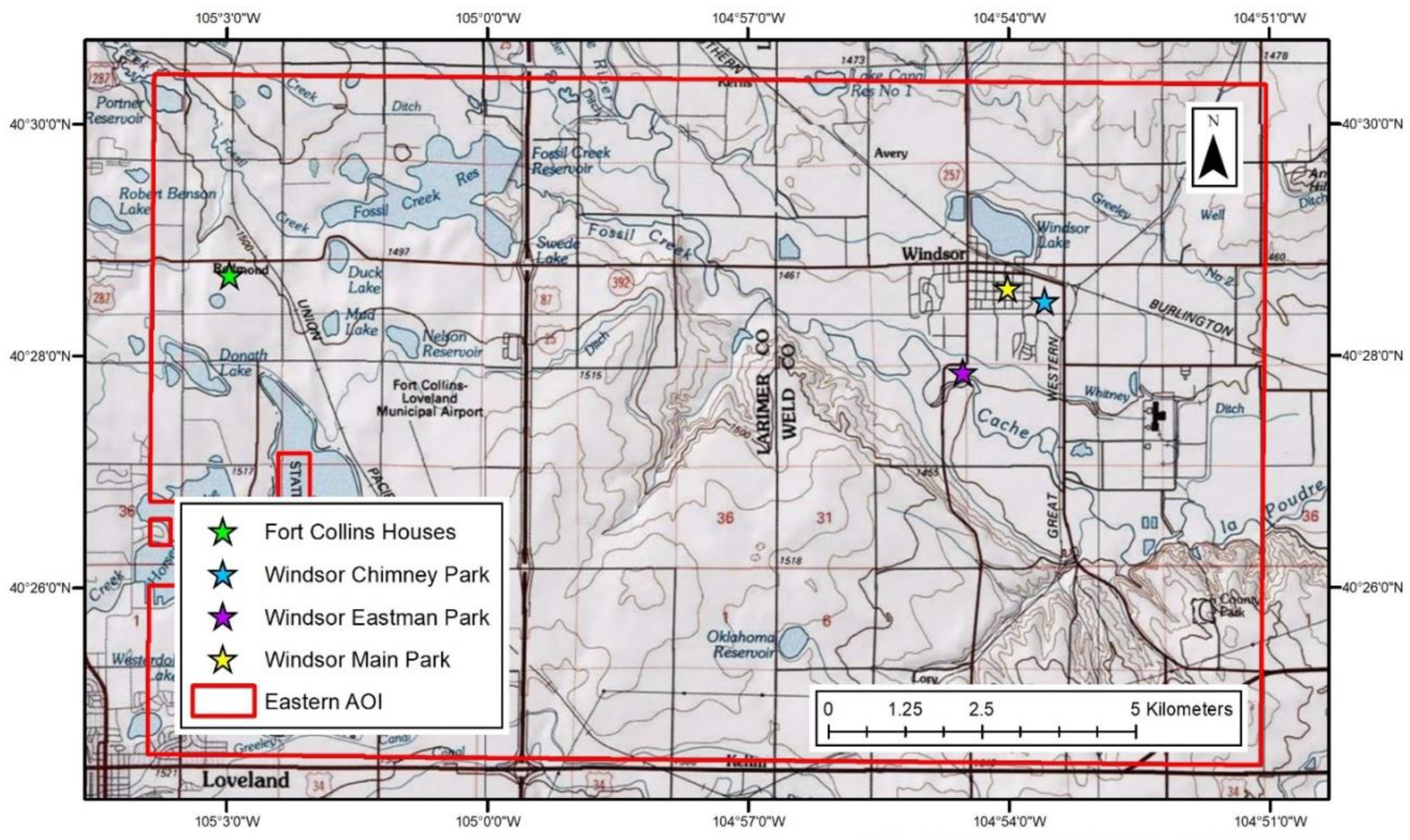
The eastern AOI (Figure 2) included four field sites. The first field site consisted of two houses in the southeastern portion of Fort Collins, Colorado. The remaining field sites were Chimney Park, Windsor Main Park, and Eastman Park, all located within Windsor, Colorado.
The western AOI and eastern AOI have very different landscapes. The western AOI is an area characterized by rugged terrain and high relief, with sage brush and coniferous ecosystems. The eastern AOI is relatively flat and composed of urban areas interspersed with agricultural land. Measurements in the western AOI focused on collecting ground elevation points in the shrubland areas (all BLM plots and WGWVA), using a real-time kinematic (RTK) GNSS, collecting ground elevation points under the tree canopy (BLM plot 5 and the USFS plot) with a total station, measuring tree heights with a total station (BLM plot 5 and the USFS plot), scanning trees with TLS (BLM plot 5 and the USFS plot), scanning structures and hard surfaces with TLS (WGWVA), and collecting UAS imagery (BLM plot 5).
Measurements in the eastern AOI focused on collecting ground elevation points on hard surfaces and grass-covered areas with GNSS, collecting roof points on structures with a total station, and scanning structures with TLS. One parking lot was also scanned with TLS at Eastman Park.

2.1.1. Conventional Surveying Methodology

The GNSS data collection employed a Trimble R8 Model 2 base station with a TDL-450H external radio in combination with a Trimble R8 Model 2 rover and a Trimble R8 Model 3 rover. The Trimble GNSS equipment has a horizontal accuracy of ± 1 cm plus 1 part per million (ppm) root mean square (RMS) 2 cm and a vertical accuracy of ± 2 cm plus 1 ppm RMS 3 cm [19]. All coordinate data were collected in Universal Transverse Mercator Zone 13 North, North American Datum 1983 (2011), North American Vertical Datum 1988 Geoid 12B coordinates. The base station was set to record positional data at 1 s intervals. All base station occupations were at least 2 h in duration. The base station data were downloaded from the base station at the end of occupation. These data were converted to the receiver independent exchange format and post-processed with the National Oceanic and Atmospheric Administration National Geodetic Survey Online Positioning User Service (OPUS) using the static survey protocol after precise satellite orbits were published. The final base station coordinates delivered by the OPUS were used to update all other GNSS points using Trimble Business Center version 3.40 software. GNSS was also used to set control points for a Trimble S6 robotic total station. The Trimble S6 total station has an angular measurement accuracy of 3” and a distance measurement accuracy of ± 3 mm + 2 ppm [20]. The coordinates of these control points were also updated following base station post-processing, which in turn updated all of the points collected with the total station to final coordinates [21].
Throughout the ground truth survey, the position dilution of precision (PDOP) value was very low (mean value of 1.5 and maximum value of 2.7), which indicates excellent satellite condition, as a PDOP of less than 4 is considered as good satellite condition. The GNSS positional accuracy of the ground survey is shown in Table 1. Mean GNSS positional uncertainties evaluated at 95% confidence level were 1.6 cm horizontal and 2.0 cm vertical.

2.1.2. Terrestrial Laser Scanner Methodology

An Optech ILRIS 3D laser scanner equipped with a pan/tilt base was used to conduct the TLS scans. The Optech ILRIS 3D has a raw range accuracy of 7 mm at 100 m and a raw positional accuracy of 8 mm at 100 m. The ILRIS 3D has a 40° × 40° field of view and scans in the near-infrared wavelength of 1535 nm. Using the pan/tilt base allows the scanner to capture up to 10 FOV scan sections, covering 360° horizontally with 2° of horizontal overlap on each end of a scan section [22]. Optech’s Controller PC 5.1.0.1 software, installed on a field laptop computer, was used to operate the scanner and the scan data were stored directly on the laptop. At least four spherical targets were placed in the scanned area to be used for georeferencing. These spherical targets have a 230-mm diameter and were placed on top of leveled range poles. The locations of the spheres’ centers were measured using the total station and a prism [21].
Gexcel JRC 3D Reconstructor 3 ILRIS Scan (64 bit) Version 3.3.1.683 (JRC 3D Reconstructor) software was used to process the scanner data. Raw scan data and images, captured by the scanner, were imported through the JRC 3D Reconstructor software [23]. The JRC 3D Reconstructor software was used to perform an initial “line up” of scan sections. Preprocessing was performed on individual scan sections of a setup. Cloud to cloud registration was performed on individual scan sections of a setup. The registered scan sections were then georeferenced using the spherical targets that were scanned in the field and precisely located with the total station. JRC 3D Reconstructor uses a mean target registration error to display the georeferencing accuracy. The process (“line up,” preprocessing, registration, and georeferencing) was repeated for each scanner setup at a field site. All scan sections for all setups were finely registered through a bundle adjustment or cloud to cloud registration after the final scan setup for an area was georeferenced. A final georeferencing was performed after all scan sections were finely registered together. Minimal manual noise point removal was performed. Finally, all scan sections were then merged into a single point cloud and exported as a LASer (LAS) file [21].

2.2. Three-Plane Intersection and 3D Accuracy Assessment

A three-plane geometrical feature creates a unique intersection point. An intersection point determined from a high accuracy reference dataset can be used to evaluate the accuracy of a lidar point cloud. Since a three-plane object will be used to evaluate the error between two point clouds, we describe the computation method. Each planar point cloud can be considered as a mathematical regression plane defined by a normal vector and a point on the plane. For three planes, the normal vectors are n 1 ,   n 2 ,   n 3 and the points on each plane are x 1 ,   x 2 ,   x 3 . Then the intersection point x 0 is computed by
x 0 = [ ( x 1 · n 1 ) ( n 2 × n 3 ) + ( x 2 · n 2 ) ( n 3 × n 1 ) + ( x 3 · n 3 ) ( n 1 × n 2 ) ] / D
where D is the determinant of the matrix formed by the three direction vectors [24]. This intersection point solution from Equation (1) is completely general if the three planes are mathematically defined. The challenge is to determine the conditions under which a plane can be valid for a sample point cloud and can be used for a lidar accuracy assessment. Kim et al. [18] analyzed this issue extensively in the external uncertainty model approach. In this study, we assume any sampled plane point cloud satisfies the conditions addressed in the external uncertainty model. Consider N-point lidar data X and its covariance matrix Σ ,
X = [ x 1 y 1 z 1 x N y N z N ]   ,   Σ = X t X
The points X are sampled to create a plane. Using the sampled points, a covariance matrix in Equation (2) is computed, followed by an eigen analysis. The third eigenvector of the covariance matrix with smallest eigenvalue is the normal vector to the plane. A point on the plane is computed as a mean point of a point cloud data matrix X . In this manner, we can model three planes from an object out of a reference lidar dataset and the intersection point of the reference data is computed using Equation (1). We consider TLS data to be of sufficiently high accuracy that they can be used as reference data. We can also model another three planes from a comparison lidar dataset whose accuracy is to be evaluated (e.g., airborne lidar data). A new intersection point is computed. The difference between two intersection points represents the error between the two lidar point clouds. In this straightforward method, a regression plane will be completely dependent on how the points are sampled. That means the normal vectors and the point on the plane will be determined solely by the selected points with no other conditions. We call this the “generic three-plane” method.
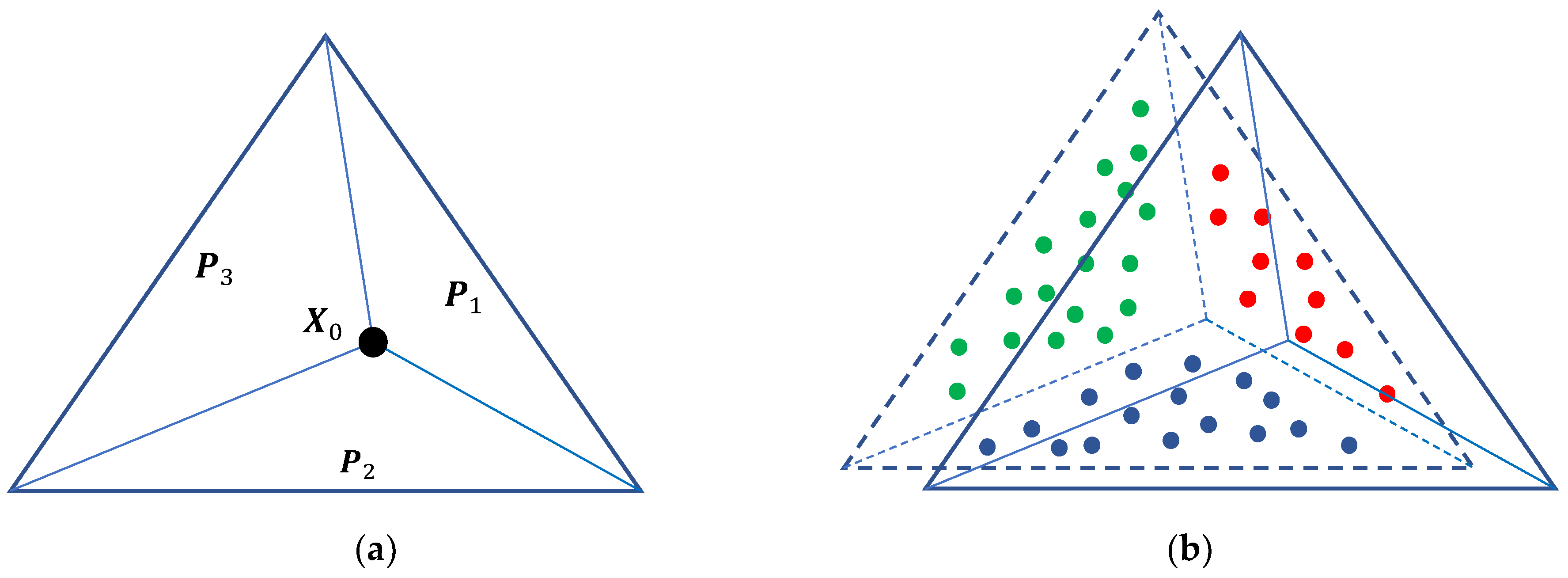
On the other hand, it is reasonable to assume that a reference point cloud and an airborne point cloud have translational error only and no relative rotational error [25]. We call this the “translation only” method as opposed to the “generic three-plane” method. Consider a tetrahedron with three side planes P 1 ,   P 2 ,   P 3 and its intersection point X 0 = [ x 0 , y 0 , z 0 ] illustrated from a downward-looking top view (Figure 3a), where the intersection point X 0 is the highest point. Using the reference dataset, the direction vectors n 1 ,   n 2 ,   n 3 can be accurately determined because we assume the points from the reference data have high precision and high density. Because of the high density, large numbers of individual points in Figure 3a are not shown. If the airborne point cloud has only translational displacement (Figure 3b), we can estimate the displacement ( Δ x , Δ y , Δ z ) using multi-plane least square regression.
There are N 1 , N 2 , and N 3 points sampled to create planes P 1 ,   P 2 ,   P 3 and all the 3D point position vectors in each plane are collected into a position matrix, as follows:
X 1 = [ x 1 y 1 z 1 x N 1 y N 1 z N 1 ] ,   X 2 = [ x 1 y 1 z 1 x N 2 y N 2 z N 2 ] ,   X 3 = [ x 1 y 1 z 1 x N 3 y N 3 z N 3 ]
Using the normal vectors n 1 ,   n 2 ,   n 3 computed from reference data (Figure 3a)
n 1 = [ n 1 x n 1 y n 1 z ] ,   n 2 = [ n 2 x n 2 y n 2 z ] ,   n 3 = [ n 3 x n 3 y n 3 z ] ,
The least square plane regression model is
n i · ( X i X Δ ) = 0 ,    X Δ = X 0 + [ Δ x Δ y Δ z ]
Combining the three planes described in Equation (5) yields a regression model to solve for a linear parameter of the intersection point
M = N · X Δ
where M is an ( N 1 + N 2 + N 3 )-element column vector which combines the three inner products of a direction vector and a point position vector. The M 1 vector is shown below and M 2 , M 3 are defined similarly. N is an ( N 1 + N 2 + N 3 )-row and three-column matrix that comprises plane normal vectors in a way that the first N 1 rows are a repetition of first normal vector, and the second and third normal vectors are filled in similar manner
M 1 = [ n 1 x · x 1 + n 1 y · y 1 + n 1 z · z 1 n 1 x · x N 1 + n 1 y · y N 1 + n 1 z · z N 1 ] ,   M = [ M 1 M 2 M 3 ] , N = [ n 1 x n 1 y n 1 z n 2 x n 2 y n 2 z n 3 x n 3 y n 3 z ]
The solution to Equation (6) is given by
X Δ = ( N t N ) 1 N t M
The 3D error between the comparison lidar point cloud and the reference point cloud is obtained by X Δ X 0 . The difference between two intersection point computations is that the second approach (Equation (5)) uses the normal vectors of the reference planes as a constraint, while its own new normal vectors for the comparison data are computed in the generic three-plane approach (Equation (1)).

2.3. Intraswath and Interswath Analysis

Intraswath analysis applies to the lidar point cloud from single swath data. The following intraswath accuracy measures represent the lidar point cloud quality.

2.3.1. Intraswath Smooth Surface Precision

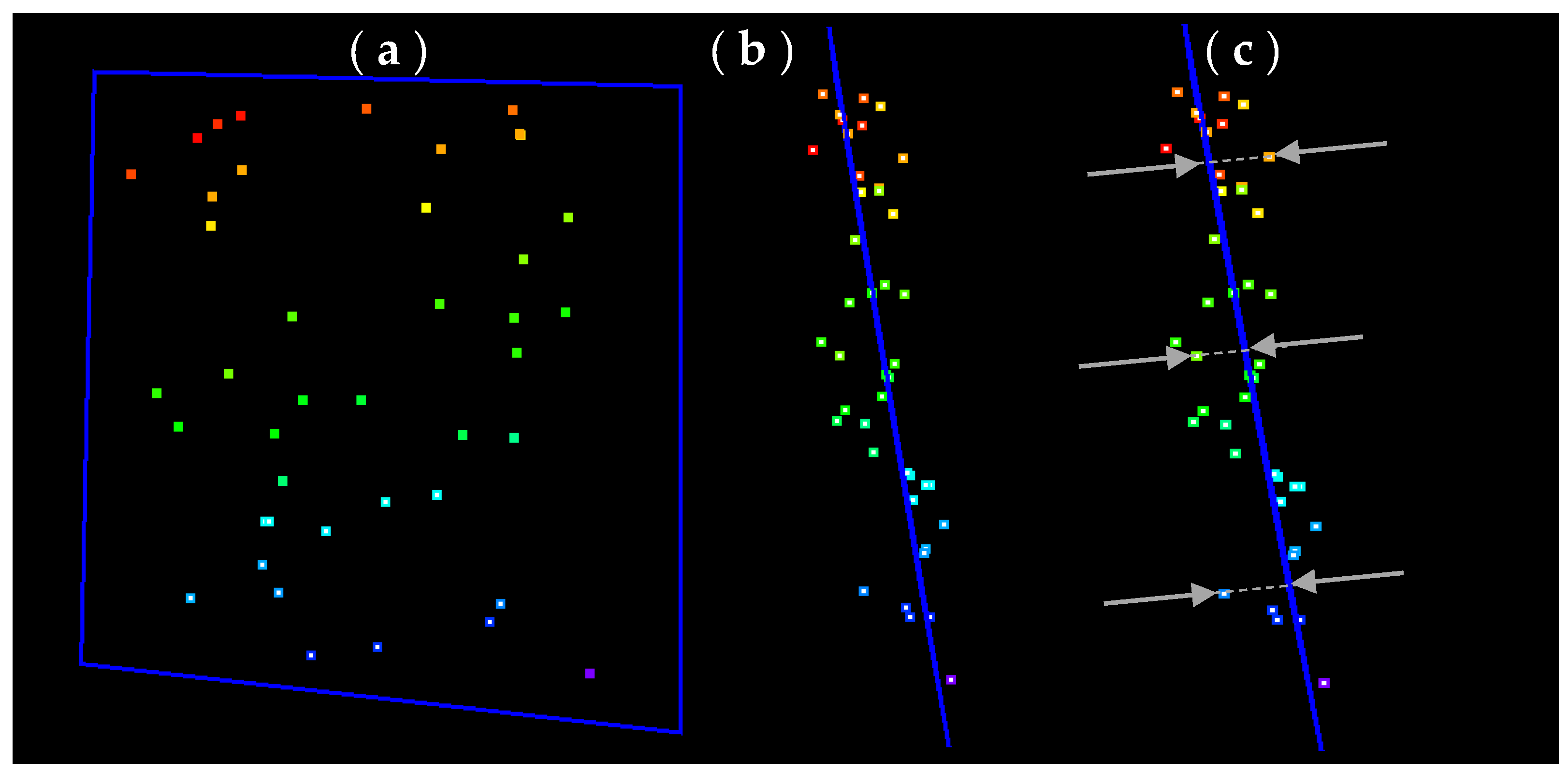
One specific form of smooth surface precision on the raster digital elevation model (DEM) is defined in the LBS [2]. The raster-based DEM, where the lidar point cloud is usually resampled into a 1 m raster based upon points that are classified as ground, is not a raw data format that reveals its fundamental precision. Thus, we suggest using a precision measure based on the point cloud. Assume we sampled N-point lidar data X (Figure 4a). Using a mean point X 0 , re-center the data ( X X 0 ), and compute the covariance matrix Σ = ( X X 0 ) t ( X X 0 ) , then the third eigenvector n 3 from the covariance matrix is the normal vector to the plane (Figure 4b). The next step is to project all the points to the mean plane to compute the point to plane normal distances D (Figure 4c) and the smooth surface precision σ s
D = ( X X 0 ) n 3 ,   σ s = R M S E ( D )
Based on the empirical observations from numerous typical airborne lidar point cloud returns from flat surfaces (e.g., concrete slabs, asphalt shingle roofs) the smooth surface precision σ s is as small as 1 cm for high precision airborne lidar systems, and the value increases for lower end systems. The normal distances for the points in Figure 4 were exaggerated for visualization purposes.

2.3.2. Intraswath Scan Direction Registration

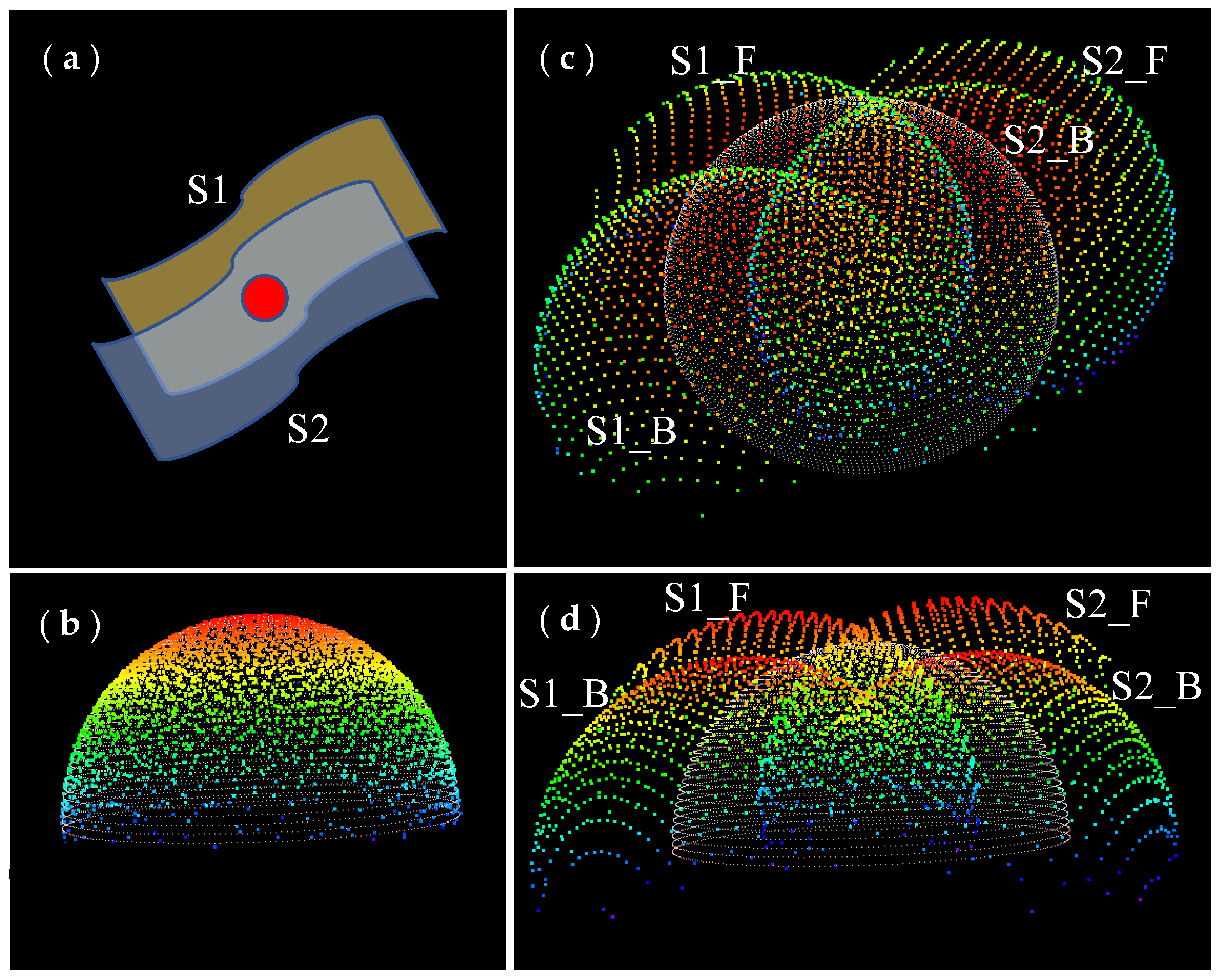
Accurate boresighting is critical for lidar sensors as it is a major source of systematic errors for lidar direct georeferencing. An airborne lidar simulator was used to illustrate the effect of boresighting errors [26]. Two overlapping swaths of lidar point cloud data were created and both swaths contained a hemisphere within the overlapping area (Figure 5a). Several major parameters used to create the hemisphere point clouds in the simulator were: 400 m above ground altitude (AGL) flying height, 100 knots flight speed, a circular scanner with a 40° full field of view (FOV) and a 30 Hz scan frequency, and a 30 KHz laser. These parameters resulted in a 2 PPSM point cloud on the hemisphere, which had a radius of 20 m. Perfect boresighting correction for the hemisphere point cloud is shown in Figure 5b. We applied unrealistically large boresighting errors to demonstrate the resulting amplified georeferencing error. In this case, we applied angular misalignment between sensor frame and inertial measurement unit (IMU) frame by 1° each, and the scan angle offset was also misaligned by 1°. We present the point cloud in nadir view (Figure 5c) and side view (Figure 5d). Not only are the two swaths separated, but so is the lidar point cloud, due to the different scan directions being further separated.
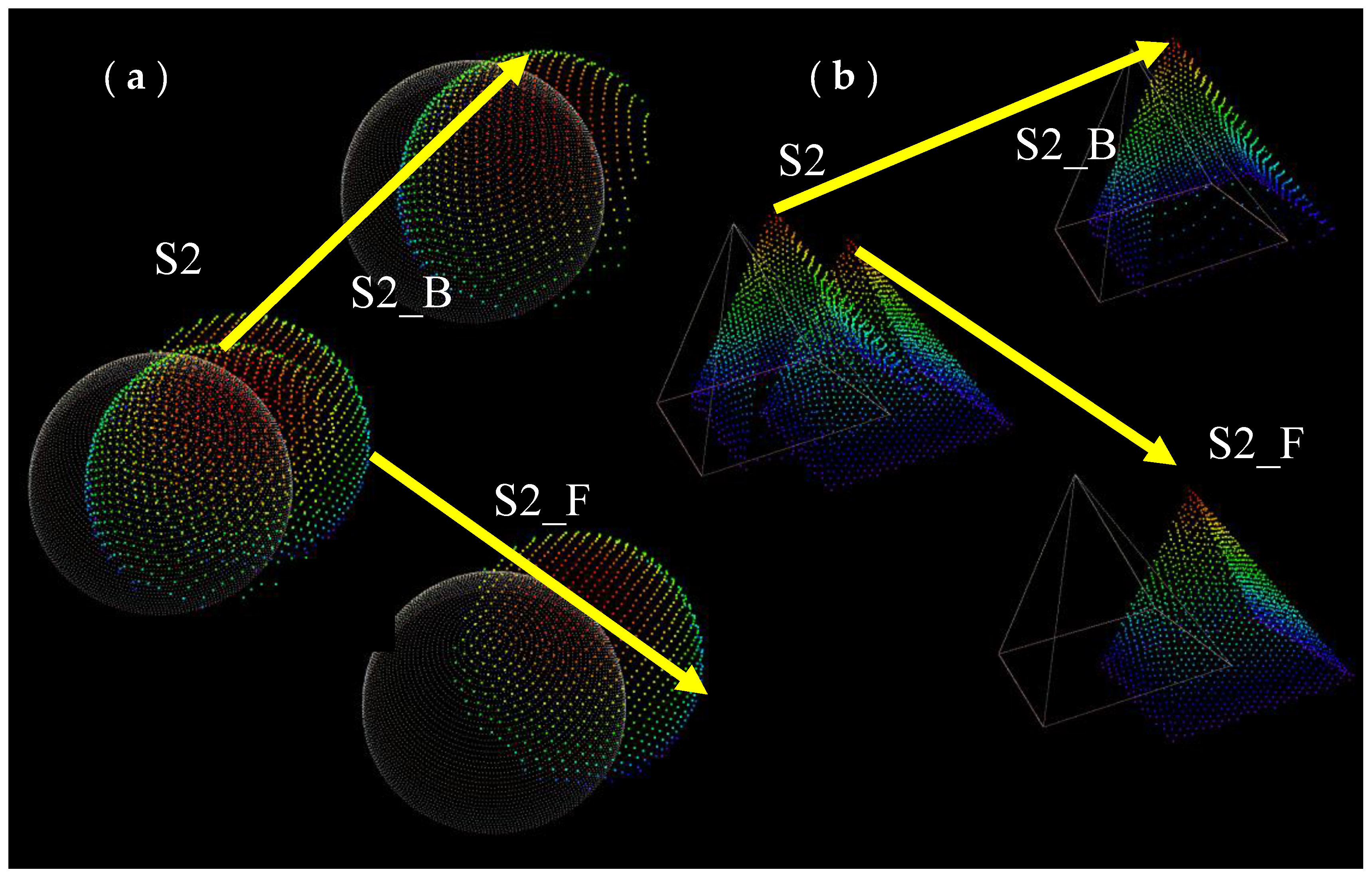
Figure 6a shows only the second swath of the nadir view (Figure 5c). Due to the boresighting errors, the point cloud in the second swath made it appear as if there were two hemispheres. This is because the range returns from the forward scanned laser pulses and backward scanned laser pulses are incorrectly georeferenced due to the boresighting errors. Figure 6b shows a simulated point cloud with a pyramid object instead of a hemisphere. A pyramid allows for a three-plane combination. We can compute an intersection point from three planes using only the forward scanned point cloud and compute a second intersection point from three planes using the backward scanned point cloud. Then, we can compare the two intersection points to evaluate the displacement, which is the intraswath error due to opposite scan directions. We demonstrate this method using a building point cloud from the CountryMapper airborne lidar sensor.

2.3.3. Interswath Consistency

Interswath overlap consistency reveals the fundamental quality of the lidar point cloud because it establishes the quality and accuracy limits of all downstream data and products. Boresighting or other calibration errors result in substantial interswath differences. A raster-based interswath method and requirement is suggested by the USGS [2]. It guides the creation of difference rasters and the calculation of RMSD in the vertical direction (RMSDz). We used a point cloud-based interswath difference method using geometric features (e.g., three-plane objects shown in Section 2.2) in the overlapping area from two swaths. The method is identical to the intraswath error assessment using two opposite scan directions, except interswath consistency uses two overlapping swaths. This method is demonstrated in Section 3.2.

2.4. Absolute Vertical Accuracy

Determining absolute vertical accuracy is a practical choice because assessing horizontal accuracy is a difficult task with point cloud data. Thus, it is important to make sure that checkpoints satisfy recommended conditions to limit substantial additional errors caused by horizontal uncertainty. There are several recommended conditions [2]. Checkpoints shall be surveyed in clear, open areas (which typically produce only single lidar returns) for non-vegetated vertical accuracy (NVA) assessment. Checkpoints for vegetated vertical accuracy (VVA) assessment shall be surveyed in vegetated areas, which typically produce multiple returns. Suitable checkpoint survey areas should be a homogeneous area with a minimum size of ( A N P S 5 ) 2 , with less than one-third of the required RMSEz deviation from a low-slope (<10 degrees) plane, where ANPS is the aggregate nominal point spacing [2]. The ANPS value for the CountryMapper airborne lidar in this project was about 70 cm, which resulted from a 2 PPSM point density. Thus, the NVA checkpoints were surveyed on flat areas larger than 3.5 m × 3.5 m.
The NVA at the 95% confidence level in non-vegetated terrain is approximated by multiplying the accuracy value of the vertical accuracy class, or RMSEz, by 1.9600. The NVA, based on the RMSEz multiplier, should be used only in non-vegetated terrain where elevation errors typically follow a normal error distribution. RMSEz-based statistics should not be used to estimate vertical accuracy in vegetated terrain or where elevation errors often do not follow a normal distribution [1].
The VVA at the 95% confidence level in vegetated terrain is computed as the 95th percentile of the absolute value of vertical errors in all vegetated land cover categories combined, including tall weeds and crops, brush lands, and fully forested areas. Both the RMSEz and 95th percentile methodologies specified above are currently widely accepted in standard practice and have been proven to work well for typical elevation datasets derived from current technologies [1].

3. Results

3.1. Intraswath Smooth Surface Precision

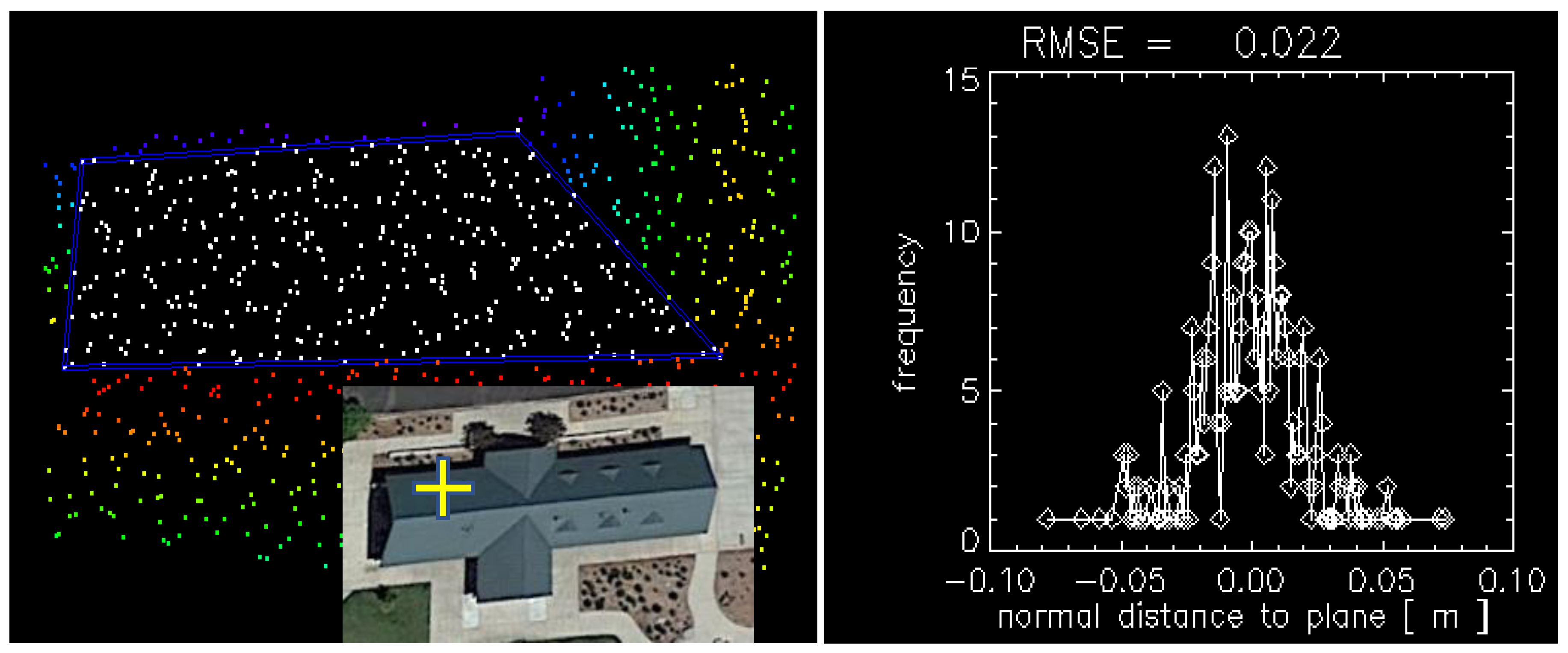
To evaluate intraswath smooth surface precision, we used a park office building in Eastman Park in Windsor, Colorado, as shown in Figure 7. The point cloud from the roof plane marked by the yellow cross was sampled. The histogram of the normal distance to the plane is shown. The RMSE 2.2 cm was calculated using Equation (9). There were 60 plane features extracted in the 3D absolute accuracy study. Each plane yielded smooth surface precision and the average of the 60 planes was 2.5 cm.

3.2. Intraswath Difference between Opposite Scan Direction

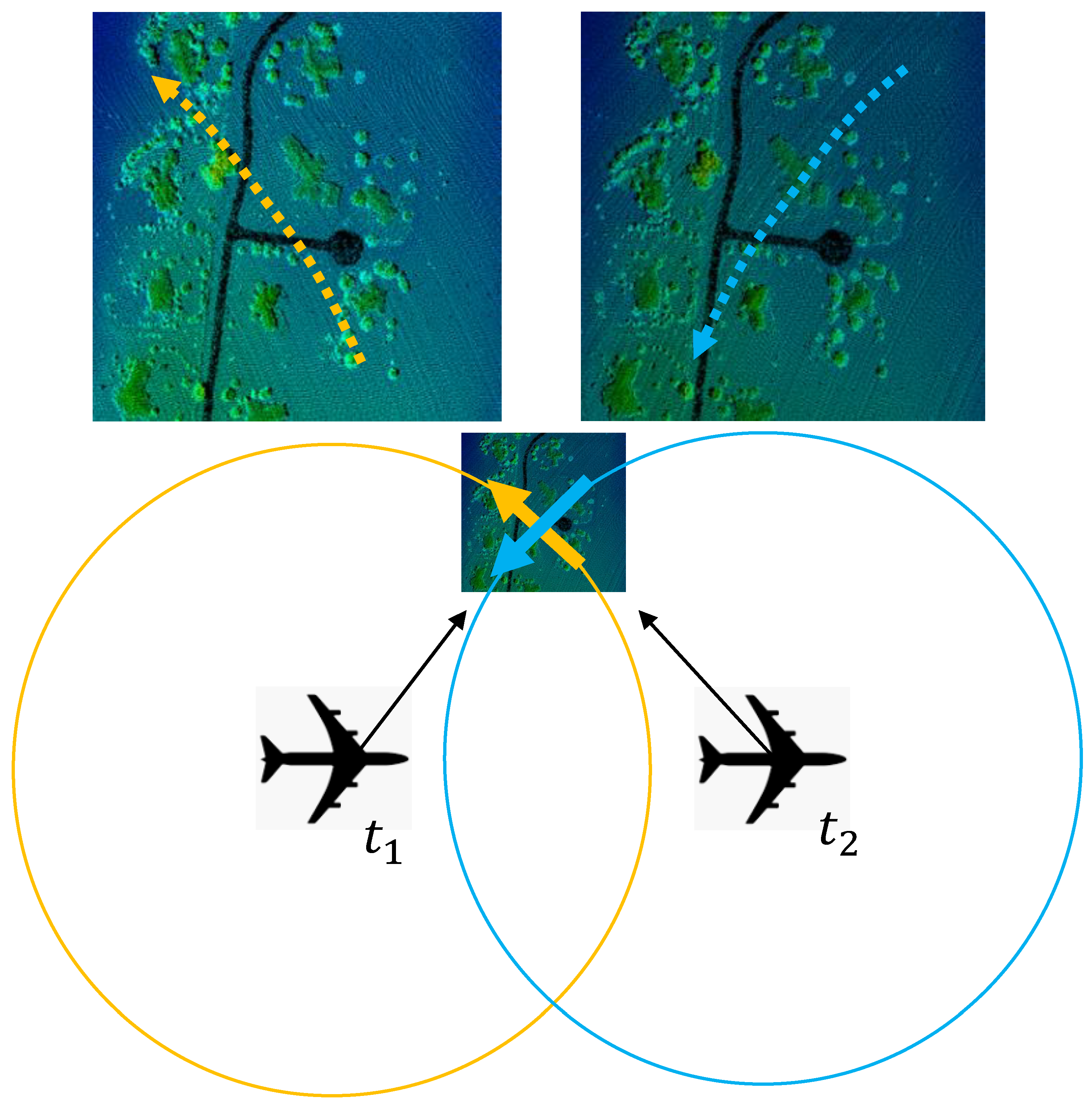
The CountryMapper lidar uses a Palmer scanner that creates a generally elliptical scan pattern. Any surface spot is scanned twice; once at time t 1 in a forward scan segment, and once at time t 2 in a backward scan segment (Figure 8). Thus, the local area point cloud can be separated into forward and backward scan groups. The partial scan pattern is clearly visible as an arc in a different direction, as is illustrated by the yellow and cyan arrows in Figure 8. The combination of both makes a single swath.
As demonstrated in Figure 6, if there is a substantial boresighting error, point clouds from opposite scan directions can have displacement. Groups of point cloud data were sampled to form three-plane combinations for backward and forward scans separately (Figure 9). Two intersection points are computed and compared to get the intraswath difference Δ x = 0.2   cm ,   Δ y = 3   cm ,   Δ z = 1.6   cm .

3.3. Interswath Consistency

Since interswath consistency is the relative difference between two swaths, and each swath consists of both scan directions (Figure 10), the point density is twice as high when compared to the separated scan directions in Figure 9. Two intersection points are computed and compared to get the interswath difference Δ x = 1.4   cm ,   Δ y = 2   cm ,   Δ z = 2   cm .

3.4. Absolute Vertical Accuracy

3.4.1. Nonvegetated Vertical Accuracy

The NVA analysis was performed against survey grade GNSS ground points from the urban locations in the eastern AOI because the conditions for the NVA checkpoints are mostly satisfied on the man-made surfaces in the urban areas (Figure 11).
We performed NVA analysis of CountryMapper lidar point clouds on three sites, the results of which are summarized in Table 2.

3.4.2. Vegetated Vertical Accuracy

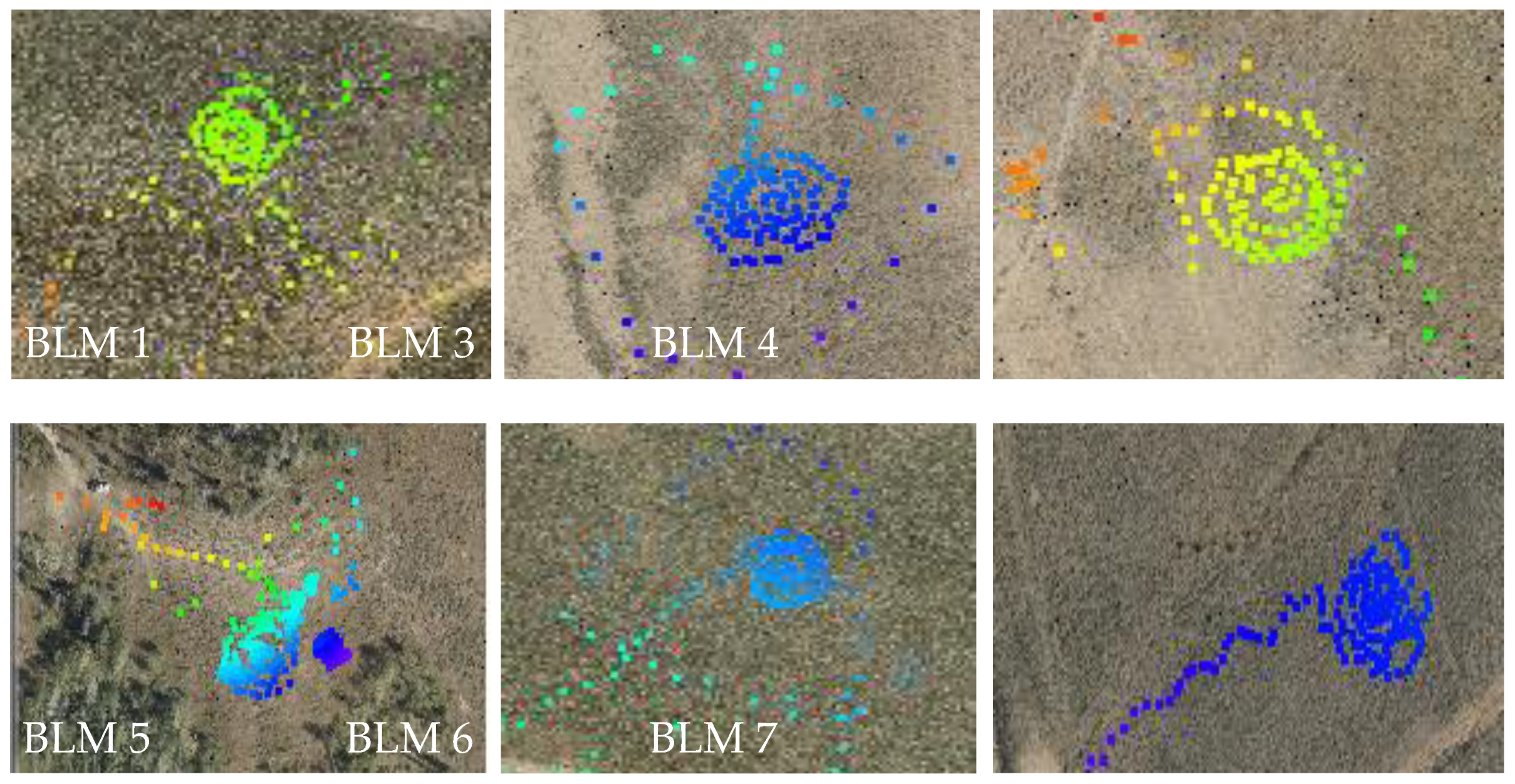
The VVA analysis was performed against survey grade GNSS ground points from the BLM-managed land in the western AOI. The rover points are shown with their roughly concentric distribution centered around BLM plot coordinates in Figure 12.
We performed the VVA analysis of CountryMapper lidar point clouds. Additionally, VVA analyses were conducted on UAS lidar point clouds and structure from motion (SfM) point clouds collected by the USGS National UAS Project Office (NUPO), at the request of the BLM, over the same plots [21]. The results for all six VVA analyses are shown in Table 3. The UAS lidar data were not produced for the BLM2 site, thus they are not shown in Table 3.

3.5. D Absolute Accuracy Analysis

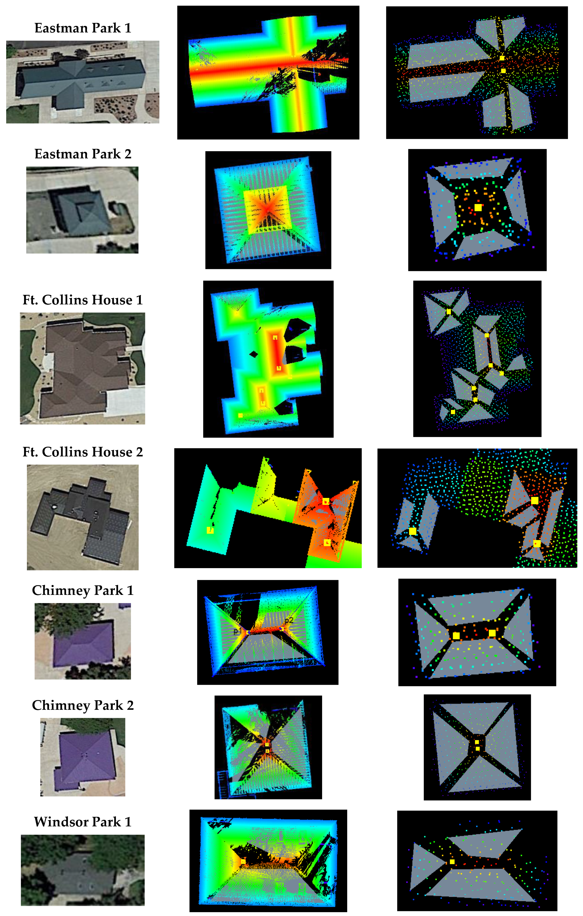
A three-plane intersection point is a well-defined geometric feature. One set of three-plane features was defined in TLS point clouds and the other set was defined in the airborne lidar point cloud. In the case of the dataset “Eastman Park 1”, two three-plane sets were defined, and thus two intersection points were computed from both the TLS and airborne data (Figure 13). By comparing the corresponding intersection points, we get an error ( Δ x , Δ y , Δ z ) vector for each intersection point, which is shown in Table 4. “Ft. Collins House 1” had a complex, multi-faceted roof structure, thus it was possible to extract as many as eight intersection points. In this manner, a total of 20 corresponding intersection points were collected in the field data and the error statistics for the comparison to the airborne data are shown in Table 5.

4. Discussion

The 2.2 cm RMSE intraswath smooth surface precision value (Figure 7) is excellent based on the USGS quality level (QL) 2 requirement (<6 cm) in the LBS. Very small intraswath differences between opposite scan directions (Figure 9) were observed. Again, compared to USGS QL 2 requirements (<6 cm,) these results indicate there was minimal systematic error and the CountryMapper boresighting quality was good. The differences between two intersection points in the interswath analysis shown in Figure 10 (all 2 cm or less) were also very small, considering the USGS QL 2 requirement (<8 cm).
The NVA mean is approximately 2 cm and the RMSE is less than 3 cm, which is also very low (Table 2) compared to the USGS LBS requirement (<10 cm). Since the mean value (~2 cm) is computed by subtracting the lidar point elevations from the ground truth point elevations, it means that the airborne lidar data are approximately 2 cm lower than the GNSS-measured “true” elevation. Having this in mind, the negative VVA mean values make physical sense (Table 3) because the lidar return from the vegetation is a little bit earlier (higher elevation) than ground surface (lower elevation). The VVA mean values from airborne lidar range from −3 cm to −8 cm, depending on the BLM sites. The RMSEz values are 3–5 cm, which is well within the USGS LBS QL 2 requirement (<10 cm).
The VVA analysis of the UAS lidar data showed a reasonable mean shift and RMSEz (Table 3). Although we included a VVA analysis using the SfM point clouds, the mean shift and RMSEz were substantially larger than for the CountryMapper and UAS lidar data, which implies that the SfM data were not well calibrated. The SfM data in this field campaign were collected mainly to add RGB color information to the point cloud rather than to produce a reference dataset. While the quality of the UAS lidar data could be considered good enough to be used as reference ground truth datasets that have the potential to replace time-consuming GNSS point measurements, the SfM data produced in this field campaign lack accuracy. However, SfM data from well-calibrated mapping grade cameras should be able to create point clouds accurate enough to be used as reference datasets. We can take advantage of many available man-made geometric features, if available. In mostly natural areas, ground control targets need to be placed before SfM for the geo-calibration.
The coincident evaluation of the horizontal absolute accuracy and the vertical absolute accuracy is made possible by extracting unique comparison points from geometric features, e.g., the intersection point from a three-plane object. We found multi-faceted roof objects and calculated conjugate intersection points from the reference TLS data and from the airborne data. The differences give error ( Δ x , Δ y , Δ z ) vectors that were compiled into Table 4 and Table 5 gives the mean shift and RMSE for each axis. The mean shift along the x-axis is substantially large (~20 cm) when compared to the y-axis (7–8 cm) and z-axis (3–6 cm) shifts. Based upon the general rule described in the ASPRS positional accuracy standard [1], the mean error should be less than 25% of the specified RMSE value. The suggested mean error becomes 2.5 cm, based on the 10-cm RMSE specification. The mean errors of the airborne lidar data were quite large, which had to be addressed during the raw data correction using ground control points by the data provider. Nevertheless, ASPRS specifies that the correction of significant systematic errors (or biases) is the responsibility of the data provider [1].
The intersection point from the three-plane object is affected by the point cloud sampling for each individual plane. The potential variability caused by the arbitrary planar point cloud sampling needs to be addressed to avoid excessive additional error caused by improper sampling. For instance, too few points may cause a larger deviation of the modeled plane from the true plane. The number of points is determined by point density and the dimension of the planar feature. Even if the same number of points was used, if the smooth surface precision is low, the error will be larger. These factors are incorporated into a general external uncertainty model [18] and the model was applied to all planar features in the current analysis to make sure the modeled planes introduced an external error smaller than the preset threshold (2 cm positional uncertainty at one standard deviation).
Along with the validity conditions of the plane, the availability of three-plane man-made features is a practical concern, especially in a region where these objects are sparse or non-existent. In that case, a tetrahedron target whose dimension is determined based on an external uncertainty model can be placed prior to the airborne lidar campaign.
The 3D accuracy results were calculated using generic three-plane and translation only methods, which were described in the methods Section 2.2. The standard deviation of the horizontal error is not negligibly small, evidenced from relatively large RMSE values. However, the RMSE values reflecting the variation are still within the USGS LBS QL 2 requirement. Regarding the methods, we simply assumed the translation only situation (no rotational error) was the case between the TLS data and airborne point cloud. This assumption was supported by the fact that the intraswath and interswath errors were almost negligible, especially when compared to the error requirement specifications. Thus, method two (translation error only) was conceptually preferable, because the direction vector from the reference data was used as a constraint for comparison to the airborne data. The results between the two methods were less than 1 cm horizontal and less than 3 cm vertical.

5. Conclusions

This paper reports on several different methods used to measure the accuracy of the lidar point cloud data collected for the NAIP/3DEP pilot project. All the results appeared to satisfy the USGS LBS QL 2 requirements, although some of the point cloud vector-based methods presented in this paper are different from the raster-based methods suggested in LBS. The 2 PPSM point cloud data appeared to be minimally noisier ( σ s = 2.2   cm ) than the latest low altitude lidar point cloud (e.g., σ s = 1   cm USGS Inland Bathy Lidar from Kootenai River [27] with 400 m flying height), even though the flight altitude was relatively high at 3.6 km AGL. The flying altitude was designed as an optimal solution to meet the requirements for both NAIP areal coverage and 3DEP QL 2 lidar point density. The accuracy of the airborne point cloud is good enough to create a standard 1 m digital elevation model (DEM), however, it lacks the quality and precision desired for 3D object modeling, which requires at least QL 1 (>8 PPSM) data. Thus, the airborne lidar point cloud appears to have met the lidar requirements for the NAIP and 3DEP project, based on the QL 2 category.
We used the 3D absolute accuracy assessment, based on geometric features, as a standard accuracy assessment practice. This study is another experimental example, such as we reported previously [18], where we focused more on the valid conditions for using planar features in terms of their total propagated uncertainty (TPU), size, and the density of points on the plane.
A limitation of this 3D accuracy study was that the number of checkpoints was not large enough. TLS ground truth data collection at many different sites, with reasonably good spatial distribution, is more difficult than measuring conventional checkpoints. UAS lidar data could potentially expedite ground truth surveys in the future, both in terms of the quantity of checkpoints collected and the speed of the data collection. This will be a topic for our next study. Despite the limitations, we demonstrated that the practice of assessing the 3D absolute accuracy of lidar point clouds is a viable option during the NAIP/3DEP campaign and we will continue to work on improving ground survey protocols.

Author Contributions

Conceptualization, M.K.; methodology, M.K.; software, S.P. and M.K.; validation, S.P.; formal analysis, M.K., S.P.; investigation, J.I.; resources, J.D.; data curation, J.D., J.I., M.K., M.B. (Mark Bauer), M.B. (Matthew Burgess), and A.S.; writing—original draft preparation, M.K., C.M., J.I; writing—review and editing, J.D. and G.S.; visualization, S.P.; supervision, G.S.; project administration, G.S.; funding acquisition, G.S. All authors have read and agreed to the published version of the manuscript.

Funding

This research was funded by the USGS National Geospatial Program (NGP) 3DEP and USDA NRCS NGCE.

Conflicts of Interest

The authors declare no conflict of interest.

References

  1. ASPRS. ASPRS Positional Accuracy Standards for Digital Geospatial Data. Photogramm. Eng. Remote Sens. 2015, 81, A1–A26. [Google Scholar] [CrossRef]
  2. Heidemann, H.K. Lidar Base Specification; (Version 1.3, February 2018); Book 11; Chapter B4; U.S. Geological Survey Standards: Reston, VA, USA, 2018; p. 101. [Google Scholar] [CrossRef] [Green Version]
  3. NDEP (National Digital Elevation Program). National Digital Elevation Program, Guidelines for Digital Elevation Data; Version 1.0.; ASPRS: Bethesda, MD, USA, 2004. [Google Scholar]
  4. FGDC (Federal Geographic Data Committee). Geospatial Positioning Accuracy Standards. Part 3: National Standard for Spatial Data Accuracy; FGDC-STD-007.3-1998; USGS: Reston, VA, USA, 1998. [Google Scholar]
  5. FEMA. Guidelines and Standards for Flood Hazard Mapping Partners; FEMA: Washington, DC, USA, 2003.
  6. Habib, A.; Bang, K.I.; Kersting, A.P.; Lee, D.C. Error budget of LiDAR systems and quality control of the derived data. Photogramm. Eng. Remote Sens. 2009, 75, 1093–1108. [Google Scholar] [CrossRef]
  7. Tulldahl, M.; Bissmarck, F.; Larsson, H.; Grönwall, C.; Tolt, G. Accuracy evaluation of 3D lidar data from small UAV. In Proceedings of the SPIE 9649, Electro-Optical Remote Sensing, Photonic Technologies, and Applications IX, Auditorium Antoine de Saint-Exupery, Toulouse, France, 21–22 September 2015; p. 964903. [Google Scholar]
  8. Borrmann, D.; Elseberg, J.; Kai, L.; Nüchter, A. The 3D Hough Transform for plane detection in point clouds: A review and a new accumulator design. 3D Res. 2011, 2, 1–13. [Google Scholar] [CrossRef]
  9. Georgiev, K.; Creed, R.T.; Lakaemper, R. Fast plane extraction in 3d range data based on line segments. In Proceedings of the Intelligent Robots and Systems (IROS), IEEE/RSJ International Conference, San Francisco, CA, USA, 25–30 September 2011; pp. 3808–3815. [Google Scholar]
  10. Vosselman, G.; Gorte, B.G.; Sithole, G.; Rabbani, T. Recognising structure in laser scanner point clouds. Int. Arch. Photogramm. Remote Sens. Spat. Inf. Sci. 2004, 46, 339–344. [Google Scholar]
  11. Rabbani, T.; van den Heuvel, F.A.; Vosselman, G. Segmentation of point clouds using smoothness constraint. In Proceedings of the International Archives of Photogrammetry, Remote Sensing & Spatial Information Sciences, Goa, India, 25–30 September 2006. [Google Scholar]
  12. Tarsha-Kurdi, F.; Landes, T.; Grussenmeyer, P.; Koehl, M. Model-driven and data-driven approaches using LIDAR data: Analysis and comparison. In Proceedings of the Photogrammetric Image Analysis, Munich, Germany, 19–21 September 2007; pp. 87–92. [Google Scholar]
  13. Chen, L.; Zhao, S. Building detection in an urban area using LiDAR data and quickbird imagery. Int. J. Remote Sens. 2012, 33, 5135–5148. [Google Scholar] [CrossRef]
  14. Li, Y.; Wu, H.; An, R.; Xu, H.; He, Q.; Xu, J. An improved building boundary extraction algorithm based on fusion of optical imagery and LIDAR data. Optik 2013, 124, 5357–5362. [Google Scholar] [CrossRef]
  15. Zhou, G.; Zhou, X. Seamless Fusion of LiDAR and Aerial Imagery for Building Extraction. IEEE Trans. Geosci. Remote Sens. 2014, 52, 7393–7407. [Google Scholar] [CrossRef]
  16. Zarea, A.; Mohammadzadeh, A. A Novel Building and Tree Detection Method from LiDAR Data and Aerial Images. IEEE J. Sel. Top. Appl. Earth Obs. Remote Sens. 2016, 9, 1864–1875. [Google Scholar] [CrossRef]
  17. Krishnamachari, S.; Chellappa, R. Delineating buildings by grouping lines with MRFs. IEEE Trans. Image Process. 1996, 5, 164–168. [Google Scholar] [CrossRef] [PubMed]
  18. Kim, M.; Park, S.; Danielson, J.; Irwin, J.; Stensaas, G.; Stoker, J.; Nimetz, J. General External Uncertainty Models of Three-Plane Intersection Point for 3D Absolute Accuracy Assessment of Lidar Point Cloud. Remote Sens. 2019, 11, 2737. [Google Scholar] [CrossRef] [Green Version]
  19. Trimble Navigation Limited. Trimble R8 GNSS and R6/5800 GPS Receivers User Guide (Revision A); Trimble Navigation Limited: Dayton, OH, USA, 2008. [Google Scholar]
  20. Trimble Navigation Limited. Trimble S6 Total Station Datasheet; Trimble Navigation Limited: Dayton, OH, USA, 2013. [Google Scholar]
  21. Irwin, J.R.; Sampath, A.; Kim, M.; Bauer, M.A.; Burgess, M.A.; Park, S.; Danielson, J.J. Country Mapper Sensor Validation Survey Data: U.S. Geological Survey Data Release. 2020. Available online: https://usgs.ornl.gov/metadata/catalog/html/Earth_Resources_Observation_and_Science_%28EROS%29_Center/5e5d679ae4b01d50924f2d23.html (accessed on 17 May 2020). [CrossRef]
  22. Optech Incorporated. Optech ILRIS-3D; Optech Inc.: Toronto, ON, Canada, 2006. [Google Scholar]
  23. Gexel. JRC 3D Reconstructor Software Manual; Gexel: Brescia, Italy, 2017. [Google Scholar]
  24. Gellert, W.; Gottwald, S.; Hellwich, M.; Kästner, H.; Künstner, H. VNR Concise Encyclopedia of Mathematics, 2nd ed.; Van Nostrand Reinhold: New York, NY, USA, 1989. [Google Scholar]
  25. Wilkinson, B.; Lassiter, H.A.; Abd-Elrahman, A.; Carthy, R.R.; Ifju, P.; Broadbent, E.; Grimes, N. Geometric Targets for UAS Lidar. Remote Sens. 2019, 11, 3019. [Google Scholar] [CrossRef] [Green Version]
  26. Kim, M. Airborne Waveform Lidar Simulator Using the Radiative Transfer of a Laser Pulse. Appl. Sci. 2019, 9, 2452. [Google Scholar] [CrossRef] [Green Version]
  27. U.S. Geological Survey. USGS Lidar Point Cloud ID KootenaiRiver 2017 KRTH 0031: U.S. Geological Survey; USGS: Reston, VA, USA, 2020.
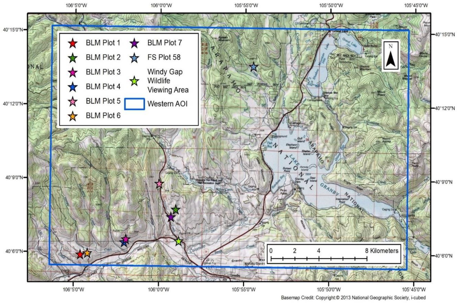
Figure 1. Map of the western AOI field sites.
Remotesensing 12 01974 g001
Figure 2. Map of the eastern AOI field sites.
Remotesensing 12 01974 g002
Figure 3. Lidar 3D absolute error based on three-plane intersection using least square regression. (a) Three-plane object from reference TLS data. (b) Airborne data with translational error only. The red, blue, and green dots are sampled points for planes P 1 ,   P 2 ,   P 3 , respectively.
Remotesensing 12 01974 g003
Figure 4. Smooth surface precision. (a) Selected points for a plane modeling. (b) Side view projected along the regression plane. (c) Normal distances from points to the plane with three example points.
Remotesensing 12 01974 g004
Figure 5. Boresighting simulation. (a) Overlapping two swaths S1 and S2. (b) Point cloud of a hemispherical object in a perfect boresighting correction. (c) Nadir view of the point cloud in a large boresighting misalignment error further separated to forward (F) and backward (B) scanned point cloud. (d) Side view of the point cloud of (c) in 3D perspective. The true target hemisphere is represented using small white dots in panels (c,d).
Remotesensing 12 01974 g005
Figure 6. Intraswath boresighting error shown in opposite scan direction. Swath 2 data shows two apparently misaligned targets due to boresighting error. The arrows indicate the separated forward and backward scanned point cloud. (a) Swath 2 separated into forward and backward scan directions. (b) Same situation as hemisphere, but with a pyramid object.
Remotesensing 12 01974 g006
Figure 7. Illustration of intraswath smooth surface precision.
Remotesensing 12 01974 g007
Figure 8. Point cloud from opposite scan direction.
Remotesensing 12 01974 g008
Figure 9. Three-plane pair sampled from separated point clouds due to opposite scan direction.
Remotesensing 12 01974 g009
Figure 10. Illustration of interswath consistency.
Remotesensing 12 01974 g010
Figure 11. GNSS rover checkpoints for NVA analysis.
Remotesensing 12 01974 g011
Figure 12. GNSS rover checkpoints for VVA analysis.
Remotesensing 12 01974 g012
Figure 13. Three-plane intersection samples, high PPSM TLS data (middle column), low PPSM CountryMapper lidar data (third column). The intersection points are shown as yellow points.
Remotesensing 12 01974 g013
Table 1. GNSS positional accuracy.
Granby AreaFort Collins HousesMain and Chimney ParksEastman ParkAll Areas
Min PDOP1.2141.0281.1531.3491.028
Max PDOP2.7292.2901.8262.0932.729
Mean PDOP1.6531.4681.3611.5561.611
Min Hor. Precision (95%)0.0120.0110.0120.0140.011
Max Hor. Precision (95%)0.0320.0230.0240.0220.032
Mean Hor. Precision (95%)0.0160.0160.0150.0160.016
Min Vert. Precision (95%)0.0150.0140.0140.0170.014
Max Vert. Precision (95%)0.0480.0300.0290.0280.048
Mean Vert. Precision (95%)0.0230.0180.0190.0200.022
Table 2. NVA analysis results in meters.
SitesRover–Lidar
MeanRMSE(z)
Eastman Park0.02090.0245
Ft Collins Houses0.02380.0287
Windsor Park & Chimney Park0.02210.0135
Table 3. VVA analysis results in meters.
SitesRover–LidarRover–UAS LidarRover–SfM
MeanRMSE(z)MeanRMSE(z)MeanRMSE(z)
BLM1−0.03750.0315−0.02640.0222−0.29120.0854
BLM3−0.08500.0434−0.06880.0301−0.14710.0512
BLM4−0.06330.0306−0.08450.0309−0.12900.0562
BLM5−0.04330.0518−0.04530.0269−0.13330.0737
BLM6−0.02980.0284−0.00270.0212−0.16020.0794
BLM7−0.04950.0448−0.01110.0215−0.22260.0693
Table 4. 3D absolute analysis results in meters.
Method 1: Generic Three-PlaneMethod 2: Translation Only
DxDyDzDxDyDz
Eastman Park 1-Point 10.2630.1330.0580.2560.1180.039
Eastman Park 1-Point 20.2270.1580.0290.2460.1540.039
Eastman Park 2-Point 10.2680.0970.0860.2300.1590.013
Eastman Park 2-Point 20.2780.1090.0810.2220.1480.017
Ft Collins House 1-Point 10.2270.2010.0940.2400.1550.022
Ft Collins House 1-Point 20.2450.1040.0980.2380.1710.022
Ft Collins House 1-Point 30.2150.1350.0640.2350.1600.025
Ft Collins House 1-Point 40.2290.0990.0650.2420.1090.025
Ft Collins House 1-Point 50.2360.0800.0280.2310.1180.033
Ft Collins House 1-Point 60.1870.2410.0610.2320.0830.032
Ft Collins House 1-Point 70.2250.0420.0520.2280.1140.032
Ft Collins House 1-Point 80.2460.1560.0760.2190.0940.017
Ft Collins House 2-Point 10.2290.0960.0600.2180.0580.051
Ft Collins House 2-Point 20.1810.0090.0490.2540.1670.067
Ft Collins House 2-Point 30.116−0.0810.0750.237−0.0670.061
Chimney Park 1-Point 10.166−0.0420.0700.159−0.1170.022
Chimney Park 1-Point 20.089−0.0120.0790.134−0.1200.022
Chimney Park 2-Point 10.2570.0920.0610.2030.0000.036
Chimney Park 2-Point 20.2580.0110.0610.2030.0020.036
Windsor Park 1-Point 10.118−0.0340.0630.160−0.0280.060
Table 5. 3D absolute error statistics in meters.
Method 1: Generic Three-PlaneMethod 2: Translation Only
DxDyDzDxDyDz
Mean0.2130.0800.0660.2190.0740.034
RMSE0.0540.0840.0180.0330.0960.016