Abstract
Accurate maps of regional surface water features are integral for advancing ecologic, atmospheric and land development studies. The only comprehensive surface water feature map of Alaska is the National Hydrography Dataset (NHD). NHD features are often digitized representations of historic topographic map blue lines and may be outdated. Here we test deep learning methods to automatically extract surface water features from airborne interferometric synthetic aperture radar (IfSAR) data to update and validate Alaska hydrographic databases. U-net artificial neural networks (ANN) and high-performance computing (HPC) are used for supervised hydrographic feature extraction within a study area comprised of 50 contiguous watersheds in Alaska. Surface water features derived from elevation through automated flow-routing and manual editing are used as training data. Model extensibility is tested with a series of 16 U-net models trained with increasing percentages of the study area, from about 3 to 35 percent. Hydrography is predicted by each of the models for all watersheds not used in training. Input raster layers are derived from digital terrain models, digital surface models, and intensity images from the IfSAR data. Results indicate about 15 percent of the study area is required to optimally train the ANN to extract hydrography when F1-scores for tested watersheds average between 66 and 68. Little benefit is gained by training beyond 15 percent of the study area. Fully connected hydrographic networks are generated for the U-net predictions using a novel approach that constrains a D-8 flow-routing approach to follow U-net predictions. This work demonstrates the ability of deep learning to derive surface water feature maps from complex terrain over a broad area.
1. Introduction
Alaska spans over 1.7 million square kilometers (km2) and is about one-fifth the size of the conterminous United States. It has a complex environment with a wide range of terrain conditions that include mountains, wetlands, permafrost and glaciers. The tallest mountain, Denali, is over 6000 m (20,000 feet) above sea level and its glaciers cover some 75,000 km2. This vast and diverse landscape gives rise to immense and varied stores of natural resources. Thus, understanding the factors at play in the hydrologic and ecologic cycles is important to many stakeholders. Accurate, detailed delineation of surface water features is critical for many scientific investigations and water resource applications, such as flood mapping [1,2], watershed analysis [3], environmental and habitat monitoring [4,5,6], and other applications [7,8]. The harsh climate, mountainous terrain, and cloudy conditions in Alaska have made past efforts difficult to acquire high spatial resolution mapping of elevation, hydrography or other features through airborne sensors or field surveying [9,10]. However, technology advances enabling collection of high-resolution elevation data through interferometric synthetic aperture radar (IfSAR) present a promising alternative for mapping hydrographic features in Alaska. This paper presents research for applying machine learning to automatically extract surface water features from IfSAR data to update and validate hydrographic databases.
Federal and state efforts began in 2012 to replace the 60-m (m) statewide elevation grid for Alaska, which was not satisfying user and national priority data requirements [9]. At that time, the U.S. Geological Survey (USGS) began contracting the collection of airborne IfSAR data for Alaska (Figure 1) (https://www.usgs.gov/core-science-systems/ngp/user-engagement-office/alaska-mapping-initiative, accessed on 2 June 2021). Aside from coordinating data collection, the USGS 3D Elevation Program (3DEP) ensures data quality, and curates the resulting data. 3DEP digital terrain models (DTM) and digital surface models (DSM) derived from ifSAR data in Alaska provide 5-m spatial resolution. The IfSAR digital models allow more precise modelling of surface features than was possible with earlier, lower-resolution datasets. In addition, the more detailed data provide an opportunity to improve databases, such as the National Hydrography Dataset (NHD), and associated research and decision making.
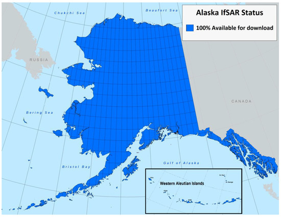
Figure 1.
Availability of IfSAR elevation data for Alaska as of June 2021 (Credit: Tracy Fuller, USGS. Public domain).
Over the past decade or so, increased availability of precise terrain data in the form of digital elevation models (DEMs) has led to improved hydrologic modelling and methods to extract more detailed and accurate watershed boundaries and stream networks [11,12,13,14,15,16,17]. The extraction of hydrographic features by modeling flow accumulation with a high-resolution (1–5 m cell size) DEM entails several challenges that require expert knowledge and techniques in several steps such as parameterizing extraction thresholds, eliminating flow obstructions, identifying headwater locations, interpreting image data for validation, and interactive editing of channels. These tasks are costly, involving tedious human interaction and judgment, which inevitably includes inaccuracies caused by inconsistent application of techniques over time and across space.
Application of machine learning techniques, such as artificial neural networks, that are well-trained to identify feature patterns or mimic complex feature interactions is an attractive alternative that could furnish more accurate results through more consistently applied workflows over time and space. Recent work with machine learning has revealed promising results for extraction of hydrography [18,19,20,21,22,23] and other associated features [24,25,26] from lidar point cloud and other remotely sensed data. Research presented in this paper aims to test and develop machine learning workflows to extract hydrographic features from 3DEP and other data to enhance the collection and validation of hydrography data.
Specifically, in this work, we test the capability of the U-net fully convolutional neural network (CNN) model to extract hydrographic waterbody polygons and drainage lines in Alaska using IfSAR-derived elevation and intensity data. The U-net deep learning model was originally applied to segmentation of electron microscopic images to track cells for biomedical research [27] but has since been applied to extraction of geospatial features, such as roads [28] and waterbodies [29]. The work presented here capitalizes upon the IfSAR digital models by generating elevation-derived layers—such as, curvature, topographic position index, and geomorphons—that have been shown to reflect geomorphic conditions [12,30,31,32]. Earlier work tested various iterations and parameters using object-based image analysis software to estimate the suitability of each layer for delineating waterbodies and streams [25,26,33]. The raster maps, or themes, found suitable are used as input data for U-net models. Reference hydrographic data, compiled to 1:24,000-scale (24k) specifications, are used for training and testing in this study. The U-net architecture was optimized through testing of sample size, window size, and sample augmentation. Probability values predicted by the U-net model are subsequently used as weights to inform flow-accumulation models for extraction of a complete vector drainage network.
Terrain analysis and digital modeling for estimating flow path and surface water depth are well traversed subjects [11,12,13,14,15,16,17,34]. Yet there is limited research on supervised extraction of all surface water features, including the elusive headwater features. Some research has been done in the extraction of hydrography from lidar and optical data using artificial neural networks (ANNs) [18,22,25], and significant progress has been made in their application in other environmental domains [35]. Regarding the use of radar data in ANNs to map water, [36] use a W-net neural network with Sentinel-1 and Sentinel-2 data to map land cover including water, and [37] test a fully convolutional network (FCN) to map floods using radar data, but neither study used elevation in their models.
To the best of our knowledge, this research is the first to apply an ANN to extract hydrography from feature maps that estimate the 3-dimensional form of the terrain surface, 2-dimensional overland flow, and reflected radiation, which are all derived from radar elevation and intensity data. This work also introduces a novel use of the ANN results to weight flow accumulation and derive connected vector-formatted flow networks. This strategy has advantages over past parametric weighting strategies due to the ability of ANN to adapt to varied environments and produce fuzzy outputs [38]. Extensibility of the developed ANN is tested in this work as well. Various percentages of training area, from about 3 to 35 percent of the study area, are used to train ANN models, and then each model is used to predict on the remaining area. A HPC environment enables concurrent processing of model workflows. Results indicate an optimal proportion of training data are required to model the hydrography, beyond which substantial benefits are not evident. Findings indicate a potential significant reduction in cost and labor required to derive surface water features from remotely sensed data. These implications may also inform other land surface and remote sensing classification efforts.
2. Materials and Methods
2.1. Study Area and Data
The study area contains fifty 12-digit Hydrologic Unit (HU12) NHD watersheds in north central Alaska, north of the arctic circle, with an area over 4600 km2 (Figure 2). The area is in the Northwest Arctic Borough and the Kobuk River crosses it towards the southern end. The Kobuk River valley is a broad low relief wetland area with broad meandering channels, wetlands, and ponds. Relief increases dramatically north of the river valley. Elevation in the study area ranges from 32 m to 1880 m above sea level. Kobuk is the smallest village in the Northwest Arctic Borough, with a 2018 population of 155. It lies on the western edge of the study area within the Kobuk River valley and comprises most anthropogenic features in the area. The HU12 catchments, which range in area from 31 to 239 km2, are processed and tested individually as detailed in the following sections.
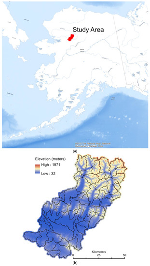
Figure 2.
(a) Location of study area in Alaska, and (b) study area covering fifty 12-digit Hydrologic Unit watersheds (black boundaries) in northcentral Alaska where elevation ranges from 32 to 1880 m above sea level.
2.1.1. IfSAR and Auxiliary Image Data
Source data used in this study are publicly available airborne IfSAR data that were collected between August 2012 and August 2013 [39,40,41,42]. The radar data are a combination of P- and X-bands with different frequencies required in different terrain conditions. For example, the X-band is optimal for glacier surfaces while the P-band is required for canopy penetration [43]. The RMSEz ranges from 0.55 m to 1.54 m across collected datasets.
3DEP distributes three primary products derived from the IfSAR data in Alaska: DSM, DTM, and orthorectified radar intensity images (ORI). The DSM estimates the elevation of the highest surfaces on the landscape which can include vegetation, built structures and the bare earth. The DTM represents a bare earth surface with vegetation and buildings removed. The DSM and DTM are provided with a 5-m spatial resolution. The ORI are radar backscatter intensity images and are available with a spatial resolution of 2.5 m or better depending on the collection. ORI resolution within the study area is 0.625 m. IfSAR products are hydro-flattened by collection contractors using radar response characteristics and visual inspection. In this process, waterbodies with an area greater than 8000 square meters are flattened to the elevation of the lowest bounding cell.
Satellite image data are used to review some areas where discrepancies exist between U-net predictions and reference hydrographic features. Alaska GeoNorth Information Systems provides Statewide Ortho Image web mapping services with panchromatic and color-infrared images at 1.5 m and 2.5 m resolution using best available image dates from SPOT satellites 5, 6, and 7 between 2010 and 2020. In addition, in October 2020, the USGS acquired 0.5-m resolution color-infrared Maxar satellite image data from 2010 and later, with most image data from January 2015 or later.
2.1.2. Reference Hydrography
Reference hydrographic features were compiled in vector format by USGS contractors in September of 2019 using the 2012–2013 IfSAR DTM and ORI data (Figure 3). The reference features are intended to represent stream center lines and polygonal waterbodies. The features were compiled to meet 24k USGS elevation-derived hydrography (EDH) specifications [44,45]. The hydrography derivation process applied a combination of routines based on flow direction and flow accumulation, geomorphon [46] and topographic openness information [47], and proprietary processing methods. SPOT image data guided manual editing of derived hydrographic features where needed. The derivation process is guided by the DTM and ORI data and thus the vector reference features are vertically and horizontally aligned with these data, making them a natural complement to the elevation data for the testing of hydrographic feature extraction from remotely sensed data. The resulting vertex spacing ranges from approximately 5 to 10 m, except for some artificial path features that represent flow paths through polygonal waterbodies. It should be noted that these reference data represent initial efforts to collect 24k hydrographic features from IfSAR.
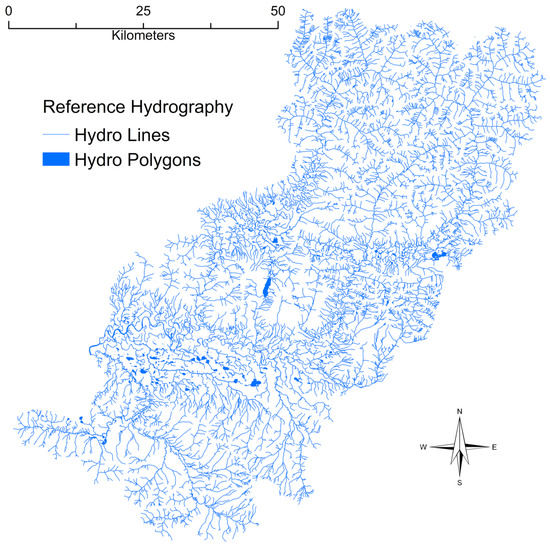
Figure 3.
Reference 1:24,000-scale hydrographic features derived from 2012–2013 IfSAR data through a contract to the U.S. Geological Survey in September 2019. The hydrography derivation used a combination of routines based on flow direction, flow accumulation, geomorphons, and topographic openness, along with proprietary processing methods.
Vector flowline features are buffered by 5 m to encapsulate related stream terrain features such as banks and bars. Resulting polygons and waterbody polygons are rasterized and used as reference water features to train and test the U-net ANN models.
2.2. Input Feature Layers
Fourteen co-registered raster layers are generated for each of the fifty HU12s in the study area (Table 1). All the layers, excluding the DSM and ORI, are derived from the filtered DTM and used as input layers for U-net model training and prediction. All layers are co-registered and clipped to the associated HU12 watershed boundary to ensure cells are aligned. Co-registration requires down-sampling of the ORI from 0.625-m to 5-m spatial resolution. A cubic convolution resampling process is applied to match cell resolution and co-register layers when necessary. All resulting input feature layers for each HU12 have 5-m resolution and the same raster size. The layers used are included because they have been found useful for delineating surface water features using multiscale object-based image analysis during this research or other studies suggest their utility for landform classification (see references in Table 1). The fourteen raster layers for HU12 190503021300 are shown in Figure 4. In preparation for modeling, all floating-point feature layers are normalized to unsigned integers to increase computational efficiency.

Table 1.
Source and description of layers used as inputs for the U-net model. DTM- Digital Terrain Model, DSM- Digital Surface Model, ORI- Orthorectified Radar Image, IfSAR- Interferometric Synthetic Aperture Radar.
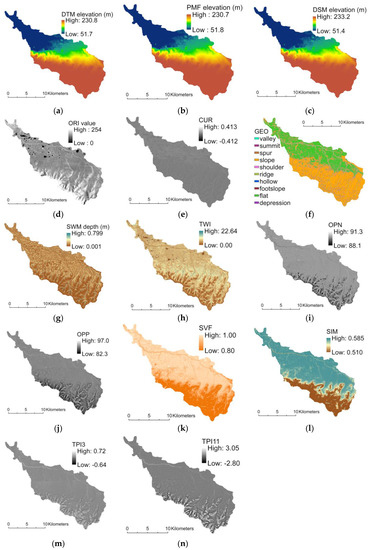
Figure 4.
Fourteen input feature layers for 12-digit Hydrologic Unit (HU12) watershed 190503021300 derived from interferometric synthetic aperture radar (IfSAR) data: (a) Digital Terrain Model (DTM), (b) Perona-Malik filtered (PMF) terrain model, (c) Digital Surface Model (DSM), (d) Orthorectified Intensity (ORI), (e) geometric curvature (CUR), (f) geomorphon (GEO) landscape type, (g) 2-D shallow water channel depth model (SWM), (h) topographic wetness index (TWI) (i) negative openness (OPN), (j) positive openness (OPP), (k) sky view factor (SVF), (l) sky illumination model (SIM), (m) topographic position index from 3 × 3 kernel (TPI3), and (n) topographic position index from 11 × 11 kernel (TPI11).
2.3. U-Net Model Architecture
This research expands the work of [33] and implements a U-net ANN architecture very similar to the model applied by [27], who also supply a graphic representation of the model. The U-net model is an FCN that avoids the use of dense connected layers, which reduces the number of tuning parameters and required computations compared to fully connected neural networks. The U-net follows an encoder-decoder architecture with contractive and expanding paths for feature segmentation. The contractive path applies six layers of two 3 × 3 convolutions with a 2 × 2 max pooling operation between each of the six convolutional layers. Pooling operations down-sample the feature maps generated by convolution layers and focus the important information in the layers.
In the expanding path, high-resolution information from the contractive path is combined with up-sampled feature maps to allow successive convolutions to learn to assemble more refined results. The expanding path has five layers of operations that include an up-sampling operation with concatenation of the corresponding-sized layer from the contractive path, followed by two 3 × 3 convolutions. Dropout is applied to the last up-sampled convolutional layer. Dropout randomly ignores some neuron activations’ samples to prevent strong correlation, which could lead to over training [54]. In our model, entire 2-dimensional feature maps are randomly dropped out (ignored) at a rate of 0.2 during each step of training.
Convolution layers are the primary computational environment within the FCN and serve to extract and filter information from images. Each convolution is batch normalized [55] and applies a rectified linear unit activation function to identify and preserve important feature characteristics and reduce redundancy and noise. The rectified linear unit activation function is a piecewise linear function that is commonly used in convolutional neural networks to truncate unimportant features and preserve important features [56].
A sigmoid activation function produces the final layer of the model. Weights are determined and adjusted during training using the “Adam” stochastic optimization algorithm [57] based on the Dice’s similarity coefficient [58]. The loss function that is minimized by the model is the negative of the Dice’s coefficient, which is a simple reproducible accuracy measure found useful for image segmentation [59]. Additional details and optimization of the U-net model for hydrography extraction are documented by [33]. Model training continues for 50 epochs because learning rates appear to plateau around this number of epochs.
Selection of Training Samples
The patch size, or analytical window size, used here is 224 × 224 cells, which is less than half the 572 × 572 patch size used by [27]. The patch size is an important parameter because the larger the patch the larger the computational burden, whereas if a patch is too small relevant patterns for feature extraction may be missed. Thus, the patch size has a large bearing on model accuracy and efficiency. Applying a U-net model on similar feature maps derived from 1 m lidar elevation and intensity data, [33] determined a 224 × 224 patch size is effective for extracting hydrographic features. An analytical window of the patch size (224 × 224 cells) is called a sample. Here 400 samples are randomly selected from a HU12 with 200 samples centered on non-water cells and 200 centered on water cells as identified by the rasterized training data. One of every four samples is randomly selected and augmented using one mirror, two rotation, two rescaling and one shear operations. The augmentation process generates six additional samples for every four samples yielding a total of 1000 samples for training each HU12, 400 original samples and 600 augmented samples. During model building, two-thirds of the 1000 samples are used for training and one-third are used for validation. Sample windows are extracted for all input raster feature layers and the raster reference layer.
2.4. HPC Processing Environment
The U-net model is implemented using Python, Keras and Tensorflow tools. The HPC platform consists of a 12-node Linux cluster running Centos 7.0, with 20 Xeon E5-2650 (2.3 GHz) processing cores and 128 Gigabytes of random-access memory (RAM) on each node. Files are stored through a single NFS share consisting of 12 drives in a redundant array of disks. Quad fourteen data rate (FDR) InfiniBand interconnects support up to 54 Gigabit per second data transfer rates. Resource allocation and job processing are managed through Slurm Workload Manager. A single model was trained on each processing node, which allowed up to 12 models to be trained simultaneously on the 12-node Linux cluster.
2.5. Design for Extensibility
To estimate model extensibility, sixteen U-net models are trained and tested for the fifty HU12 study area. The sixteen models are trained with an increasing number of HU12 watersheds, which are assigned an order from 1 to 16. Models are numbered from one to sixteen and include all watersheds with an order that is equal to or less than the model number (Figure 5). For example, model five is trained with watersheds ordered one through five. Training watersheds are arranged to be evenly distributed over the study area for each model. The area of the training watersheds ranges from 50 to 188 km2. Based on the sum of the area of the training watersheds, the proportion of the total study area used for training the 16 models ranges from 0.02 to 0.34 for models 1 through 16, respectively, which is about 2 percent of the study area per training watershed. Predictions are generated from each of the sixteen models for all fifty watersheds in the study area.
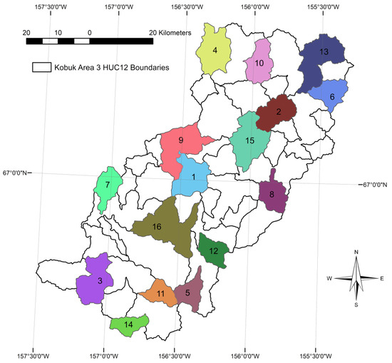
Figure 5.
Distribution and order number of the sixteen selected 12-digit Hydrologic Unit (HU12) watersheds in the fifty-HU12 study area that are used for training the sixteen U-net models, numbered 1 through 16. Numbers on the watersheds indicate the order used to add each HU12 watershed for training a model. Model numbers are trained with all watersheds having the order number that is equal to or less than the model number. Thus, model 1 is trained with HU12 #1, and model 2 is trained with HU12s #1 and #2, and so forth to model 16, which includes HU12s #1 through #16.
2.6. Accuracy Metrics
A trained U-net model predicts the likelihood (or probability), ranging from 0 to 1, that the cells in a watershed represent surface water, and it is applied to all fifty watersheds in the study area. Scores of 0.5 and higher are considered positive predictions for water. The U-net model minimizes the loss function, which is the negative of Dice’s coefficient for this research. Equation (1) shows the calculation for Dice’s coefficient. A true positive (TP) pixel is a pixel predicted as water that is water in the reference. A true negative (TN) is a predicted non-water pixel that is non-water in the reference. Whereas a false positive (FP) pixel is predicted water that is non-water in the reference, and false negative (FN) pixel is predicted non-water that is water in the reference. Note that model accuracy (Equation (2)) is not used here because a vast majority of feature content is non-water features, or TN values, which consistently generates high accuracy values with low sensitivity to model changes. During model development learning is regulated over each epoch for training and validation samples through the loss function. Dice values from the last epoch are evaluated to compare model performance with increasing training data.
Precision, recall, and F1-score are determined for each training watershed for each model. Precision (Equation (3)) is the percent of predicted pixels correctly labeled. Recall (Equation (4)) is the percent of reference pixels correctly labeled. F1-Score is a quality score that combines precision and recall [60]. It should be noted that F1-score and Dice’s coefficient are identical computations. Model solutions are also used to predict water features (pixels) for all HU12 watersheds that are not used for training. These are referred to as test watersheds and the number of test watersheds ranges from 49 to 34 for models 1 through 16, respectively. Average precision, recall, and F1-scores are computed for these training watersheds and for test watershed for each model.
Dice’s coefficient = 2TP/(2TP + FP + FN)
Accuracy = (TP + TN)/(TP + TN + FP + FN)
Precision = TP/(TP + FP)
Recall = TP/(TP + FN)
F1-score = 2(Precision × Recall)/(Precision + Recall)
In addition, to determine if elevation or relief affect U-net predictions, elevation statistics (mean, standard deviation, minimum, maximum, and range) are computed for each HU12 and compared with U-net model F1-scores.
2.7. Significance of Layers
To determine how much each of the input feature layers influences the U-net hydrography extraction model, the contribution of each layer to a trained model is estimated using an iterative randomization process. The mean squared error (MSE), as shown in Equation (6), is the error estimate used to compare models:
where is the reference value and is the associated predicted value.
The contribution of a layer in a trained model is estimated by substituting a layer of random values for the layer being tested and then recomputing predictions, MSE, and F1-score for the trained model using the randomized layer. If a layer significantly contributes to the model, the MSE with the randomized layer will be greater than the original MSE.
Measures are only determined for the model that is trained with 14 HU12 watersheds (i.e., model 14) because this model is more effective than other models that use less training data. Each of the 14 input layers is randomized ten times. As shown in Equation (7), the average error difference for a test layer is computed as the average of ten MSEs (average MSEl) determined from ten randomizations of the test layer minus the MSE of the original model without any randomizations. The percent that each layer contributes to a model is estimated as the average error difference for that layer divided by the sum of the average error differences for each of the 14 layers in the model. Average and standard deviation of the layer percent contributions are determined for the watersheds used to train model 14.
In addition, the layer randomization process is used to measure how much a layer contributes to a model based on the change in F1-scores. In general, if a layer helps improve a model, randomizing the layer reduces the F1-score for a model. The average and standard deviation of the percent that the original non-randomized F1-score is reduced by the randomization of a layer is computed for the 14 training watersheds.
2.8. Weighted Flow Accumulation Network Extraction
This section describes the novel use of ANN predicted probabilities as weights in the flow accumulation process to constrain extracted drainage networks to follow ANN predictions, and thereby generate a connected drainage network. U-net model results provide a raster layer of water and non-water pixels. In order to vectorize U-net predictions, the U-net probability raster layer is used to guide elevation-derived flow accumulation. The workflow to extract a vector drainage network from a U-net-guided flow accumulation includes DTM conditioning through pit filling, D-8 flow-direction routing, weighted D-8 flow accumulation, and drainage channel extraction, which is implemented with the Terrain analysis using Digital Elevation Model (TauDEM) tools (https://hydrology.usu.edu/taudem/taudem5/, accessed on 3 June 2021). [61] describe a similar workflow for generating a weighted flow accumulation (WFA) raster but their weights are based on local curvature. Here we use the U-net probability raster to weight flow accumulation. U-net predicted probabilities are zero everywhere except within predicted drainage channels and waterbodies. Consequently, flow accumulation is set to zero everywhere except within U-net predicted water cells, and extracted drainage lines are forced to follow U-net predictions.
Using this method, WFA drainage networks are extracted from the DTM for each HU12 watershed in the study area. This process is demonstrated using U-net probabilities predicted from model 14, which uses 14 HU12 watersheds for training data. In this workflow, flow accumulation thresholds for network extraction are iteratively determined to extract about the same length of flowlines that exist in the 24k reference hydrographic features for each watershed. After extraction, the drainage networks are rasterized with a 5 m buffer and these pixels are added to the U-net predictions to form connected channels in the U-net predictions. Subsequently, accuracy metrics are generated for these augmented predictions and compared to the original U-net predictions.
3. Results and Discussion
3.1. Model Training
The minimum time required to train the U-net model using a single processing node (includes 20 Xeon E5-2650 processing cores and 128 Gigabytes of RAM) of the Linux cluster was about five hours to train model 1, which was trained with a single watershed. While continuing to train one model per processing node, about two additional hours were required for training for each additional watershed included in a model. Model 16, with 16 training watersheds, required about 33 h for training. The HPC environment allowed simultaneous processing of the sixteen test models, which generated results about four times faster than sequential processing.
Validation loss curves for the 16 models indicate that a stable plateau for validation scores is achieved around 30 to 50 epochs when four or more training watersheds are included in the models (Figure 6). However, an outlying observation appears (as a spike) at about 40 epochs in the validation scores for the model with eight training watersheds, and similar spikes are apparent for other models with fewer training watershed. Such spikes could indicate some instability in model predictions or sample data anomalies occurring in the batch normalization process. No outlying validation observations are apparent in validation loss curves for models with nine or more models. Although training loss curves suggest additional accuracy could be achieved by training beyond 50 epochs, validation curves for models with more training data (13 to 16 watersheds) indicate little, if any, improvement could be achieved by extending training epochs.
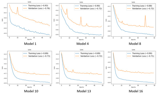
Figure 6.
Training and validation loss for six models using increasing training data. Models 1, 4, 8, 10, 13, and 16 use 1, 4, 8, 10, 13, and 16 12-digit hydrologic unit (HU12) watersheds for training, with 1000 samples used for each watershed.
Stable training accuracies with Dice coefficients ranging from 0.88 to 0.90 are achieved for models with seven or more training watersheds (Figure 7). Dice values range from 0.70 to 0.74 for validation samples for models with seven or more training watersheds. Dice scores appear slightly more stable for models with 13 to 16 training watersheds, when training scores range from 0.89 to 0.90 and validation scores range from 0.71 to 0.72. While using a similar U-net model to predict hydrographic streams from lidar data, [33] reports 13 percent difference between training and validation samples, achieving Dice values of 0.97 and 0.84 for training and validation, respectively.
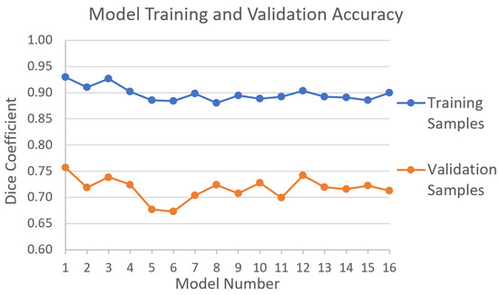
Figure 7.
Training and validation accuracy for sixteen models using increasing training data. Models 1 to 16 use 1 to 16 12-digit hydrologic unit (HU12) watersheds for training, respectively, with 1000 samples selected in each watershed.
3.2. Model Test Results
Accuracy metrics from U-net model predictions for training watersheds are shown in Figure 8. Average precision values range from 83 to 94 percent and are consistently higher than recall values by 7 to 24 percent. This indicates U-net predicted hydro water pixels are very likely in the reference water pixels, however, not enough water pixels are being predicted by the models. That is, a larger proportion of false negative predictions are made by the U-net models than false positives. Average F1-scores for the training watersheds range from 75 to 90. Yet more consistent precision, recall, and F1-score values result when seven or more watersheds are used for training when average F1-scores range from 80 to 82. As seen in Figure 8b, adding training watersheds continues to improve U-net predictions for watersheds 1 through 4 until seven watersheds are used for training in model 7. The seven watersheds are about 15 percent of the study area. Additional training beyond seven watersheds does not improve predictions (Figure 8).
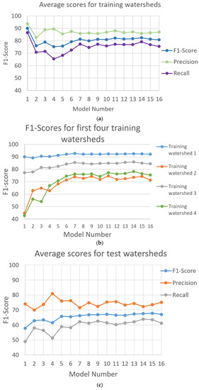
Figure 8.
Average accuracy values of precision, recall, and F1-score for (a) training watersheds and (c) test watersheds in the 50-watershed study area in Alaska determined from hydrographic feature predictions from 16 U-net models that use an increasing number of training watersheds. (Note: Model 1 was trained with watershed 1, model 2 was trained with watersheds 1 and 2, and model 3 was trained with watersheds 1, 2, and 3, and so forth to model 16). Model 1 averages are the accuracy values for training watershed 1, and model 2 averages are determined from accuracy values for training watersheds 1 and 2, and so forth to model 16 that shows averages for all 16 training watersheds. Panel (b) shows average values for the first four training watersheds. Averages for test watersheds (c) are determined from the 49 to 34 watersheds that are not used for training models 1 to 16, respectively. Reference features are rasterized 1:24,000-scale hydrographic features derived from 2012–2013 IfSAR data through work contracted by the U.S. Geological Survey in September 2019.
Figure 8c shows average accuracy metrics for U-net predictions for the test watersheds. Average precision values range from 70 to 81 for test watersheds. As was seen for training values, average recall values, ranging from 49 to 64 percent, are consistently lower than average precisions by 8 to 30 percent. So again, a larger proportion of false negatives are predicted than false positives by U-net models for test watersheds. Average F1-scores for test watersheds range from 58 to 68 percent. F1-scores for test watersheds also improve by increasing the number of training watersheds up to seven, when F1-scores range from 66 to 68.
Overall, average metrics summarizing predictions for test watersheds are between 9 and 38 percent lower than associated values for training watersheds. F1-scores for test watersheds average about 14 percent lower than F1-scores for test watersheds when sufficient training data are used (i.e., training with seven or more watersheds). This is consistent with the differences seen between training and validation samples during model training (Figure 7). Whereas predictions may be slightly (perhaps one or two percent) improved by extending training for additional epochs, evidence suggests little can be gained by including additional training data beyond seven watersheds (about 15 percent of the study area) for tested U-net models using 5-m IfSAR data.
3.2.1. Model Waterbody Tests
This section compares vectorized representations of U-net predicted water polygons to reference water polygons. Comparisons are demonstrated only for model 14 predictions, which is trained with 14 HU12 watersheds. Figure 9 shows resulting accuracy scores for model 14 vectorized water polygons with relation to the total area of water polygons in each watershed. Precision and recall values for training watersheds range from 94 to 99 percent, and 35 to 99 percent, respectively, resulting in F1-scores that range from 51 to 99 percent and average 93 percent. Precision, recall, and F1-scores for test watersheds range from 0 to 99 percent, 0 to 99 percent, and 0 to 98 percent, respectively, with F1-scores averaging 77 percent. Figure 9 indicates the watersheds with less waterbody content have lower accuracy values.
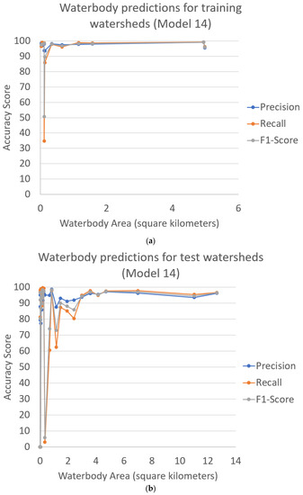
Figure 9.
Accuracy scores (precision, recall, and F1-score) for predictions of waterbody features for (a) the 14 training HU12 watersheds and (b) the 36 test HU12 watersheds compared to total waterbody polygon area in reference hydrography. Predictions are determined from U-net model 14 using 14 HU12 training watersheds.
One training watershed and five test watersheds have very low F1-scores between 0 and 50 percent. All of these watersheds have very few detailed waterbodies that are either not in the predicted polygons or not in the reference polygons, which generate low F1-scores. The process of vectorizing raster water pixels to waterbody polygons converts contiguous groups of predicted water pixels (i.e., clumps) to polygonal waterbodies but is constrained to minimum area and widths of predicted pixel clumps. This means some predicted waterbody pixels that are part of a clump may not be converted to polygon waterbodies, which causes some low recall scores. Such a case is demonstrated in Figure 10 for training watershed 4, where only portions of a narrow stream are converted to waterbody polygons, and the rest of the stream is included in predicted water pixels. Generally, extraction of waterbody polygons from the U-net predictions is highly accurate for watersheds with larger waterbodies, but poor results are found for watersheds with few finely detailed waterbodies.
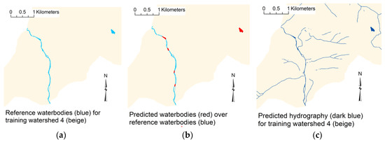
Figure 10.
(a) Reference hydrography, (b) waterbodies extracted from predictions (red) displayed over reference waterbodies, and (c) predicted hydrography pixels from model 14 for a section of reference HU12 watershed 4 (190503021004).
To further explore the effect of the distribution of details in hydrographic features on model predictions, F1-scores are compared to the ratio of the total area of waterbody polygons to the total length of flowline features in each watershed, where ratios are determined from the reference hydrography. As seen in Figure 11, the ratio of area-feature content to line-feature content (area-to-line ratio) is positively correlated with F1-scores, having polynomial relations with R2 values of 0.5 and 0.7, for training and test watersheds, respectively. Considering that linear flowline features require more detail to map than larger waterbody features, the area-to-line ratio is an inverse indicator of the relative level of detail, or mapping complexity, for the U-net hydrographic models. That is, a watershed with a low area-to-line ratio is more complex to map with a U-net model than a watershed with a high area-to-line ratio. This result can help guide the sample selection for model training. For instance, training watersheds should be selected that span the full range of hydrography complexity as estimated by the area-to-line ratio. Our set of training watersheds could be improved in this manner because it only spans about half of the area-to-line ratio values in the study area (Figure 11). Additionally, the area-to-line ratio could be used to ensure training windows are distributed over the range of complexities within a watershed.
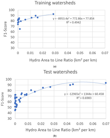
Figure 11.
Comparison of F1-scores from model 14 with the ratio of the total area of waterbody features to the total length of flowline features for (a) training watersheds and (b) test watersheds. Waterbody area and flowline length are determined from the reference hydrography. Polynomial relations for training and test watersheds have R2 values of 0.49 and 0.70, respectively.
3.2.2. Spatial Relations of Model Results
The spatial distribution of average F1-scores for the U-net model 14 (trained with 14 watersheds) is shown in Figure 12 alongside average elevations of the watersheds in the study area. No spatial relation is evident between F1-scores and average elevation as depicted in Figure 12. No linear relation is evident between F1-scores from model 14 and summary statistics (mean, standard deviation, and range) for elevation for the 36 test watersheds (Figure 13). Thus, no obvious reason for variations in F1-scores is caused by elevation. It has been reported that IfSAR elevation accuracy is reduced with increasing slope [62,63] and with increasing forest canopy [64]. Yet, no relation between hydrography prediction accuracy and terrain conditions are found in these results. This suggests the U-net model is sufficiently trained to account for variations in terrain conditions, which is expected given that input layers are derived from the IfSAR terrain data to describe numerous aspects of the terrain.
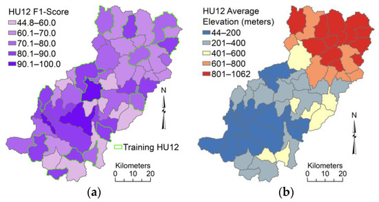
Figure 12.
Spatial distribution of (a) F1-scores for HU12 watersheds for hydrography predictions from U-net model using 14 HU12 watersheds for training (green boundaries), and (b) of average elevation values for each HU12 watershed in the 50 HU12 study area.
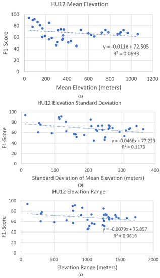
Figure 13.
Plot of linear relations between (a) mean, (b) standard deviation, and (c) range in elevation for HU12 watersheds and F1-scores determined for 36 test HU12 watersheds. Hydro features are predicted from the U-net model 14 trained with 14 HU12 watersheds.
3.2.3. Review of Reference Hydrography
Results indicate about 80 percent accurate hydrography predictions can be achieved by training all watersheds in a project area, and about 70 percent accuracy can be achieved by training with 15 percent or more of an area. Using a similar model with high-precision Geiger-mode lidar data and derived layers at 1-m resolution for a watershed in North Carolina, [33] predicted hydrography that achieved F1-scores from test areas between 81 and 92 percent. Compared to [33] results, our F1-scores are 10 to 20 percent lower. Several reasons why our F1 results are lower than [33] study are because our study uses lower resolution data, is applied to a much larger area with a wider range of terrain and environment conditions, and uses a different sampling strategy and a different U-net model (i.e., spatially larger training window, fewer training epochs, fewer training samples, and fewer convolutional layers). Results achieved in our study may be acceptable for validating or guiding newly collected hydrography data but are not adequate for acquiring new hydrography to update national databases.
The accuracy of the reference data can have a major influence over the quality of neural network predictions [65]. So, it is crucial to verify the quality of reference features. Figure 14 compares a low-relief section of reference hydrography around the Kobuk River with orthorectified 0.5 m color and 2.5 m color-infrared satellite image data. Exact image acquisition times are not available, but best available images are used that are within a few years of the reference hydrography collection. Some difference in wetness conditions between images and reference data may exist because of different acquisitions times. Red boxes in panel c of Figure 14 show areas in the color image where reference hydrography appears to be missing waterbody or stream polygons. Dark areas in the color-infrared image (panel d) corroborates that these features are missing in the reference hydrography. In addition, model 14 predictions, shown in panel e, include water pixels at the locations of some of these missing reference polygons. The center red rectangle of panel e shows where a predicted flowline does not follow the reference flowline.
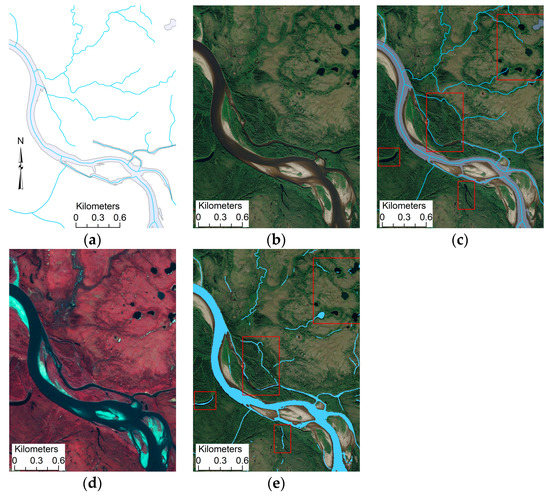
Figure 14.
Shown for a low-relief area near the Kobuk River are (a) reference hydrography, (b) 0.5-m resolution color images from Maxar satellite, (c) reference hydrography over 0.5-m Maxar image, (d) 2.5-m color-infrared SPOT image, and (e) U-net predictions (sky blue) from model 14 over the 0.5-m resolution Maxar image. Red rectangles highlight areas in c where reference hydrography appears not well integrated with satellite information and areas in e where predictions deviate from reference hydrography but may better integrate with satellite images.
The southwest area including the lower three boxes in Figure 14 are from a test watershed with a 91 percent F1-score, and the northeast section is from a watershed with 46 percent F1-score. In the northeast section, it is evident from the images that several smaller waterbodies are not included in predictions nor in reference hydrography, which is largely caused by minimum size constraints for waterbody collection. In comparison to reference features, flowline features also are not predicted well in the northeast section, with poor connectivity in the predicted network.
Overall, the various types of discrepancies between the reference hydrography and image information, which are influenced by collection standards, suggest inaccuracies in the reference hydrography are influencing resulting U-net prediction accuracies. Additional effort is needed to ensure the quality of reference hydrography to improve model predictions.
3.3. Significance of Model Layers
Initial results from layer significance testing are shown in Figure 15. Based on average change in MSE values for 10 randomizations of each layer, the shallow water model (SWM), digital surface model (DSM), and positive openness (OPP) respectively contribute about 71, 8, and 4 percent, which accounts for about 83 percent of the model error in training watersheds. Likewise, SWM, DSM, and OPP respectively account for about 75, 9, and 4 percent of the model error for test watersheds, totaling 88 percent. For the lowest contributions, Perona-Malik filtered terrain model (PMF), topographic position index from 3 × 3 window (TPI3), and curvature (CUR) account for less than 3 percent of the model error for training watersheds, and less than 1 percent of model error for test watersheds. Given that all the layers, other than DTM, DSM, and ORI are derived from the PMF layer, it is expected that most information in the PMF layer is included in the other layers, and it may be possible to exclude this layer from models for processing efficiency.
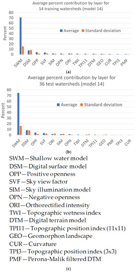
Figure 15.
Average percent contribution of each input layer for U-net model 14 that uses 14 watersheds for training. Contribution for a layer is estimated from the average change in 10 model mean squared error values (MSE) from the original model MSE based on 10 separate randomizations of an input layer. Average contributions for input layers in (a) the 14 training watersheds, and (b) the 36 test watersheds, with layer names shown in (c).
Average change in F1-scores for original model 14 as estimated by 10 separate randomizations of a layer are shown in Figure 16. Average changes range from 20 to 93 percent for training watersheds, and from 10 to 91 percent for test watersheds. The three layers causing the greatest change in F1-scores with randomization are SWM, sky illumination model (SIM), and OPP for both the training and test watersheds. Whereas PMF, TPI3, DTM, and geomorphon (GEO) cause the least change in F1-scores for training and test watersheds. Computation of MSE values includes the true negative values (true non-water predictions), which involves a vast majority of predicted pixels, whereas true negatives are excluded from F1-scores. Therefore, the change in F1-scores may be a more useful metric for assessing the layer contributions to models than change in MSE. However, additional normalizations may be needed to form more precise average estimates because standard deviations of average changes in F1-scores are large (greater than 50 percent) compared to average values for 9 of 14 input layers based on test watersheds (Figure 16b).
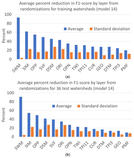
Figure 16.
Average percent reduction in F1-score of each input layer for U-net model 14 that uses 14 watersheds for training. Percent reduction for a layer is estimated from the average change in F1-scores from the original model determined from 10 models that separately randomize the layer 10 times. Average and standard deviation of F1-score reductions for input layers in (a) the 14 training watersheds, and (b) the 36 test watersheds.
3.4. Flow Accumulation Network Extraction
U-net predictions for model 14 that are augmented with drainage network pixels extracted with the D-8 flow accumulation model weighted by U-net probabilities form more connectivity in the predictions, but do not improve F1-scores. Accuracy values for training watersheds with and without flow-network augmented predictions from model 14 are shown in Figure 17. Precision, recall, and F1-scores from network-augmented predictions for the 14 training watersheds respectively average 65, 84, and 73 percent, versus corresponding averages of 86, 79, and 82 percent without augmentation (Table 2). The additional water pixels from network augmentation reduce false negatives thereby increasing recall scores, but more often they increase false positives, which decreases precision scores, leading to lower F1-scores.
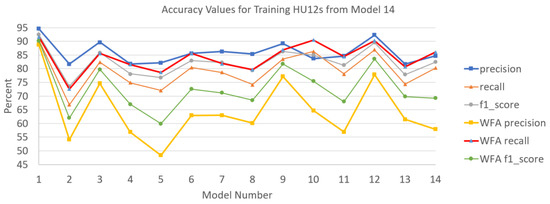
Figure 17.
Accuracy values for the 14 training watersheds used in U-net model 14 compared to corresponding values resulting from U-net model 14 augmented with flow network features extracted from a D-8 flow accumulation model weighted with model 14 probabilities.
Table 2.
Summary statistics for precision, and F1-scores resulting from predictions for the 14 training and 36 test watersheds using U-net model 14 with comparison to corresponding values predicted from U-net model 14 augmented with flow network features extracted from a D-8 flow accumulation model weighted with model 14 probabilities.
As seen in Table 2, network-augmented predictions for the 36 test watersheds average 56, 72, and 63 percent for precision, recall, and F1-score, respectively. Corresponding precision, recall, and F1-scores from predictions without augmentation average 72, 64, and 68 percent, respectively. Again, network augmentation generates lower precision but higher recall values leading to a 5-percent lower average F1-score for test watersheds, which is about half of the average F1-score difference seen for training watersheds.
Figure 18 demonstrates the improved connectivity generated by augmenting predictions with flow network features from the WFA models. The additional network features extracted with WFA models and constrained by U-net probabilities form much better network connectivity among predicted features than without this augmentation, as clearly seen in the red boxes in Figure 18b,c. However, the additional network predictions do not always follow network features in the reference hydrography, as shown in red boxes of Figure 18d. Further testing of this network extraction process is ongoing to determine any limitations in complex drainage areas, such as in low relief braided stream areas where divergent flow paths can exist. Alternative flow-routing approaches, such as D-infinity [66] or least-cost path [17,67], may provide better networks for augmentation than the D-8 method.
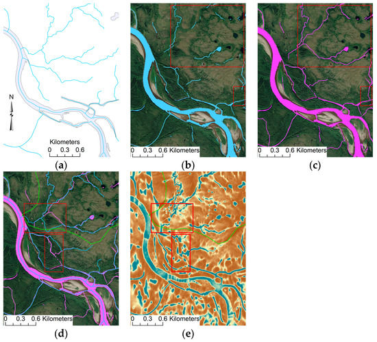
Figure 18.
Comparison of (a) reference hydrography with (b) U-net model 14 predictions (c) U-net model 14 predictions augmented with flow network extracted with the D-8 flow accumulation model weighted with model 14 probabilities, (d) augmented model 14 predictions with reference flowline network, and (e) 2-D shallow water depth model with deep channels in darker blues and higher terrain in darker browns. Red boxes highlight areas for discussion, and the green line in d and e is a watershed boundary.
In comparison to the most influential layer in the U-net model, the 2-D SWM that estimates channel depth (Figure 18e), the reference hydrography and the U-net predictions both tend to follow deep channel paths but sometimes take alternative paths, which creates lower precision scores in the augmented predictions. The 2-D shallow-water model uses Green’s function stochastic method [50,68] to solve the bivariate form of Saint-Venant Equations, which is a solution based on the concept of duality between the field and particle representation for overland flow.
Aside from the DTM, inputs to the SWM include a flow gradient vector, rainfall excess rate (200 mm/hour), Manning’s roughness coefficient (0.05), a diffusion coefficient (6.0), and a water depth threshold (2.0 m). Parameter values used here are shown in parentheses. The flow-gradient vector is determined by first-order partial derivatives in x and y from the DTM. Further work is needed to test alternative solutions for the SWM by varying input parameters to the SWM, and applying a flow-direction raster, such as D-infinity, to generate the partial derivative inputs [69]. Also, the error map from the SWM can be used as an additional layer in U-net models, which may force predictions to follow more accurate channels in the SWM.
4. Summary and Recommendations
Accurate hydrographic feature data that are integrated with high-resolution elevation data are critical for hydrologic investigations and for management and planning activities of water and other natural resources. This paper evaluates the use of machine learning for automated extraction of hydrographic features from USGS 3DEP IfSAR elevation data for a 50-watershed study area in northern Alaska. A series of U-net neural network models with increasing levels of training are evaluated. This novel implementation of the U-net model uses 3-D terrain attributes, 2-D flow, and reflected intensity information, all derived from radar data, to predict hydrography. The work also demonstrates how associated vector drainage networks can be generated through a U-net weighted flow accumulation model to augment model predictions. The research indicates the U-net neural network provides a viable solution for automated extraction of hydrography from 5-m resolution IfSAR elevation and intensity data in northern Alaska that can aid validation and improvement of 24k hydrography data. Using 24k NHD hydrography as reference data for training and testing, about 80 percent accurate hydrography predictions can be achieved by training all watersheds in a project area, and about 70 percent accuracy can be achieved by training with 15 percent or more of an area. Results indicate there is an optimal proportion of training data (about 15 percent of the study area) required to model hydrography, beyond which substantial benefits are not seen. These findings indicate a potential significant reduction in cost and labor required to derive surface water features from remotely sensed data.
A summary of the key findings follows:
- Hydrography prediction accuracies averaging near 70 percent can be achieved by training the described U-net model with about 15 percent of the project area using reference data having the same quality as what is used in this study. Little can be gained by including additional training data beyond 15 percent of the study area.
- Evaluation of predicted waterbodies provides F1-scores that average 77 percent for tested watersheds. Accuracies are positively correlated with the area-to-line ratio of hydrography content in the watersheds. That is, U-net waterbody predictions are highly accurate for watersheds with larger waterbodies, but less accurate for watersheds comprised mostly of finely detailed waterbodies and drainage channels.
- Precision values are 7 to 30 percent higher than recall values, which indicates predicted water pixels are likely to be included within reference water pixels, however not enough water pixels are being predicted by the models.
- Layer significance testing indicates the SWM layer contributes the largest amount of information to the U-net model predictions, averaging 71 to 93 percent, which is more than 20 percent higher than the next most influential layer.
- Augmenting U-net predictions with D-8 flow accumulation network features improves connectivity that increases recall but more so decreases precision, leading to F1-scores averaging 63 percent, which is about 5 percent less than predictions without augmentation. Comparisons with satellite image data and the most influential layer, SWM, indicate predicted flow paths and reference hydrography both follow probable flow paths, but sometimes take alternate routes.
Further work is needed to improve predictions to a level that will support subsequent collection of hydrographic features. Aside from excluding the PMF layer from models, recommendations for model improvement include:
- (1)
- Better verification of reference hydrography data, or use of hydrographic features compiled at a higher level of detail than 24k,
- (2)
- Eliminating uncertain reference features from training data, and ensuring training windows include minimum overlap and are sufficiently distributed over the range of conditions with consideration to area-to-line ratios of hydrographic feature content, and
- (3)
- Continuation of model training until a learning rate plateau is achieved.
The SWM appears to be the most influential layer in U-net models for this Alaska study area. Subsequent work will evaluate alternative SWM solutions and test other promising U-net options for other areas in Alaska, such as removing the PMF layer, adding a layer for SWM error, and adding satellite image information. In addition, alternate flow-routing methods to extract drainage networks from U-net predictions, such as D-infinity or least-cost path, will be evaluated.
Author Contributions
Conceptualization, L.V.S., E.J.S., S.W. and Z.J.; methodology, L.V.S., E.J.S., S.W. and Z.J.; project administration, E.J.S., S.W. and E.L.U.; software, E.M., L.V.S., A.D. and J.S.; validation, L.V.S., E.J.S., E.M., A.D. and J.S.; formal analysis, L.V.S., E.M., A.D. and J.S.; investigation, L.V.S., E.J.S.; data curation, L.V.S. and E.M.; writing—original draft preparation, L.V.S. and E.J.S.; writing—review and editing, L.V.S., E.J.S., S.W., Z.J., E.J.S., E.L.U., E.M. and A.D.; visualization, L.V.S. All authors have read and agreed to the published version of the manuscript.
Funding
This paper and associated materials are based in part upon work supported by the National Science Foundation (NSF) under grant numbers: 1743184, 1850546, and 2008973. Any opinions, findings, and conclusions or recommendations expressed in these materials are those of the authors and do not necessarily reflect the views of NSF. This article has been peer reviewed and approved for publication consistent with USGS Fundamental Science Practices (https://pubs.usgs.gov/circ/1367/).
Data Availability Statement
Source data used in this study are publicly available airborne IfSAR data that were collected between August 2012 and August 2013 (USGS, 2017a, https://www.sciencebase.gov/catalog/item/5641fe98e4b0831b7d62e758; USGS, 2017b, https://www.sciencebase.gov/catalog/item/543e6a6ae4b0fd76af69cf47; USGS, 2017c, https://www.sciencebase.gov/catalog/item/543e6acde4b0fd76af69cf4a; USGS 2021, https://apps.nationalmap.gov/). Reference hydrographic data has been included in the National Hydrogaphy Dataset and can downloaded from the National Map download page (https://apps.nationalmap.gov/downloader/#/).
Acknowledgments
The authors would like to thank USGS research scientist, Sam Arundel, for a thorough review of this article, USGS National Geospatial Technical Operations staff, including Silvia Terziotti, and Christy-Ann Archuleta for details about the most current hydrography in the study area, and the anonymous reviewers for their conscientious and thorough reviews of this article.
Conflicts of Interest
The authors declare no conflict of interest.
Disclaimer
Any use of trade, firm, or product names is for descriptive purposes only and does not imply endorsement by the U.S. Government.
References
- Maidment, D.R. Conceptual framework for the national flood interoperability experiment. J. Am. Water Resour. Assoc. 2016, 53, 245–257. [Google Scholar] [CrossRef]
- Chen, B.; Krajewski, W.; Goska, R.; Young, N. Using LiDAR surveys to document floods: A case study of the 2008 Iowa flood. J. Hydrol. 2017, 553, 338–349. [Google Scholar] [CrossRef]
- Regan, R.S.; Juracek, K.E.; Hay, L.E.; Markstrom, S.L.; Viger, R.J.; Driscoll, J.M.; Lafontaine, J.H.; Norton, P.A. The U.S. Geological Survey National Hydrologic Model infrastructure: Rationale, description, and application of a watershed-scale model for the conterminous United States. Environ. Model. Softw. 2019, 111, 192–203. [Google Scholar] [CrossRef]
- Simley, J.D.; Carswell, W.J., Jr. The National Map–Hydrography. U.S. Geological Survey Fact Sheet; 2009. Available online: http://pubs.usgs.gov/fs/2009/3054/ (accessed on 30 April 2020).
- Wright, W.; Nielsen, B.; Mullen, J.; Dowd, J. Agricultural groundwater policy during drought: A spatially differentiated approach for Flint River Basin. In Proceedings of the Agricultural and Applied Economics Association 2012 Annual Meeting, Seattle, WA, USA, 12–14 August 2012. [Google Scholar]
- Schultz, L.D.; Heck, M.P.; Hockman-Wert, D.; Allai, T.; Wenger, S.; Cook, N.A.; Dunham, J.B. Spatial and temporal variability in the effects of wildfire and drought on thermal habitat for a desert trout. J. Arid. Environ. 2017, 145, 60–68. [Google Scholar] [CrossRef]
- Poppenga, S.K.; Gesch, D.B.; Worstell, B.B. Hydrography change detection: The usefulness of surface channels derived from LiDAR DEMS for updating mapped hydrography. J. Am. Water Resour. Assoc. 2013, 49, 371–389. [Google Scholar] [CrossRef]
- Terziotti, S.; Adkins, K.; Aichele, S.; Anderson, R.; Archuleta, C. Testing the waters: Integrating hydrography and elevation in national hydrography mapping. AWRA Water Resour. IMPACT 2018, 20, 28–29. [Google Scholar]
- Maune, D.F. Digital Elevation Model (DEM) Data for the Alaska Statewide Digital Mapping Initiative (SDMI). Alaska DEM Workshop Whitepaper; 2008. Available online: http://agc.dnr.alaska.gov/documents/Alaska_SDMI_DEM_Whitepaper_Final.pdf (accessed on 30 April 2020).
- Montgomery, L. Alaska’s Outdated Maps Make Flying a Peril, But High-Tech Fix Is Gaining Ground. 2014. Anchorage Daily News. 15 October 2014. Available online: https://www.adn.com/aviation/article/alaska-s-outdated-maps-make-flying-peril-high-tech-fix-gaining-ground/2014/10/15/ (accessed on 10 May 2021).
- Clubb, F.J.; Mudd, S.M.; Milodowski, D.T.; Hurst, M.D.; Slater, L.J. Objective extraction of channel heads from high-resolution topographic data. Water Resour. Res. 2014, 50, 5. [Google Scholar] [CrossRef]
- Passalacqua, P.; Do Trung, T.; Foufoula-Georgiou, E.; Sapiro, G.; Dietrich, W.E. A geometric framework for channel network extraction from lidar: Nonlinear diffusion and geodesic paths. J. Geophys. Res. 2010, 115, F01002. [Google Scholar] [CrossRef]
- Woodrow, K.; Lindsay, J.B.; Berg, A.A. Evaluating DEM conditioning techniques, elevation source data, and grid resolution for field-scale hydrological parameter extraction. J. Hydrol. 2016, 540, 1022–1029. [Google Scholar] [CrossRef]
- Wilson, J.; Lam, C.; Deng, Y. Comparison of the performance of flow-routing algorithms used in GIS-based hydrologic analysis. Hydrol. Process. 2007, 21, 1026–1044. [Google Scholar] [CrossRef]
- Tarboton, D.G.; Schreuders, K.A.T.; Watson, D.W.; Baker, M.E. Generalized terrain-based flow analysis of digital elevation models. In Proceedings of the 18th World IMACS/MODSIM Congress, Cairns, Australia, 13–17 July 2009; Available online: http://mssanz.org.au/modsim09 (accessed on 10 May 2021).
- Shin, S.; Paik, K. An improved method for single flow direction calculation in grid digital elevation models. Hydrol. Process. 2017, 31, 1650–1661. [Google Scholar] [CrossRef]
- Metz, M.; Mitasova, H.; Harmon, R.S. Efficient extraction of drainage networks from massive, radar-based elevation models with least cost path search. Hydrol. Earth Syst. Sci. 2011, 15, 667–678. [Google Scholar] [CrossRef]
- Bernhardt, H.; Garcia, D.; Hagensieker, R.; Mateo-Garcia, G.; Lopez-Francos, I.; Stock, J.; Schumann, G.; Dobbs, K.; Kalaitzis, F. Waters of the United States: Mapping America’s Waters in Near Real-Time. In Earth Science, Artificial Intelligence 2020: Ad Astra per Algorithmos; Frontier Development Lab, National Aeronautics and Space Administration; SETI Institute: Mountain View, CA, USA, 2020; pp. 243–269. [Google Scholar]
- Lin, P.; Pan, M.; Wood, E.F.; Yamazaki, D.; Allen, G.H. A new vector-based global river network dataset accounting for variable drainage density. Sci. Data 2021, 8, 1–9. [Google Scholar] [CrossRef] [PubMed]
- Chen, Y.; Fan, R.; Yang, X.; Wang, J.; Latif, A. Extraction of urban water bodies from high-resolution remote-sensing imagery using deep learning. Water 2018, 10, 585. [Google Scholar] [CrossRef]
- Chen, Y.; Tang, L.; Kan, Z.; Bilal, M.; Li, Q. A novel water body extraction neural network (WBE-NN) for optical high-resolution multispectral imagery. J. Hydrol. 2020, 588, 125092. [Google Scholar] [CrossRef]
- Xu, Z.; Jiang, Z.; Shavers, E.J.; Stanislawski, L.V.; Wang, S. A 3D Convolutional neural network method for surface water mapping using lidar and NAIP imagery. In Proceedings of the ASPRS-International Lidar Mapping Forum, Denver, CO, USA, 25–31 January 2019. [Google Scholar]
- Wang, G.; Wu, M.; Wei, X.; Song, H. Water identification from high-resolution remote sensing images based on multidimensional densely connected convolutional neural networks. Remote Sens. 2020, 12, 795. [Google Scholar] [CrossRef]
- Shaker, A.; Yan, W.Y.; LaRocque, P.E. Automatic land-water classification using multispectral airborne LiDAR data for near-shore and river environments. ISPRS J. Photogramm. Remote Sens. 2019, 152, 94–108. [Google Scholar] [CrossRef]
- Stanislawski, L.V.; Brockmeyer, T.; Shavers, E.J. Automated road breaching to enhance extraction of natural drainage networks from elevation models through deep learning. In Proceedings of the ISPRS Technical Commission IV Symposium, Delft, The Netherlands, 1–5 October 2018. [Google Scholar]
- Stanislawski, L.V.; Brockmeyer, T.; Shavers, E. Automated extraction of drainage channels and roads through deep learning. Abstr. Int. Cartogr. Assoc. 2019, 1, 350. [Google Scholar] [CrossRef]
- Ronneberger, O.; Fischer, P.; Brox, T. U-net: Convolutional networks for biomedical image segmentation. In International Conference on Medical Image Computing and Computer-Assisted Intervention; Springer: Cham, Switzerland; New York, NY, USA, 2015. [Google Scholar]
- Zhang, Z.; Liu, Q.; Wang, Y. Road extraction by deep residual U-Net. IEEE Geosci. Remote Sens. Lett. 2018, 15, 749–753. [Google Scholar] [CrossRef]
- Feng, W.; Sui, H.; Huang, W.; Xu, C.; An, K. Water Body Extraction from Very High-Resolution Remote Sensing Imagery Using Deep U-Net and a Superpixel-Based Conditional Random Field Model. IEEE Geosci. Remote Sens. Lett. 2018, 16, 618–622. [Google Scholar] [CrossRef]
- Deumlich, D.; Schmidt, R.; Sommer, M. A multiscale soil–landform relationship in the glacial-drift area based on digital terrain analysis and soil attributes. J. Plant Nutr. Soil Sci. 2010, 173, 843–851. [Google Scholar] [CrossRef]
- Newman, D.R.; Lindsay, J.B.; Cockburn, J.M.H. Evaluating metrics of local topographic position for multiscale geomorphometric analysis. Geomorphology 2018, 312, 40–50. [Google Scholar] [CrossRef]
- Stepinski, T.; Jasiewicz, J. Geomorphons—A new approach to classification of landform. In Proceedings of Geomorphometry; Hengl, T., Evans, I.S., Wilson, J.P., Gould, M., Eds.; Elsevier: Redlands, CA, USA, 2011; pp. 109–112. [Google Scholar]
- Xu, Z.; Wang, S.; Stanislawski, L.V.; Jiang, Z.; Jaroenchai, N.; Sainju, A.M.; Shavers, E.; Usery, E.L.; Chen, L. An attention U-Net model for detection of fine-scale hydrologic streamlines. Env. Model. Softw. 2021, 140, 104992. [Google Scholar] [CrossRef]
- Shavers, E.; Stanislawski, L.V. Channel cross-section analysis for automated stream head identification. Environ. Model. Softw. 2020, 132, 104809. [Google Scholar] [CrossRef]
- Yuan, Q.; Shen, H.; Li, T.; Li, Z.; Li, S.; Jiang, Y.; Xu, H.; Tan, W.; Yang, Q.; Wang, J.; et al. Deep learning in environmental remote sensing: Achievements and challenges. Remote Sens. Environ. 2020, 241, 111716. [Google Scholar] [CrossRef]
- Gargiulo, M.; Dell’Aglio, D.A.G.; Iodice, A.; Riccio, D.; Ruello, G. Integration of Sentinel-1 and Sentinel-2 Data for Land Cover Mapping Using W-Net. Sensors 2020, 20, 2969. [Google Scholar] [CrossRef]
- Nemni, E.; Bullock, J.; Belabbes, S.; Bromley, L. Fully Convolutional Neural Network for Rapid Flood Segmentation in Synthetic Aperture Radar Imagery. Remote Sens. 2020, 12, 2532. [Google Scholar] [CrossRef]
- Lu, D.; Weng, Q. A survey of image classification methods and techniques for improving classification performance. Int. J. Remote Sens. 2007, 28, 823–870. [Google Scholar] [CrossRef]
- U.S. Geological Survey. 5 Meter Alaska Digital Elevation Models (DEMs)-USGS National Map 3DEP Downloadable Data Collection. U.S. Geological Survey, 2017. Available online: https://www.sciencebase.gov/catalog/item/5641fe98e4b0831b7d62e758 (accessed on 10 May 2021).
- U.S. Geological Survey. Alaska Digital Surface Models (DSMs)-USGS National Map 3DEP Downloadable Data Collection. U.S. Geological Survey, 2017. Available online: https://www.sciencebase.gov/catalog/item/543e6a6ae4b0fd76af69cf47 (accessed on 10 May 2021).
- U.S. Geological Survey. Alaska Orthorectified Radar Intensity Image-USGS National Map 3DEP Downloadable Data Collection. U.S. Geological Survey, 2017. Available online: https://www.sciencebase.gov/catalog/item/543e6acde4b0fd76af69cf4a (accessed on 10 May 2021).
- U.S. Geological Survey. The National Map Download Client. 2021, U.S. Geological Survey, U.S. Department of Interior. Available online: https://apps.nationalmap.gov/ (accessed on 10 May 2021).
- Kampes, B.; Blaskovich, M.; Reis, J.J.; Sanford, M.; Morgan, K. Fugro GEOSar airborne dual-band IFSAR DTM processing. In Proceedings of the ASPRS 2011 Annual Conference, Milwaukee, WI, USA, 1–5 May 2011. [Google Scholar]
- Archuleta, C.M.; Terziotti, S. Elevation-Derived Hydrography—Representation, Extraction, Attribution, and Delineation Rules. In Techniques and Methods; U.S. Geological Survey: Reston, VA, USA, 2020. [Google Scholar] [CrossRef]
- Terziotti, S.; Archuleta, C.M. Elevation-Derived Hydrography Acquisition Specifications. In Techniques and Methods; U.S. Geological Survey: Reston, VA, USA, 2020. [Google Scholar] [CrossRef]
- Jasiewicz, J.; Stepinski, T. Geomorphons—A pattern recognition approach to classification and mapping of landforms. Geomorphology 2013, 182, 147–156. [Google Scholar] [CrossRef]
- Doneus, M. Openness as visualization technique for interpretative mapping of airborne lidar derived digital terrain models. Remote Sens. 2013, 5, 6427–6442. [Google Scholar] [CrossRef]
- Perona, P.; Malik, J. Scale-space and edge detection using anisotropic diffusion. IEEE Trans. Pattern Anal. Mach. Intell. 1990, 12, 629–639. [Google Scholar] [CrossRef]
- Sangireddy, H.; Stark, C.P.; Kladzyk, A.; Passalacqua, P. GeoNet: An open source software for the automatic and objective extraction of channel heads, channel network, and channel morphology from high resolution topography data. Environ. Model. Softw. 2016, 83, 58–73. [Google Scholar] [CrossRef]
- Mitasova, H.; Thaxton, C.; Hofierka, J.; McLaughlin, R.; Moore, A.; Mitas, L. Path sampling method for modeling overland water flow, sediment transport, and short-term terrain evolution in Open Source GIS. Dev. Water Sci. 2004, 55, 1479–1490. [Google Scholar]
- Moore, I.D.; Grayson, R.B.; Ladson, A.R. Digital Terrain Modeling: A Review of Hydrological, Geomorphological, and Biological Applications. Hydrol. Process. 1991, 5, 3–30. [Google Scholar] [CrossRef]
- Zakšek, K.; Oštir, K.; Kokalj, Ž. Sky-view factor as a relief visualization technique. Remote Sens. 2011, 3, 398–415. [Google Scholar] [CrossRef]
- Kennelly, P.J.; Stewart, A.J. General sky models for illuminating terrains. Int. J. Geogr. Inf. Sci. 2014, 28, 383–406. [Google Scholar] [CrossRef]
- Tompson, J.; Goroshin, R.; Jain, A.; LeCun, Y.; Bregler, C. Efficient Object Localization Using Convolutional Networks. In Proceedings of the IEEE Conference on Computer Vision and Pattern Recognition, Boston, MA, USA, 7–12 June 2015. [Google Scholar]
- Ioffe, S.; Szegedy, C. Batch normalization: Accelerating Deep Network Training by Reducing Internal Covariate Shift. In Proceedings of the 32nd International Conference on Machine Learning, Lille, France. J. Mach. Learn. Res. 2015, 37, 9. [Google Scholar]
- Agarap, A.F. Deep Learning Using Rectified Linear Units (RELU). arXiv 2019, arXiv:1803.08375. [Google Scholar]
- Kingma, D.P.; Ba, J. Adam: A Method for Stochastic Optimization. arXiv 2015, arXiv:1412.6980v9. [Google Scholar]
- Dice, L.R. Measures of the amount of ecologic association between species. Ecology 1945, 26, 297–302. [Google Scholar] [CrossRef]
- Zou, K.H.; Warfield, S.K.; Bharatha, A.; Tempany, C.M.C.; Kaus, M.R.; Haker, S.J.; Wells, W.M., III; Jolesz, F.A.; Kikinis, R. Statistical validation of image segmentation quality based on a spatial overlap index. Acad. Radiol. 2004, 11, 178–189. [Google Scholar] [CrossRef]
- Kang, Y.; Gao, S.; Roth, R.E. Transferring multiscale map styles using generative adversarial networks. Int. J. Cartogr. 2019, 5, 115–141. [Google Scholar] [CrossRef]
- Tarboton, D.G.; Ames, D.P. Advances in the mapping of flow networks from digital elevation data. In Bridging the Gap: 2001, Meeting the World’s Water and Environmental Resources Challenges; American Society of Civil Engineers: Reston, VA, USA, 2001; pp. 1–10. [Google Scholar] [CrossRef]
- Hashim, S.; Naim, W.M. Evaluation of vertical accuracy of airborne IFSAR and open source Digital elevation models (DEMs) based on GPS observation. Int. J. Comput. Commun. Instrum. Eng. (IJCCIE) 2015, 2, 114–120. [Google Scholar] [CrossRef]
- Guritz, R.; Ignatov, D.M.; Broderson, D.; Heinrichs, T. Southeast Alaska LiDAR, Orthoimagery, and IFSAR mapping for ADOTPJ Roads to Resources. In Proceedings of the Alaska Surveying and Mapping Conference, Anchorage, AK, USA, 17 February 2016. [Google Scholar]
- Andersen, H.-E.; Reutebuch, S.E.; McGaughey, R.J. Accuracy of an IFSAR-derived digital terrain model under a conifer forest canopy. Can. J. Remote Sens. 2005, 31, 283–288. [Google Scholar]
- Kavzoglu, T. Increasing the accuracy of neural network classification using refined training data. Environ. Model. Softw. 2009, 24, 850–858. [Google Scholar] [CrossRef]
- Tarboton, D.G. A new method for the determination of flow directions and upslope areas in grid digital elevation models. Water Resour. Res. 1997, 33, 309–319. [Google Scholar] [CrossRef]
- Ehlschlaeger, C. Using the AT search algorithm to develop hydrologic models from digital elevation data. In Proceedings of the International Geographic Information Systems (IGIS) Symposium, Baltimore, MD, USA, 18–19 March 1989. [Google Scholar]
- Mitas, L.; Mitasova, H. Distributed soil erosion simulation for effective erosion prevention. Water Resour. Res. 1998, 34, 505–516. [Google Scholar] [CrossRef]
- GRASS GIS 7.8.6dev Reference Manual. 2021. Available online: https://grass.osgeo.org/grass78/manuals/r.sim.water.html (accessed on 3 June 2021).


Publisher’s Note: MDPI stays neutral with regard to jurisdictional claims in published maps and institutional affiliations. |
© 2021 by the authors. Licensee MDPI, Basel, Switzerland. This article is an open access article distributed under the terms and conditions of the Creative Commons Attribution (CC BY) license (https://creativecommons.org/licenses/by/4.0/).