Deserted Medieval Village Reconstruction Using Applied Geosciences


 , ,
, ,  ,
,
Abstract
1. Introduction
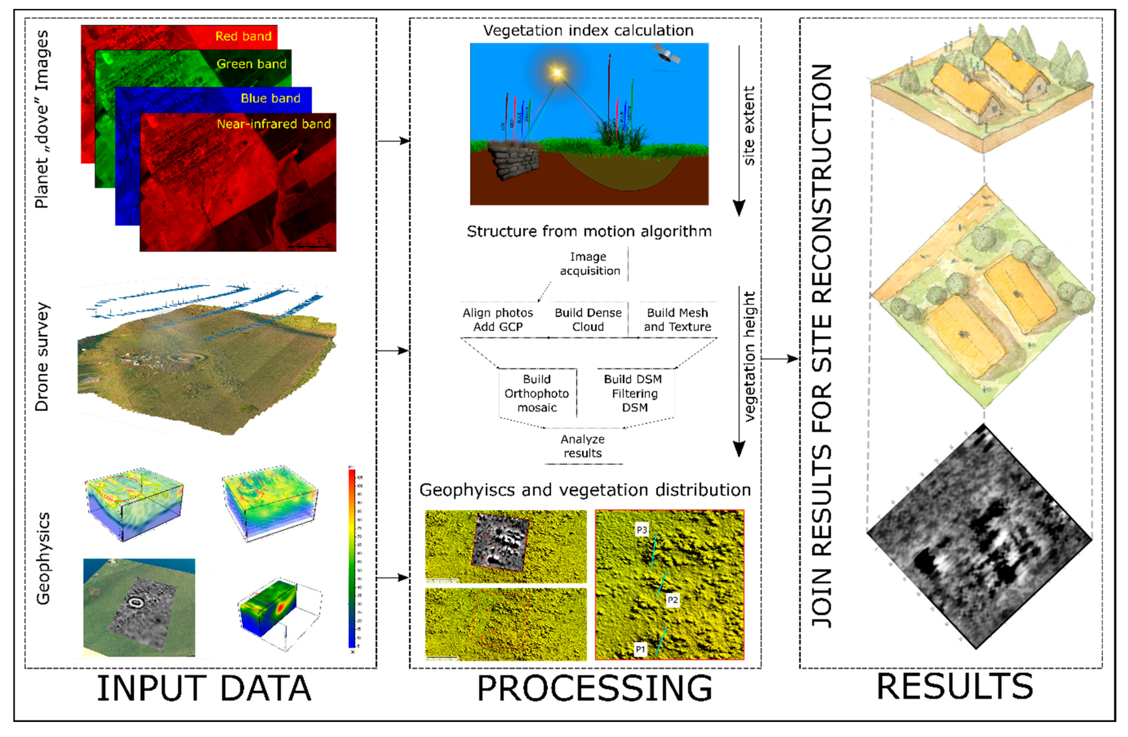
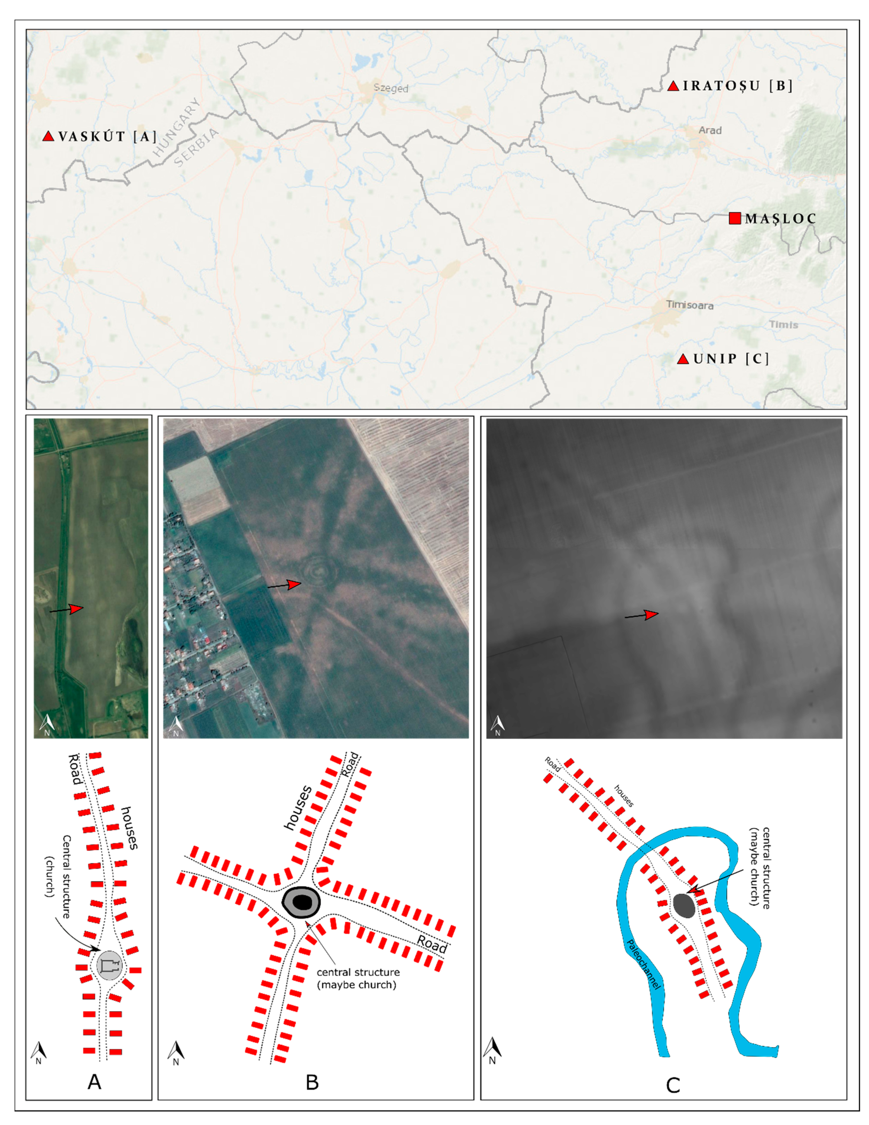
2. Study Area
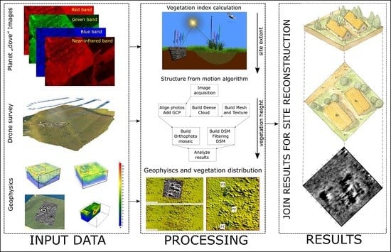
3. Materials and Methods
3.1. Geomorphometric Analyses
3.2. Planet Labs Satellite Images
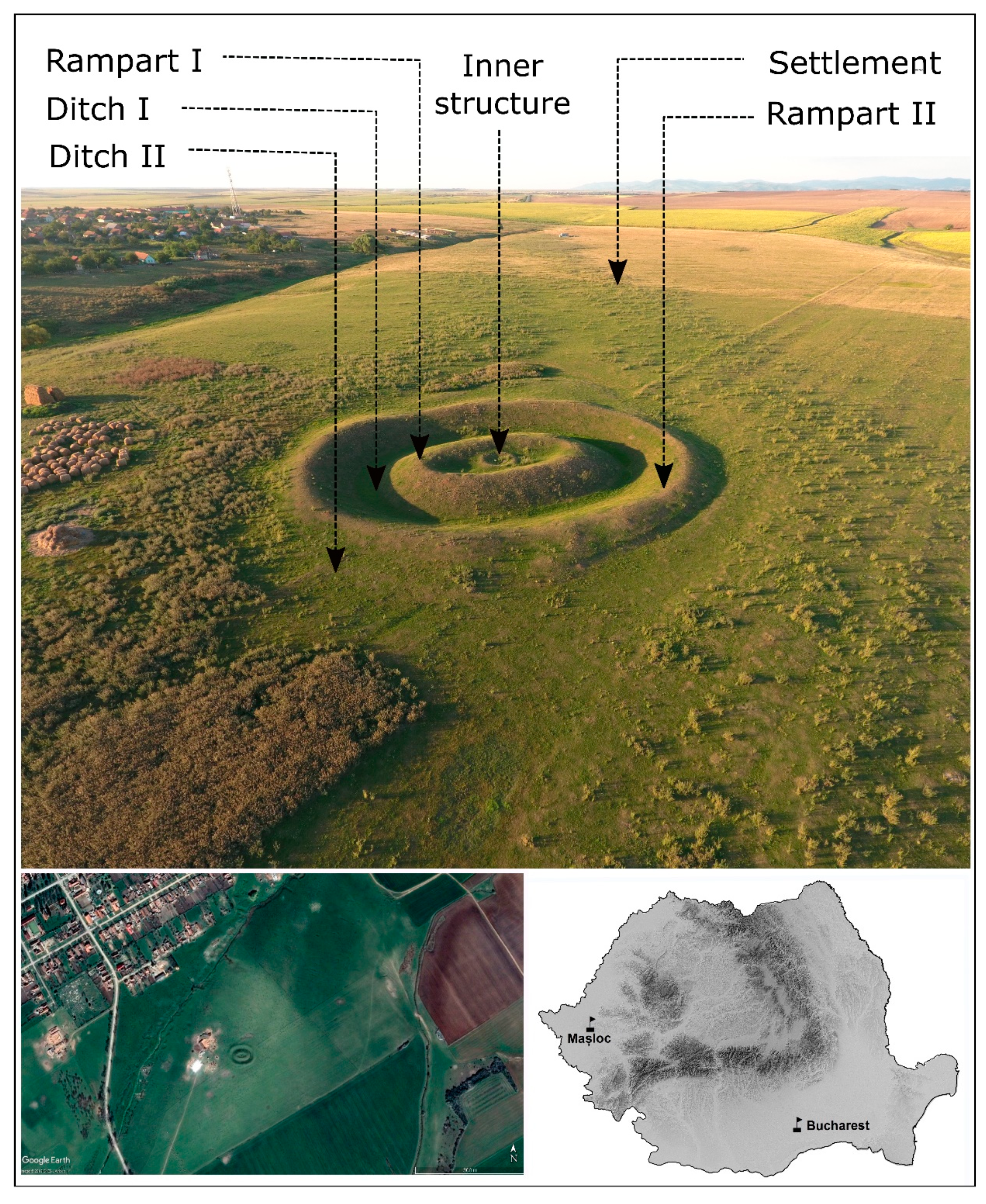
3.3. Physical Properties and Description of Vegetation Indices
3.4. UAV Survey
3.5. Geophysical Survey
4. Results
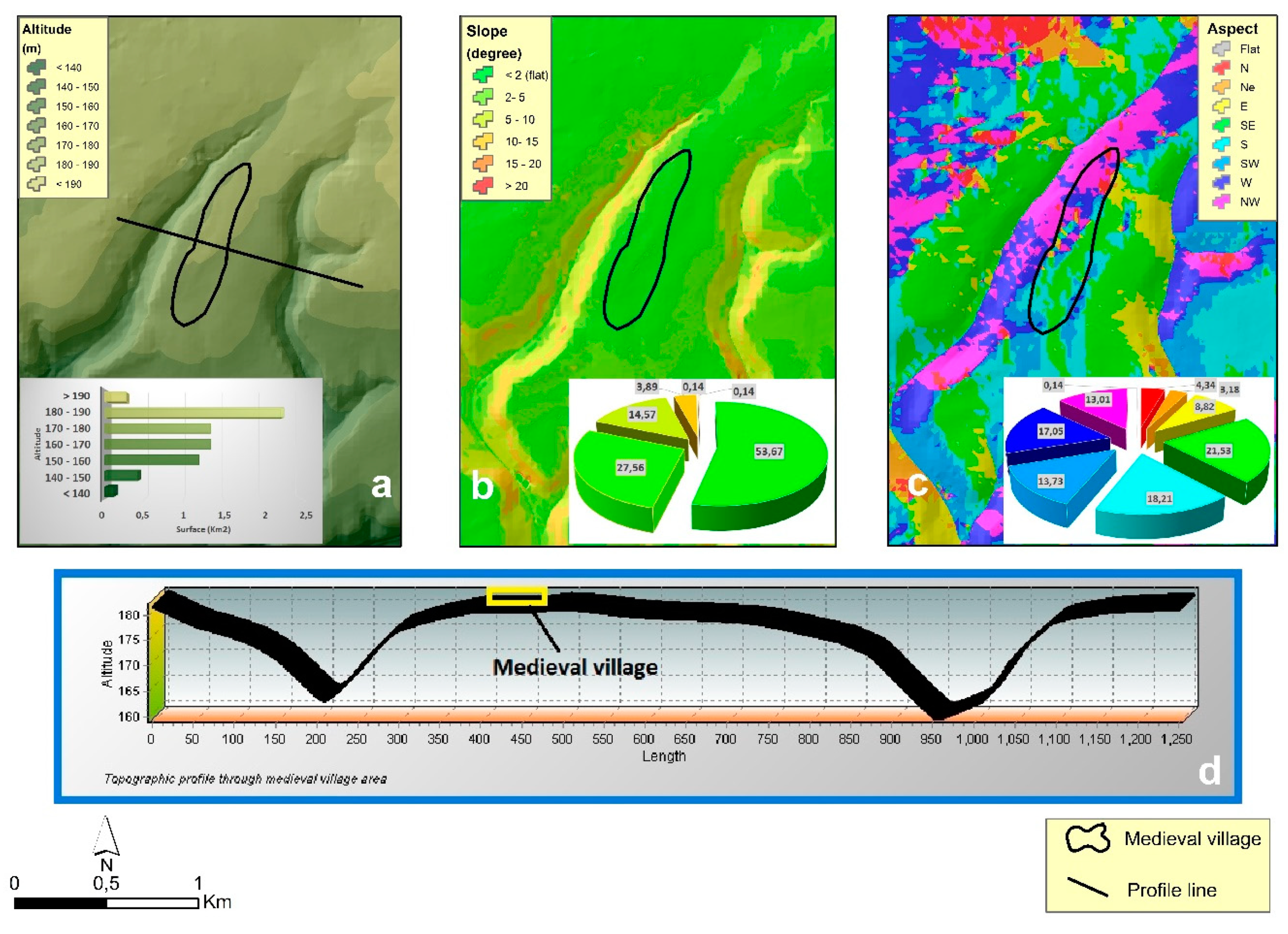
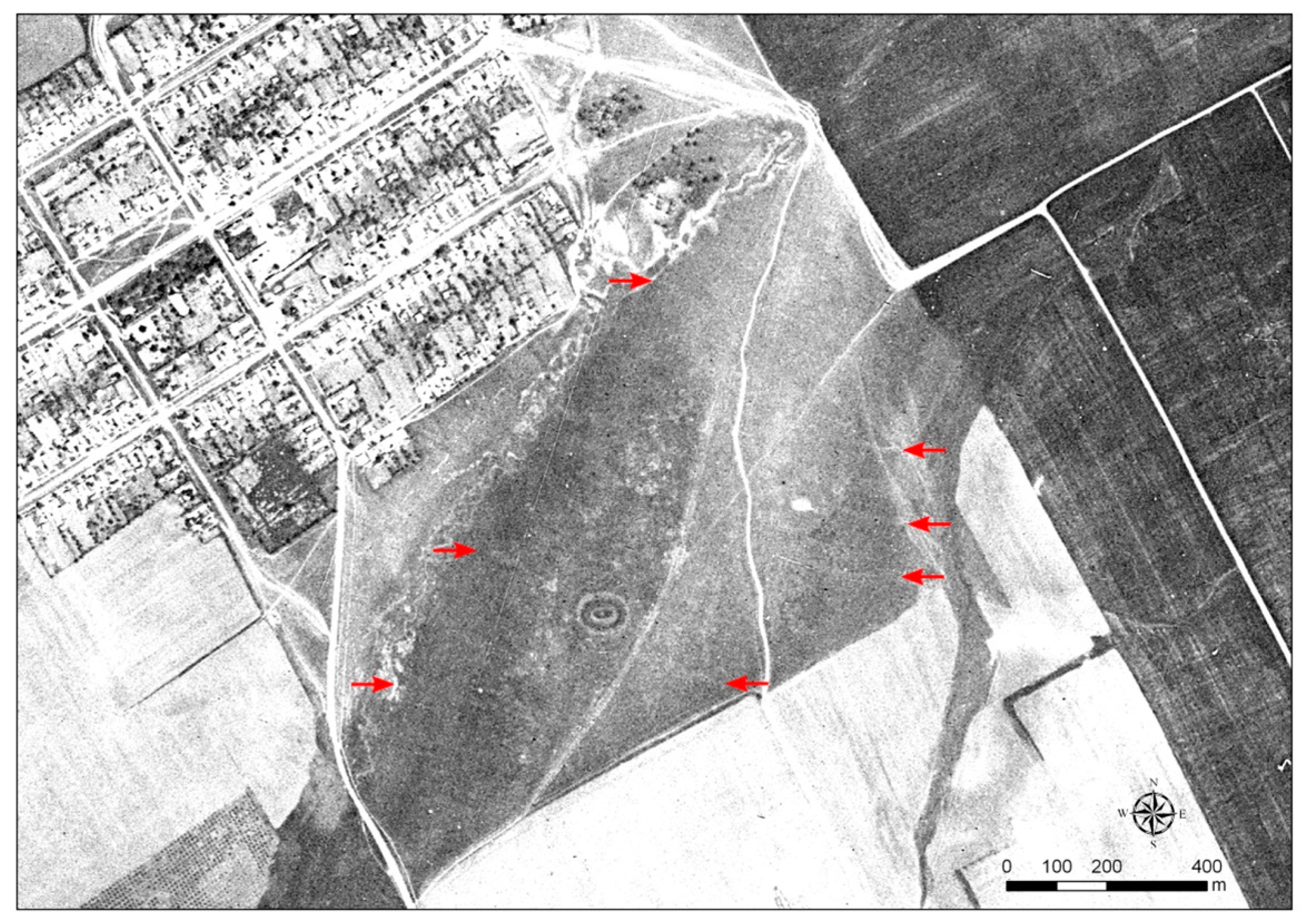
4.1. Geomorphometrically Characterization of the Medieval Village Location
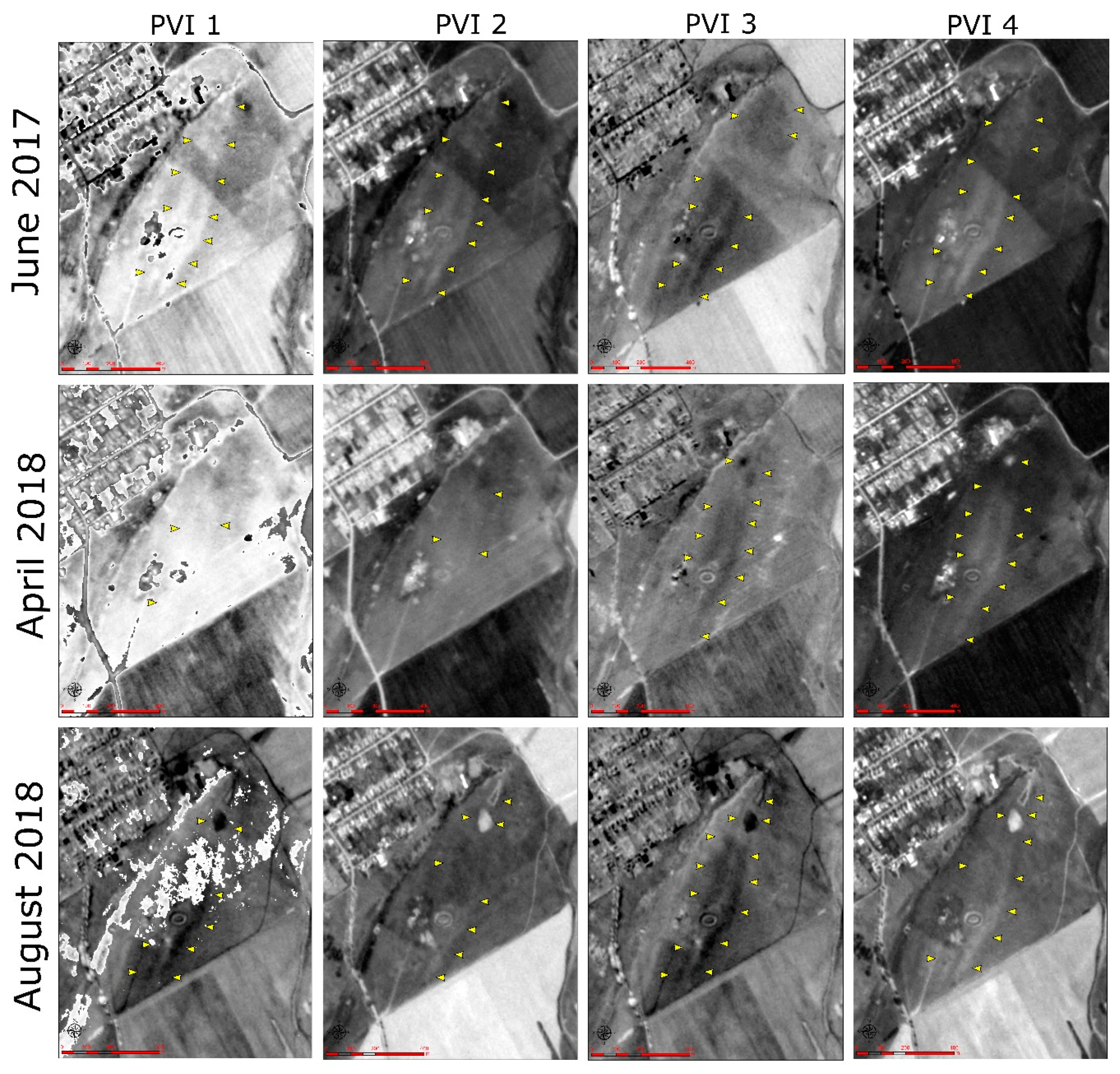
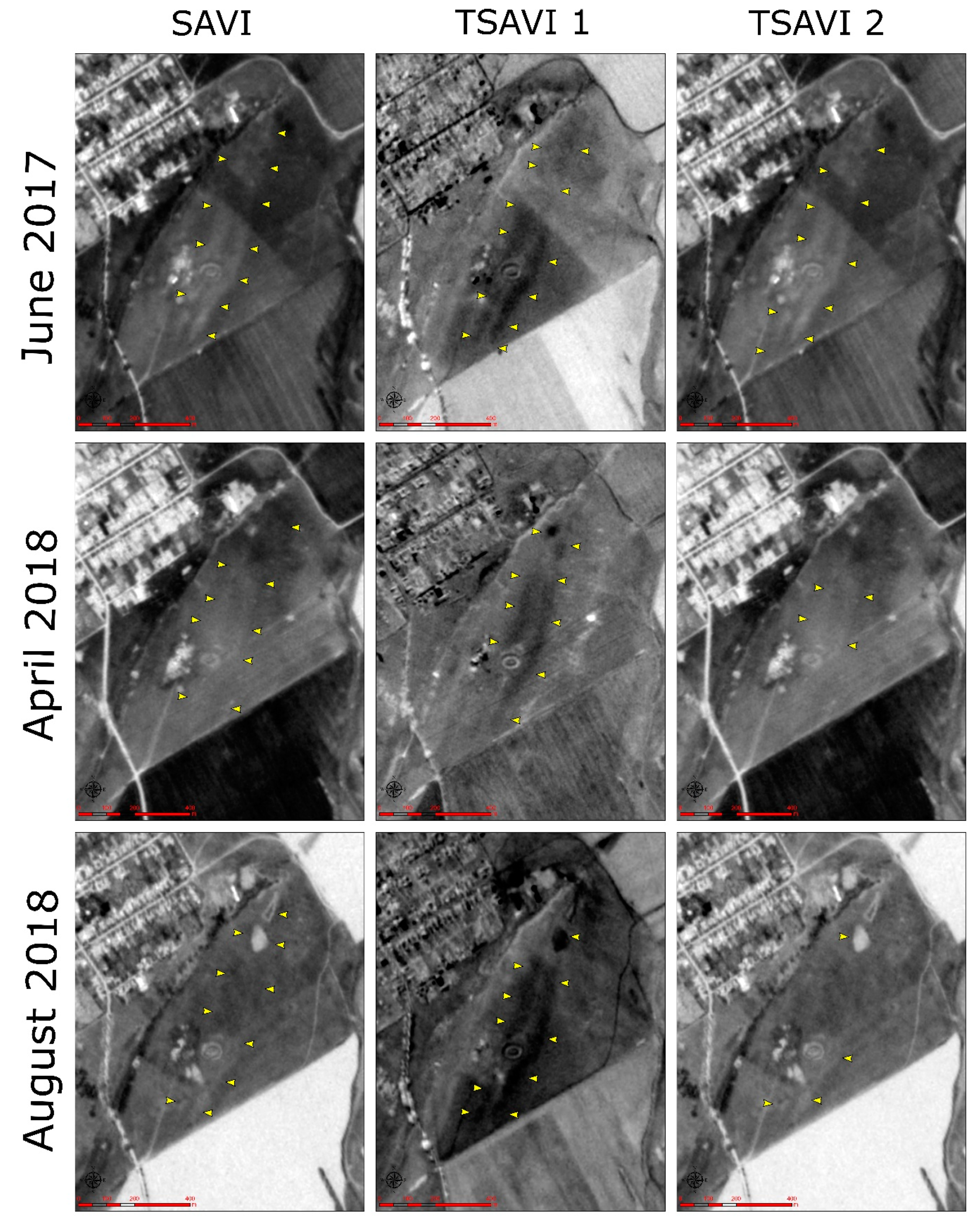
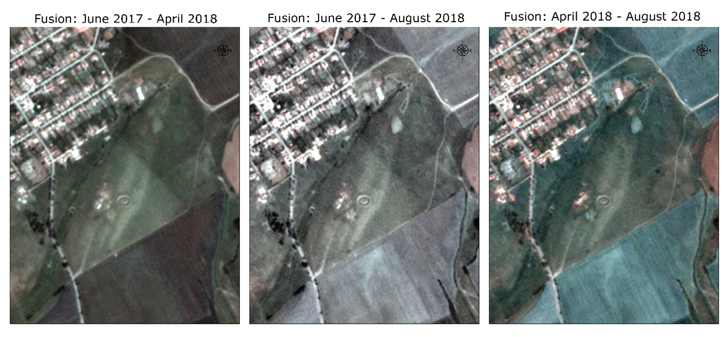
4.2. Integration of Vegetation Indices with Geophysics and Structure from Motion
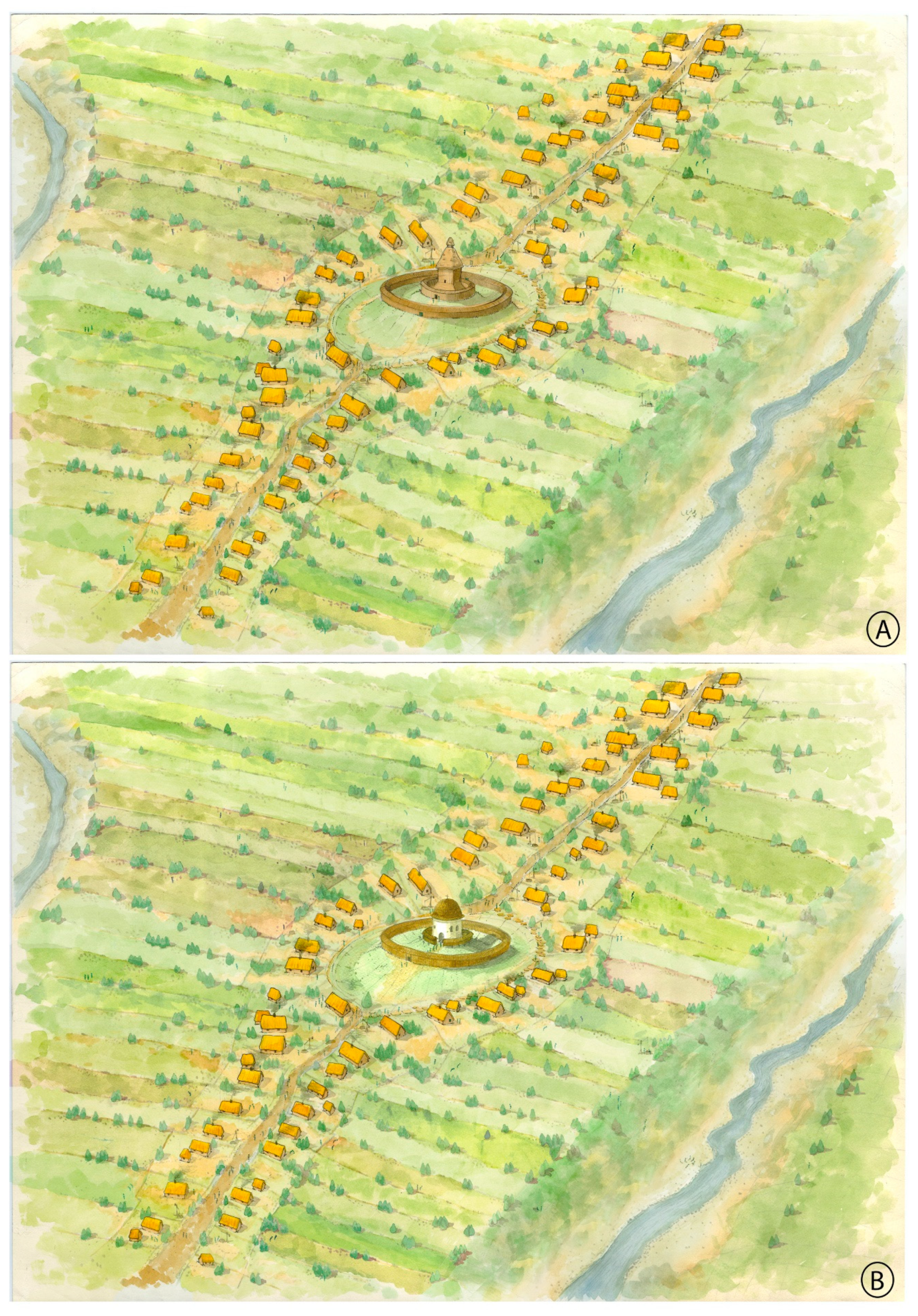
5. Discussions
6. Conclusions
Author Contributions
Funding
Acknowledgments
Conflicts of Interest
References
- Agapiou, A. Optimal Spatial Resolution for the Detection and Discrimination of Archaeological Proxies in Areas with Spectral Heterogeneity. Remote Sens. 2020, 12, 136. [Google Scholar] [CrossRef]
- Bennett, R.; Welham, K.; Hill, R.A.; Ford, A.L.J. The application of vegetation indices for the prospection of archaeological features in grass-dominated environments. Archaeol. Prospect. 2012, 19, 209–218. [Google Scholar] [CrossRef]
- Biagetti, S.; Merlo, S.; Adam, E.; Lobo, A.; Conesa, F.C.; Knight, J.; Bekrani, H.; Crema, E.R.; Alcaina-Mateos, J.; Madella, M. High and Medium Resolution Satellite Imagery to Evaluate Late Holocene Human–Environment Interactions in Arid Lands: A Case Study from the Central Sahara. Remote Sens. 2017, 9, 351. [Google Scholar] [CrossRef]
- Calleja, J.F.; Pagés, O.R.; Díaz-Álvarez, N.; Peón, J.; Gutiérrez, N.; Martín-Hernández, E.; Relea, A.C.; Melendi, D.R.; Álvarez, P.F. Detection of buried archaeological remains with the combined use of satellite multispectral data and UAV data. Int. J. Appl. Earth Obs. Geoinf. 2018, 73, 555–573. [Google Scholar] [CrossRef]
- Crawford, O.G.S. Archaeology in the Field; Phoenix House: London, UK, 1953. [Google Scholar]
- Fowler, M.L. Middle Mississippian agricultural fields. Am. Antiq. 1969, 34, 365–375. [Google Scholar] [CrossRef]
- Lasaponara, R.; Masini, N. Detection of archaeological crop marks by using satellite QuickBird multispectral imagery. J. Archaeol. Sci. 2007, 34, 214–221. [Google Scholar] [CrossRef]
- Parrington, M. Geophysical and Aerial Prospecting Techniques at Valley Forge National Historical Park, Pennsylvania. J. Field Archaeol. 1979, 6, 193–201. [Google Scholar]
- Melillos, G.; Themistocleous, K.; Papadavid, G.; Agapiou, A.; Prodromou, M.; Michaelides, S.; Hadjimitsis, D.G. Integrated use of field spectroscopy and satellite remote sensing for defence and security applications in Cyprus. In Proceedings of the Fourth International Conference on Remote Sensing and Geoinformation of the Environment (RSCy2016); International Society for Optics and Photonics: Bellingham, WA, USA, 2016; Volume 9688, p. 96880F. [Google Scholar]
- Poirier, N.; Hautefeuille, F.; Calastrenc, C. L’utilisation des micro-drones pour la prospection archéologique à basse altitude. Rev. Française Photogrammétrie Télédétection 2017, 213, 81–94. [Google Scholar]
- Holliday, V.T.; Gartner, W.G. Methods of soil P analysis in archaeology. J. Archaeol. Sci. 2007, 34, 301–333. [Google Scholar] [CrossRef]
- Malhotra, H.; Sharma, S.; Pandey, R. Phosphorus Nutrition: Plant Growth in Response to Deficiency and Excess. In Plant Nutrients and Abiotic Stress Tolerance; Springer: Berlin, Germany, 2018; pp. 171–190. [Google Scholar]
- Fernández-Hernandez, J.; González-Aguilera, D.; Rodríguez-Gonzálvez, P.; Mancera-Taboada, J. Image-based modelling from unmanned aerial vehicle (UAV) photogrammetry: An effective, low-cost tool for archaeological applications. Archaeometry 2015, 57, 128–145. [Google Scholar] [CrossRef]
- Davis, D.S.; Andriankaja, V.; Carnat, T.L.; Chrisostome, Z.M.; Colombe, C.; Fenomanana, F.; Hubertine, L.; Justome, R.; Lahiniriko, F.; Léonce, H. Satellite-based remote sensing rapidly reveals extensive record of Holocene coastal settlement on Madagascar. J. Archaeol. Sci. 2020, 115, 105097. [Google Scholar] [CrossRef]
- Kirk, S.D.; Thompson, A.E.; Lippitt, C.D. Predictive modeling for site detection using remotely sensed phenological data. Adv. Archaeol. Pr. 2016, 4, 87–101. [Google Scholar] [CrossRef]
- Crawford, O.G.S. A Century of Air-photography. Antiquity 1954, 28, 206–210. [Google Scholar] [CrossRef]
- Wilson, D.R. Air Photo Interpretation for Archaeologists; 2nd Revised; The History Press Ltd.: Stroud, UK, 2000; ISBN 0752414984. [Google Scholar]
- Kobyliński, Ł.M. Klasyfikacja Archeologicznych zdjęć Lotniczych na Podstawie Odkrytej Wiedzy. Ph.D. Thesis, Instytut Informatyki, Warsaw, Poland, February 2005. [Google Scholar]
- Pisz, M.; Timoc, C. All roads lead toTibiscum—Results and perspectives of the non-destructive landscape survey of the roman fort and its surroundings. ArheoVest 2015, Nr. III: I, 441–455. [Google Scholar]
- Eisenbeiss, H.; Sauerbier, M. Investigation of UAV systems and flight modes for photogrammetric applications. Photogramm. Rec. 2011, 26, 400–421. [Google Scholar] [CrossRef]
- Sauerbier, M.; Eisenbeiss, H. Uavs for the Documentation of Archaeological Excavations. In Proceedings of the International Archives of Photogrammetry, Remote Sensing and Spatial Information Sciences, Newcastle, UK, 21–24 June 2010. [Google Scholar]
- Verhoeven, G. Taking computer vision aloft—Archaeological three-dimensional reconstructions from aerial photographs with photoscan. Archaeol. Prospect. 2011, 18, 67–73. [Google Scholar] [CrossRef]
- Campana, S. Drones in Archaeology. State-of-the-art and Future Perspectives. Archaeol. Prospect. 2017, 24, 275–296. [Google Scholar] [CrossRef]
- Hegyi, A.; Urdea, P.; Floca, C.; Ardelean, A.; Onaca, A. Mapping the subsurface structures of a lost medieval village in South-Western Romania by combining conventional geophysical methods. Archaeol. Prospect. 2019, 26, 21–32. [Google Scholar] [CrossRef]
- Hegyi, A.; Vernica, M.; Drăguţ, L. An object-based approach to support the automatic delineation of magnetic anomalies. Archaeol. Prospect. 2020, 27, 3–12. [Google Scholar] [CrossRef]
- DL 71208 Magyar Nemzeti Levéltár Országos Levéltár (MNL OL) Budapest, HU, Collectio Diplomatica Hungarica/Diplomatikai Levéltár, Diplomatikai leveltár. Available online: https://archives.hungaricana.hu/en/charters/19941/ (accessed on 15 June 2020).
- Rationes Collectorum Pontificiorum in Hungaria / Pápai tized-szedők számadásai. 1281–1375; Monumenta Vaticana. Historiam Regni Hungariæ illustrantia / Vatikáni Magy. Okirattár, Ser. Prima. Tomus Primus./Első Sor. Első Kötet., Bp.; 1887; p. 146.
- Ionaşcu, I.; Lăzărescu-Ionescu, L.; Cîmpina, B.; Stănescu, E.; Prodan, D.; Roller, M. Documente Privind Istoria României. Veacul XIV C Transilvania, Volumul 3; Editura Didactică Şi Pedagogică: Bucuresti, Romania, 1954; Volume 224. [Google Scholar]
- Kristó, G. Anjou-kori Oklevéltár / Documenta res Hungaricas Tempore Regum Andegavensium Illustrantia: 1301–1387; Budapest-Szeged; Nemzeti Kulturális Örökség Minisztériuma: Budapest, Hungary, 2000; Volume VI: 1321–1322, ISBN 963 482 498 6. p. 325 (886). [Google Scholar]
- Mályusz, E. Zsigmondkori Oklevéltár: 1387-1399; Akadémiai Kiadó: Budapest, Hungary, 1951; Volume 1, p. 400 (3656). [Google Scholar]
- Pesty, F. Krassó vármegye története, Harmadik Kötet. (Oklevéltár. [1230–1518]); Krassó-Szörény Vármegye Közönsége; Az Athenaeum R[észvény]; Társ[ulat]: Budapest, Hungary, 1882; p. 429 (326). [Google Scholar]
- DL 93453 (Magyar Nemzeti Levéltár Országos Levéltár (MNL OL) Budapest, HU, Collectio Diplomatica Hungarica / Diplomatikai Levéltár. Available online: https://archives.hungaricana.hu/en/charters/198804/ (accessed on 15 June 2020).
- Pálffy, G. Egy rendkívüli forrás a magyar politikai elit 16. századi földrajzi ismereteiről. Az 1526 és 1556 között török kézbe került magyarországi városok, várak és kastélyok összeírása a Német-római Birodalom rendjei számára. In Várak Nyomában. Tanulmányok A 60 Éves Feld István Tiszteletére/Auf Den Spuren Der Burgen Jubil. Zum 60. Geburtstag Des Ung. Archaeol. Istvan Fried, Szerk; Terei György—Kovács Gyöngyi—Domokos György—Miklós Zsuzsa—Mordovin Maxim; Castrum Bene Egyesület, Civertan Grafikai Stúdió: Budapest, Hungary, 2011; ISBN 9789630824859, 963082485X. p. 193 (244). [Google Scholar]
- Szentkláray, J. Száz év Dél-Magyarország újabb történetéből: 1779-től napjainkig: Tekintettel a II. Károly és Mária Terézia korabeli előzményekre; Csanád-Egyház-megyei Könyvnyomda: Temesvár, Timiș, 1879; p. 24. [Google Scholar]
- Roos, M. Providentia Augustorum: Unter der Obhut der Kaiser: Dokumente zu den Anfängen des Temescher Banats: 1716-1739; Im Selbstverlag des Verfassers sowie im Verlag Musik Südo: Temeswar, Romania, 2018; ISBN 978-3-9390-4127-6. p. 81. [Google Scholar]
- Lipova’s district map (1718) (authorless). Mappa\Von dem\Lippovaer und Facseter\District\Worinnen alle bewohnte Dorfschafften, Sambt denen Prædien,\Flussen, Berg und Waldungen enthalten, nach vorgenommener\accurater Geometrischen abmessung Im Jahr 1718 & 1719. Manuscript map, color copy. Available online: http://maps.hungaricana.hu/hu/47915/ (accessed on 15 June 2020).
- Timișoara’s district map (1720) (authorless). Mappa\Von dem Temesva[r]er. District.\Worinen Alle Bewohnte Dorffschafften, Sambt denen Prædien, Flüssen, bäch, Morasten, und\Waldungen Enthalten, nach Vorgenommener Geometrischer accurater Abmessung\Im Jahr 1720. Manuscript map, color copy. Available online: http://maps.hungaricana.hu/hu/47936/ (accessed on 15 June 2020).
- Surdu, B. Aspecte privitoare la situaţia Banatului în 1743. In Anuarul Institutului de Istorie din Cluj; Editura Academiei Române: Bucureşti, Romania; Volume XIII, 1970; pp. 52/46–55/49. [Google Scholar]
- Mildenberger, P. Blumenthal im Banat; Heimatortsgemeinschaft Blumenthal; Bader Druck GmbH: Göppingen, Germany, 1990; 352 pg.; p. 68. [Google Scholar]
- Vertan, M. Sigilii de Sate, Comune şi târguri din Banatul Istoric (Secolele XVIII-XIX): Catalog; Editura Brumar: Timişoara, Romania, 2006; 92 pg.; ISBN 973-602-194-7, 978-973-602-194-7. p. 56, 86 (383. c). [Google Scholar]
- Evans, I.S. General geomorphometry, derivatives of altitude, and descriptive statistics. In Spatial Analysis in Geomorphology; 2019; ISBN 9781000000252. [Google Scholar] [CrossRef]
- Franklin, S.E. Geomorphometric processing of digital elevation models. Comput. Geosci. 1987. [Google Scholar] [CrossRef]
- Szypuła, B. Digital Elevation Models in Geomorphology. In Hydro-Geomorphology—Models and Trends; Shukla, D.P., Ed.; InTechOpen: London, UK, 2017; pp. 81–112. [Google Scholar] [CrossRef]
- De Boer, A.G.; Laan, W.N.H.; Waldus, W.; van Zijverden, W.K. LIDAR-based surface height measurements: Applications in archaeology. Beyond Illus. 2d 3d Digit. Technol. Tools Discov. Archaeol. Br. Arch. Rep. Int. Ser. 2008, 1805, 69–77. [Google Scholar]
- Verhagen, P.; Drăguţ, L. Object-based landform delineation and classification from DEMs for archaeological predictive mapping. J. Archaeol. Sci. 2012, 39, 698–703. [Google Scholar] [CrossRef]
- Team, P. Planet Application Program Interface: In Space for Life on Earth. San Fr. Ca 2017, 2017, 40. [Google Scholar]
- Ghuffar, S. DEM Generation from Multi Satellite PlanetScope Imagery. Remote Sens. 2018, 10, 1462. [Google Scholar] [CrossRef]
- Sozzi, M.; Marinello, F.; Pezzuolo, A.; Sartori, L. Benchmark of satellites image services for precision agricultural use. In Proceedings of the AgEng Conference, Wageningen, The Netherlands, 8–12 July 2018; pp. 8–11. [Google Scholar]
- Jensen, J.R. Remote Sensing of the Environment: An Earth resource Perspective 2/e; Pearson Education India: Chennai, India, 2009; ISBN 8131716805. [Google Scholar]
- Agapiou, A.; Hadjimitsis, D.G.; Alexakis, D.D. Evaluation of broadband and narrowband vegetation indices for the identification of archaeological crop marks. Remote Sens. 2012, 4, 3892–3919. [Google Scholar] [CrossRef]
- Mróz, M.; Sobieraj, A. Comparison of several vegetation indices calculated on the basis of a seasonal SPOT XS time series, and their suitability for land cover and agricultural crop identification. Tech. Sci. 2004, 7, 39–66. [Google Scholar]
- Silleos, N.G.; Alexandridis, T.K.; Gitas, I.Z.; Perakis, K. Vegetation indices: Advances made in biomass estimation and vegetation monitoring in the last 30 years. Geocarto Int. 2006, 21, 21–28. [Google Scholar] [CrossRef]
- Xue, J.; Su, B. Significant remote sensing vegetation indices: A review of developments and applications. J. Sens. 2017, 2017. [Google Scholar] [CrossRef]
- Agapiou, A.; Hadjimitsis, D.G. Vegetation indices and field spectroradiometric measurements for validation of buried architectural remains: Verification under area surveyed with geophysical campaigns. J. Appl. Remote Sens. 2011, 5, 53554. [Google Scholar] [CrossRef]
- Agapiou, A.; Lysandrou, V.; Lasaponara, R.; Masini, N.; Hadjimitsis, D.G. Study of the variations of archaeological marks at neolithic site of Lucera, Italy using high-resolution multispectral datasets. Remote Sens. 2016, 8, 723. [Google Scholar] [CrossRef]
- Agapiou, A.; Lysandrou, V.; Hadjimitsis, D.G. Optical Remote Sensing Potentials for Looting Detection. Geosciences 2017, 7, 98. [Google Scholar] [CrossRef]
- Dahiya, S.; Garg, P.K.; Jat, M.K. A comparative study of various pixel-based image fusion techniques as applied to an urban environment. Int. J. Image Data Fusion 2013, 4, 197–213. [Google Scholar] [CrossRef]
- Jordan, C.F. Derivation of leaf-area index from quality of light on the forest floor. Ecology 1969, 50, 663–666. [Google Scholar] [CrossRef]
- Rouse, J., Jr.; Haas, R.H.; Schell, J.A.; Deering, D.W. Monitoring Vegetation Systems in the Great Plains with ERTS; NASA: Washington, DC, USA, 1974. [Google Scholar]
- Deering, D.W. Measuring" forage production" of grazing units from Landsat MSS data. In Proceedings of the 10th International Symposium of Remote Sensing of the Envrionment, Ann Arbor, MI, USA, 6 October 1975; pp. 1169–1198. [Google Scholar]
- Richardson, A.J.; Wiegand, C.L. Distinguishing vegetation from soil background information. Photogramm. Eng. Remote Sens. 1977, 43, 1541–1552. [Google Scholar]
- Perry Jr, C.R.; Lautenschlager, L.F. Functional equivalence of spectral vegetation indices. Remote Sens. Environ. 1984, 14, 169–182. [Google Scholar] [CrossRef]
- Walther, D.; Shabaani, S. Large Scale Monitoring of Rangelands Vegetation Using NOAA/AVHRR LAC Data: Application to the Rainy Seasons 1989/90 in Northern Kenya. Range Manag. Handb. Kenya 1991, 3, 4. [Google Scholar]
- Qi, J.; Chehbouni, A.; Huete, A.R.; Kerr, Y.H.; Sorooshian, S. A modified soil adjusted vegetation index. Remote Sens. Env. 1994, 48, 119–126. [Google Scholar] [CrossRef]
- Huete, A.R. A soil-adjusted vegetation index (SAVI). Remote Sens. Environ. 1988, 25, 295–309. [Google Scholar] [CrossRef]
- Baret, F.; Guyot, G.; Major, D.J. TSAVI: A vegetation index which minimizes soil brightness effects on LAI and APAR estimation. In Proceedings of the 12th Canadian Symposium on Remote Sensing Geoscience and Remote Sensing Symposium; IEEE: Piscataway, NJ, USA, 1989; Volume 3, pp. 1355–1358. [Google Scholar]
- Baret, F.; Guyot, G. Potentials and limits of vegetation indices for LAI and APAR assessment. Remote Sens. Environ. 1991, 35, 161–173. [Google Scholar] [CrossRef]
- De Reu, J.; Plets, G.; Verhoeven, G.; De Smedt, P.; Bats, M.; Cherretté, B.; De Maeyer, W.; Deconynck, J.; Herremans, D.; Laloo, P. Towards a three-dimensional cost-effective registration of the archaeological heritage. J. Archaeol. Sci. 2013, 40, 1108–1121. [Google Scholar] [CrossRef]
- Măruia, L.; Cîntar, A.; Bolcu, L.; Ardelean, M.; Micle, D.; Stavilă, A.; Borlea, O. ArheoGis: Baza de date a patrimoniului arheologic cuprins în Lista Monumentelor Istorice a judeţului Timiş: Rezultatele cercetărilor de teren; BioFlux: Cluj-Napoca, Romania, 2011; ISBN 978-606-81991-23-2. [Google Scholar]
- Condurateanu, B.; Constantinescu, S.; Popescu, I. Digital Atlas of Romania v11.17; Bucharest 2019.
- Torma, I. Mittelalterliche Ackerfeld-Spuren im Wald von Tamási (Komitat Tolna). Acta Archaeol. Acad. Sci. Hung. 1981, 33, 245–256. [Google Scholar]
- Laszlovszky, J. Agriculture in Medieval Hungary. In The Economy of Medieval Hungary; Brill: Leiden, The Netherlands, 2018; pp. 79–112. [Google Scholar]
- Horváth, P. Pálóczi Horváth András: Túrkeve története a honfoglalástól a török idők végéig (The History of Túrkeve from the Hungarian Conquest up to the end of the Turkish Period). Túrkeve Földje És Népe 1992, 49–112. [Google Scholar]
- Navrátil, V. Povrchový průzkum zaniklé středověké osady Dašovice a její zaniklé plužiny. Hist. Geogr. 1983, 21, 217–233. [Google Scholar]
- Nekuda, V. Pfaffenschlag-Zaniklá středověká ves u Slavonic; Blok: Brno, Czech Republic, 1975; p. 277. [Google Scholar]
- Buzás, K.; Frigyes, G.; Pánya, I. Középkori templomok nyomában Bács-Kiskun megyében II. VárakKastélyok Templ. 2019, 4, 16–19. [Google Scholar]
- Pánya, I. Possibilities and methods for the reconstruction of the settlement structure of medieval Bodrog county. Banatica 2020, 29, 321–358. [Google Scholar]
- Pădurean, E.D.; Dorogostaisky, L. Mistere cu privire la imaginea satelitară Google Earth a unui sit arheologic de la Iratoşu, jud. Arad Misteries regarding the Google Earth sattelite image of a archaeological sit from Iratosu, Arad County. An. Aradului 2016, 2, 11–22. [Google Scholar]
- Mărginean, F. Contributions to the Medieval Ecclesiastic Geography of Arad County. State of Research. Ziridava. Stud. Archaeol. 2018, 32, 195–220. [Google Scholar]
- Engel, P. The Realm of St Stephen, 1st ed.; International Library of Historical Studies, 19, I.B.; Tauris Publishers: London, UK, 2001; ISBN 1860640613. [Google Scholar]


| Name | Acquisition | Sensor | Orbit Direction | Resolution | |
|---|---|---|---|---|---|
| IMG 1 | 20170602_084526_0e26_3B_AnalyticMS | 2017-06-02T08:45:26+00:00 | Optical | Descending | 3 m |
| IMG 2 | 20180822_083312_0f4d_3B_AnalyticMS | 2018-08-22T08:33:12+00:00 | Optical | Descending | 3 m |
| IMG 3 | 20180411_101735_0c54_3B_AnalyticMS | 2018-04-11T10:17:35+00:00 | Optical | Descending | 3 m |
| Slope-based vegetation indices | ||
| Ratio Vegetation Index (RVI) | [58] | |
| Normalized Difference Vegetation Index (NDVI) | [59] | |
| Transformed Vegetation Index (TVI) | [60] | |
| Distance-based vegetation indices | ||
| Perpendicular Vegetation Index (PVI) | [61] | |
| Perpendicular Vegetation Index 1 (PVI1) | [62] | |
| Perpendicular Vegetation Index 2 (PVI2) | [63] | |
| Perpendicular Vegetation Index 3 (PVI3) | [64] | |
| Difference Vegetation Index (DVI) | [61] | |
| Soil Adjusted Vegetation Index (SAVI) | [65] | |
| Transformed Soil Adjusted Vegetation 1 (TSAVI1) | [66] | |
| Transformed Soil Adjusted Vegetation 2 (TSAVI2) | [67] | |
© 2020 by the authors. Licensee MDPI, Basel, Switzerland. This article is an open access article distributed under the terms and conditions of the Creative Commons Attribution (CC BY) license (http://creativecommons.org/licenses/by/4.0/).
Share and Cite
Hegyi, A.; Sarris, A.; Curta, F.; Floca, C.; Forțiu, S.; Urdea, P.; Onaca, A.; Timofte, F.; Pisz, M.; Timuț, S.; et al. Deserted Medieval Village Reconstruction Using Applied Geosciences. Remote Sens. 2020, 12, 1975. https://doi.org/10.3390/rs12121975
Hegyi A, Sarris A, Curta F, Floca C, Forțiu S, Urdea P, Onaca A, Timofte F, Pisz M, Timuț S, et al. Deserted Medieval Village Reconstruction Using Applied Geosciences. Remote Sensing. 2020; 12(12):1975. https://doi.org/10.3390/rs12121975
Chicago/Turabian StyleHegyi, Alexandru, Apostolos Sarris, Florin Curta, Cristian Floca, Sorin Forțiu, Petru Urdea, Alexandru Onaca, Fabian Timofte, Michał Pisz, Sergiu Timuț, and et al. 2020. "Deserted Medieval Village Reconstruction Using Applied Geosciences" Remote Sensing 12, no. 12: 1975. https://doi.org/10.3390/rs12121975
APA StyleHegyi, A., Sarris, A., Curta, F., Floca, C., Forțiu, S., Urdea, P., Onaca, A., Timofte, F., Pisz, M., Timuț, S., Nica, M., Maciulschi, D., & Stavilă, A. (2020). Deserted Medieval Village Reconstruction Using Applied Geosciences. Remote Sensing, 12(12), 1975. https://doi.org/10.3390/rs12121975