Optimal Walker Constellation Design of LEO-Based Global Navigation and Augmentation System

Abstract

Low Earth orbit (LEO) satellites located at altitudes of 500 km~1500 km can carry much stronger signals and move faster than medium Earth orbit (MEO) satellites at about a 20,000 km altitude. Taking advantage of these features, LEO satellites promise to make contributions to navigation and positioning where global navigation satellite system (GNSS) signals are blocked as well as the rapid convergence of precise point positioning (PPP). In this paper, LEO-based optimal global navigation and augmentation constellations are designed by a non-dominated sorting genetic algorithm III (NSGA-III) and genetic algorithm (GA), respectively. Additionally, a LEO augmentation constellation with GNSS satellites included is designed using the NSGA-III. For global navigation constellations, the results demonstrate that the optimal constellations with a near-polar Walker configuration need 264, 240, 210, 210, 200, 190 and 180 satellites with altitudes of 900, 1000, 1100, 1200, 1300, 1400 and 1500 km, respectively. For global augmentation constellations at an altitude of 900 km, for instance, 72, 91, and 108 satellites are required in order to achieve a global average of four, five and six visible satellites for an elevation angle above 7 degrees with one Walker constellation. To achieve a more even coverage, a hybrid constellation with two Walker constellations is also presented. On this basis, the GDOPs (geometric dilution of precision) of the GNSS with and without an LEO constellation are compared. In addition, we prove that the computation efficiency of the constellation design can be considerably improved by using master–slave parallel computing.

1. Introduction

With the completion of the construction of China’s BeiDou navigation satellite system (BDS) in 2020, all global navigation satellite systems will be capable of offering global service [1]. Along with two regional navigation satellite systems—the quasi-zenith satellite system (QZSS) from Japan and navigation with Indian constellation (NavIC) from India—medium/geosynchronous/inclined geosynchronous orbit satellites, whose altitudes are approximately 20,000 km, constitute the satellite navigation system. However, due to the weak signals of these satellites, the positioning, navigation and timing (PNT) services, on which many critical infrastructures are heavily dependent, are easily disrupted in a deeply attenuated environment or can be interfered with by a jammer [2]. To avoid this limitation, the low Earth orbit (LEO)-augmented global navigation satellite system (GNSS) has attracted increased attention. Experimental results from a satellite time and location (STL) service carried out by Iridium show that, even on the lowest floor inside a building, the carrier-to-noise density power ratio (C/N0) from Iridium satellites ranges between 35 and 55 dB-Hz, which is approximately the same as GPS in an open sky environment [3]. Stronger signals would make GNSS more resilient and resistant to jamming. In addition, simulation results show that the swifter motion of LEO satellites significantly reduces by 70%~90% the convergence time of the precise point positioning (PPP), and the tracking data of GNSS satellites from LEO satellites improves the accuracy of the precise orbit determination of GNSS by 70% [4,5,6]. Thus, the LEO-augmented GNSS promises to make a considerable contribution to PNT services.

The prerequisite of the LEO-augmented GNSS service is a well-distributed LEO satellite constellation augmentation or a standalone backup navigation system. LEO satellite constellations consist of small satellites. Small satellites have greater component capabilities and low developing, building and launching costs. Small satellites have led to the wider application of large constellations in space missions, such as in telecommunication, the survey of resources and climate and sustaining global information networks, as well as navigation [7,8,9,10]. The construction of LEO constellations consisting of small satellites can be completed within a short time. However, because of the LEO’s much smaller footprint than the medium Earth orbit (MEO) satellite, many more satellites would be needed in order to provide the same coverage as an MEO [11]. The emerging mega-constellations proposed by SpaceX, Telesat and OneWeb for internet broadband are great opportunities for integrating communication and navigation, but their huge costs and redundancy make these constellations less attractive [12]. With the first successful launch of a trial satellite, China’s LEO-based augmentation system—Hongyan—is under construction [13]. Therefore, the entire design routine of a well-distributed LEO global coverage constellation is important and in urgent demand.

Among all the existing navigation constellations, the Walker configuration is widely used in the global positioning system (GPS), Galileo, and global navigation satellite system (GLONASS), as well as the third-generation system of BDS (BDS-3) because of its symmetrical configuration and favourable global coverage. Walker configuration is denoted as N/P/F, where N represents the total number of satellites in a constellation, P is the number of orbital planes and F is an inter-plane phase parameter, signifying the relative location of the satellites in the adjacent plane [14]. Besides this, many other configurations have also been figured out since the last century. Luders et al. introduced the streets-of-coverage design, in which the inclined circular orbit satellites were placed at the same altitude in a single plane, and several different planes were selected to achieve local or global coverage [15]. Mortari et al. introduced a flower-constellation methodology which was generally characterized by repeatable ground tracks [16]. The orbits in a flower constellation can be elliptical or circular, and the constellation can have zonal or global coverage, depending on the specific mission requirements. The satellites in the constellation share the same repeating ground track, perigee altitude, inclination and argument of perigee. Traditionally, analytical methods were mainly adopted in early constellation designs due to only a few satellites and the need for simple earth coverage. However, now, with hundreds or even thousands of satellites and the requirements of different tasks in a constellation, there is always a set of optimal solutions rather than one best solution. Therefore, constellation design has become a non-linear and multi-objective optimization problem.

Multi-objective optimization problems mean there is always a trade-off between objectives like the number of satellites and earth coverage. One of the tools which has proved to be effective in solving this problem is the genetic algorithm (GA). By combining several weighted objective functions into a single function, Ely et al. applied the GA for zonal elliptical streets of coverage in constellation design [17]. However, the results of the GA were highly related to weight, which was always difficult to choose. Thus, instead of a single objective optimization, Ferringer et al. implemented a multi-objective evolutionary algorithm—the non-dominated sorting genetic algorithm-II (NSGA-II)—to generate sets of constellations. The results demonstrated that this was effective in searching for the complex trade-off spaces in satellite constellation design. Compared to an enumerative analysis, the NSGA-II enabled great cost saving in computational resources. Furthermore, the results of multi-objective evolutionary algorithm paradigms based on the two parallel processes of master–slave and island models showed excellent approximations of the true Pareto frontier [18,19].

Aiming at LEO satellites, Lang developed a LEO satellite constellation specifically for continuous coverage of the mid-latitude band [20]. A regional augmentation system aiming at Chinese cities was designed by Zhang et al. in which the flower and Walker configurations with a restricted phasing scheme, as well as deployment strategies, were compared [21]. Furthermore, Shtark et al. proposed an optimization algorithm for regional positioning using a LEO satellite constellation [22]. The differences and similarities in the system architecture among three large broadband constellations—SpaceX, OneWeb and Telesat—were compared, and the total system throughput and minimum ground stations to support the system throughput were calculated by Portillo ID et al. [12]. Aiming at LEO-based even global coverage augmentation systems, Ma et al. designed an optimal hybrid configuration of 100 LEO satellites. Besides this, the necessary number of satellites for different visible satellites and the elevation mask angle were studied using the GA [23]. In the future, a LEO satellite constellation could either be an augmentation system in the environment, where the GNSS PNT service degrades, or a stand-alone backup navigation system, where the GNSS PNT service is not available. Therefore, it is essential to design LEO satellite constellations to fulfil both aspects.

The Walker constellation is preferred for navigation because of its symmetrical configuration. For a LEO-based global navigation constellation, a polar or near-polar inclination is required. A polar constellation might increase the chance of collision in the polar region, especially in a large constellation. Consequently, a near-polar Walker constellation is adopted in this paper. With the near-polar Walker constellation, a global navigation constellation solely consisting of LEO satellites is designed under two situations: one is the two-objective optimization case, including the geometric dilution of precision (GDOP), measuring the constellation geometry and number of satellites, and the other is the three-objective optimization case including the number of satellites, the GDOP and satellite altitude. The NSGA-III, a reference-based NSGA-II, is used for the two- and three-objective navigation constellation design. For any LEO-augmented constellation with a specific altitude, the single objective is the global average of visible satellites; therefore, the GA is adopted for the augmented constellation design. Since it is hard to achieve an even global coverage with a single near-polar Walker constellation, a hybrid constellation with Walker/Walker constellation is designed for an even global coverage. Furthermore, the Walker/Walker LEO constellation is designed with the consideration of GNSS satellites, and the GDOPs of GNSS with and without LEO constellation are compared. Since the constellation design process is time-consuming, a parallel processing method is adopted in order to improve computing efficiency.

This paper mainly gives solutions to LEO navigation constellation design every 100 km for altitudes of 900 km~1500 km. Besides this, LEO augmentation constellations are designed every 100 km for altitudes of 900 km~1500 km from the global average visible satellites perspective. In addition, the GDOPs of the GNSS with and without LEO constellation are compared. From the search results, we prove that NSGA-III is able to give optimal fronts of constellation design. The paper is organized as follows: Section 2 describes the problem and the methodology, the results and analysis are presented in Section 3; and the conclusions and discussion are presented in the last section.

2. Problem Description and Methodology

2.1. Problem Description

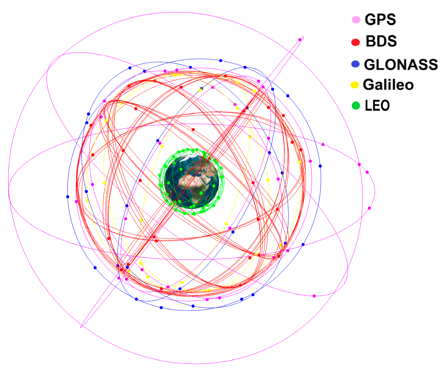
A Walker configuration has been widely used in navigation systems due to its symmetrical distribution and favourable global coverage. Owing to a remarkable difference in the footprints of a LEO and MEO, as shown in Figure 1, many more satellites would be required in order to provide global coverage. The nadir-pointing coverage circle area $A$ of a satellite is calculated as $\mathrm{A}=2\mathsf{\pi }{R}^{2}h/\left(R+h\right)$; $\mathrm{R}$ (6378.14 km) is the radius of Earth and $\mathrm{h}$ is the satellite altitude. For instance, taking the MEO altitude as 20,200 km and the LEO altitude as 900 km, the ratio of the footprint areas of MEO/LEO is 6.146.

In the problem description section, the Walker configuration and the factor-GDOP of measuring the positioning performance for a satellite constellation are described.

2.1.1. Walker Pattern

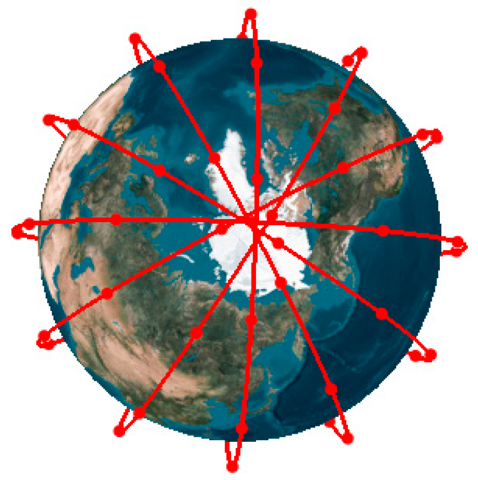
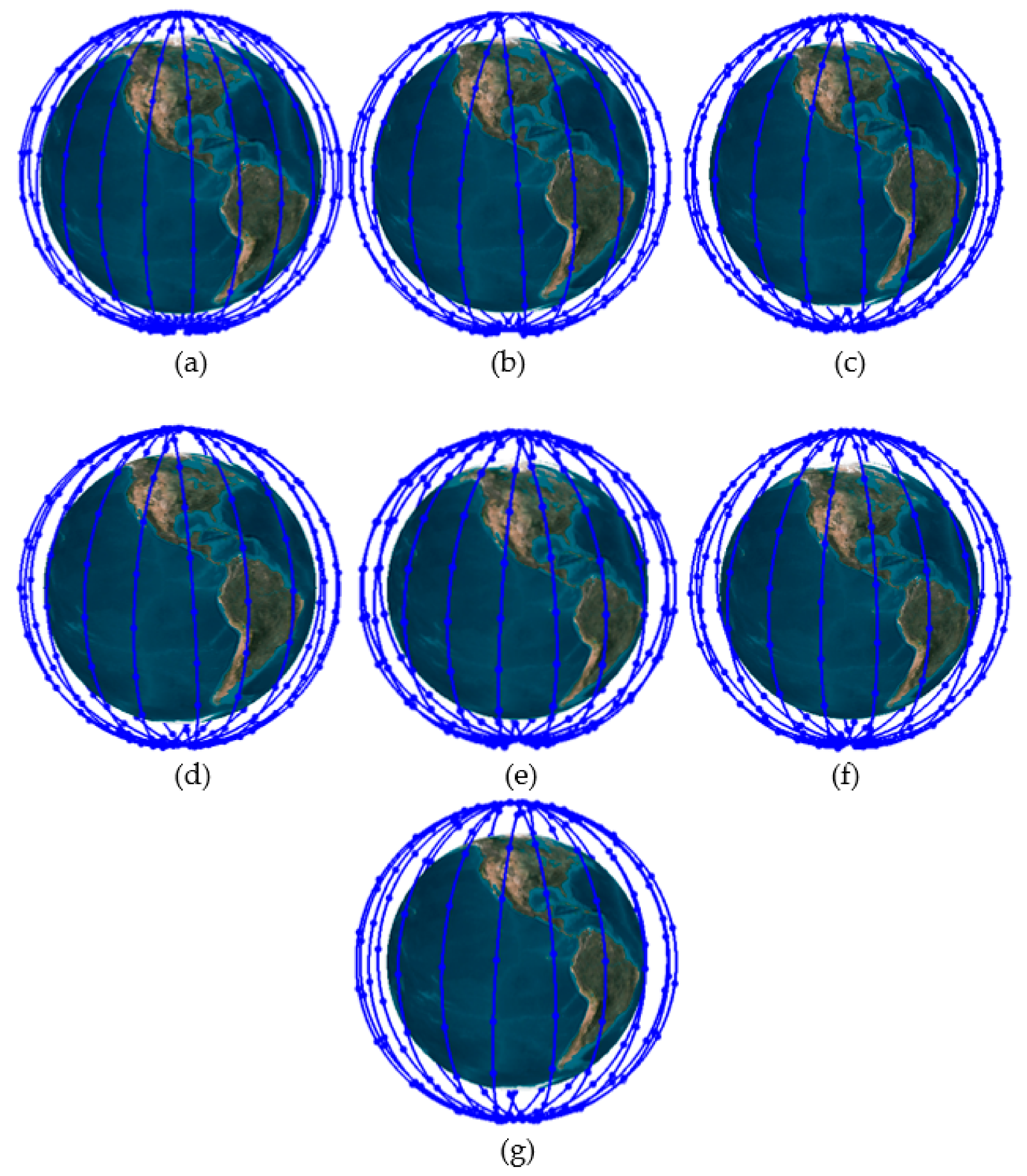
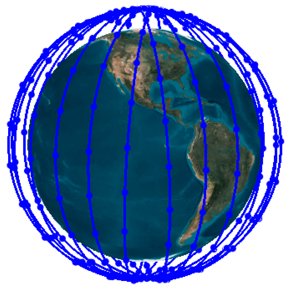
A Walker pattern constellation is described by three integers as N/P/F, where N denotes the total number of satellites in the constellation, P is the number of orbital planes and F is the phasing parameter, which defines the relative position of the satellites in the adjacent plane and values between 0 and P-1. Satellites in a Walker constellation are uniformly distributed in space. For instance, the distribution of satellites in the Iridium system, which is a Walker constellation, is depicted in Figure 2. These satellites share the same semi-major axis, inclination, eccentricity and argument of perigee. The right ascension of the ascending nodes (RAAN) and the mean anomaly of the j-th satellites on the i-th plane are described by the following formulas [24]:

$${\Omega }_{ij}=\frac{2\pi }{P}\left(i-1\right)$$

(1)

$$M_{ij}=\frac{2\pi }{S}\left(j-1\right)+\frac{2\pi }{N}F\left(i-1\right)$$

(2)

where $\mathrm{S}=\mathrm{N}/\mathrm{P}$ represents the number of satellites per plane, $\Omega$ is the $\mathrm{RAAN}$ and $\mathrm{M}$ is the mean anomaly. As such, satellites in a Walker configuration are specifically located.

2.1.2. GDOP

The problem of determining the user position, which concerns three unknown variables (i.e., Cartesian coordinates x, y, z), is solved through the known positions of navigation satellites. Usually, there is a time offset for the receiver clock; so, there are four unknown variables instead of three, meaning that there should be at least four satellites in sight at any time for determining the position of the user. The user position error is described as [25]:

$$\sigma =GDOP\cdot {\sigma }_{UERE}$$

(3)

where the GDOP solely depends on the relative locations of the satellites and the user. ${\sigma }_{UERE}$ is the pseudo-range error factor, mainly including the effects of the satellite clock, ionosphere error, troposphere error, receiver noise and multi-path. GDOP ranges from zero to infinity (∞), and the geometry is ideal when GDOP tends towards 0. The larger the GDOP value is, the poorer the geometry of the satellite constellation.

2.2. Methods

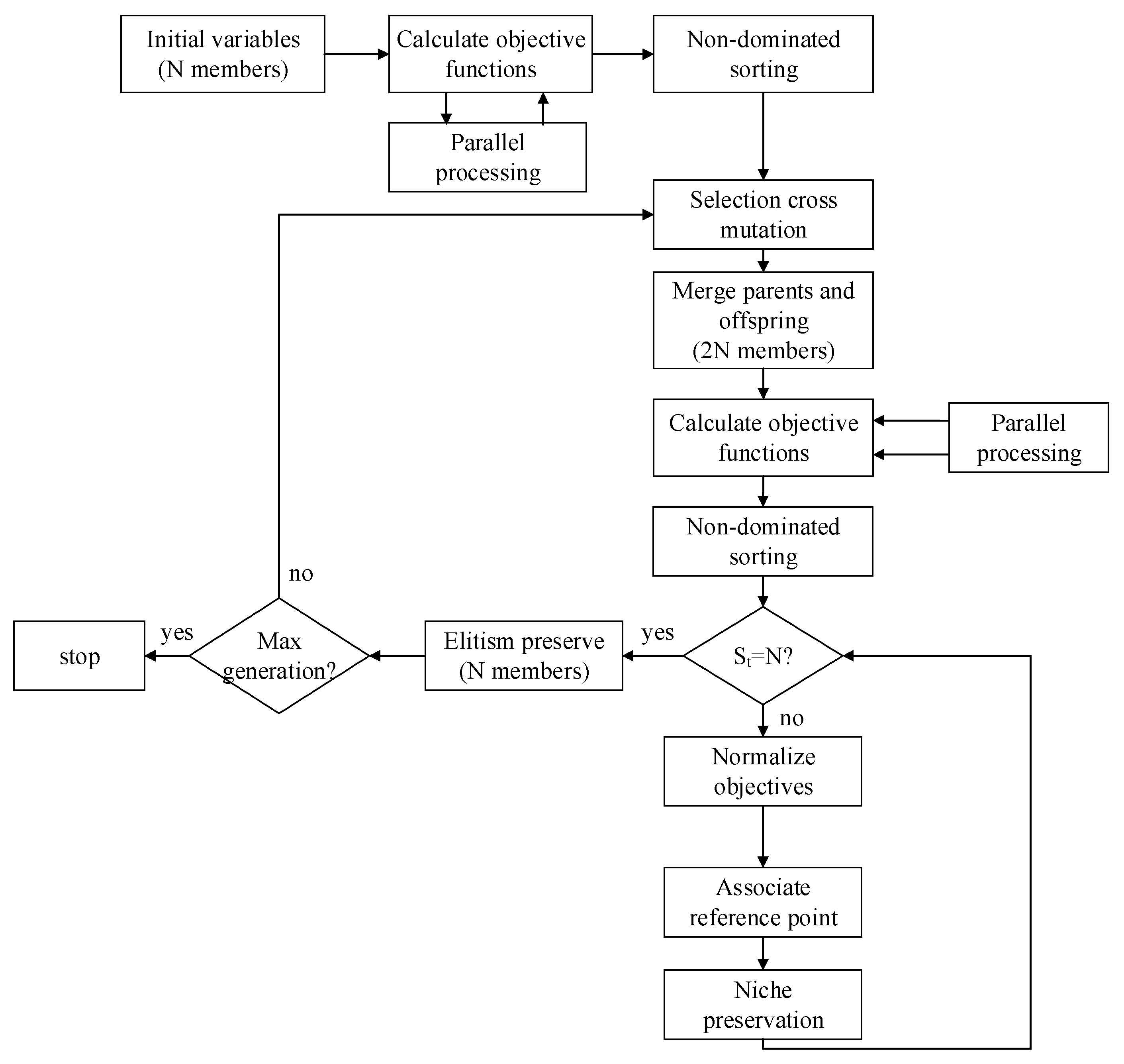
In order to get the optimal parameters to describe a Walker constellation, NSGA-III, one of the GAs, is used in this paper. GA mimics Darwin’s theory of evolution, creating offspring through a procedure of cross, mutation and fitness selection. The procedure begins by producing a random population, and each individual, coded by a chromosome, represents a possible solution to the problem. The chromosome could be binary-coded or real-coded. For a binary-coded chromosome, cross techniques may be a one-point or two-point crossover. With a cross probability, two parent chromosomes exchange the bits after the point with one-point crossover and the bits between the points with two-point crossover to create two new offspring. With the new offspring, a mutation technique changes a random gene of the chromosome to create a new offspring with a mutation probability. For a binary-coded chromosome, the gene changes from 0 to 1 or from 1 to 0. A mutation technique introduces new members to the population and prevents prematurity. Better individuals are preserved to the next generation in accordance with their fitness functions. For a minimum problem, individuals with smaller fitness functions are carried on to the next generation. This loop of cross, mutation and fitness functions stops when the maximum generation or a stop criterion is met. For a multi-objective problem, the results achieve a Pareto frontier, which means no solution in this set can be better than the current one in some objective function without worsening the other objective function.

NSGA-III is a reference-point based NSGA-II [26,27]. In NSGA-II, crowding distance sorting is adopted to ensure population diversity. We will give an overview of crowding distance sorting in advance in order to get a better understanding of reference point distance sorting. The routine of crowding distance sorting is as follows: firstly, objective functions are sorted for individuals in every non-domination layer. The maximum and minimum for the m-th objective function are denoted as $f_m^{\max }$ and $f_m^{\min }$, respectively. Next, crowding distance $i_d$ is calculated as $(f_m^{i+1}-f_m^{i-1})/(f_m^{\max }-f_m^{\min })$. An individual with a larger crowding distance is sent to the next generation. With a fast non-dominating and crowding distance sorting, the NSGA-II is able to reduce the computational complexity of the NSGA and preserve elitism. However, with an increase in objectives, on the one hand, the identification of neighbors could be rather difficult, which means crowding distance sorting lacks diversity preservation; on the other hand, the searching process could be rather time-consuming. With a strategy change in reference point distance sorting, the NSGA-III is able to alleviate the problems of sticking to multiple local fronts, the computationally expensive identification of neighbours and the difficulty in creating new solutions when it concerns an increase in the number of objectives. More comparisons of the NSGA-II and NSGA-III are listed in the reference section [28]. For NSGA-III, the algorithm starts with a random population $P_0$ of size $N$, and after being sorted by non-domination, each member in this population is assigned a rank. Then, the main loop starts with an offspring $P_t$ created from $P_0$ by the usual cross and mutation operators. After this, $P_t$ combines with its offspring $Q_t$ to form a population $R_t=P_t\cup Q_t$ of size $2N$. 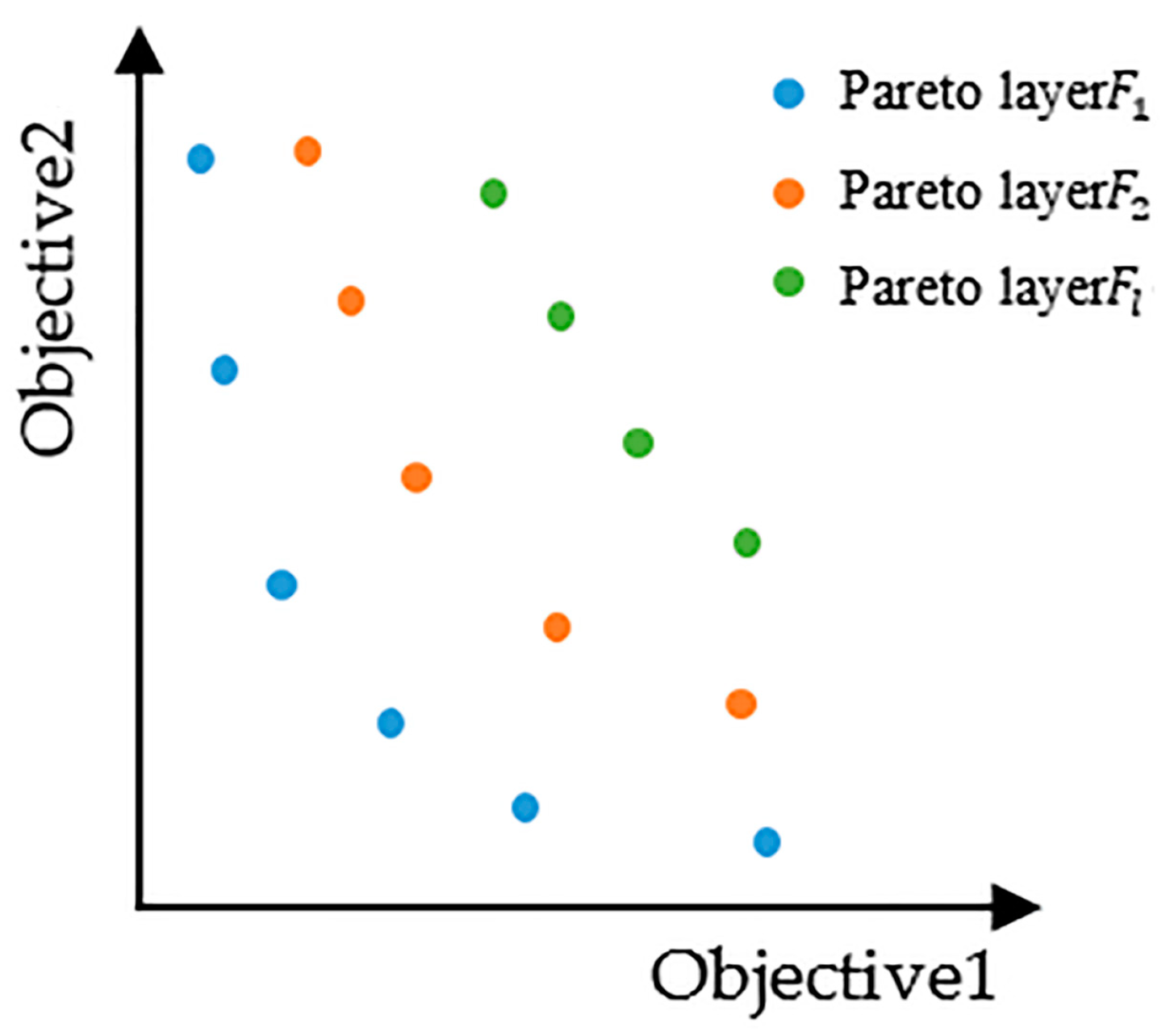$R_t$ undergoes a routine of fast non-dominated sorting and reference point distance sorting. Fast non-dominated sorting sorts individuals in $R_t$ into $l$ layers such as $F_1$, $F_2$, …, $F_l$, as shown in Figure 3, for two-objective optimization. Individuals in the same layer are non-dominated by each other; otherwise, for a minimum optimization problem, individuals in $F_2$ are dominated by individuals in $F_1$, i.e., individuals in $F_1$ dominate individuals in $F_2$.

After fast non-dominated sorting, individuals with lower non-dominated ranks are merged into $S_t$ until the size of $S_t$ is greater than or equal to N. If the size of $S_t$ is greater than N, $P_{t+1}=S_t$ and the procedure moves into the next generation. Otherwise, $P_{t+1}={\displaystyle {\cup }_{j=1}^{l-1}{F}_j}$ and $k$ individuals are selected from $F_l$, $k=N-\left|P_{t+1}\right|$.

Reference point distance sorting is performed on individuals in $F_l$ to determine which $k$ individuals are selected. Reference point distance sorting includes four sections: determination of reference points on a hyper-plane, adaptive normalization of population members, association operation and niche-preservation operation. Firstly, for a three-objective problem with four divisions, widely distributed reference points are chosen for each objective axis which are produced using Das and Dennis’s systematic approach [29]. These reference points are deemed ideally well distributed in space, and the size of population must be the same as the number of reference points. Secondly, as the objectives are always in different units, they are normalized. Each minimum for $M$ objective functions $Z_i^{\min }$ are found to get them translated into objectives $f_i^{\prime }(x)=f_i(x)-z_i^{\min }$. With $f_i^{\prime }(x)$, extreme points are calculated as:

$$ASF\left(x,w\right)={max}_{i=1}^M{f}_i^{\prime }\left(x\right)/w_i,x\in S_t$$

(4)

$$z^{i,maxargmi{n}_{s\in S_t}{A^{i^{i^{-6^i}}}}_j}$$

(5)

Then, $M$ extreme objective vectors $Z^{i,\max }$ are made to constitute a linear hyper-plane. With this hyper-plane, the intercept $a_i$ of extreme vectors on the i-th objective axis can be computed. Therefore, the objective functions can be normalized using the following equation:

$$f_i^n\left(x\right)=\frac{f_i^{\prime }\left(x\right)}{a_i-z_i^{min}\frac{f_i\left(x\right)-z_i^{min}}{a_i-z_i^{min}}}$$

(6)

After this normalization, the perpendicular distance of each individual in $S_t$ is calculated from each of the reference lines, which is joined by the reference point with the origin on the hyper-plane. Then, the reference point with the smallest distance is associated with the individual. The niche count of a reference point is calculated, except for the last-domination layer, i.e., $F_l$, and the niche count can be zero or more than one. Individuals associated with the reference point that has the lowest niche count should be preserved to ensure population diversity. The reference point with the lowest niche count is selected to find out whether this point is associated with the individuals in $F_l$. If not, another reference point is selected until at least one individual in $F_l$ is associated. If none of the individuals in $P_{t+1}$ are associated with the selected reference point, the individual with the minimum perpendicular distance in $F_l$ is selected; otherwise, a random individual in $F_l$ is selected since the population diversity has already been assured. The niche preservation operation stops once $k$ individuals are selected in $F_l$. As such, the size of $S_t$ is N, and the one loop of mutation, cross, non-dominated sorting and reference point distance sorting completes. This loop continues until the maximum generation or a stop criterion has been met.

A flow chart of the NSGA-III in parallel processing is presented in Figure 4.

3. Results

The altitude of LEO satellites drops quickly due to the dense atmosphere if no orbital maneuver happens [30]. Thus, the air drag effect on satellite orbital elements was first analyzed in order to roughly determine the altitude of a LEO constellation. Then, the optimal navigation constellation and augmentation constellation were designed. For a global navigation constellation, the two-objective functions are the GDOP and the number of satellites, while the decision variables are the number of satellites per plane, the number of planes and the corresponding inclination. The three- objective functions are the GDOP, the number of satellites and the satellite altitude, while the decision variables are the number of satellites per plane, the number of planes, the corresponding inclination and altitude. For a global augmentation constellation, the single-objective function is the global average of four, five and six visible satellites. The decision variables are the same as those of a navigation constellation but the range of satellites per plane and the number of planes differ because fewer satellites are needed for the augmentation system. A LEO augmentation constellation with the GNSS was designed and the GDOPs of the GNSS with and without a LEO constellation were compared. The time of serial computing and parallel computing for navigation were compared. An optimal constellation under each specific condition was obtained and recommended.

3.1. Air Drag Effects on LEO Satellites

Air drag effects on satellite orbital elements in 20 days at an altitude of 500 km~1100 km were analyzed using the Satellite Analysis Tool Kit (STK) software. The forces included the Earth’s gravitational field with zonal and tesseral harmonics up to degree 31 and order 31, ocean tides, solid tides, solar radiation pressure, Jacchia 1970 drag model and third-body gravity. The ratio of satellite area and mass was 0.01 m²/kg. The results listed in

Table 1. Drag effects on orbital elements in 20 days at an altitude of 500 km~1100 km.

Altitude (km)	Semi-Major Axis (m)	Eccentricity	Inclination (deg)	RAAN (deg)	Argument of Perigee (deg)	Mean Anomaly (deg)
500	8131.5	6.09 × 10−4	0.0162	0.0639	9.1467	359.9227
600	951.5	8.18 × 10−5	0.0018	0.0071	3.0328	359.7060
700	497.98	4.56 × 10−5	9.05 × 10−4	0.0037	1.5349	359.6837
800	157.03	1.37 × 10−5	2.74 × 10−4	0.0011	2.2769	10.8145
900	31.91	2.52 × 10−6	5.51 × 10−5	2.18 × 10−4	−0.1777	3.9658
1000	32.66	1.73 × 10−6	5.43 × 10−5	2.18 × 10−4	−0.2131	2.4606
1100	15.64	1.49 × 10−6	−3.78 × 10−5	1.14 × 10−4	0.0470	−0.0169

show that the drag force mainly had a significant effect on the semi-major axis, while the effects on the other elements were negligible. When a satellite was placed at a 500 km altitude, the semi-major axis decreased by 8 km in 20 days. Drag effects significantly decreased with an increase in satellite altitude. The semi-major axis decreased just 30 m in 20 days when the satellite altitude was 900 km, which is acceptable for LEO constellation maintenance. According to this simulation analysis, a LEO constellation is better placed above a 900 km altitude.

3.2. LEO Global Navigation Constellation Design

The altitude of a LEO satellite constellation is better when it is higher than 900 km and lower than 1500 km in order to avoid the radiation of the inner Van Allen radiation belt. Optimal constellations were designed every 100 km from 900 km to 1500 km. For the multi-objective optimization problem, the members were binary-coded. The decision variable ranges of two- and three-objective optimization are listed in

Table 2. Decision variable ranges of two- and three-objective optimization.

Optimization Cases	Range	S	P	Inclination (deg)	Altitude (km)
Two-objective	L	15	10	75	-
	U	30	15	105	-
Three-objective	L	15	10	75	900
	U	30	15	105	1500

. The inclination range of a near-polar constellation was randomly chosen from 75° to 105° in order to narrow down the search space. $S$ represents the number of satellites per plane, and $P$ represents the number of planes. The ranges of these two variables were randomly selected, which made the total number of satellites lie between 150 and 450. The variable numbers of bits of two- and three-objective optimization are listed in

Table 3. Number of bits in two- and three-objective optimization.

Optimization Cases	S	P	Inclination	Altitude
Two-objective	4	3	5	-
Three-objective	4	3	5	9

. Parameter settings are listed in

Table 4. Parameter settings.

Parameters	Max Generation	N	Crossover Probability	Mutation Probability
Number	100	100	0.9	1/n (n is number of variables)

.

The Earth’s surface is divided into 6° × 6° grids, which means that 1800 ground stations distributed symmetrically and evenly were used to estimate the GDOP of the designed satellite constellation. Master–slave parallel computing was used for time saving. A satellite was regarded as visible when the elevation angle was larger than 7°. The optimization process considered the Earth’s second zonal harmonic efficiency with a propagation interval of 60 s. For $P$ planes in a constellation, $P$ configurations were analyzed for the phase factor $F$ from $0$ to $P-1$. For a point $r_p$ on the earth surface at time $t$, the GDOP relative to constellation $c$ is expressed as $GDOP(r_p,t,c)$. The maximum GDOP of all the points in the orbital period $T_p$ of $P$ configurations is minimized, which can be denoted by a fitness function as

$$Fitnes{s}_1=\underset{t\in \left(0,T_P\right)}{max}\underset{F\in \left(0,P-1\right)}{max}\underset{r_{P\in }Earth}{max}GDOP\left(r_P,t,c\right)$$

(7)

The second fitness function is

$$Fitnes{s}_2=s\times p$$

(8)

The third fitness function is

$$Fitnes{s}_3=altitudes$$

(9)

The first and second fitness functions were used for a two-objective optimization; three fitness functions were used for a three-objective function optimization.

3.2.1. Two-Objective Optimization

The search results of two-objective optimization with altitudes ranging from 900 km to 1500 km are presented in Figure 5. The GDOP results lay between 1.36 and 5.13, and the number of satellites lay between 160 and 435. For altitudes of 900, 1000, 1100, 1200, 1300, 1400 and 1500 km, the number of satellites was greater than 264, 252, 210, 210, 200, 190 and 200, respectively, when the GDOP in the optimal sets was, first, smaller than three. Note that all the inclinations were around 90°. Fewer satellites were needed for a global average GDOP smaller than three at a higher altitude.

Among all the results, the following configurations are recommended after taking both the number of satellites and the GDOP into consideration: W264/12/1 with an inclination of 88.54° for the altitude of 900 km; W240/10/9 with an inclination of 85.64° for the altitude of 1000 km; W210/10/7 with an inclination of 85.64° for the altitude of 1100 km; W210/10/8 with an inclination of 85.64° for the altitude of 1200 km; W200/10/1 with an inclination of 86.72° for the altitude of 1300 km; W190/10/8 with an inclination of 88.55° for the altitude 1400 km; and W180/10/1 with an inclination of 85.64° for the altitude 1500 km. Satellites in space with these configurations are showed in Figure 6.

The global average of visible satellites and the GDOP of the above-mentioned configurations in 24 h are listed in

Table 5. Global average of visible satellites and geometric dilution of precision (GDOP) in 24 h.

Altitude (km)	Configuration	Inclination (deg)	Visible Satellites	GDOP
900	W264/12/1	88.54	14.55	2.36
1000	W240/10/9	85.64	14.49	2.80
1100	W210/10/7	85.64	13.83	2.47
1200	W210/10/8	85.64	14.96	1.87
1300	W200/10/1	86.72	15.32	1.69
1400	W190/10/8	88.55	15.57	2.51
1500	W180/10/1	85.64	15.55	2.81

. The global visible satellites and the GDOP with latitudes are shown in Figure 7. It can be seen that the average visible satellites of all the altitudes are between 5 and 35; the average GDOPs of 1200 km and 1300 km are between 0.5 and 3; the GDOPs of other cases are between 0.5 and 5. The visible satellites of high altitudes are more than those of low latitudes because the inclination is near 90°, and the minimum visible satellites at a low latitude are greater than five.

3.2.2. Three-Objective Optimization

The results of the three-objective optimization are presented in Figure 8. The number of satellites lay between 150 and 360, the GDOP between 1.4347 and 5.5911 and the altitude between 904.7058 km and 1476.4705 km. Taking the GDOP, the number of satellites and the altitude into consideration, the configuration of W 252/12/1 with an inclination of 85.64° and an altitude of 1008.23 km is recommended for the three-objective optimization. The constellation in space is shown in Figure 9. The average global visible satellites and the GDOP in 24 h were 18.31 and 1.54, respectively.

3.2.3. Calculation Time of Parallel and Serial Computing

Since the multi-objective optimization process is time-consuming, it is important to reduce the computation costs; for example, by a parallel computing technology. The running time of parallel and serial computing under two- and three-objective optimization conditions are calculated and presented in

Table 6. Time of serial and parallel computing with two-objective optimization at 1400 km altitude (in hours).

Optimization Cases	Serial Computing	Parallel Computing
Two-objective	125.2513	4.5805
Three-objective	115.1403	4.0883

. Parallel computing is achieved with 60 computer cluster cores. For two-objective optimization with an altitude of 1400 km, serial computing requires 125.2513 h, while the parallel computing requires only 4.5805 h, making it 27.3 times faster than serial computing. For the three-objective optimization condition, parallel computing runs at 4.0083 h, which is 28.16 times faster than serial computing.

3.3. LEO Global Augmentated Constellation Design

The decision variable ranges of one constellation and a hybrid constellation for augmentation are listed in

Table 7. Decision variable ranges.

Constellation Types		Range	S	P	Inclination (deg)	Altitude (km)
Walker		L	4	4	75	-
		U	15	15	105	-
Walker/Walker	Walker1	L	4	4	0	900
		U	12	12	45
	Walker2	L	4	4	45	1200
		U	12	12	90

. For one Walker constellation, the constellation was designed every 100 km from altitudes of 900 km to 1500 km. For a Walker/Walker hybrid constellation, altitudes were selected as 900 km and 1200 km. The decision variable ranges and the variable number of bits are listed in Table 7 and

Table 8. Number of variable bits.

Constellation Types	S	P	Inclination
Walker	4	4	5
Walker/Walker	3	3	6

, respectively. Parameter settings were the same as those of a navigation constellation.

The fitness function of the global average of visible satellites is

$$Fitnes{s}_4=\left|X-\delta \right|$$

(10)

where X is the global average of visible satellites, δ is set as four, five and six, respectively.

3.3.1. Walker Constellation

Configurations of W72/8/1, W91/7/2 and W108/9/1 were the search results for the global average of visible satellites of four, five and six at an altitude of 900 km, respectively. Globally visible satellites and the average visible satellites with altitudes of these three configurations are presented in Figure 10. The space configurations of these constellations are shown in Figure 11. For global average visible satellites of four, visible satellites were 1~3 for latitudes of 60°N~60°S. Among the other latitudes, visible satellites were larger than four, which meant constellation at these areas was able to provide PNT services. For a global average of five visible satellites, areas of visible satellites between 1~3 were less than the global average of four visible satellites. For a global average of six visible satellites, visible satellites of 13 were achieved at high latitudes, and the visible satellites of almost half the areas were between 4~10. More satellites were always viewed at higher latitudes because of a near-polar configuration, and uneven coverage was attained with only one Walker constellation.

The available percentages for navigation and average GDOP for four, five and six globally visible satellites are listed in

Table 9. Available percentage and GDOP in 24 h for four average visible satellites.

Altitude (km)	Configuration	Inclination (deg)	Available Percentage (%)	GDOP
900	W72/8/1	89.51	38.51	19.73
1000	W65/13/2	92.42	40.04	57.06
1100	W63/9/2	79.84	44.65	23.38
1200	W56/4/1	94.35	52.76	9.10
1300	W52/4/1	94.35	52.18	7.76
1400	W50/10/3	96.29	44.77	39.85
1500	W48/12/7	80.81	56.01	29.56

,

Table 10. Available percentage and GDOP in 24 h for five average visible satellites.

Altitude (km)	Configuration	Inclination (deg)	Available Percentage (%)	GDOP
900	W91/7/2	94.35	51.54	29.67
1000	W84/12/2	81.77	53.83	82.43
1100	W77/11/2	82.74	50.62	105.94
1200	W70/14/5	93.39	54.99	17.09
1300	W66/11/1	96.29	58.49	22.63
1400	W60/4/1	83.71	56.87	7.96
1500	W56/4/3	93.39	58.46	4.71

and

Table 11. Available percentage and GDOP in 24 h for six average visible satellites.

Altitude (km)	Configuration	Inclination (deg)	Available Percentage (%)	GDOP
900	W108/9/1	85.64	63.93	13.53
1000	W100/10/2	95.32	70.17	26.09
1100	W91/7/1	89.52	69.47	8.59
1200	W90/10/2	104.03	76.10	25.74
1300	W78/6/5	87.58	70.86	5.10
1400	W75/15/14	81.77	68.27	24.68
1500	W70/7/2	84.68	69.02	11.84

, respectively. The available percentage of navigation refers to the percentage of visible satellites that were greater than or equal to four in 24 h. Much fewer satellites were required for a global augmentation system than that of the navigation system. For a global average of four visible satellites, constellations at 1000 km/1200 km/1300 km/1400 km were retrograde orbits, and the constellation at 1300 km got the smallest average GDOP of 7.76. For a global average of five visible satellites, constellations at 900 km/1200 km/1300 km/1500 km were retrograde orbits, and the average GDOP of the constellation at 1500 km was less than five. For a global average of six visible satellites, constellations at 1000 km/1200 km were retrograde orbits, and the average GDOP of the constellation at 1300 km got the smallest GDOP of 5.10. With the global average of visible satellites increasing from four to five and six, the available percentages of navigation rose from approximately 40% to 50% and 60%, respectively.

3.3.2. Walker/Walker Constellation

The augmentation constellations described above were able to achieve global averages of four, five and six visible satellites. However, the visible satellites were uneven due to the near-polar configuration. To achieve a more even global coverage, a hybrid constellation constructed with two Walker constellations was designed. The inclination of one constellation was set between 0° and 45°, and the altitude was 900 km; the inclination of the other constellation was set between 45° and 90°, and the altitude was 1200 km. The globally visible satellites and the average visible satellites with latitudes for an average of four, five and six visible satellites are presented in Figure 12. With two constellations, a much more even coverage was obtained. The space configurations and parameters of these three hybrid configurations are listed in Figure 13 and

Table 12. Available percentage and GDOP in 24 h.

Average Visible Satellites	Altitude (km)	Configuration	Inclination (deg)	Available Percentage (%)	GDOP
4	900	W56/8/4	42.85	67.71	52.21
	1200	W32/8/2	87.59
5	900	W81/9/1	36.42	88.15	39.44
	1200	W40/10/1	85.0
6	900	W64/8/4	37.85	95.58	12.81
	1200	W60/10/4	87.85

, respectively. For a global average of six visible satellites, the percentage of this hybrid constellation capable of providing PNT services was 95.58%, and the global average GDOP was 12.81.

3.3.3. Walker/Walker Constellation with GNSS

The results in Section 3.3.1 and Section 3.3.2 are solely based on LEO satellites with the figure of merit of global visible satellites. However, as the GNSS is the mainstream of the PNT, the GDOPs of the GNSS with and without LEO satellites are worth studying. In this section, with the four GNSSs, an optimal LEO Walker/Walker constellation was designed using the NSGA-III, based on two objectives: GNSS/LEO GDOP and number of LEO satellites, i.e., $Fitnes{s}_1$ and $Fitnes{s}_2$. The decision variables of the LEO satellites were the same as those in Section 3.3.2 The satellite parameters of GPS, BDS, Galileo and GLONASS were based on documents [31,32,33,34], respectively. Without a LEO constellation, the maximum, mean and minimum GDOP of GNSS in 24 h are presented in Figure 14. The space configuration of GNSS is shown in Figure 15.

From the search results of the LEO constellation, the maximum, mean and minimum GDOPs of the GNSS/LEO in 24 h are presented in Figure 16. The space configuration of the GNSS/LEO is shown in Figure 17. The parameters of the LEO Walker/Walker constellation are displayed in

Table 13. Parameters of LEO Walker/Walker constellation.

Altitude (km)	Configuration	Inclination (deg)
900	W16/4/1	34.28
1200	W40/5/1	70

.

With 56 LEO satellites introduced in the GNSS, the mean GDOP of the GNSS with latitude decreased from 0.8882~1.0325 to 0.6438~0.8743, the maximum GDOP of the GNSS with latitude decreased from 1.1695~1.6264 to 1.0361~1.5611 and the minimum GDOP of the GNSS with latitude decreased from 0.6880~0.8670 to 0.4962~0.5533. The global mean GDOP of the GNSS decreased from 0.9549 to 0.8048; the global maximum GDOP of the GNSS decreased from 1.6264 to 1.5611 and the global minimum GDOP of the GNSS decreased from 0.6880 to 0.4962. Moreover, we arrived at the conclusion from the search process that the GDOPs of the GNSS could only decrease by a very small range even when more LEO satellites were introduced.

4. Conclusions

The premise of a LEO navigation system or a LEO-augmented GNSS system is a well-distributed global coverage LEO constellation. For a LEO-based navigation constellation, the GDOP and the number of satellites need to be considered. For a LEO-based global augmentation constellation, the global average of visible satellites is required. With one Walker configuration, it was hard to get even global coverage. Therefore, a hybrid Walker/Walker constellation was designed. The GDOPs of the GNSS with and without LEO satellites were compared.

To achieve a suitable altitude for the LEO constellation, the air drag effects on satellites at altitudes of 500 km to 1100 km were evaluated. The results showed that air drag had a great effect mainly on the semi-major axes of the satellites, whose altitudes were lower than 900 km. For satellites with an altitude of 500 km, the semi-major axis decreased by 8 km in 20 days. The semi-major axis decreased by 31 meters for satellites with an altitude of 900 km.

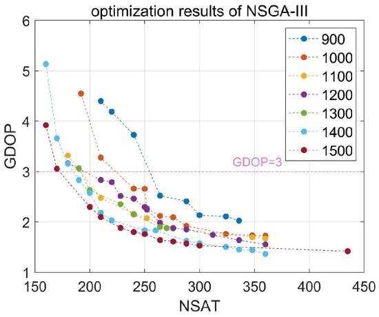
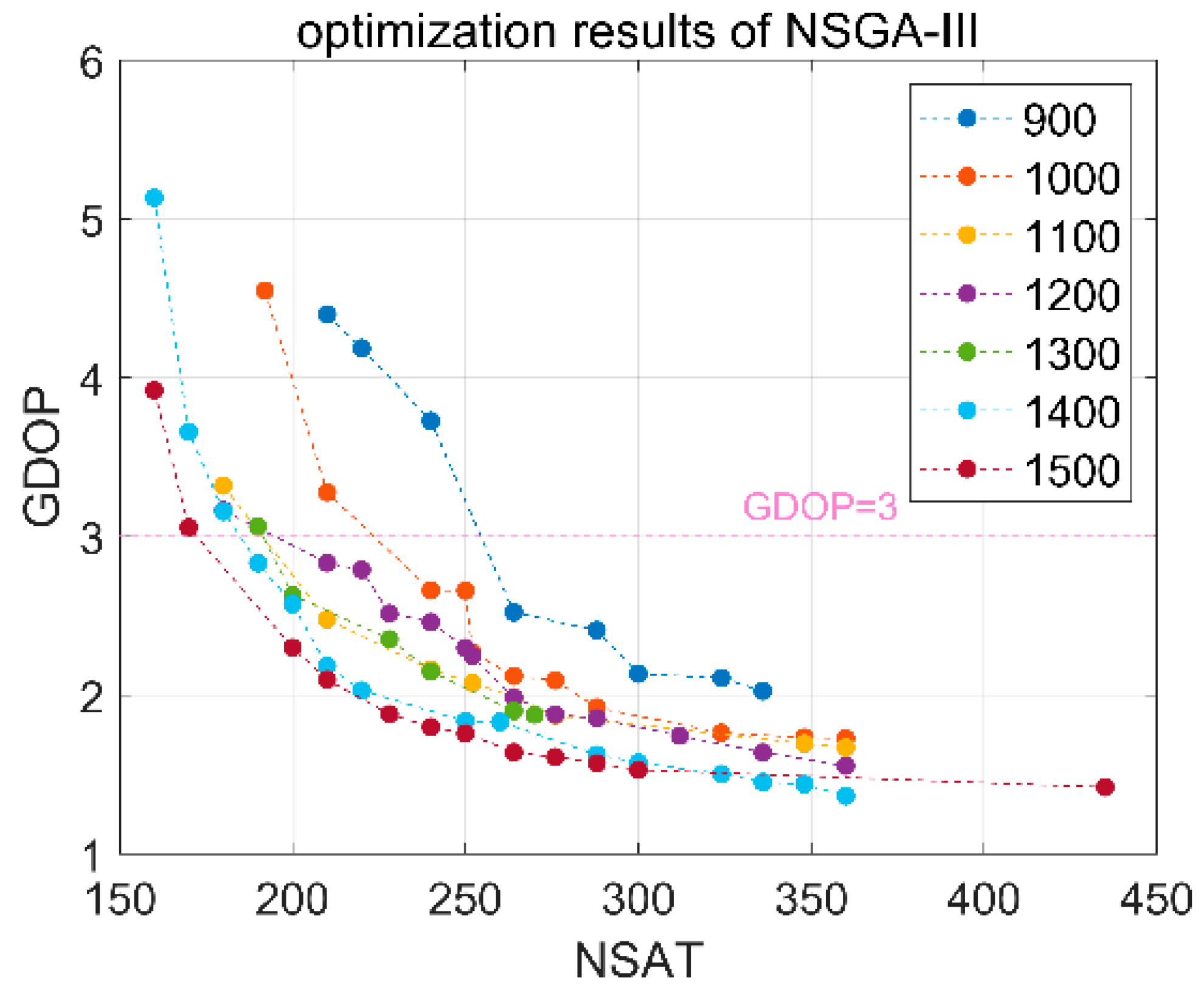
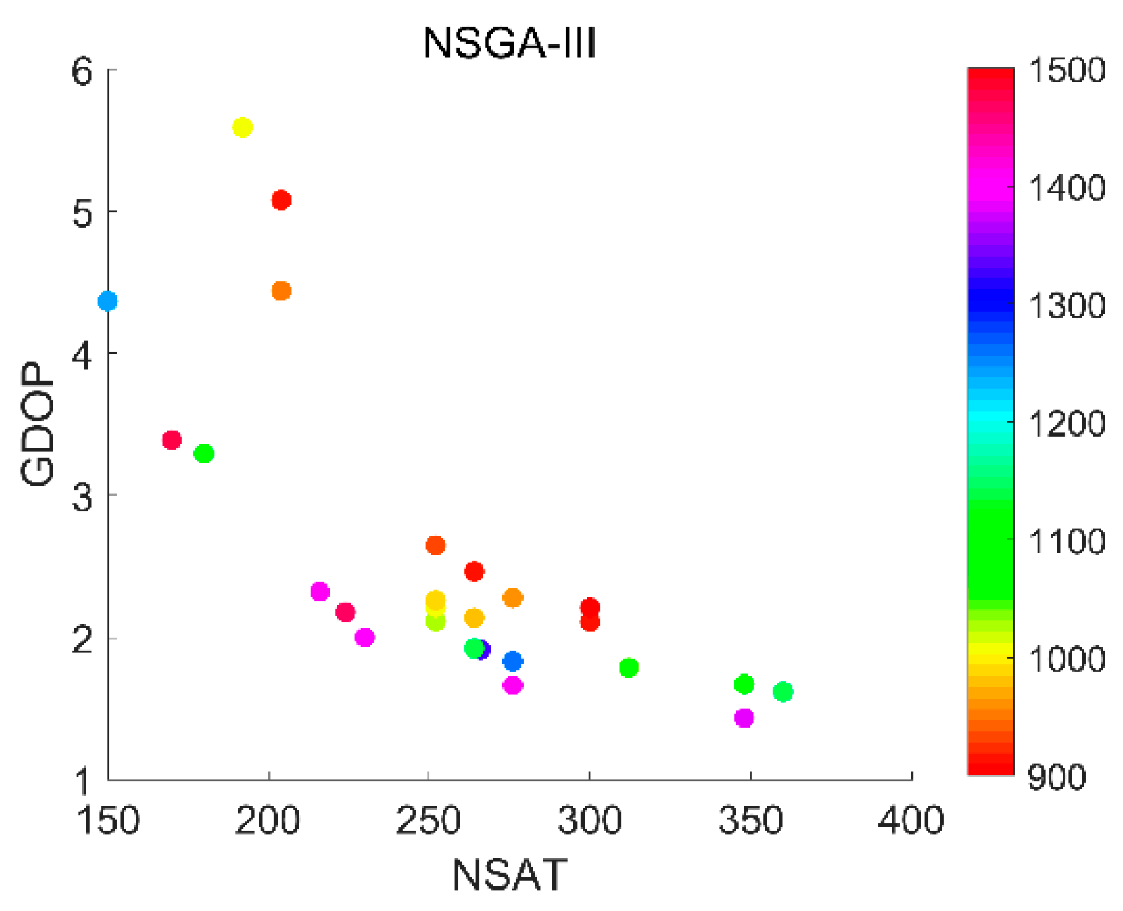
With a suitable altitude range, global navigation constellations were designed with two-objective and three-objective optimization. The results demonstrate that the following configurations are recommended for two-objective optimization: for an altitude of 900 km, the configuration of W264/12/1 with an inclination of 88.54°; for an altitude of 1000 km, W240/10/9 with an inclination of 85.64°; for an altitude of 1100 km, W210/10/7 with an inclination of 85.64°; for an altitude of 1200 km, W210/10/8 with an inclination of 85.64°; for an altitude of 1300 km, W200/10/1 with an inclination of 86.72°; for an altitude of 1400 km, W190/10/8 with an inclination of 88.55°; and for an altitude of 1500 km, W180/10/1 with an inclination of 85.64°. For global navigation with three-objective optimization, a configuration of W252/12/1 with an inclination of 85.64° and altitude of 1008.23 km is recommended.

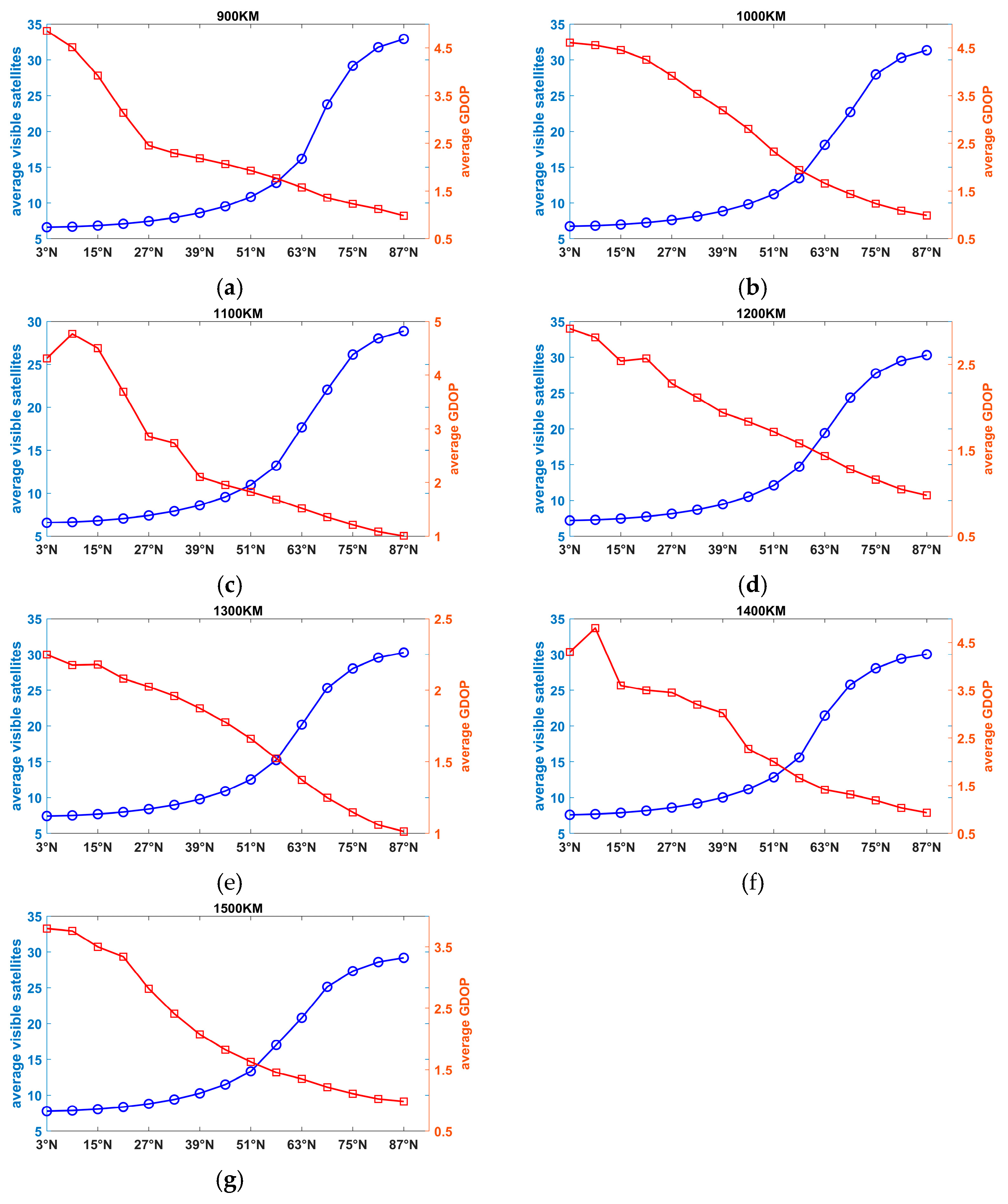
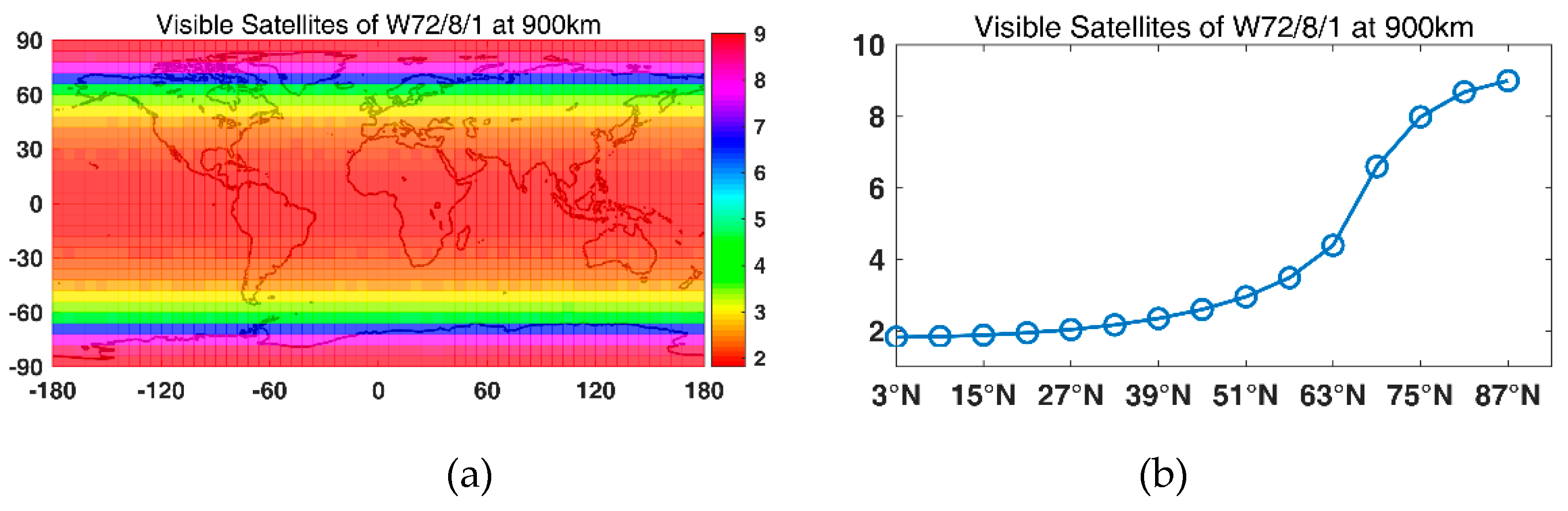
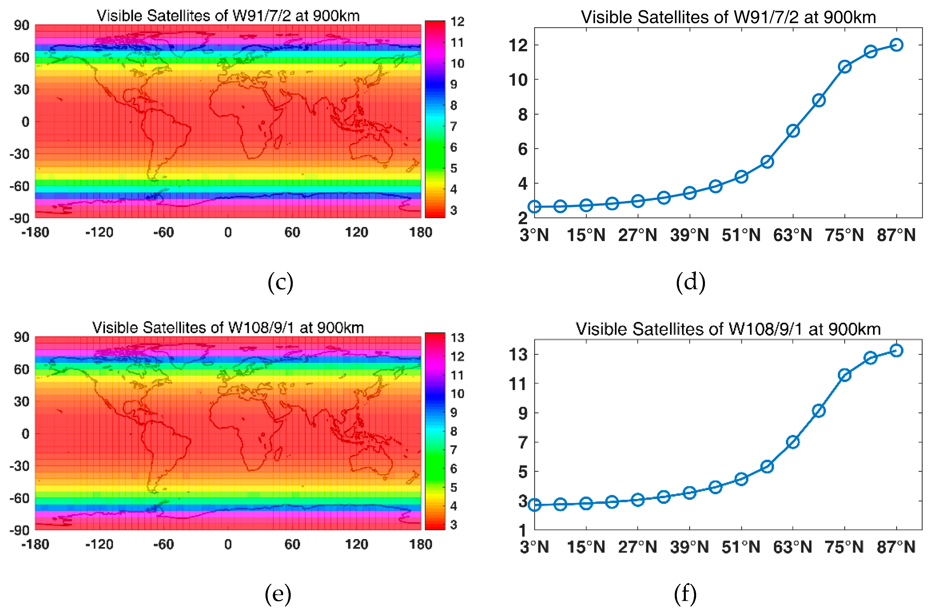
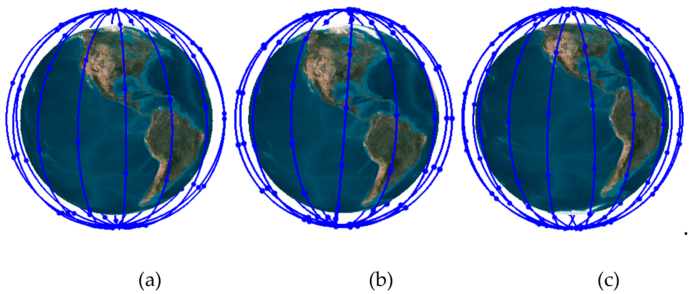
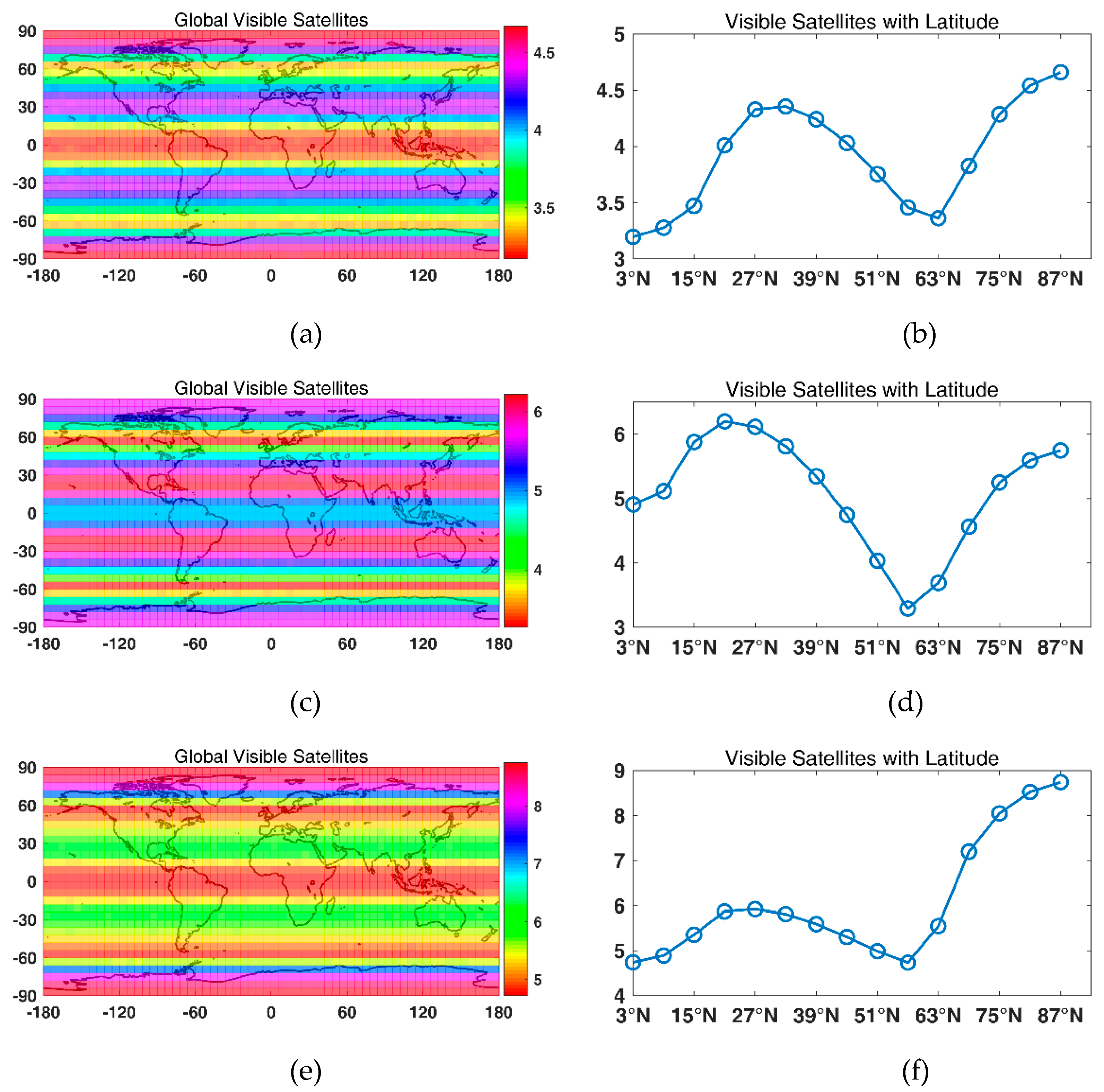
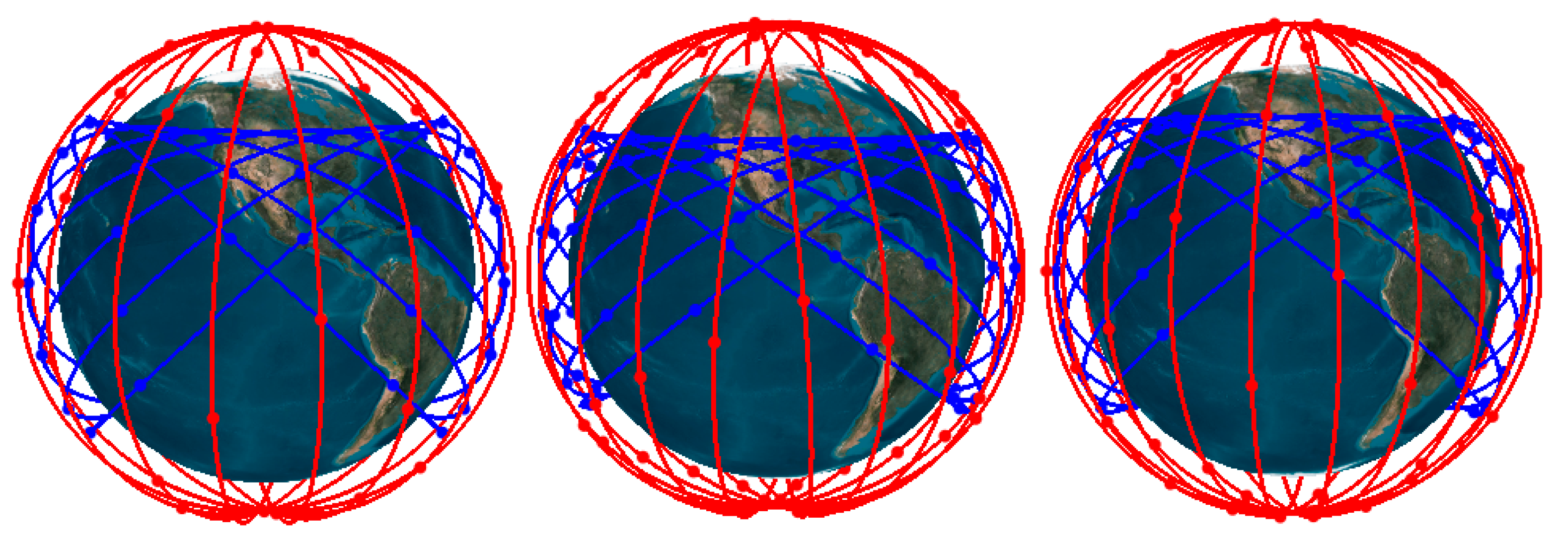
Then, LEO-based augmentation constellations were designed using the GA. First, a constellation with one Walker constellation was designed. For a global average of four visible satellites, 72/65/63/56/52/50/48 satellites were needed for altitudes of 900 km/1000 km/1100 km/1200 km/1300 km/1400 km/ and 1500 km, respectively. For a global average of five visible satellites, 91/84/77/70/66/60/56 satellites were needed for altitudes of 900 km/1000 km/1100 km/1200 km/1300 km/1400 km/ and 1500 km, respectively. For a global average of six visible satellites, 108/100/91/90/78/75/70 satellites were needed for altitudes of 900 km/1000 km/1100 km/1200 km/1300 km/1400 km/ and 1500 km, respectively. With the global average of visible satellites increasing from four to five and six, the available percentage for navigation increased approximately from 40% to 50% and 60%. Note that it was hard to achieve even global coverage with one constellation. Therefore, a Walker/Walker hybrid constellation was designed. The results show that a more even global coverage could be achieved with two constellations, and the available percentage of navigation of an average of six visible satellites was 95.58%.

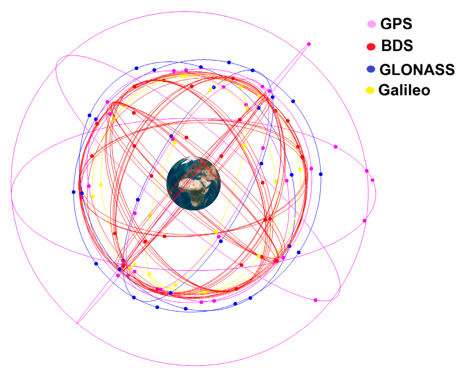
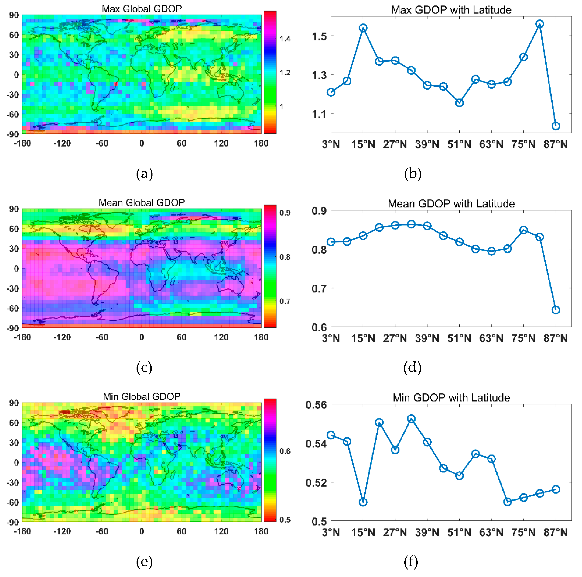
A hybrid Walker/Walker LEO constellation along with GNSS satellites was designed using the NSGA-III with two-objective optimization. The results show that with the 56 LEO satellites introduced in the GNSS, the global mean GDOP of the GNSS decreased from 0.9549 to 0.8048; the global maximum GDOP of the GNSS decreased from 1.6264 to 1.5611; and the global minimum GDOP of the GNSS decreased from 0.6880 to 0.4962. Note that even though only a small range of GDOP was improved, the main contribution of LEO satellites was to reduce the convergence time of the GNSS PPP and provide a backup PNT service where GNSS signals were blocked or interfered with.

The results above were obtained by using NSGA-III and GA. It can be seen that the NSGA-III was able to find the optimal front of constellation design. Parallel computing shortens the running time considerably. With parallel computing, the NSGA-III under a 1400 km altitude and three-objective optimization runs 27.3 and 28.16 times faster, respectively, than serial computing.

In summary, LEO-based navigation constellations with a Walker configuration need 180~264 satellites for altitudes of 1500 km~900 km in order to achieve a global average GDOP of less than three; LEO-based augmentation constellations with a Walker configuration need fewer satellites than navigation constellation to realize global averages of four, five and six visible satellites. Nevertheless, due to the constraint of global coverage, LEO-based augmentation constellations with a single Walker configuration find it hard to achieve even global even coverage. Instead of a single Walker configuration, a hybrid Walker/Walker constellation is able to achieve a more even global coverage.

References

1. China Satellite Navigation Office. Development of the BeiDou Navigation Satellite System; (Version 4.0); China Satellite Navigation Office: Beijing, China, 2019. [Google Scholar]
2. Reid, T. Orbital Diversity for Global Navigation Satellite Systems. Ph.D. Thesis, Stanford University, Stanford, CA, USA, 2017. [Google Scholar]
3. David Lawrence, H.S. Innovation: Navigation from LEO 2017. Available online: https://www.gpsworld.com/innovation-navigation-from-leo/ (accessed on 30 June 2017).
4. Li, X.; Ma, F.; Li, X.; Lv, H.; Bian, L.; Jiang, Z.; Zhang, X. LEO constellation-augmented multi-GNSS for rapid PPP convergence. J. Geodesy 2019, 93, 749–764. [Google Scholar] [CrossRef]
5. Li, X.; Zhang, K.; Ma, F.; Zhang, W.; Zhang, Q.; Qin, Y.; Zhang, H.; Meng, Y.; Bian, L. Integrated Precise Orbit Determination of Multi-GNSS and Large LEO Constellations. Remote. Sens. 2019, 11, 2514. [Google Scholar] [CrossRef] [Green Version]
6. Su, M.; Su, X.; Zhao, Q.; Liu, J. BeiDou Augmented Navigation from Low Earth Orbit Satellites. Sensors 2019, 19, 198. [Google Scholar] [CrossRef] [PubMed] [Green Version]
7. Mazouffre, S. Electric propulsion for satellites and spacecraft: Established technologies and novel approaches. Plasma Sources Sci. Technol. 2016, 25, 033002. [Google Scholar] [CrossRef]
8. Levchenko, I.; Xu, S.; Mazouffre, S.; Lev, D.; Pedrini, D.; Goebel, D.; Garrigues, L.; Taccogna, F.; Bazaka, K. Perspectives, frontiers, and new horizons for plasma-based space electric propulsion. Phys. Plasmas 2020, 27, 020601. [Google Scholar] [CrossRef] [Green Version]
9. Lemmer, K. Propulsion for cubesats. Acta Astronaut. 2017, 134, 231–243. [Google Scholar] [CrossRef]
10. Djebko, K.; Puppe, F.; Kayal, H. Model-Based Fault Detection and Diagnosis for Spacecraft with an Application for the SONATE Triple Cube Nano-Satellite. Aerospace 2019, 6, 105. [Google Scholar] [CrossRef] [Green Version]
11. Reid, T.G.; Neish, A.M.; Walter, T.F.; Enge, P.K. (Eds.) Leveraging commercial broadband LEO constellations for navigation. In Proceedings of the ION GNSS Conference, Portland, Oregon, 12–16 September 2016. [Google Scholar]
12. Portillo, I.D.; Cameron, B.G.; Crawley, E.F. A technical comparison of three low earth orbit satellite constellation systems to provide global broadband. Acta Astronaut. 2019, 159, 123–135. [Google Scholar] [CrossRef]
13. Meng, Y.; Bian, L.; Han, L.; Lei, W.; Yan, T.; He, M.; Li, X. (Eds.) A global navigation augmentation system based on LEO communication constellation. In Proceedings of the 2018 European Navigation Conference (ENC), Gothenburg, Sweden, 14–17 May 2018. [Google Scholar]
14. Walker, J.G. Satellite constellations. J. Br. Interplanet. Soc. 1984, 37, 559–572. [Google Scholar]
15. Luders, R.D. Satellite networks for continuous zonal coverage. ARS J. 1961, 31, 179–184. [Google Scholar] [CrossRef]
16. Mortari, D.; Wilkins, M.P.; Bruccoleri, C. The flower constellations. J. Astronaut. Sci. 2004, 52, 107–127. [Google Scholar]
17. Ely, T.; Crossley, W.; Williams, E. Satellite constellation design for zonal coverage using genetic algorithms. J. Astronaut. Sci. 1999, 47, 207–228. [Google Scholar]
18. Ferringer, M.P.; Clifton, R.S.; Thompson, T.G. Efficient and accurate evolutionary multi-objective optimization paradigms for satellite constellation design. J. Spacecr. Rocket. 2007, 44, 682–691. [Google Scholar] [CrossRef]
19. Ferringer, M.P.; Spencer, D.B. Satellite constellation design tradeoffs using multiple-objective evolutionary computation. J. Spacecr. Rocket. 2006, 43, 1404–1411. [Google Scholar]
20. Lang, T. (Ed.) Low Earth orbit satellite constellations for continuous coverage of the mid-latitudes. In Proceedings of the AIAA/ AAS Astrodynamics Specialist Conference, San Diego, CA, USA, 29–31 July 1996. AIAA-96-3638-CP paper. [Google Scholar]
21. Zhang, T.-J.; Shen, H.-X.; Li, Z.; Qie, H.; Cao, J.; Li, H.-N.; Yang, Y.-K. Restricted constellation design for regional navigation augmentation. Acta Astronaut. 2018, 150, 231–239. [Google Scholar] [CrossRef]
22. Shtark, T.; Gurfil, P. Regional positioning using a low Earth orbit satellite constellation. Celest. Mech. Dyn. Astron. 2018, 130, 14. [Google Scholar] [CrossRef]
23. Ma, F.; Zhang, X.; Li, X.; Cheng, J.; Guo, F.; Hu, J.; Pan, L. Hybrid constellation design using a genetic algorithm for a LEO-based navigation augmentation system. GPS Solut. 2020, 24, 1–14. [Google Scholar] [CrossRef]
24. Xia, Y.; Li, J. Inter-satellite links analysis of walker constellite. J. Geod. Geodyn. 2012, 32, 143–147. [Google Scholar]
25. Kaplan, E.; Hegarty, C. Understanding GPS: Principles and Applications; Artech House: Boston, MA, USA; London, UK, 2005. [Google Scholar]
26. Deb, K.; Jain, H. An evolutionary many-objective optimization algorithm using reference-point-based nondominated sorting approach, part I: Solving problems with box constraints. IEEE Trans. Evol. Comput. 2013, 18, 577–601. [Google Scholar] [CrossRef]
27. Deb, K.; Pratap, A.; Agarwal, S.; Meyarivan, T. A fast and elitist multiobjective genetic algorithm: NSGA-II. IEEE Trans. Evol. Comput. 2002, 6, 182–197. [Google Scholar] [CrossRef] [Green Version]
28. Ishibuchi, H.; Imada, R.; Setoguchi, Y.; Nojima, Y. (Eds.) Performance comparison of NSGA-II and NSGA-III on Various Many-Objective Test Problems. In Proceedings of the 2016 IEEE Congress on Evolutionary Computation (CEC), Vancouver, BC, Canada, 24–29 July 2016. [Google Scholar]
29. Das, I.; Dennis, J.E. Normal-Boundary Intersection: A New Method for Generating the Pareto Surface in Nonlinear Multicriteria Optimization Problems. Siam J. Optim. 1998, 8, 631–657. [Google Scholar] [CrossRef] [Green Version]
30. Montenbruck, O.; Gill, E.; Lutze, F. Satellite orbits: Models, methods, and applications. Appl. Mech. Rev. 2002, 55, B8–B27. [Google Scholar] [CrossRef]
31. Department of Deefense, U.S.A. Global Positioning System Standard Positioning Service Performance Standard, Gps Its Augment. System 2020. [Google Scholar] [CrossRef]
32. BeiDou, I. BeiDou Navigation Satellite System Signal in Space Interface Control Document Open Service Signal B1I (Version 3.0); China Satellite Navigation Office: Beijing, China, 2012.
33. Galileo, I. European GNSS (Galileo) Open Service Signal In Space Interface Control Document; (OS SIS ICD) European Space Agency/European GNSS Supervisory Authority: Brussels, Belgium, 2015. [Google Scholar]
34. GLONASS I. Global Navigation Satellite System GLONASS, Interface Control Document, Navigational Radio Signal in bands L1, L2; Russian Institute of Space Device Engineering: Moscow, Russia, 2008. [Google Scholar]
Figure 1. Footprints of LEO (low Earth orbit) satellite versus MEO (medium Earth orbit) satellite.
Remotesensing 12 01845 g001
Figure 2. Iridium constellation.
Remotesensing 12 01845 g002
Figure 3. Non-dominated sorting.
Remotesensing 12 01845 g003
Figure 4. Flow chart of non-dominated sorting genetic algorithm III (NSGA-III) in parallel processing.
Remotesensing 12 01845 g004
Figure 5. Optimization results of two-objective optimization.
Remotesensing 12 01845 g005
Figure 6. Optimal configurations of a two-objective optimization: (a) W264/12/1 for the altitude of 900 km; (b) W240/10/9 for the altitude of 1000 km; (c) W210/10/7 for the altitude of 1100 km; (d) W210/10/8 for the altitude of 1200 km; (e) W200/10/1 for the altitude of 1300 km; (f) W190/10/8 for the altitude of 1400 km; (g) W180/10/1 for the altitude of 1500 km.
Remotesensing 12 01845 g006
Figure 7. Average visible satellites and GDOPs of optimization configurations: (a) W264/12/1 for the altitude of 900 km; (b) W240/10/9 for the altitude of 1000 km; (c) W210/10/7 for the altitude of 1100 km; (d) W210/10/8 for the altitude of 1200 km; (e) W200/10/1 for the altitude of 1300 km; (f) W190/10/8 for the altitude of 1400 km; (g) W180/10/1 for the altitude of 1500 km.
Remotesensing 12 01845 g007
Figure 8. Optimization results of three-objective optimization.
Remotesensing 12 01845 g008
Figure 9. Optimal configurations of three-objective optimization.
Remotesensing 12 01845 g009
Figure 10. Visible satellites: (a) Global visible satellites of W72/8/1; (b) Visible satellites with latitude of W72/8/1; (c) Global visible satellites of W91/7/2; (d) Visible satellites with latitude of W91/7/2; (e) Global visible satellites of W108/9/1; (f) Visible satellites with latitude of W108/9/1.
Remotesensing 12 01845 g010aRemotesensing 12 01845 g010b
Figure 11. Constellations for average of four, five and six visible satellites: (a) W72/8/1; (b) W91/7/2; (c) W108/9/1.
Remotesensing 12 01845 g011
Figure 12. Visible satellites: (a) Global visible satellites for average visible satellites of four; (b) Visible satellites with latitude for average of four visible satellites; (c) Global visible satellites for average of five visible satellites; (d) Visible satellites with latitude for average of five visible satellites; (e) Global visible satellites for average of six visible satellites; (f) Visible satellites with latitude for average of six visible satellites.
Remotesensing 12 01845 g012
Figure 13. Space configurations: (a) Average visible satellites of four; (b) Average visible satellites of five; (c) Average visible satellites of six.
Remotesensing 12 01845 g013
Figure 14. GDOP of global navigation satellite system (GNSS) in 24 h: (a) Maximum global GDOP; (b) Maximum GDOP with latitude; (c) Mean global GDOP; (d) Mean GDOP with latitude; (e) Minimum global GDOP; (f) Minimum GDOP with latitude.
Remotesensing 12 01845 g014
Figure 15. Space configuration of GNSS.
Remotesensing 12 01845 g015
Figure 16. GDOP of GNSS/LEO in 24 h: (a) Maximum global GDOP; (b) Maximum GDOP with latitude; (c) Mean global GDOP; (d) Mean GDOP with latitude; (e) Minimum global GDOP; (f) Minimum GDOP with latitude.
Remotesensing 12 01845 g016
Figure 17. Space configuration of GNSS/LEO.
Remotesensing 12 01845 g017