1. Introduction
Providing high precision satellite orbit and clock products are key to precise point position (PPP) [
1,
2,
3]. As is well known, GLONASS satellites transmit signals through the frequency division multiple access (FDMA) technique, which leads to inter-channel biases and presents a challenge to GLONASS satellite clock offset estimation. For GLONASS, both pseudo-range and carrier-phase observations are influenced by inter-channel biases (ICBs). Carrier-phase ICBs ideally show linear dependence on frequency and can be fully absorbed by ambiguity parameters [
4,
5,
6,
7,
8,
9]. However, pseudo-range ICB does not share these characteristics and may degrade PPP performance if left unmanaged [
10,
11,
12]. GPS observations, particularly the code, can be affected by pseudo-range ICB-like biases as well, because the signals of GPS satellites are susceptible to individual chip shape distortions, even when the design is identical. These signal deformations cause different correlator tracking point shifts, giving rise to different receiver-related and channel-specific pseudo-range biases for each satellite [
13]. Consequently, the traditional method adopted in geodetic processing, which separates biases into purely receiver-dependent and purely satellite-dependent parts, is not always valid and thus requires further refinement [
14]. This motivates us to investigate in this work the necessity of accounting for the possible presence of GPS-ICB when estimating GPS satellite clock offsets.
Certain studies have revealed that the GLONASS ICBs estimated using short baseline data can reach up to several meters [
4,
8,
11,
15]. Several researchers have modeled these ICBs as linear functions of frequency to reduce the effect on positioning [
11,
16,
17], but this linearity may not hold true in all cases. Considering the experiences we obtained in the GLONASS case, we extend this to the GPS case with GPS-ICBs in this study. The former works were focused mainly on the characteristics of GPS pseudo-range ICBs [
14,
18], but barely on their effects on PPP and satellite clock offset estimation, which constitute the main contribution of this work.
For this study, four GLONASS ICB schemes considered for GLONASS clock offset estimation are presented below. Thereafter, data processing strategies are introduced. The details of the ICB characteristics and analyses of the corresponding effects on GLONASS satellite clock offset estimation and PPP are presented next. Considering the chip shapes of GPS signals, the introduction of an ICB parameter into the GPS observation equation is described to analyses of the pseudo-range ICB characteristics and effects on GPS satellite clock offset estimation and PPP. Finally, the results and corresponding conclusions are summarized.
2. Method of Satellite Clock Offset Estimation
The equations for the un-differenced pseudo-range and carrier phase can be expressed as follows:
here,
is the pseudo-range observation, where the subscript
refers to the receiver and the superscript
denotes the satellite;
is the epoch number;
is the geometric distance between the receiver and satellite phase center;
is the tropospheric delay;
denotes the frequency-dependent factor;
is the ionosphere delay on band 1;
is the speed of light in vacuum;
and
are the receiver and satellite clock offset, respectively [
19,
20];
is the original phase measurement in cycles, and
is the carrier phase observation in meters;
and
are the receiver and satellite hardware delays for the pseudo-range, respectively;
is the frequency number;
and
are the carrier phase uncalibrated fractional carrier phase offsets for the receiver and satellite, respectively [
21,
22,
23];
is the signal wavelength;
is the carrier phase ambiguity; and
and
are the noises and other un-modeled errors e.g., multipath effects of code and phase observations, respectively.
Generally, for GNSS satellite clock offset estimation, the ionosphere-free (IF) linear combination is used to eliminate the first-order ionospheric effect. Therefore, the combination of observations can be expressed as follows:
The delays
and
in (3) are considered to be constants during daily processing in accordance with international GNSS service (IGS) practice [
24,
25]. Furthermore, the absolute values of
and
cannot be determined separately or considered to be known. Therefore, expression (3) can be reparametrized to eliminate the rank defect, yielding the redefined receiver and satellite clock offset
and
in (4) [
26]. By integrating the correlated parameters, the following equations can be obtained:
The equation with the ICB for GLONASS can be formulated as follows:
As shown in (6), the receiver clock offset
is highly correlated with the satellite clock offset
, which leads to a rank defect in the normal equation matrix. To eliminate the correlation, one clock datum should be chosen to estimate the clock offset with respect to the datum [
27,
28,
29]. Then, the group receiver clock offset in the network can be selected as a reference according to the following strategy:
where
is the number of stations,
denotes the estimated receiver clock offset, and
represents the approximate values of the receiver clock offset, which are obtained from single point positioning (SPP).
To introduce the ICBs, we tested four different strategies to constrain the ICB parameters.
In the first strategy, no ICB parameters are used for the estimation. Then, the expression of clock offset estimation for GLONASS is simply (4). Here, we refer to this model as ICB-NONE.
In the second approach, common bias parameters for GLONASS satellites are assumed. The ICBs are set as quadratic polynomial function of the frequency number. Thus, the ICBs can be modeled as
where
is the frequency number of a GLONASS satellite, which varies from −7 to 6;
denotes the ICBs for a GLONASS satellite with frequency number 0; and
and
are the newly defined ICB coefficient that are linearly and quadratically dependent on the frequency number, respectively. The sum for specific GLONASS channel ICB with respect to all the stations in the network is set to zero. This scheme could be useful if the GLONASS constellation network is weak, since fewer parameters need to be estimated. Here, we refer to this model as ICB-FPOL.
In the third strategy, common bias parameters for GLONASS satellites with the same frequency are set. In addition, the sum of the specific GLONASS ICB with respect to all the stations is set equal to zero:
where
is the number of GLONASS receivers and
is the GLONASS signal channel number. For 13 GLONASS channels, there are 13 constraint conditions. Here, we refer to this model as ICB-RF.
In the fourth approach, an individual bias parameter is set for each GLONASS satellite. The ICBs for each satellite are considered, and the sum of the specific GLONASS satellite ICBs with respect to all the stations are constrained to zero:
where
is the number of GLONASS receivers and
is the GLONASS satellite number. For 24 GLONASS satellites, there are 24 constraint equations. Here, we refer to this model as ICB-RS.
3. Experimental Data and Processing Strategies
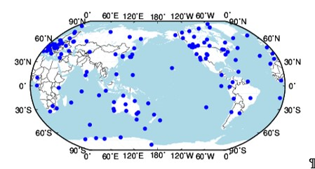
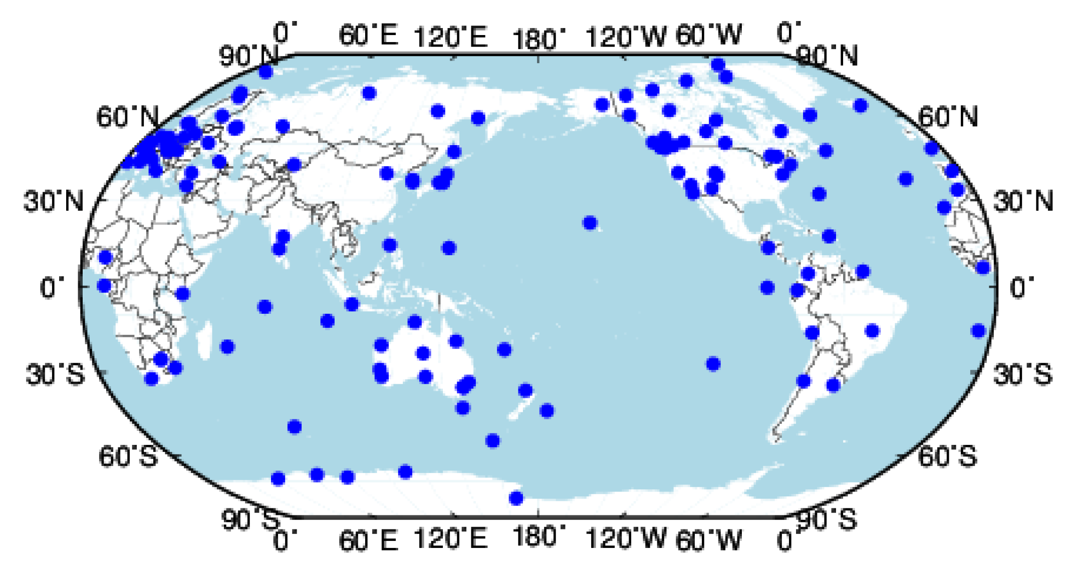
To validate the GLONASS pseudo-range ICB schemes for clock offset estimation, the observation data sampling 30 s of 110 IGS stations were selected, where the observation time covered six months, from 1 October 2018, to 31 March 2019. These stations are evenly globally distributed and equipped with receivers from seven manufacturers, as shown in
Table 1.
Figure 1 shows the geographic distribution of the selected stations.
There are two main steps in the clock offset estimation process. The first step is to obtain the ICBs based on SPP considering the ICB scheme in (8)–(11) separately. The approximate receiver and satellite clock offsets could also be obtained through this step. The second step is to combine the ICBs with Equations (6) and (7) to determine the final receiver and satellite clock offset.
Least-squares adjustment was used for the parameter estimation. To strengthen the functional model, the receiver coordinates were fixed according to the value in the IGS solution independent exchange (SINEX) product (
ftp://cddis.gsfc.nasa.gov/pub/gps/products/). The satellite positions were fixed and corrected by the Center for Orbit Determination in Europe (CODE) final orbit product (
ftp://cddis.gsfc.nasa.gov/pub/gps/products/). The first-order ionospheric delay was eliminated by the IF combination observations, and the high-order terms were omitted. The zenith troposphere delay was estimated as random walk noise (10
−7 m
2/s), the receiver clock offsets were estimated as white noise in each epoch, and the ambiguities were estimated as float constants for each arc. The satellite and receiver phase center offsets and variations were provided by igs14.atx. Furthermore, the phase windup and solid earth tide were considered. To reduce the pseudo-range noise and mitigate the multipath effect, the carrier-smoothed-code (CSC) approach was adopt to improve the accuracy of pseudo-range observation. The zenith-reference code and carrier phase standard deviation were empirically set as 0.3 m and 0.003 m, respectively, and observations set the elevation-dependent weight strategy. In addition, the elevation mask angle was set to 7° to track as many satellites as possible and to exclude particularly noisy and multipath effects.
3.1. GLONASS Pseudo-Range ICB Analysis
Based on the four ICB estimation strategies, we obtained the ICBs of GLONASS for each station from October 2018 to March 2019.
Figure 2 shows the R01 ICBs series for station receivers from seven different manufacturers. The three strategies (ICB-FPOL, ICB-RF, and ICB-RS) considering ICBs yielded similar values, ranging from −20 ns to 80 ns. The receiver at station ALBH was changed from a NET-G3A receiver to a SEPT POLARX5 receiver, which is why the ICBs exhibited a jump on 16 January 2019. For the same satellite, the ICBs corresponding to receivers from different manufacturers varied due to the dissimilar signal channels and manufacturers.
ICBs are site-individual, which may be influenced by site-specific factors such as the receiver and antenna types [
10,
12].
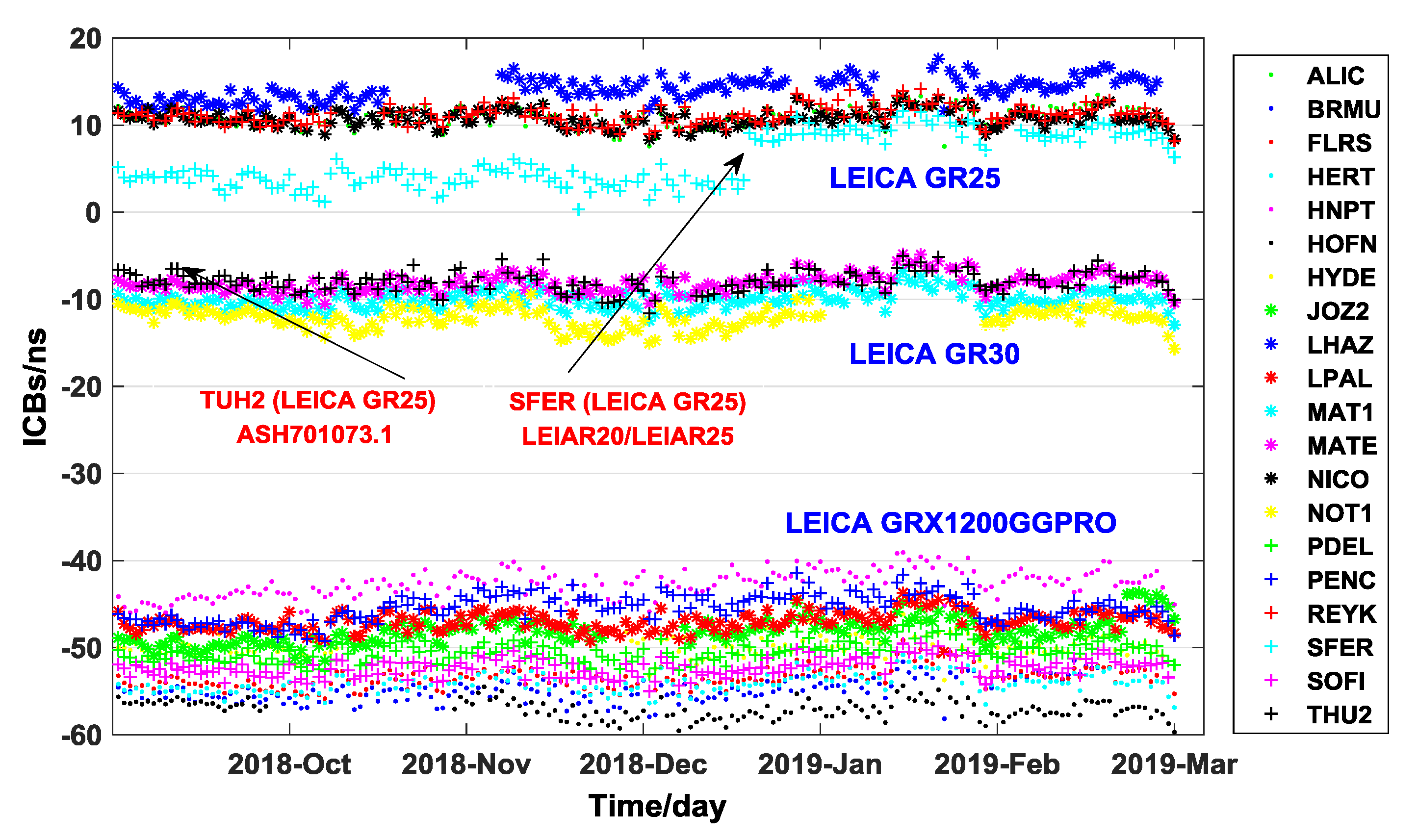
Figure 3 shows the R01 ICBs series for stations with three types of receivers from the same manufacturer, LEICA. These ICBs exhibited no significant jumps and remained quite stable over six months of daily processing. The ICBs obtained from the GR25, GR30, and GRX1200GGPRO receivers from the same manufacturer LEICA fell into three separate groups; however, the ICBs corresponding to the same receiver type agreed well over a certain value range. The ICBs of the LEICA GR25 and LEICA GR30 receivers were about 10 ns and −10 ns, respectively, while those of the GRX 1200 GGPRO receivers ranged from −50 ns to −60 ns. The ICB jump for the SFER station was attributable to an update of the receiver antenna from a LEIAR20 antenna to a LEIAR25 antenna on 17 January 2019. The ICBs of the TUH2 station differed from those of the other stations with LEICA GR25 receivers because this station was equipped with an ASH701073.1 antenna rather than a LEIAR antenna. As shown in
Table 2, certain stations have updated firmware, which had no effect on the ICBs. Additionally,
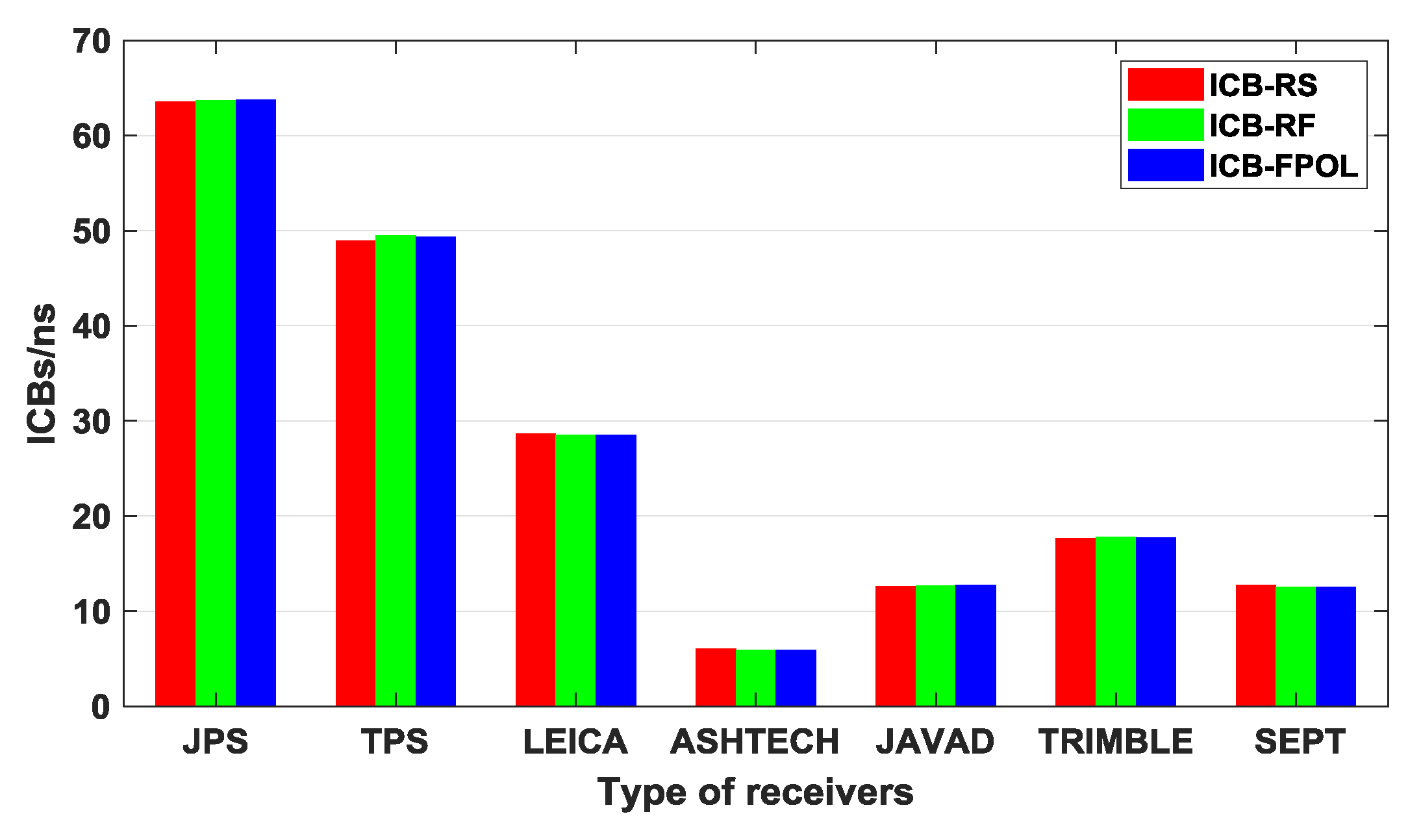
Figure 4 presents analyses of the average ICBs for each receiver type. The statistical results show that the ICB of the ASHTECH receiver was the lowest at approximately 5 ns and that of the JPS receiver was the highest at approximately 65 ns.
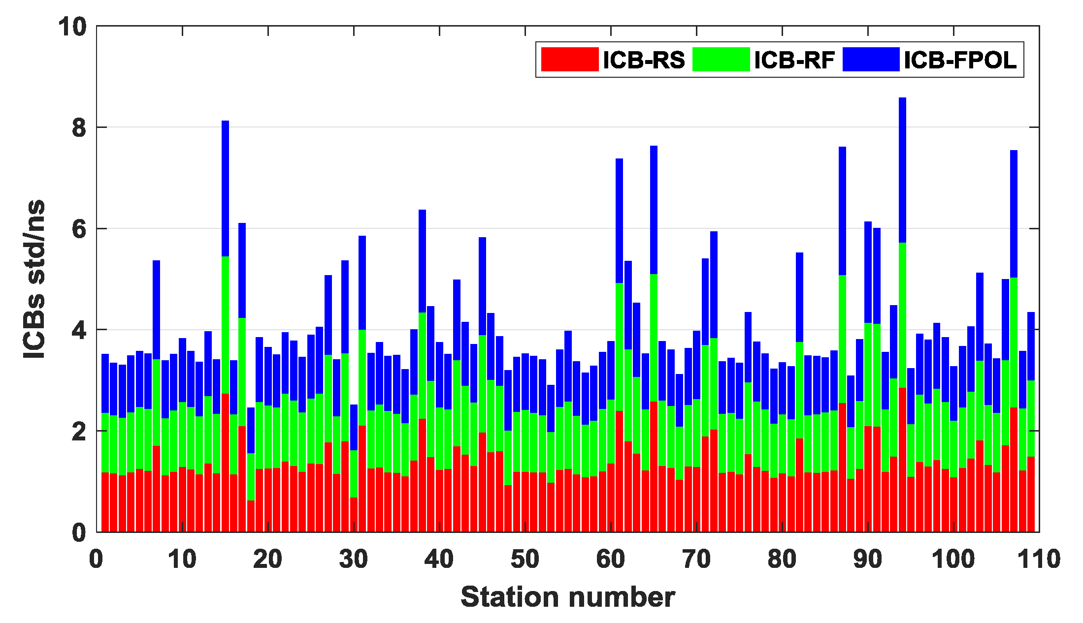
In addition,
Figure 5 presents the standard deviation (STD) of the ICB sequences obtained by the three ICB schemes (ICB-FPOL, ICB-RF, and ICB-RS) to demonstrate their stability. In general, the STD resulting from the three strategies agreed well, and the corresponding ICBs for each station were approximately 1 ns. The ICBs of some of the TRE_G3TH DELTA and POLARX5 receivers showed relative instability with a high STD of approximately 2 ns (the sum of the STDs was more than 4 ns). This result may be caused by the gross errors in the GLONASS pseudo-range observations of these stations. Overall, the stability of ICB-RS, which is independent of the GLONASS frequency, was optimal, with the lowest STD. The analysis results indicated that the ICBs on each day were stable, and the ICBs were related to the manufacturer, receiver, and antenna; however, the ICBs had no obvious relationship with the firmware version.
Regarding the ICB-RS model, we analyzed the ICBs of each satellite, and the results are shown in
Figure 6 and
Figure 7. The figures demonstrate that the ICBs of different satellites ranged from 60 ns to approximately 70 ns, with a discrepancy of approximately 10 ns (the absence of R06 and R12 was due to the lack of precise orbit information about these two satellites from CODE). The biases for the ICBs with the same frequency indices are shown in the lower part of
Figure 7 and ranged from 0.4 ns to 4 ns; these results indicated that the ICB was not strictly frequency dependent, but rather satellite specific. The differences may be due to the satellite space environment and discrepancies in the stability of atomic clock performance.
3.2. Estimated GLONASS Satellite Clock Offset Analysis
By combining the clock offset estimation strategy (6) with the ICBs corresponding to (8)–(11) individually, we obtained four kinds of estimated clock offsets. The six-month estimated satellite clock offsets resulting from the four constrained ICB strategies are then were evaluated by the European Space Operation Center (ESA), German Research Center for Geosciences (GFZ), and Information Analytical Center (IAC) final clock offset products. To evaluate the clock offset accuracy, the influence of the datum clock should be removed [
30,
31]. In addition, the difference in the orbital radial direction error, which is almost absorbed by the clock offset, should be considered [
30,
32].
Table 3 summarizes the average statistical accuracy of GLONASS according to three analysis center (AC) products. The three AC reference products yielded the same results, wherein the three models considering ICBs had accuracy superior to that of the ICB-NONE model. The ICB-NONE model, which ignores the ICBs, had the worst accuracy, with an STD of approximately 300 ps. This low accuracy was due to the ICB parameters being set to noise in the ICB-NONE scheme, causing the strict residual error checking process to remove many observations. However, the other three models, ICB-RS, ICB-RF, and ICB-FPOL, had the same level of accuracy of approximately 100 ps. The ICB-RS model had the smallest STD, which was superior to those of the ICB-RF and ICB-FPOL schemes.
3.3. Effects of ICBs on GLONASS PPP
As depicted in
Figure 4, the GLONASS pseudo-range ICBs can reach tens of nanoseconds. Thus, ICBs should be considered for PPP to obtain highly precise positioning results. PPP validation was performed before and after the pseudo-range ICB calibration by using the four kinds of estimated clock products, and the other products were fixed. We chose 20 IGS tracking stations distributed in middle and high latitude areas where there were more visible satellites [
33]. The GLONASS static and kinematic PPP were validated from 1 February 2019 to 14 February 2019, and the mean results are given in the following tables and figures.
Figure 8 displays the position error series of GLONASS static PPP of station HUEG with different ICB schemes. As for the static PPP, it took 47.5 min, 39 min, 24.5 min, and 20.5 min for ICB-NONE, ICB-FPOL, ICB-RF, ICB-RS, respectively, to converge to 0.1 m. The convergence performance of ICB-NONE was worse than the other three schemes owing to the neglect of the pseudo-range ICB.
Figure 9 shows the mean statistical accuracy of the GLONASS static PPP before and after ICB calibration at the 20 individual stations. Compared with the ICB-NONE model, which ignored the pseudo-range ICB, the positioning accuracy of the other three models was improved significantly. As shown by the mean statistical accuracy in
Table 4, the PPP with ICB calibration was improved to the level of millimeters in the north components. The mean 3D accuracy for the GLONASS static PPP was improved from 2.33 cm to 1.40 cm, 1.36 cm, and 1.31 cm, i.e., by 39.91%, 41.63%, and 43.78%, respectively. After considering pseudo-range ICB, the convergence performance was improved compared to ICB-NONE. Compared to ICB-NONE, the converging time of GLONASS static PPP improved from 37.44 min to 23.10 min, 20.16 min, and 16.24 min, i.e., by 38.3%, 44.95%, and 56.62%, respectively, after ICB calibration. The position performance of the scheme ICB-RS performed best among the four handling schemes because of the reasonable ICB estimation strategy and more accurate satellite clock offset product.
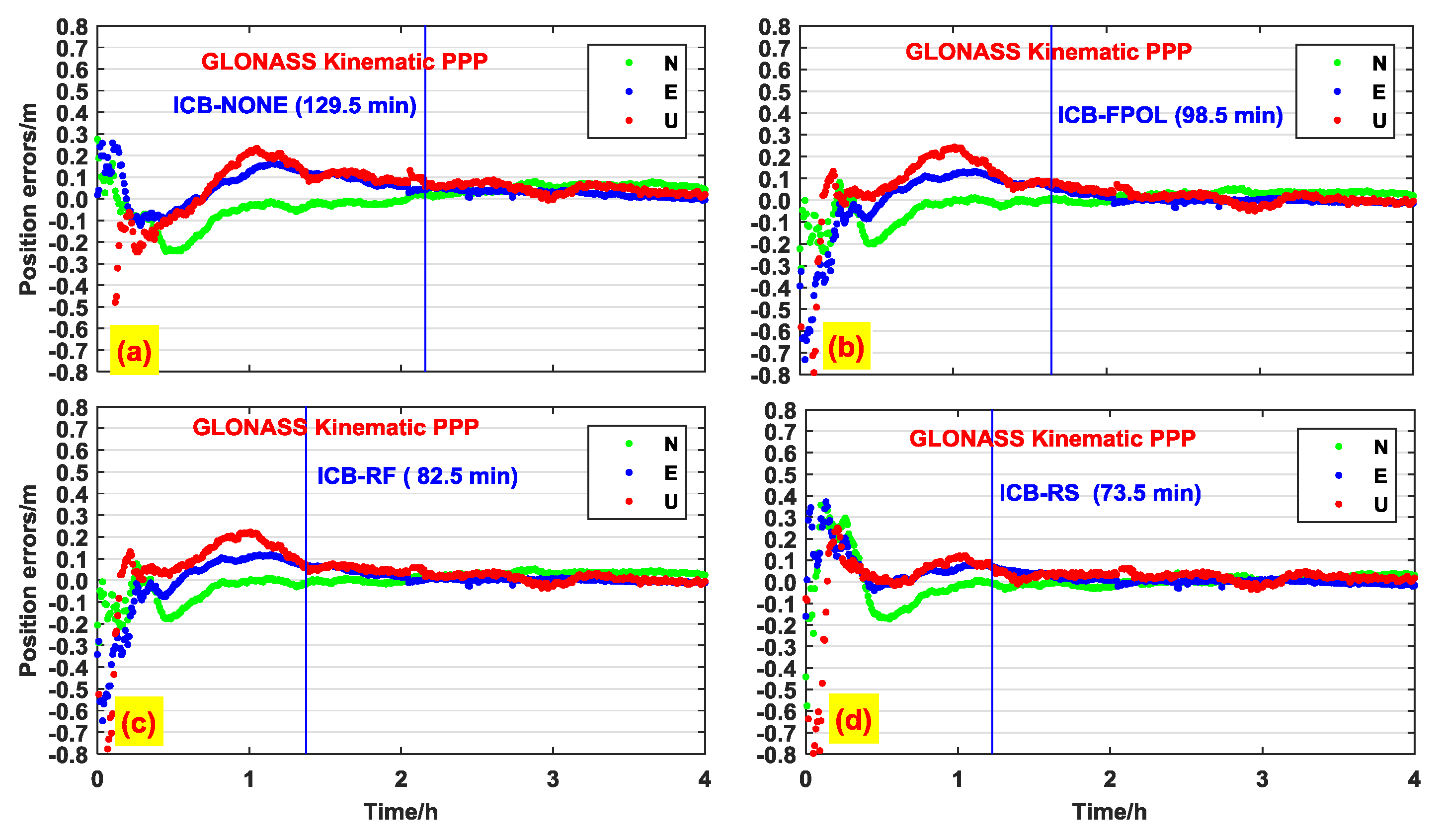
Furthermore,
Figure 10 displays the position error series of GLONASS kinematic PPP of station HUEG with different ICB schemes; the converging times were 129.5 min, 98.5 min, 82.5 min, and 73.5 min, respectively.
Figure 11 compares the solutions for GLONASS kinematic PPP before and after pseudo-range ICB calibration. The kinematic position precision was in the order of decimeters, which was worse than that of the static PPP.
As shown in
Table 4, the mean 3D accuracy of GLONASS kinematic PPP improved from 12.58 cm to 5.78 cm, 5.16 cm, and 4.53 cm, i.e., by 54.05%, 58.98%, and 63.99%, respectively, after ICB calibration. Regarding the kinematic GLONASS PPP, the improvement ratio of the up component was more remarkable, since the middle and high latitude areas have more visible GLONASS satellites and smaller geometric dilution of precision (GDOP) [
11,
17]. Additionally, for the converging time, it was improved from 96.41 min to 73.5 min, 67.98 min, and 65.26 min, i.e., by 23.763%, 29.49%, and 32.21%, respectively. Both the GLONASS PPP tests showed that the ICB-RS scheme was optimal, which was followed by the ICB-RF and ICB-FPOL schemes.
4. Pseudo-Range ICBs for GPS Test
Regarding GPS, the observations, particularly the code, were also affected by pseudo-range ICB dependent on receiver and satellite. This individual pseudo-range ICB was due to the different chip shape distortions among the GNSS satellites. Moreover, for different receivers with dissimilar correlator space, which provide different channels, the tracking biases may vary for each satellite [
18,
34]. These ICBs should be considered to be split into receiver and satellite-dependent parts in numerous applications, such as positioning with mixed signals and satellite clock offset estimation.
Considering the correlator space for different receivers or channels, we introduce an ICB parameter for each GPS pseudo-range observation equation, changing (4) into (12), which has the same form as for GLONASS:
here, a constraint is added for each GPS satellite, setting the sum of a specific satellite bias with respect to all the stations in the network to zero, where m is the number of receivers and S is the GPS satellite number, which ranges from 1 to 32:
4.1. Analysis of GPS Pseudo-Range ICBs
Similar to the GLONASS ICBs, the GPS pseudo-range ICBs were estimated based on different types of receivers, and the ICB characteristics were analyzed, as described in this section.
Figure 12 and
Figure 13 present the mean GPS pseudo-range ICBs for TRIMBLE and LEICA receivers from October 2018 to March 2019. The biases of the TRIMBLE and LEICA receivers were significant. The top plots in
Figure 12 and
Figure 13 show that the bias of each satellite had an extensive difference; the maximum bias was approximately 2.0 ns, and many satellites had bias around 1.0 ns. These ICBs were caused by individual chip shape distortions in the ranging signal, which led to different shifts of the correlator’s tracking channel for each pseudo random noise (PRN) and, consequently, different pseudo-range ICBs for each satellite [
34]. The bias of each satellite was stable from day to day with an STD around 0.1 ns, except for that of Block IIA satellite G04, which had poor stability than other on-board clocks.
4.2. Effects of GPS Pseudo-Range ICBs on Satellite Clock Offset Estimation
These pseudo-range ICB inconsistencies become apparent when products are derived based on data from a reference network with different types of receivers, which poses a challenge, for example, when clock offsets are estimated based on a network with mixed receiver types [
35]. The derived products then contain the average effect of the different ICBs. When a reference network consists of only one type of receiver with the same correlators, the products can be derived in a consistent manner [
13]. However, users with other incompatible receivers will experience inconsistencies in the clock offset and bias data from this network in their processing [
34].
Considering the effects of pseudo-range ICBs on clock offset estimation, we processed the GPS observations in the same manner as in the above GLONASS test from January 2019 to March 2019.
Figure 14 presents the accuracy series with respect to the IGS final clock offset product before and after ICB calibration. Most of the RMS lay within the range of 0.1 to 0.2 ns, and the scheme considering ICB had a mean RMS of 0.118 ns, which was better than the result of 0.163 ns when bias was neglected. The STD statistics over 90 days improved nearly 10 ps from 40 ps and 30 ps after ICB calibration. In summary, the effects of pseudo-range ICBs were noticeable in satellite clock offset estimation.
4.3. Effects of GPS Pseudo-Range ICBs on PPP
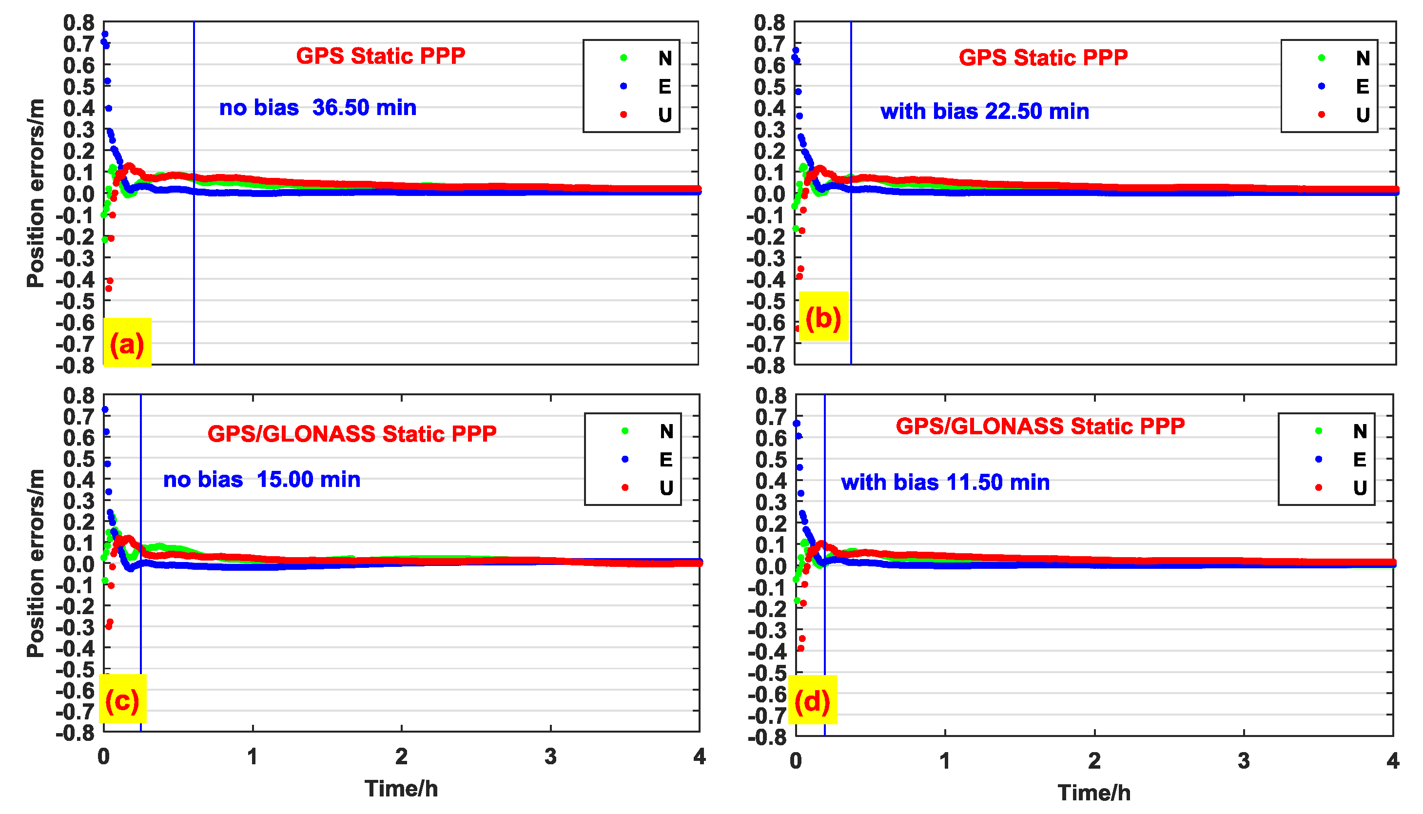
The pseudo-range ICBs in the code observations not only affect the code measurement accuracy, but also the quality of the PPP solutions. To evaluate the effects of the GPS pseudo-range ICBs, we validated the GPS and GPS/GLONASS PPP using the estimated clock offset.
Figure 15 display the position error series of GPS and GPS/GLONASS static PPP of station WTZR with different ICB schemes. We can see that it took 36.5 min and 15 min to converge to 0.1 m for GPS static PPP before and after pseudo-range ICB calibration, respectively, and for GPS/GLONASS, it was from 22.5 min to 11.5 min.
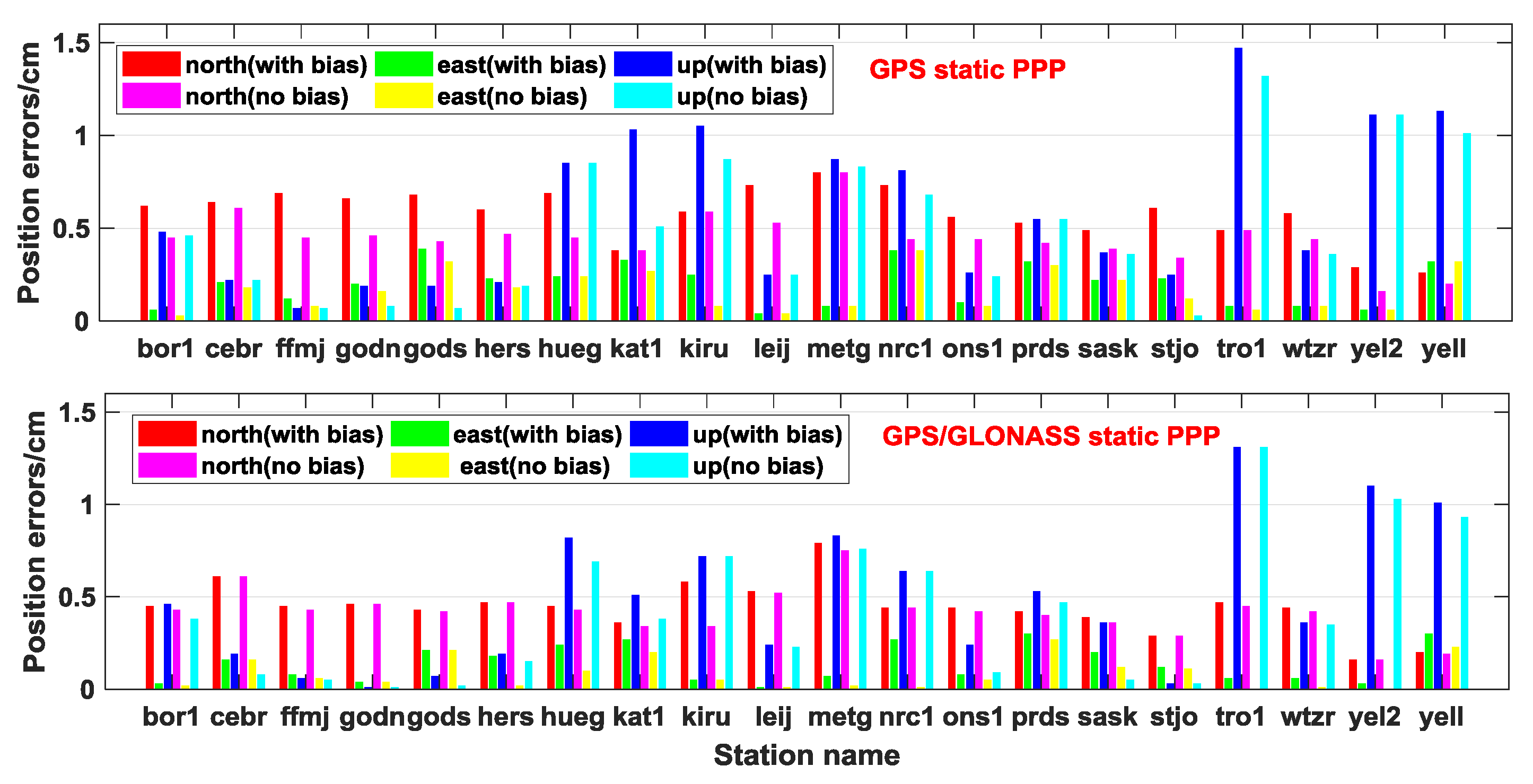
Figure 16 shows that the static PPP position accuracy improved after pseudo-range ICB calibration, and most of the position accuracies were in the order of millimeters. The
Table 5 show that the GPS PPP accuracy improved from 0.50, 0.28, and 0.81 cm to 0.37, 0.22, and 0.79 cm in the north, east, and up components, respectively, and the 3D orientation improved by 9.1%. Moreover, the combined GPS/GLONASS static PPP results improved from 0.35, 0.19, and 0.60 cm to 0.33, 0.12, and 0.55 cm in the north, east, and up components, respectively, and the 3D orientation improved by 9.72%. Additionally, the statistical results showed that the converging time of the GPS and GPS/GLONASS static PPP improved from 32.41 min and 17.56 min, to 20.3 min and 15 min, i.e., by 37.3% and 14.58%, respectively.
Furthermore, we compared the results for the kinematic PPP.
Figure 17 reveals the position error series of GPS and GPS/GLONASS kinematic PPP of station WTZR with different ICB schemes. For GPS kinematic PPP, the covering time was from 64 min to 48 min before and after pseudo-range ICB calibration; and for GPS/GLONASS, it was from 58.5 min to 12 min. As shown in
Figure 18, the position accuracy was on the order of centimeters.
Table 5 shows that the mean kinematic results of GPS improved from 1.34, 1.52, and 3.62 cm to 1.20, 1.22, and 3.25 cm, and the 3D orientation improved by 11.57%. Additionally, in the combined GPS/GLONASS kinematic PPP, the mean results improved from 1.09, 1.08, and 2.76 cm to 0.93, 0.87, and 2.33 cm, and the 3D orientation improved by 15.82%. As for the converging time, it improved from 60.78 min and 35.99 min to 40.66 min and 30.62 min, i.e., by 33.1% and 14.92%. Both tests indicated that the position accuracy could be significantly improved by GPS pseudo-range ICB calibration.
5. Conclusions
In this study, we adopted four strategies to estimate GLONASS pseudo-range ICBs by utilizing 110 globally evenly distributed IGS stations. In addition, the estimated ICBs were introduced into GLONASS satellite clock offset estimation using the corresponding strategies. We obtained significant results regarding ICB based on seven different manufacturer receivers. The three ICBs strategies (ICB-FPOL, ICB-RF, and ICB-RS) yielded similar values ranging from −20 to 80 ns. The ICBs corresponding to different types of receivers disagreed, due to different signal channels and manufacturer receiver types. In addition, we found that the type of antenna affected the ICBs, but the firmware version was irrelevant. The ICBs of GLONASS were stable over time, and the most stable strategy, ICB-RS, which was independent of the GLONASS frequency, exhibited the lowest STD. Furthermore, the ICBs had a non-negligible effect on the clock offset estimation. For GLONASS, the satellite clock offset accuracy was greatly improved from approximately 300 ps to 100 ps after ICB calibration, due to the ICB parameters being set to noise in ICB-NONE and, consequently, the strict residual error checking process in the clock offset estimation removed many observations. Regarding the PPP tests, pseudo-range ICB calibration accelerated the converging time by 40% and 30% for GLONASS static and kinematic PPP, respectively, and improved the mean RMS of the GLONASS static and kinematic PPP by approximately 40% and 50%, respectively. The up component improvement was more remarkable, which was related to the GLONASS having more visible satellites and smaller GDOP in middle and high latitude areas.
Furthermore, considering the different correlator channel designs of the receiver and different chip shape distortions among satellites, we attempted to introduce an ICB parameter into the GPS observation equation. According to the tests, the GPS pseudo-range ICB ranged from −2 ns to 2 ns. The influence of ICBs was noticeable in the satellite clock offset estimation, which could improve the GPS satellite clock offset accuracy by almost 10 ps. Based on the estimated clock offset and bias calibration for PPP, the GPS and combined GPS/GLONASS PPP could be improved by almost 10%. As for the converging time, it could accelerate the speed by 30% and 15% for GPS and GPS/GLONASS, respectively.
In general, the ICB scheme ICB-RS, which considers the ICB parameters for each GLONASS satellite, is the optimal choice in both the PPP and clock offset estimation. These results indicate that the GLONASS pseudo-range ICBs did not strictly obey frequency-specific or quadratic function relationships with the frequency number. For GPS, pseudo-range ICBs can also effectively improve the PPP and satellite clock offset estimation accuracy and accelerate the convergence in both static and kinematic PPP. Therefore, this work provides useful and meaningful insights into clock offset estimation and PPP applications. Subsequent analogical work will address the clock offset estimation of the globally developing Galileo and BDS.
Author Contributions
Q.A, B.Z., and T.X. conceived and designed the experiments; Q.A. performed the experiments, analyzed the data, and wrote the paper; B.Z., T.X., Y.Y. and Y.C. helped in the discussion and revision. All authors have read and agreed to the published version of the manuscript.
Funding
This work was supported by the National Key Research Program of China “Collaborative Precision Positioning Project” (No. 2016YFB0501900) funded by the Ministry of Science and Technology of the People’s Republic of China and the China Natural Science Funds (NSFC) (Nos. 41774042, 41804037, and 41231014). The third author is supported by the Chinese Academy of Sciences (CAS) Pioneer Hundred Talents Program. The second author acknowledges the Lu Jiaxi International Team program supported by the K.C. Wong Education Foundation and CAS.
Acknowledgments
The authors would like to acknowledge the IGS, MGEX for providing the observation data and precise products.
Conflicts of Interest
The authors declare no conflict of interest.
References
- Ge, M.; Gendt, G.; Rothacher, M.A.; Shi, C.; Liu, J. Resolution of GPS carrier-phase ambiguities in precise point positioning (PPP) with daily observations. J. Geod. 2008, 82, 389–399. [Google Scholar] [CrossRef]
- Geng, J.; Meng, X.; Dodson, A.H.; Ge, M.; Teferle, F.N. Rapid re-convergences to ambiguity-fixed solutions in precise point positioning. J. Geod. 2010, 84, 705–714. [Google Scholar] [CrossRef]
- Laurichesse, D.; Mercier, F.; BERTHIAS, J.P.; Broca, P.; Cerri, L. Integer ambiguity resolution on undifferenced GPS phase measurements and its application to PPP and satellite precise orbit determination. Navigation 2009, 56, 135–149. [Google Scholar] [CrossRef]
- Al-Shaery, A.; Zhang, S.; Rizos, C. An enhanced calibration method of GLONASS inter-channel bias for GNSS RTK. GPS Solut. 2013, 17, 165–173. [Google Scholar] [CrossRef]
- Kozlov, D. Statistical characterization of hardware biases in GPS+ GLONASS receivers. In Proceedings of the ION GPS-2000, Salt Lake City, UT, USA, 19–22 September 2000; pp. 817–826. [Google Scholar]
- Rossbach, U. Treatment of integer ambiguities in DGPS/DGLONASS double difference carrier phase solution. In Proceedings of the ION GPS-1996, Kansas City, MO, USA, 22–25 September 1996; pp. 909–916. [Google Scholar]
- Wanninger, L.; Wallstab-Freitag, S. Combined processing of GPS, GLONASS, and SBAS code phase and carrier phase measurements. In Proceedings of the ION GNSS 2007, Fort Worth, TX, USA, 25–28 September 2007; pp. 866–875. [Google Scholar]
- Yamada, H.; Takasu, T.; Kubo, N.; Yasuda, A. Evaluation and calibration of receiver inter-channel biases for RTK-GPS/GLONASS. In Proceedings of the ION GNSS 2010, Portland, OR, USA, 21–24 September 2010; pp. 1580–1587. [Google Scholar]
- Zinoviev, A.E. Using GLONASS in combined GNSS receivers: Current status. In Proceedings of the ION GNSS-2005, Long Beach, CA, USA, 14–18 September 2005; pp. 1046–1057. [Google Scholar]
- Chen, J.; Xiao, P.; Zhang, Y.; Wu, B. GPS/GLONASS system bias estimation and application in GPS/GLONASS combined positioning. In Proceedings of the China Satellite Navigation Conference (CSNC) 2013, Wuhan, China, 15–17 May 2013; pp. 323–333. [Google Scholar]
- Chuang, S.; Wenting, Y.; Weiwei, S.; Yidong, L.; Rui, Z. GLONASS pseudorange inter-channel biases and their effects on combined GPS/GLONASS precise point positioning. GPS Solut. 2013, 17, 439–451. [Google Scholar] [CrossRef]
- Reussner, N.; Wanninger, L. GLONASS inter-frequency biases and their effects on RTK and PPP carrier-phase ambiguity resolution. In Proceedings of the ION GNSS, Portland, OR, USA, 19–23 September 2011; pp. 712–716. [Google Scholar]
- Hauschild, A.; Montenbruck, O. The Effect of Correlator and Front-End Design on GNSS Pseudorange Biases for Geodetic Receivers. Navig. J. Inst. Navig. 2016, 63, 443–453. [Google Scholar] [CrossRef]
- Hauschild, A.; Montenbruck, O. A study on the dependency of GNSS pseudorange biases on correlator spacing. GPS Solut. 2014, 20, 159–171. [Google Scholar] [CrossRef]
- Tsujii, T.; Harigae, M.; Inagaki, T.; Kanai, T. Flight tests of GPS/GLONASS precise positioning versus dual frequency KGPS profile. Earth Planets Space 2000, 52, 825–829. [Google Scholar] [CrossRef]
- Kong, S.; Peng, J.; Liu, W.; Wang, M.; Wang, F. GNSS System Time Offset Real-Time Monitoring with GLONASS ICBs Estimated. In Proceedings of the 2018 IEEE 3rd International Conference on Image, Vision and Computing (ICIVC), Chongqing, China, 27–29 June 2018; pp. 837–840. [Google Scholar]
- Zhou, F.; Dong, D.; Ge, M.; Li, P.; Wickert, J.; Schuh, H. Simultaneous estimation of GLONASS pseudorange inter-frequency biases in precise point positioning using undifferenced and uncombined observations. GPS Solut. 2018, 22, 19. [Google Scholar] [CrossRef]
- Montenbruck, O.; Steigenberger, P.; Prange, L.; Deng, Z.; Zhao, Q.; Perosanz, F.; Romero, I.; Noll, C.; Stürze, A.; Weber, G. The Multi-GNSS Experiment (MGEX) of the International GNSS Service (IGS)–achievements, prospects and challenges. Adv. Space Res. 2017, 59, 1671–1697. [Google Scholar] [CrossRef]
- Zhang, B.; Chen, Y.; Yuan, Y. PPP-RTK based on undifferenced and uncombined observations: Theoretical and practical aspects. J. Geod. 2019, 93, 1011–1024. [Google Scholar] [CrossRef]
- Zhang, B.; Ou, J.; Yuan, Y.; Li, Z. Extraction of line-of-sight ionospheric observables from GPS data using precise point positioning. Sci. China Earth Sci. 2012, 55, 1919–1928. [Google Scholar] [CrossRef]
- Li, X.; Zhang, X.; Ge, M. Regional reference network augmented precise point positioning for instantaneous ambiguity resolution. J. Geod. 2011, 85, 151–158. [Google Scholar] [CrossRef]
- Chen, Y.; Yuan, Y.; Zhang, B.; Liu, T.; Ding, W.; Ai, Q. A modified mix-differenced approach for estimating multi-GNSS real-time satellite clock offsets. GPS Solut. 2018, 22, 72. [Google Scholar] [CrossRef]
- Li, W.; Wang, G.; Mi, J.; Zhang, S. Calibration errors in determining slant Total Electron Content (TEC) from multi-GNSS data. Adv. Space Res. 2019, 63, 1670–1680. [Google Scholar] [CrossRef]
- Liu, T.; Yuan, Y.; Zhang, B.; Wang, N.; Tan, B.; Chen, Y. Multi-GNSS precise point positioning (MGPPP) using raw observations. J. Geod. 2017, 91, 253–268. [Google Scholar] [CrossRef]
- Schaer, S. Société helvétique des sciences naturelles; Commission géodésique. In Mapping and Predicting the Earth’s Ionosphere Using the Global Positioning System; Institut für Geodäsie und Photogrammetrie Eidg. Technische Hochschule Zürich Arb.: Zürich, Switzerland, 1999; Volume 59. [Google Scholar]
- Oliver Montenbruck, A.H. Code biases in multi-GNSS point positioning. In Proceedings of the ION GNSS-2013, Nashville, TN, USA, 16–20 September 2013; pp. 616–628. [Google Scholar]
- Dach, R.; Walser, P. Bernese GNSS Software; Version 5.2; University of Bern, Bern Open Publishing: Bern, Switzerland, 2015. [Google Scholar]
- Liu, T.; Zhang, B.; Yuan, Y.; Zha, J.; Zhao, C. An efficient undifferenced method for estimating multi-GNSS high-rate clock corrections with data streams in real time. J. Geod. 2019, 93, 1435–1456. [Google Scholar] [CrossRef]
- Song, W.; Yi, W.; Lou, Y.; Shi, C.; Yao, Y.; Liu, Y.; Mao, Y.; Xiang, Y. Impact of GLONASS pseudorange inter-channel biases on satellite clock corrections. GPS Solut. 2014, 18, 323–333. [Google Scholar] [CrossRef]
- Chen, Y.; Yuan, Y.; Ding, W.; Zhang, B.; Liu, T. GLONASS pseudorange inter-channel biases considerations when jointly estimating GPS and GLONASS clock offset. GPS Solut. 2017, 21, 1525–1533. [Google Scholar] [CrossRef]
- Ge, M.; Chen, J.; Douša, J.; Gendt, G.; Wickert, J. A computationally efficient approach for estimating high-rate satellite clock corrections in realtime. GPS Solut. 2012, 16, 9–17. [Google Scholar] [CrossRef]
- Kouba, J.; Springer, T. New IGS station and satellite clock combination. GPS Solut. 2001, 4, 31–36. [Google Scholar] [CrossRef]
- Zheng, Y.; Nie, G.; Fang, R.; Yin, Q.; Yi, W.; Liu, J. Investigation of GLONASS performance in differential positioning. Earth Sci. Inform. 2012, 5, 189–199. [Google Scholar] [CrossRef]
- Hauschild, A.; Steigenberger, P.; Montenbruck, O. Inter-Receiver GNSS Pseudorange Biases and Their Effect on Clock and DCB Estimation. In Proceedings of the 32nd International Technical Meeting of the Satellite Division of the Institute of Navigation, Miami, FL, USA, 16–20 September 2019; pp. 159–171. [Google Scholar]
- Johnston, G.; Riddell, A.; Hausler, G. The international GNSS service. In Springer Handbook of Global Navigation Satellite Systems; Springer: Berlin/Heidelberg, Germany, 2017; pp. 967–982. [Google Scholar]
Figure 1.
Geographical distribution of the selected international global navigation satellite system (GNSS) service tracking stations.
Figure 1.
Geographical distribution of the selected international global navigation satellite system (GNSS) service tracking stations.
Figure 2.
ICB series for satellite R01 from October 2018 to March 2019.
Figure 2.
ICB series for satellite R01 from October 2018 to March 2019.
Figure 3.
ICB series for LEICA receivers of R01 from October 2018 to March 2019.
Figure 3.
ICB series for LEICA receivers of R01 from October 2018 to March 2019.
Figure 4.
Average ICBs for seven kinds of receivers.
Figure 4.
Average ICBs for seven kinds of receivers.
Figure 5.
Standard deviation (STD) resulting from the three kinds of ICB estimation strategies.
Figure 5.
Standard deviation (STD) resulting from the three kinds of ICB estimation strategies.
Figure 6.
GLONASS ICBs at the GODZ station from October 2018 to March 2019.
Figure 6.
GLONASS ICBs at the GODZ station from October 2018 to March 2019.
Figure 7.
Average ICBs at the GODZ station.
Figure 7.
Average ICBs at the GODZ station.
Figure 8.
GLONASS static precise point positioning (PPP) performance of station HUEG with different ICB schemes: ICB-NONE 47.50 min (a), ICB-FPOL 39.00 min (b), ICB-RF 24.50 min (c) and ICB-RS 20.50 min (d). The blue line is the place of converging time.
Figure 8.
GLONASS static precise point positioning (PPP) performance of station HUEG with different ICB schemes: ICB-NONE 47.50 min (a), ICB-FPOL 39.00 min (b), ICB-RF 24.50 min (c) and ICB-RS 20.50 min (d). The blue line is the place of converging time.
Figure 9.
GLONASS static PPP result based on different ICB schemes and corresponding clock offset.
Figure 9.
GLONASS static PPP result based on different ICB schemes and corresponding clock offset.
Figure 10.
GLONASS kinematic PPP performance of station HUEG with different ICB schemes: ICB-NONE 129.5 min (a), ICB-FPOL 98.5 min (b), ICB-RF 82.5 min (c) and ICB-RS 73.5 min (d).
Figure 10.
GLONASS kinematic PPP performance of station HUEG with different ICB schemes: ICB-NONE 129.5 min (a), ICB-FPOL 98.5 min (b), ICB-RF 82.5 min (c) and ICB-RS 73.5 min (d).
Figure 11.
GLONASS kinematic PPP result based on different ICB schemes and corresponding clock offset.
Figure 11.
GLONASS kinematic PPP result based on different ICB schemes and corresponding clock offset.
Figure 12.
GPS pseudo-range ICBs of LEICA receiver (the bias for each day is shown in a different color in the top plot).
Figure 12.
GPS pseudo-range ICBs of LEICA receiver (the bias for each day is shown in a different color in the top plot).
Figure 13.
GPS pseudo-range ICBs of TRIMBLE receiver (the bias for each day is shown in a different color in the top plot).
Figure 13.
GPS pseudo-range ICBs of TRIMBLE receiver (the bias for each day is shown in a different color in the top plot).
Figure 14.
Estimated GPS satellite offset accuracy with respect to IGS final clock offset product (the red points with bias correspond to the ICB calibration scheme, and the blue points with no bias correspond to the scheme in which the ICBs are neglected).
Figure 14.
Estimated GPS satellite offset accuracy with respect to IGS final clock offset product (the red points with bias correspond to the ICB calibration scheme, and the blue points with no bias correspond to the scheme in which the ICBs are neglected).
Figure 15.
GPS and GPS/GLONASS static PPP performance of station WTZR with different ICB schemes: GPS Static PPP no bias 36.50 min (a), GPS Static PPP with bias 22.50 min (b), GPS/GLONASS Static PPP no bias 15.00 min (c) and GPS/GLONASS Static PPP with bias 11.50 min (d).
Figure 15.
GPS and GPS/GLONASS static PPP performance of station WTZR with different ICB schemes: GPS Static PPP no bias 36.50 min (a), GPS Static PPP with bias 22.50 min (b), GPS/GLONASS Static PPP no bias 15.00 min (c) and GPS/GLONASS Static PPP with bias 11.50 min (d).
Figure 16.
Static PPP statistics before and after pseudo-range ICBs calibration.
Figure 16.
Static PPP statistics before and after pseudo-range ICBs calibration.
Figure 17.
GPS and GPS/GLONASS kinematic PPP performance of station WTZR with different ICB schemes: GPS Kinematic PPP no bias 64.0 min (a), GPS Kinematic PPP with bias 58.5 min (b), GPS/GLONASS Kinematic PPP no bias 48.0 min (c) and GPS/GLONASS Kinematic PPP with bias 12.0 min (d).
Figure 17.
GPS and GPS/GLONASS kinematic PPP performance of station WTZR with different ICB schemes: GPS Kinematic PPP no bias 64.0 min (a), GPS Kinematic PPP with bias 58.5 min (b), GPS/GLONASS Kinematic PPP no bias 48.0 min (c) and GPS/GLONASS Kinematic PPP with bias 12.0 min (d).
Figure 18.
Kinematic PPP statistics before and after pseudo-range ICBs calibration.
Figure 18.
Kinematic PPP statistics before and after pseudo-range ICBs calibration.
Table 1.
Receiver information used to estimate the inter-channel bias (ICB) and satellite clock offset.
Table 1.
Receiver information used to estimate the inter-channel bias (ICB) and satellite clock offset.
| Manufacturer | Type of Receiver | Number of Stations |
|---|
| JPS | LEGACY | 4 |
| EGGDT | 2 |
| TPS | NET-G3A | 8 |
| NETG3 | 2 |
| LEICA | GR25 | 6 |
| GRX1200GGPRO | 10 |
| GR30 | 3 |
| GRX1200+GNSS | 1 |
| ASHTECH | UZ-12 | 11 |
| JAVAD | TRE_G3TH DELTA | 16 |
| TRE_3 DELTA | 4 |
| TRIMBLE | NETR5 | 5 |
| NETR9 | 16 |
| SEPT | POLARX5 | 13 |
| SEPT POLARX4 | 9 |
Table 2.
Information about the LEICA receiver type, antenna type, and firmware version.
Table 2.
Information about the LEICA receiver type, antenna type, and firmware version.
| Station | Receiver Type | Antenna Type | Firmware |
|---|
| ALIC | LEICA GR25 | LEIAR25 | 4.20/4.30 |
| LHAZ | LEIAR25 | 4.12 |
| NICO | LEIAR25 | 4.12 |
| REYK | LEIAR25 | 4.31 |
| SFER | LEIAR20/LEIAR25 | 4.11 |
| THU2 | ASH701073.1 | 4.30 |
| BRMU | LEICA GRX1200GGPRO | JAVRINGANT_DM | 8.71/9.20 |
| FLRS | LEIAT504GG | 9.20 |
| HERT | LEIAT504GG | 7.80 |
| HNPT | LEIAX1202GG | 8.20/9.20 |
| HYDE | LEIAT504GG | 8.51 |
| JOZ2 | LEIAT504GG | 8.71 |
| LPAL | LEIAT504GG | 8.71 |
| PDEL | LEIAT504GG | 9.20 |
| PENC | LEIAT504GG | 9.20 |
| SOFI | LEIAR25 | 8.71 |
| HOFN | LEICA GRX1200+GNSS | LEIAR25 | 8.51/9.20 |
| MAT1 | LEICA GR30 | LEIAR20 | 4.20 |
| MATE | LEIAR20 | 4.20 |
| NOT1 | LEIAR20 | 4.20 |
Table 3.
Average accuracy for GLONASS satellites from October 2018 to March 2019.
Table 3.
Average accuracy for GLONASS satellites from October 2018 to March 2019.
| Acs/Model | ESA | GFZ | IAC |
|---|
| RMS (ps) | STD (ps) | RMS (ps) | STD (ps) | RMS (ps) | STD (ps) |
|---|
| ICB-NONE | 3945 | 338 | 4783 | 352 | 1732 | 303 |
| ICB-FPOL | 3670 | 115 | 3828 | 133 | 1288 | 99 |
| ICB-RF | 3629 | 80 | 3808 | 99 | 1230 | 94 |
| ICB-RS | 3299 | 78 | 3716 | 93 | 1183 | 85 |
Table 4.
PPP results based on different ICB models and corresponding clock offset products.
Table 4.
PPP results based on different ICB models and corresponding clock offset products.
| Model | Static GLONASS (cm) | | Kinematic GLONASS (cm) |
|---|
| N | E | U | 3D | 3D Improved | Convergence (min) | Convergence Improved | | N | E | U | 3D | 3D Improved | Convergence (min) | Convergence Improved |
|---|
| ICB-NONE | 1.01 | 0.95 | 1.87 | 2.33 | | 37.44 | | | 3.65 | 4.66 | 11.10 | 12.58 | | 96.41 | |
| ICB-FPOL | 0.65 | 0.30 | 1.20 | 1.40 | 39.91% | 23.10 | 38.30% | | 1.67 | 2.47 | 4.95 | 5.78 | 54.05% | 73.50 | 23.76% |
| ICB-RF | 0.64 | 0.29 | 1.16 | 1.36 | 41.63% | 20.61 | 44.95% | | 1.63 | 1.83 | 4.54 | 5.16 | 58.98% | 67.98 | 29.49% |
| ICB-RS | 0.63 | 0.29 | 1.11 | 1.31 | 43.78% | 16.24 | 56.62% | | 1.49 | 1.52 | 4.00 | 4.53 | 63.99% | 65.26 | 32.31% |
Table 5.
PPP results before and after pseudo-range bias calibration.
Table 5.
PPP results before and after pseudo-range bias calibration.
| Model | Static GPS (cm) | | Kinematic GPS (cm) |
|---|
| N | E | U | 3D | 3D Improved | Convergence (min) | Convergence Improved | | N | E | U | 3D | 3D Improved | Convergence (min) | Convergence Improved |
|---|
| No bias | 0.51 | 0.28 | 0.81 | 0.99 | | 32.41 | | | 1.34 | 1.52 | 3.62 | 4.15 | | 60.78 | |
| With bias | 0.37 | 0.22 | 0.79 | 0.90 | 9.09% | 20.30 | 37.37% | | 1.20 | 1.22 | 3.25 | 3.67 | 11.57% | 40.66 | 33.10% |
| Model | Static GPS/GLONASS (cm) | | Kinematic GPS/GLONASS (cm) |
| N | E | U | 3D | 3D Improved | Convergence (min) | Convergence Improved | | N | E | U | 3D | 3D Improved | Convergence (min) | Convergence Improved |
| No bias | 0.35 | 0.19 | 0.60 | 0.72 | | 17.56 | | | 1.09 | 1.08 | 2.76 | 3.16 | | 35.99 | |
| With bias | 0.33 | 0.12 | 0.55 | 0.65 | 9.72% | 15.00 | 14.58% | | 0.93 | 0.87 | 2.33 | 2.66 | 15.82% | 30.62 | 14.92% |
© 2020 by the authors. Licensee MDPI, Basel, Switzerland. This article is an open access article distributed under the terms and conditions of the Creative Commons Attribution (CC BY) license (http://creativecommons.org/licenses/by/4.0/).


