Technical Note

Comparison of Satellite-Derived Sea Surface Temperature and Sea Surface Salinity Gradients Using the Saildrone California/Baja and North Atlantic Gulf Stream Deployments

by
Jorge Vazquez-Cuervo
1,*,†,‡,
Jose Gomez-Valdes
2,‡ and
Marouan Bouali
3,‡
1
Jet Propulsion Laboratory, California Institute of Technology, Pasadena, CA 91109, USA
2
Physical Oceanography Department, Center for Scientific Research and Higher Education at Ensenada, Ensenada 22860, Baja California, Mexico
3
Institute of Oceanography, University of São Paulo, São Paulo 05508-120, Brazil
*
Author to whom correspondence should be addressed.
Current address: 4800 Oak Grove Dr. M/S 300/323, Pasadena, CA 91109, USA.
These authors contributed equally to this work.
Remote Sens. 2020, 12(11), 1839; https://doi.org/10.3390/rs12111839
Submission received: 20 April 2020 / Revised: 29 May 2020 / Accepted: 1 June 2020 / Published: 6 June 2020

Abstract

:
Validation of satellite-based retrieval of ocean parameters like Sea Surface Temperature (SST) and Sea Surface Salinity (SSS) is commonly done via statistical comparison with in situ measurements. Because in situ observations derived from coastal/tropical moored buoys and Argo floats are only representatives of one specific geographical point, they cannot be used to measure spatial gradients of ocean parameters (i.e., two-dimensional vectors). In this study, we exploit the high temporal sampling of the unmanned surface vehicle (USV) Saildrone (i.e., one measurement per minute) and describe a methodology to compare the magnitude of SST and SSS gradients derived from satellite-based products with those captured by Saildrone. Using two Saildrone campaigns conducted in the California/Baja region in 2018 and in the North Atlantic Gulf Stream in 2019, we compare the magnitude of gradients derived from six different GHRSST Level 4 SST (MUR, OSTIA, CMC, K10, REMSS, and DMI) and two SSS (JPLSMAP, RSS40km) datasets. While results indicate strong consistency between Saildrone- and satellite-based observations of SST and SSS, this is not the case for derived gradients with correlations lower than 0.4 for SST and 0.1 for SSS products.

Graphical Abstract

1. Introduction

The paper aims to follow-up on the work of [1], where the authors compared sea surface temperatures (SSTs) and sea surface salinities (SSSs) from the Saildrone deployment along the California and Baja coasts with satellite-derived products. For SST, six GHRSST compliant Level 4 products were used for the comparison, namely the Multi-Scale Ultra-High Resolution (MUR) SST, the Operational Sea Surface Temperature and Sea Ice Analysis (OSTIA) SST, the Canadian Meteorological Center (CMC) SST, the NAVOCEANO K10 SST, the Remote Sensing Systems (RSS) REMMS_MW_IR SST and the Danish Meteorological Institute (DMI) SST. The primary conclusions of the paper showed good agreement (i.e., correlations higher than 0.95) between Saildrone and satellite-derived SSTs.
For SSS, the authors analyzed the Jet Propulsion Laboratory Captive Active Passive (CAP) SSS and the Remote Sensing Systems (RSS) 40- and 70 km-derived SSS products from the Soil Moisture Active Passive (SMAP) satellite. Salinity comparisons showed significantly lower signal-to-noise ratios than those on SST, an indication that land contamination and the lower spatial resolution were both contributing to the lower correlations in the SSS comparisons [2]. The Saildrone California/Baja campaign was also used in [3] for the validation of additional parameters that include satellite-derived sensible heat fluxes and wind vectors. On Saildrone, the SST and SSS Conductivity Temperature Depth Profilers (CTD), are only two of the multiple instruments onboard. Other sensors include a fluorometer, as well as an Acoustic Doppler Current Profiler (ADCP). For a complete description of the Saildrone instrumentation and known accuracies, see [3].
In this study, we extend the previous results by comparing satellite-based SST and SSS gradients with Saildrone measurements. The importance of also validating gradients with in situ measurements has been confirmed for both a data quality and scientific perspective [4,5]. References [6,7] have shown the coupling between the wind stress curl and SST gradients. Reference [6] found that the wind stress divergence was linearly related to the downwind SST gradients in the Eastern Tropical Pacific. The results clearly showed the air-sea coupling to be associated with the formation of thermal surface fronts. Reference [7] examined the coupling in the Cape Frio coastal upwelling region off Southeastern Brazil. They determined that wind stress curl was more strongly correlated with SST gradients than SST. Thus, SST gradients were critical for the relationship between wind stress curl and the formation of localized upwelling events. A significant conclusion of the work was how wind stress curl could be modified through feedback mechanisms associated with coastal upwelling. In [8] one also found strong summertime coupling between wind stress and the formation of SST fronts in the California Current associated with coastal upwelling. The summertime coupling is associated with the seasonal intensification of the coastal upwelling system. The coupling was determined to exist for both wind stress divergence and wind stress curl. The results point to the importance of SST gradients in air–sea coupling. As such, precise and accurate measurements of gradients become critical for numerical modeling, inclusive of numerical weather prediction. In [9] it was found that despite statistical consistency, there were differences in SST gradients based on the application of the multi-channel sea surface temperature (MCSST) algorithm or the non-linear (NLSST) sea surface temperature algorithm. They concluded that differences as large as 0.02 °C/km between SST gradient magnitudes derived from the two algorithms were most likely due to the use of the first-guess SST field in the NLSST formulation. Unlike the MCSST, the magnitude of SST gradients derived from NLSST showed a clear correlation with SST values. Other studies [10] have also shown that there are warm satellite SST biases in the Eastern Boundary Current regions. In a study comparing Terra MODIS SST and AVHRR SST Pathfinder with in situ data, the authors found warm summertime SST biases in four major upwelling regions, with values as high as 3 to 5 °C. Such biases are due to the over-flagging of valid SST pixels associated with anomalous cold events typical in upwelling regions. More recently, ref. [11] found large biases when comparing several Level 4 SST datasets with buoy measurements during coastal upwelling events. In [12], these biases were also observed in Level 2 MODIS data despite using an improved cloud-masking method [13] and can be attributed to the calibration of Level 2 SST retrieval algorithms [14,15] which is based on global in situ measurements and thus does not account for atmospheric processes specific to coastal upwelling regions. These biases may also be due to the fact that satellite-based SST is an estimate of the top layer of the ocean surface (∼1 micrometer), whereas the Saildrone sensor, being placed below the surface, measures cooler or warmer temperatures depending on the mixing processes involved in a given region or during a specific season.
Overall, warm SST biases, along with the air-sea coupling and an associated relationship to SST gradients, make the case that the validation of both SST and SSS, along with their respective gradients, is critical for coastal upwelling regions. In this work, we focus on two oceanic regions usually associated with spatial-temporal variability, i.e., a coastal upwelling region and a Western Boundary Current region. The unique ability of Saildrone to sample at high spatio-temporal resolutions over an extended period (i.e., several months) allows for the validation of both SST, SSS, and their corresponding gradients using data from two separate campaigns conducted in the California/Baja region and in the North Atlantic Gulf Stream.

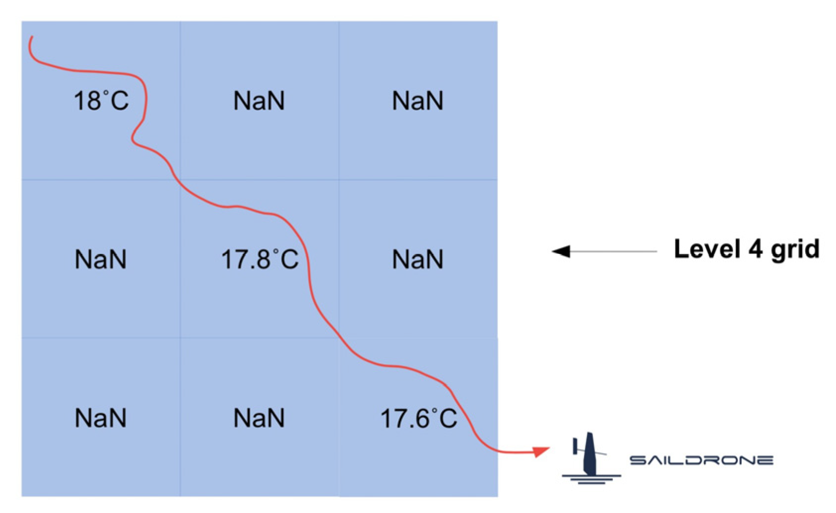
2. Methodology and Data

The validation of satellite SST/SSS gradients using standard in situ measurements derived from Argo floats and tropical/coastal moored buoys is a challenging task due to the very different nature of acquired signals. Gradients estimated from satellite observations are bi-dimensional vectors with a given magnitude and orientation, whereas in situ data are collected at one particular geographical location. The high temporal frequency of Saildrone measurements along its trajectory (1 per minute) allows one to see the acquired data as a one-dimensional signal where values vary as a function of time. Given that the sampling frequency of Saildrone is significantly higher than the temporal scale of ocean submesoscale processes, gradients in the spatial domain can be estimated from successive measurements. One possible approach to compare satellite-based gradients with those obtained from Saildrone is to rely on finite differences. In a lat/lon grid, for example, the magnitude of the SST gradient at the location (i, j) is typically estimated using a finite central differences scheme as follows
| SST ( i , j ) | = ( [ S S T ( i 1 , j ) S S T ( i + 1 , j ) d i 1 , j i + 1 , j ] 2 + [ S S T ( i , j 1 ) S S T ( i , j + 1 ) d i , j 1 i , j + 1 ] 2 ) 1 2
where d i 1 , j i + 1 , j represents the distance in kilometers between grid points (i − 1, j) and (i + 1, j). However, this commonly used approach significantly limits the number of grid points where satellite-based gradients can be compared with the Saildrone data. In fact, such a method requires the Satellite/Saildrone collocated observations to be available for all four locations (i − 1, j), (i + 1, j), (i, j − 1) and (i, j + 1), which is seldom the case. Figure 1 shows a typical configuration of Saildrone trajectory where SST gradients from Level 4 collocated data cannot be computed due to missing values in both vertical and horizontal directions. While using a forward or backward finite differences scheme may alleviate this issue (i.e., when the Saildrone trajectory allows two consecutive collocated values along vertical and horizontal directions), an alternative method is required for the validation of SST gradients.
In this paper, we adopt a different collocation strategy from that used for the validation of SST and SSS in [1]. In the following, we denote ds as the spatial resolution of the Level 4 satellite SST/SSS field. For each grid point (i, j), all Saildrone measurements acquired between latitudes ids and i + ds and longitudes jds and j + ds are averaged. This leads to a collocated dataset of Saildrone and satellite-based SST/SSS values in the lat/lon grid. For each location (i, j), we also compute the average time of all Saildrone measurements, which is then sorted to derive the collocated time series of SST (SSS), denoted hereafter as Sat_SST (Sat_SSS) and Sail_SST (Sail_SSS) for the satellite and Saildrone observations, respectively. The temporal window used for the collocation is the temporal resolution of the Level 4 datasets, i.e., one day. The magnitude of SST gradients can then be approximated using forward finite differences of successive measurements, i.e.,
| SST ( t ) | = | S S T ( t + 1 ) S S T ( t ) | d t t + 1
where d t t + 1 represents the distance between collocated observations obtained at times t + 1 and t. We use Equation (2) to calculate the magnitude of SST gradients from Saildrone and various Level 4 SST products. Grid points with less than 50 Saildrone measurements are discarded as the average of in situ SST may not be representative of the SST value inside the grid point. Note that experiments conducted with a higher number of Saildrone measurements for each grid point have little impact on the results reported in the next section. In this study, six GHRSST compliant Level 4 SST datasets have been used, namely
(1)
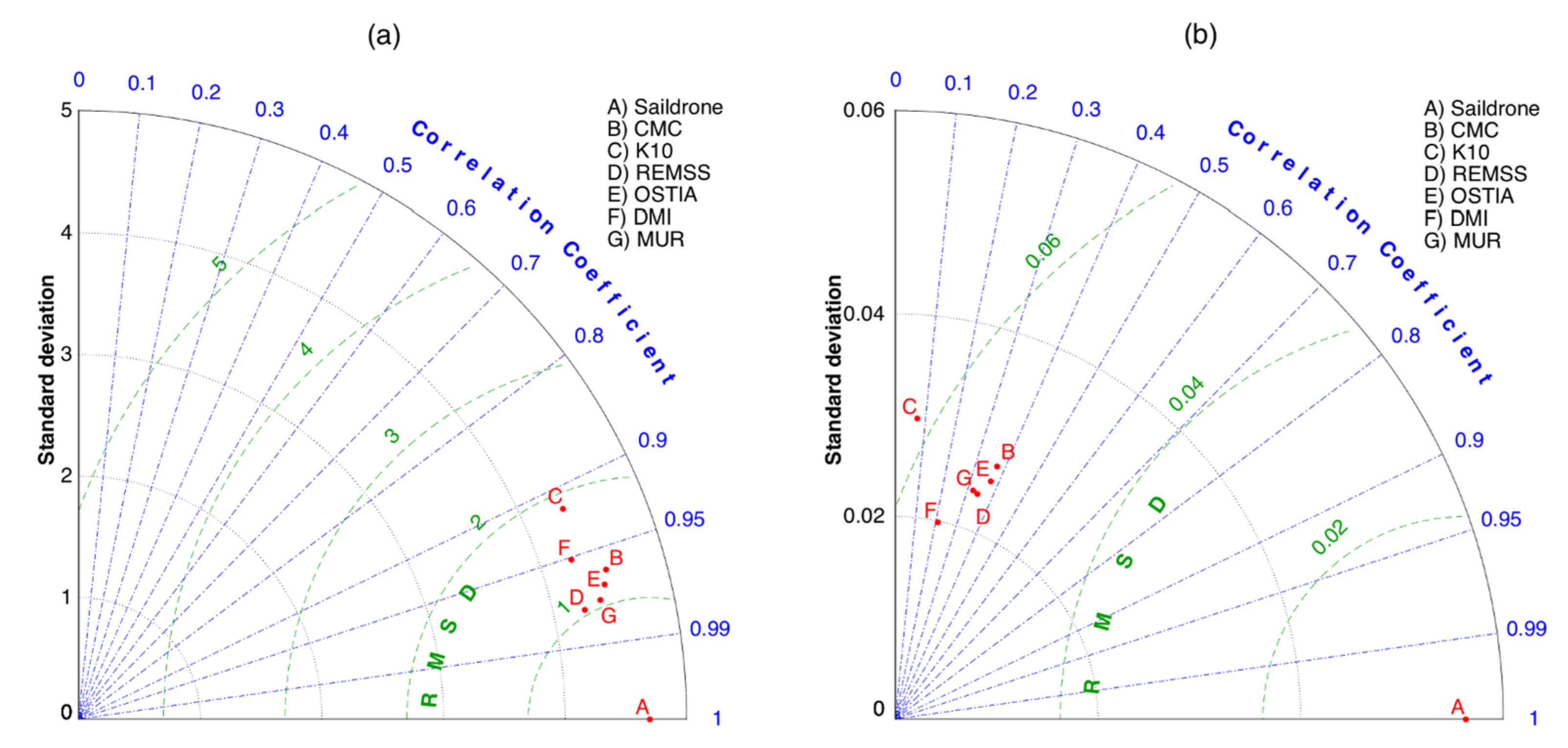
the Canadian Meteorological Office CMC;
(2)
the Naval Oceanographic Office NAVO K10;
(3)
the Remote Sensing Systems REMSS_MW_IR;
(4)
the UK Meteorological Office OSTIA;
(5)
the Danish Meteorological Institute DMI; and
(6)
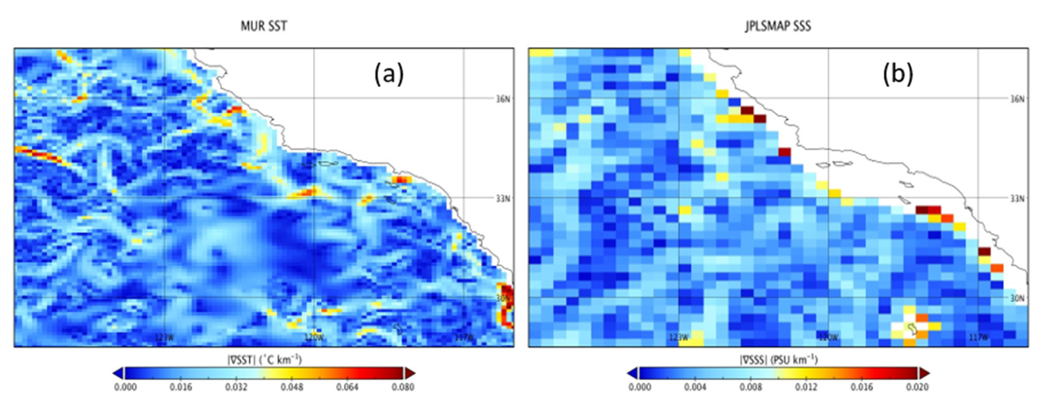
the Jet Propulsion Laboratory MUR.
In addition, two daily SSS datasets produced from 8-day running mean were selected:
(1)
the Jet propulsion Laboratory version 4.0 Soil Moisture Active Passive (SMAP) (JPLSMAP); and
(2)
the Remote Sensing Systems version 4.0, 40 km (RSS40) dataset.
A detailed description of these SST datasets can be found in [1]. Both SST and SSS datasets were downloaded from the Physical Oceanography Distributed Active Archive Center (PO.DAAC, https://podaac.jpl.nasa.gov/) and reprojected into a 0.1° and 0.25° resolution grid, respectively, using bilinear interpolation. Previous results [9] had already demonstrated how the high correlation between SST values derived from various satellite products does not necessarily apply when analyzing SST gradient magnitudes. In this paper, we used two different Saildrone campaigns for the validation of satellite SST/SSS gradients. The first 60-day campaign, which was used to validate of SST and SSS in [1], was conducted over the period from 11 April 2018 to 11 June 2018 in the California/Baja region (round cruise from San Francisco Bay down to Guadalupe Island). The California/Baja Saildrone campaign data can be download from the PO.DAAC. The second 27-day Saildrone campaign was conducted in the North Atlantic Gulf Stream region from 30 January 2019 to 25 February 2019, and the corresponding data can be downloaded from the European Marine Observation and Data Network (https://www.emodnet-physics.eu/Portal/).

3. Results

The California Current Upwelling System (CCUS) and the North Atlantic Gulf Stream (NAGS) have been selected in this study as they are representative of the large spatio-temporal variability associated with both mesoscale and submesoscale fronts. Using the methodology described in the previous section, we generated time series of SST/SSS gradient magnitude for the two Saildrone campaigns. Due to the high temporal variability of SST/SSS gradients, the time series are not shown here. Instead, NetCDF files containing latitude, longitude, time, SST/SSS values, and derived gradients are provided in the supplemental files.

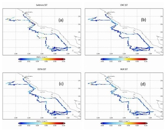
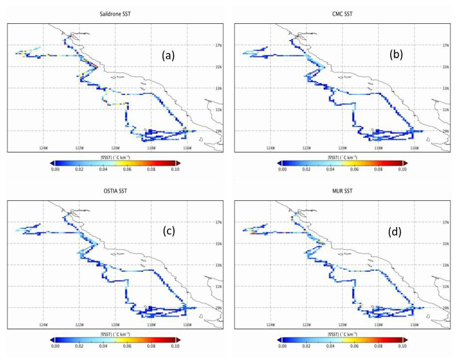
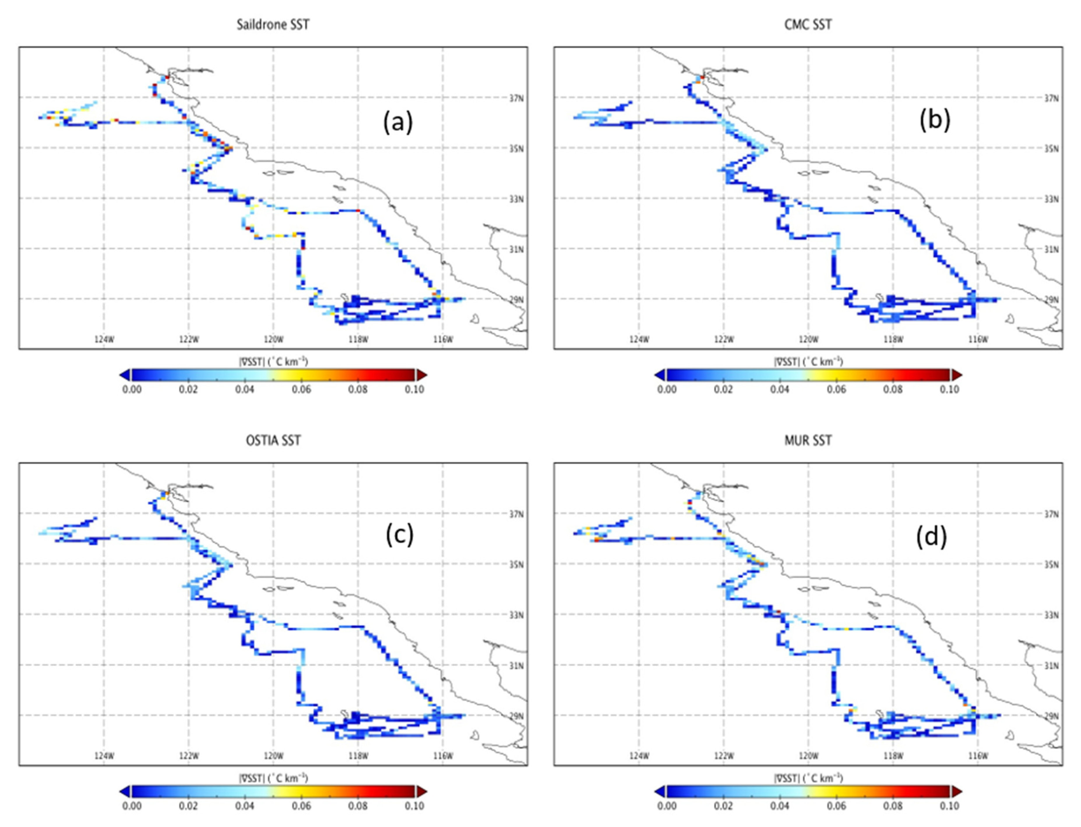
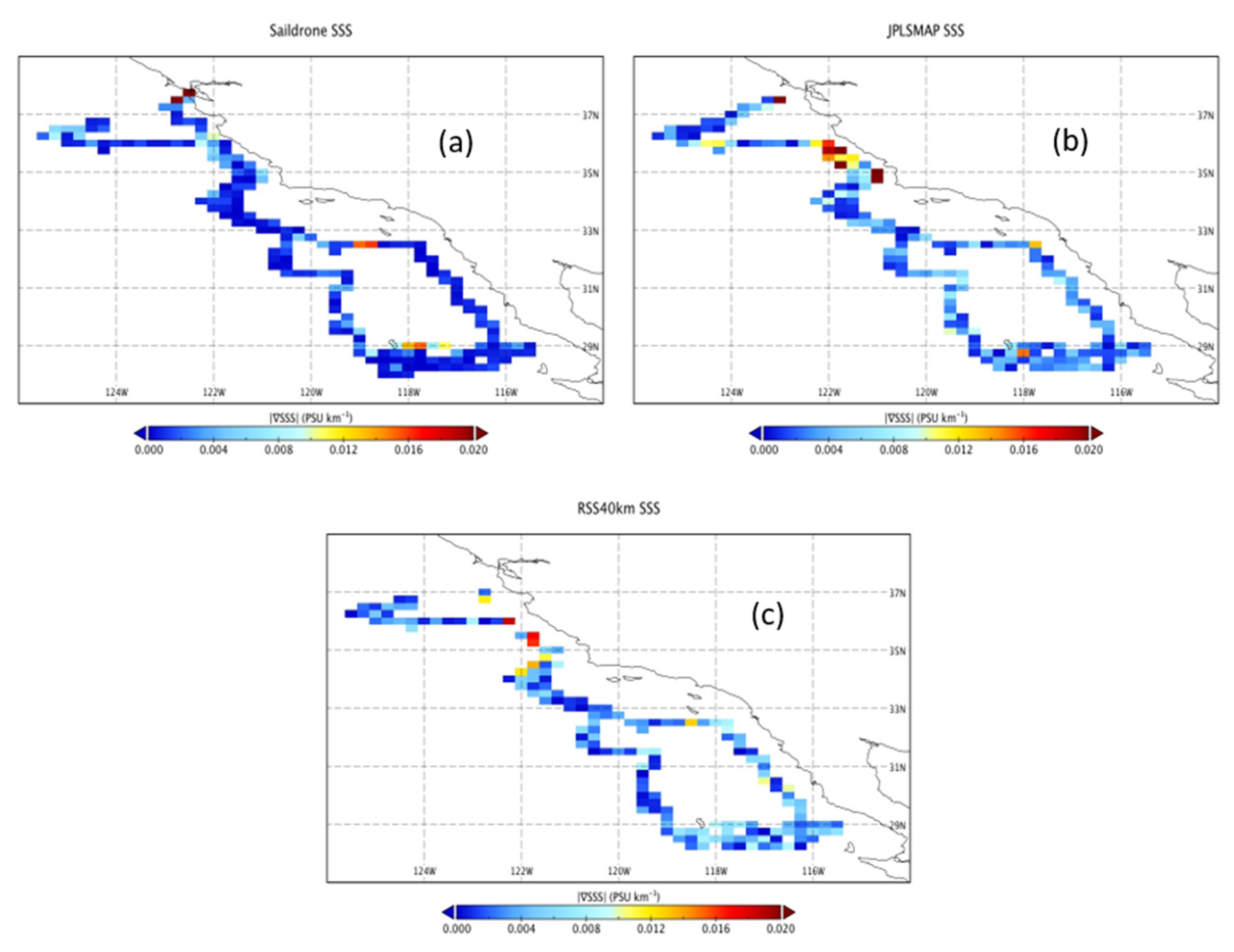
3.1. California Current Upwelling System (CCUS)

Figure 2 shows the magnitude of SST gradients derived from the Saildrone and collocated Level 4 CMC, OSTIA, and MUR along the Baja California deployment. First, we note that the Saildrone captures a more important number of high SST gradients compared to all Level 4 SST datasets. The magnitude of SST gradients captured by Saildrone in the CCUS can reach values above 0.1 °C/km, whereas for CMC, and OSTIA, maximum values are mostly lower than 0.04 °C/km. This can be explained by the use of optimal interpolation and the underlying spatio-temporal smoothing, which does not preserve small scale features. The Level 4 MUR, which is based on wavelet analysis, is able to capture higher magnitudes of SST gradients with maximum values of the order of 0.75 °C/km. As expected, while Saildrone and Satellite SST simultaneously observed several thermal fronts, the magnitude of gradients is significantly underestimated in Level 4 SST analysis, which only provides a daily estimate of the SST field as opposed to the synoptic observation from Saildrone. In contrast, the analysis of SSS gradients illustrated in Figure 3 indicates that higher gradients are found in satellite products compared to Saildrone. Significant differences of up to 0.02 PSU/km between the magnitude of SSS gradients in JPLSMAP/ RSS40km and Saildrone are observed. The maps of Figure 3 indicate that these discrepancies increase as the Saildrone gets closer to the coast. This can be seen in the Saildrone track portions located between 34 and 36° N and between 29 and 32° N and is likely due to land contamination as well as a larger spatial scale of passive microwave sensors, which affects the accuracy of satellite SSS values and, consequently, associated gradients.

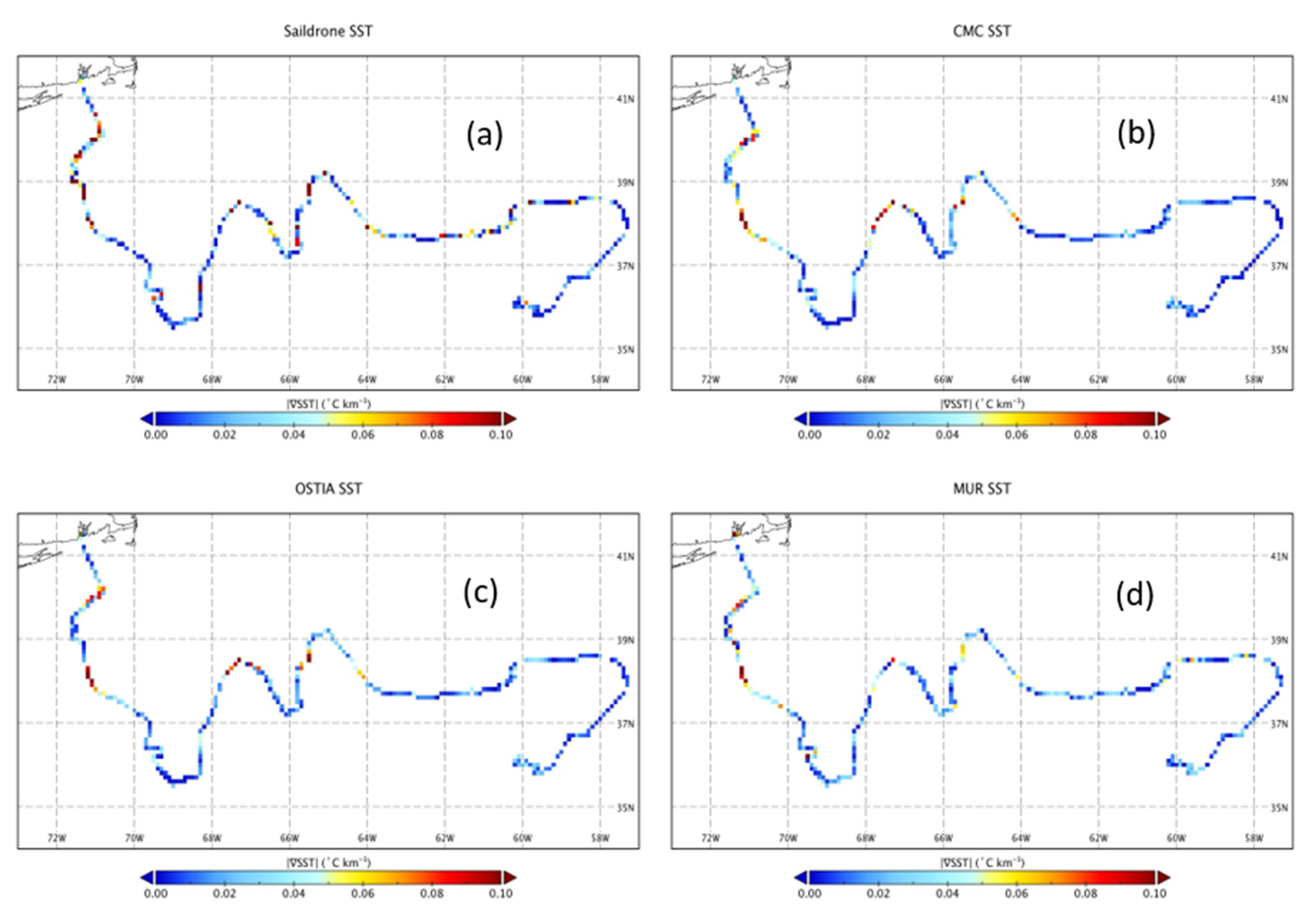
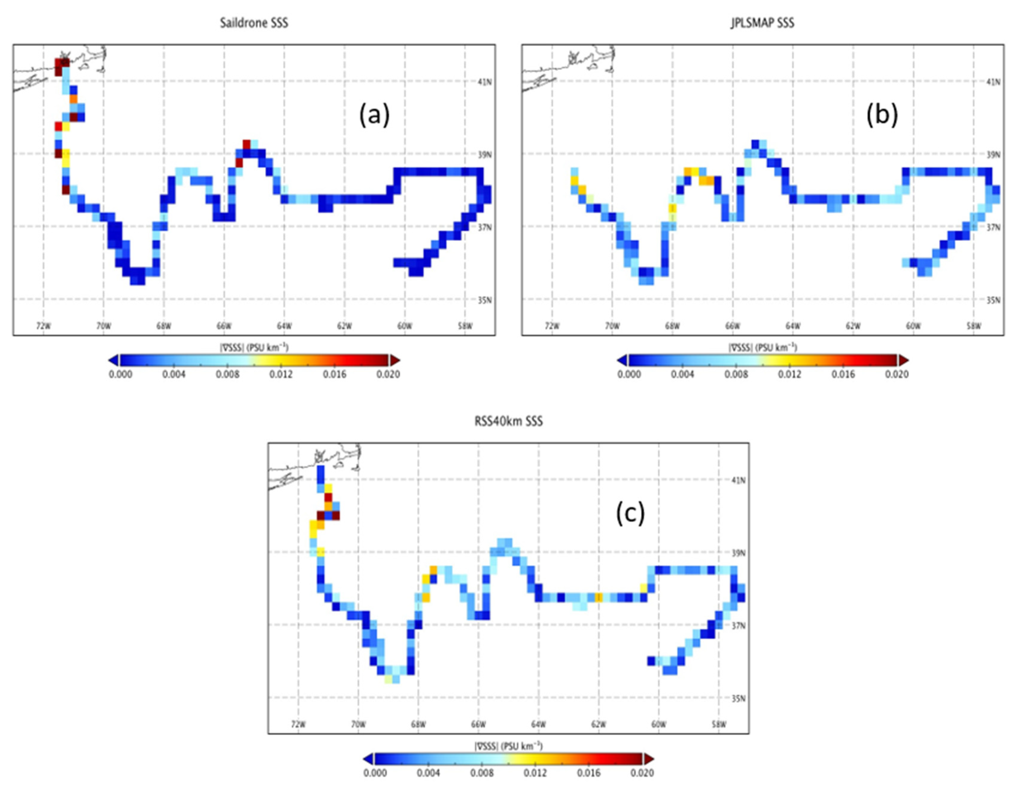
3.2. North Atlantic Gulf Stream (NAGS)

Figure 4 shows the values of SST gradient magnitudes for Saildrone, CMC, OSTIA, and MUR along the NAGS deployment. Similar to what is observed in the CCUS campaign, we note that gradients in Level 4 SST are also significantly underestimated in the NAGS region. Maximum SST gradients associated with frontal activity in the GS and measured by Saildrone exceed values of 0.2 °C/km. However, for CMC, OSTIA, and MUR, most thermal fronts have magnitudes lower than 0.1 °C/km. In this region dominated by intense mesoscale and submesoscale surface fronts, the average of SST gradient magnitudes for the entire campaign period for MUR, for example, is 0.22 °C/km, whereas Saildrone measured an average of 0.35 °C/km. Analysis of SSS gradients illustrated in Figure 5 also indicates significant discrepancies between Saildrone and satellite observations, including in areas distant from the coast. As an example, at the end of the campaign, i.e., in the area located between 35–38° N and 57–60° W, RSS40km and JPLSMAP measure many gradients with values higher than 0.005 PSU/km, whereas most values derived from Saildrone are lower than 0.001 PSU/km. Overall, maps of SST and SSS gradients in the CCUS and the NAGS show that the differences between Saildrone and satellite datasets are related not only to the magnitude but also to the location of temperature and salinity fronts.
To further analyze the consistency between Saildrone- and satellite-based observations, biases, root mean square differences, and correlation coefficients were computed. Values for both SST/SSS and derived gradients are reported in Table 1 for the CCUS and Table 2 for the NAGS regions. We note that for both campaigns, correlation coefficients with Saildrone are higher than 0.96 for all level 4 products. We also note that, overall, SST biases in the NAGS are slighter higher than those observed in the CCUS, where all biases are below 0.15 °C in absolute value, with the exception of MUR (bias of the order of 0.285°). The differences in SST validation statistics between the CCUS and the NAGS can be attributed to the amount of cloud coverage in these regions as well as the higher magnitude of thermal fronts in the NAGS, which can lead to over-masking of valid pixel values. Overall, results reported in Table 1 and Table 2 for SST indicate that all Level 4 datasets are statistically consistent with the Saildrone data. However, this is not the case when analyzing corresponding gradients. Correlation coefficients computed for the magnitude of SST gradients are lower than 0.4 for both campaigns, indicative of the discrepancies observed in maps from Figure 2, Figure 3, Figure 4 and Figure 5.
Correlations of SST gradients are statistically significant at the 95% confidence level with the exception of K10 in the NAGS (p-value > 0.2). Further, all biases computed for the magnitude of SST gradients for both campaigns are negative. This is a clear indication that Level 4 SST products tend to underestimate the intensity of thermal fronts. Similar observations can be made for salinity where correlation coefficients, although lower than those associated with SST, also significantly decrease when analyzing derived gradients. In the NAGS region, for example, the correlation between salinity derived from RSS40km and Saildrone is of the order of 0.93, but only 0.14 for salinity gradients. Further, for JPLSMAP and RSS40km, the statistical correlations of SSS gradients for both campaigns were not statistically significant. Although correlations of the gradients between the satellite-derived SSS products and Saildrone were lower than 0.2, examining the cross-correlation indicated this could be due to the temporal sampling of the SMAP orbit. Unlike SST, the 8-day files averages are averages over the full repeat of SMAP. Maxima correlations of approximately 0.2–0.3 were found at lags of several days, indicating that Saildrone could be sampling a front offset from the center point of the satellite 8-day SSS average. This justifies future research examining correlations with Level 2 data, but is beyond the scope of this work. We also note that unlike SST, biases for SSS gradients are always positive, suggesting that the satellite-based estimates of SSS contain more spatial variability than that observed by Saildrone. This is likely due to land contamination, which introduces noise that increases spatial variability and thus the magnitude of salinity gradients. Further, SMAP is a passive microwave instrument and its spatial resolution, unlike Saildrone, does not allow to resolve the submesoscale variability associated with ocean salinity: Results for SST reported in Table 1 for the CCUS campaign are summarized with Taylor diagrams using Saildrone as a reference. Taylor diagrams simultaneously show the standard deviation, the centered root mean square difference and the correlation coefficient for each of the six GHRSST Level 4 SST products. Figure 6 and Figure 7 illustrate how the performance of Level 4 SST datasets decrease significantly when analyzing SST gradients instead of SST values. Note that the Taylor diagrams are not used here to determine which product performs best with respect to in situ data but to demonstrate how statistical validation based solely on the comparison of SST/SSS values does not provide much insight on the accuracy of derived gradients.

4. Conclusions

Few studies have attempted to evaluate the ability of satellite-based products to capture the location and intensity of ocean fronts [16]. In this work, we have described a methodology that exploits the high sampling frequency of Saildrone in order to validate sea surface temperature and salinity gradients. Using data from two Saildrone campaigns conducted over regions known for intense frontal activity, we show that Level 4 satellite-based estimates of SST and SSS are overall statistically consistent with Saildrone measurements but fail to capture both locations and magnitude of surface fronts. Animations showing the temporal evolution of SST and SSS gradient magnitude for all satellite products used in this study for both CCUS and NAGS Saildrone campaigns are provided as supplemental files. Figure 8 shows a typical example of the gradients derived from MUR SST and the JPLSMAP SSS products. Clearly visible are the inherent differences in the resolvability of features associated with the CCUS region.
While not shown here, similar experiments were conducted using high-resolution infrared Level 2 data from Terra and Aqua MODIS, with the intent of reducing the temporal size of the collocation window (one day when analyzing Level 4 products). However, persistent cloud coverage or misclassification of fronts as clouds in infrared observations, and the relatively short duration of Saildrone campaigns (1–2 months) results in a significantly low amount of collocated points to derive reliable statistics from. The availability of higher resolution observations, as well as improved cloud masking at Level 2, is expected to significantly improve the accuracy of gradients, especially in coastal regions and western boundary currents, where the mesoscale to submesoscale dynamics dominate. When future Saildrone campaigns are conducted, the methodology presented here will offer a valuable perspective for the validation of gradients in both Level 2 and Level 4 satellite products that include SST, SSS and other ocean parameters. Finally, results reported here underline the need for improved Level 4 analysis methods, able to provide not only accurate estimates of surface temperature and salinity but also a reliable representation of ocean surface dynamics.

Supplementary Materials

Supplementary File 1

Author Contributions

Formal analysis, J.G.-V.; Investigation, J.V.-C. and M.B.; Methodology, M.B.; Writing—original draft, J.V.-C. and J.G.-V.; Writing—review & editing, M.B. All authors have read and agreed to the published version of the manuscript.

Funding

J. Vazquez-Cuervo was funded under contract with NASA at the Jet Propulsion Laboratory/California Institute of Technology through NASA’s Salinity Continuity Program and the NASA ROSES Soil Moisture Active Passive (SMAP) proposal call. Marouan Bouali was funded by the São Paulo Research Foundation (FAPESP Grants 2017/04887-0, 2018/00528-9). Jose Gomez-Valdes was supported by CONACYT grant number 257125, and by CICESE, Mexico.

Acknowledgments

All the data was retrieved from the NASA Physical Oceanography Distributed Active Archive Center (PO.DAAC), http://podaac.jpl.nasa.gov. The authors also thank the anonymous reviewers for significantly improving the manuscript.

Conflicts of Interest

The authors declare no conflict of interest. The funders had no role in the design of the study; in the collection, analyses, or interpretation of data; in the writing of the manuscript, or in the decision to publish the results.

References

  1. Vazquez-Cuervo, J.; Gomez-Valdes, J.; Bouali, M.; Miranda, L.E.; Van Der Stocken, T.; Tang, W.; Gentemann, C. Using Saildrones to Validate Satellite-Derived Sea Surface Salinity and Sea Surface Temperature along the California/Baja Coast. Remote Sens. 2019, 11, 1964. [Google Scholar] [CrossRef] [Green Version]
  2. Meissner, T.; Wentz, F.J.; Le Vine, D.M. The Salinity Retrieval Algorithms for the NASA Aquarius Version 5 and SMAP Version 3 Releases. Remote Sens. 2018, 10, 1121. [Google Scholar] [CrossRef] [Green Version]
  3. Gentemann, C.L.; Scott, J.P.; Mazzini, P.L.; Pianca, C.; Akella, S.; Minnett, P.J.; Cornillon, P.; Fox-Kemper, B.; Cetinić, I.; Chin, T.M.; et al. Saildrone: Adaptively sampling the marine environment. Bull. Am. Meteorol. Soc. 2020. [Google Scholar] [CrossRef] [Green Version]
  4. Yang, H.; Gao, Q.; Ji, H.; He, P.; Zhu, T. Sea surface temperature data from coastal observation stations: Quality control and semidiurnal characteristics. Acta Oceanol. Sin. 2019, 38, 31–39. [Google Scholar] [CrossRef]
  5. Hou, A.; Bahr, A.; Schmidt, S.; Strebl, C.; Albuquerque, A.L.; Chiessi, C.M.; Friedrich, O. Forcing of western tropical South Atlantic sea surface temperature across three glacial-interglacial cycles. Glob. Planet. Chang. 2020, 188, 103150. [Google Scholar] [CrossRef]
  6. Chelton, D.B.; Schlax, M.G.; Freilich, M.H.; Milliff, R.F. Satellite Measurements Reveal Persistent Small-Scale Features in Ocean Winds. Science 2004, 303, 978–983. [Google Scholar] [CrossRef] [PubMed] [Green Version]
  7. Castelao, R.M.; Barth, J.A. Upwelling around Cabo Frio, Brazil: The importance of wind stress curl. Geophys. Res. Lett. 2006, 33, 33. [Google Scholar] [CrossRef]
  8. Chelton, D.B.; Schlax, M.G.; Samelson, R.M. Summertime Coupling between Sea Surface Temperature and Wind Stress in the California Current System. J. Phys. Oceanogr. 2007, 37, 495–517. [Google Scholar] [CrossRef]
  9. Bouali, M.; Polito, P.S.; Sato, O.T.; Vazquez-Cuervo, J. On the use of NLSST and MCSST for the study of spatio-temporal trends in SST gradients. Remote Sens. Lett. 2019, 10, 1163–1171. [Google Scholar] [CrossRef]
  10. Dufois, F.; Penven, P.; Whittle, C.P.; Veitch, J. On the warm nearshore bias in Pathfinder monthly SST products over Eastern Boundary Upwelling Systems. Ocean Model. 2012, 47, 113–118. [Google Scholar] [CrossRef]
  11. Meneghesso, C.; Seabra, R.; Broitman, B.R.; Wethey, D.S.; Burrows, M.T.; Chan, B.K.K.; Guy-Haim, T.; Ribeiro, P.A.; Rilov, G.; Santos, A.M.; et al. Remotely-sensed L4 SST underestimates the thermal fingerprint of coastal upwelling. Remote Sens. Environ. 2020, 237, 111588. [Google Scholar] [CrossRef]
  12. Pereira, F.; Bouali, M.; Polito, P.S.; Silveira, I.C.A.d.; Candella, R.N. Discrepancies between satellite-derived and in situ SST data in the Cape Frio Upwelling System, Southeastern Brazil (23°S). Remote Sens. Lett. 2020, 11, 555–562. [Google Scholar] [CrossRef]
  13. Bouali, M.; Sato, O.T.; Polito, P.S. Temporal trends in sea surface temperature gradients in the South Atlantic Ocean. Remote Sens. Environ. 2017, 194, 100–114. [Google Scholar] [CrossRef]
  14. Peres, L.; Franca, G.B.; Paes, R.C.O.V.; Sousa, R.C.; Oliveira, A.N. Analyses of the Positive Bias of Remotely Sensed SST Retrievals in the Coastal Waters of Rio de Janeiro. IEEE Trans. Geosci. Remote Sens. 2017, 55, 6344–6353. [Google Scholar] [CrossRef]
  15. Pimentel, G.R.; Franca, G.B.; Peres, L.F. Removal of the MCSST MODIS SST Bias during Upwelling Events along the Southeastern Coast of Brazil. IEEE Trans. Geosci. Remote Sens. 2019, 57, 3566–3573. [Google Scholar] [CrossRef]
  16. Chang, Y.; Cornillon, P. A comparison of satellite-derived sea surface temperature fronts using two edge detection algorithms. Deep. Sea Res. Part Top. Stud. Oceanogr. 2015, 119, 40–47. [Google Scholar] [CrossRef] [Green Version]
Figure 1. Typical configuration of Saildrone trajectory and collocated Level 4 SST that does not allow to estimate SST gradients using central finite differences.
Remotesensing 12 01839 g001
Figure 2. Magnitude of SST gradients derived from (a) Saildrone, (b) Canadian Meteorological Center (CMC), (c) Operational Sea Surface Temperature and (d) Sea Ice Analysis (OSTIA) and Multi-Scale Ultra-High Resolution (MUR) for the Baja California campaign.
Remotesensing 12 01839 g002
Figure 3. Magnitude of SSS gradients derived from (a) Saildrone, (b) JPLSMAP and (c) RSS40km for the Baja California campaign.
Remotesensing 12 01839 g003
Figure 4. Magnitude of SST gradients derived from (a) Saildrone, (b) CMC, (c) OSTIA and (d) MUR for the North Atlantic Gulf Stream campaign.
Remotesensing 12 01839 g004
Figure 5. Magnitude of SSS gradients derived from (a) Saildrone, (b) JPLSMAP and (c) RSS40km for the North Atlantic Gulf Stream campaign.
Remotesensing 12 01839 g005
Figure 6. Taylor diagram summarizing the performance of the six GHRSST Level 4 products for the estimation of SST (a) and SST gradient magnitudes (b) using the Saildrone Baja California campaign.
Remotesensing 12 01839 g006
Figure 7. Taylor diagram summarizing the performance of the six GHRSST Level 4 products for the estimation of SST (a) and SST gradient magnitudes (b) using the North Atlantic Gulf Stream campaign.
Remotesensing 12 01839 g007
Figure 8. Maps of gradient magnitudes in the CCUS derived from (a) MUR SST and (b) JPLSMAP SSS. The data were acquired on April 24 2018.
Remotesensing 12 01839 g008
Table 1. Statistics of SST/SSS and SST/SSS gradients for the selected Level 4 products for the Baja California campaign.
Data SetParameterBiasRMSDCorrelation
CMCSST−0.0740.4170.975
|∇SST|−0.0090.0220.315
K10SST0.1370.4750.969
|∇SST|−0.0070.0220.293
REMSSSST0.0750.4010.977
|∇SST|−0.0070.0230.243
OSTIASST0.0220.3650.980
|∇SST|−0.0080.0220.306
DMISST0.0400.4890.966
|∇SST|−0.0080.0230.255
MURSST0.2850.5000.975
|∇SST|−0.0030.0210.395
JPLSMAPSSS0.1410.4140.429
|∇SSS|0.0020.0050.128
RSSV4SSS−0.1700.3360.464
|∇SSS|0.0020.0040.072
Table 2. Statistics of SST/SSS and SST/SSS gradients for the selected Level 4 products for the North Atlantic Gulf Stream campaign.
Data SetParameterBiasRMSDCorrelation
CMCSST−0.3501.3100.962
|∇SST|−0.0120.0540.374
K10SST−0.6881.9280.917
|∇SST|−0.0090.0620.072
REMSSSST−0.0850.9620.977
|∇SST|−0.0160.0550.342
OSTIASST−0.2091.1850.968
|∇SST|−0.0120.0530.371
DMISST0.0021.4010.951
|∇SST|−0.0170.0580.210
MURSST−0.0511.0570.975
|∇SST|−0.0100.0540.321
JPLSMAPSSS−0.3250.4370.591
|∇SSS|0.0010.0060.084
RSSV4SSS−0.1510.4570.932
|∇SSS|0.0010.0070.140

