Landslide Susceptibility Mapping: Machine and Ensemble Learning Based on Remote Sensing Big Data

 ,
, 
 ,
,  and
and 
Abstract

1. Introduction
Related Studies
2. Study Area and Materials
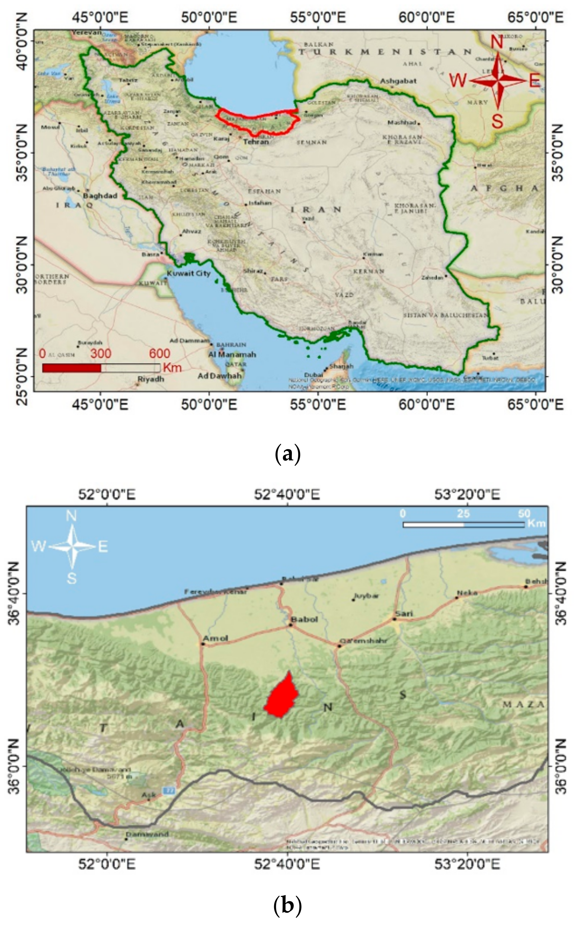
2.1. Study Area
2.2. Landslide Inventory Data Preparation
2.3. Landslide Conditioning Factors
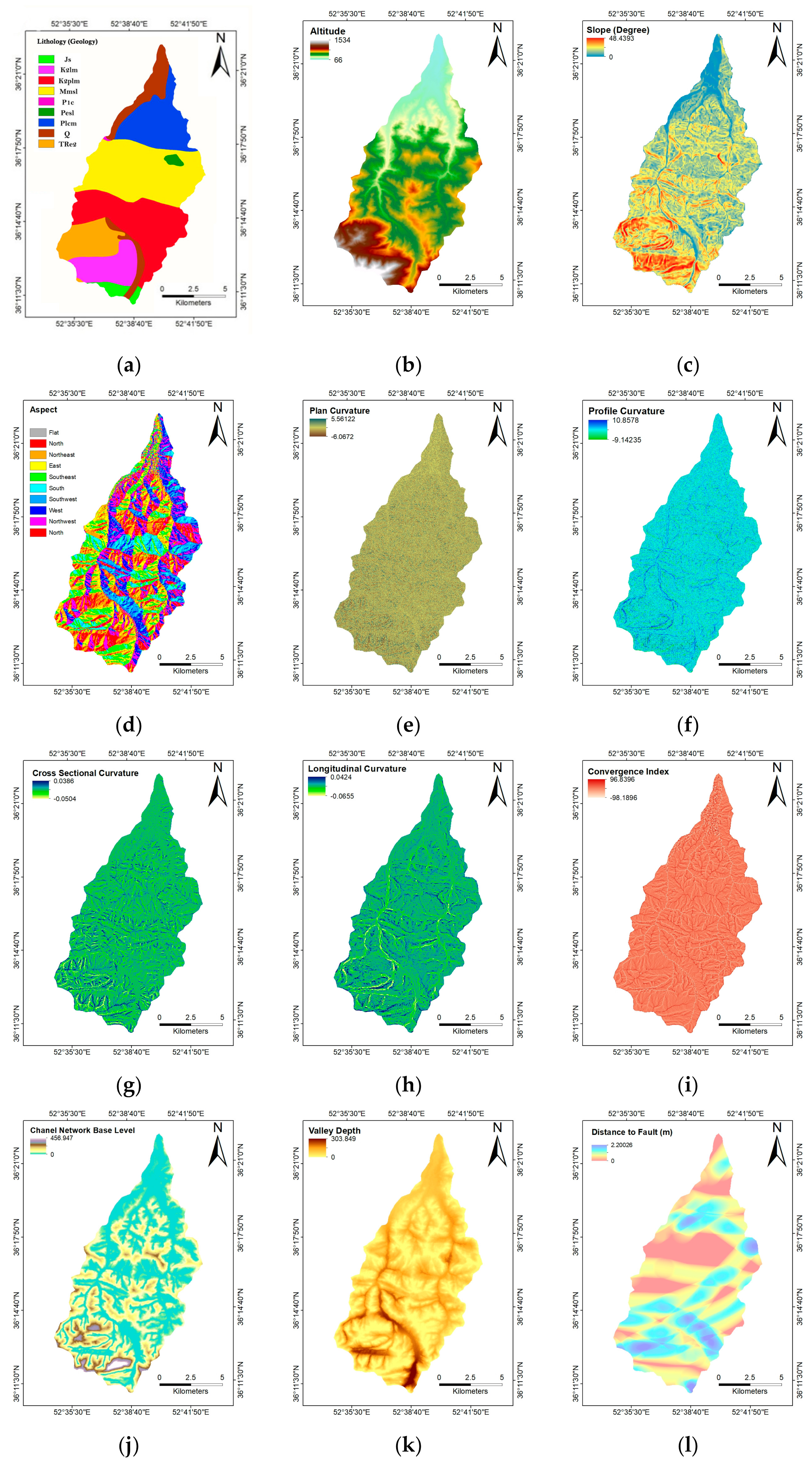
- Lithology (Geology): We used a 1:25,000-scale lithology (geology) map of the study area, which was obtained from the Geological Survey of Iran using satellite imagery. The dominant lithological units (e.g., sandstone and silty marl, mudstone, marly limestone and so on) in the area were classified into 9 classes, as per Figure 3a. Lithology (geology) was chosen, as it can be indicative of soil characteristics. These characteristics can be diverse and may influence erosion, ground stability and slide occurrence [17,35]. Table 1 shows the lithology (geology) of the Sajadrood catchment.
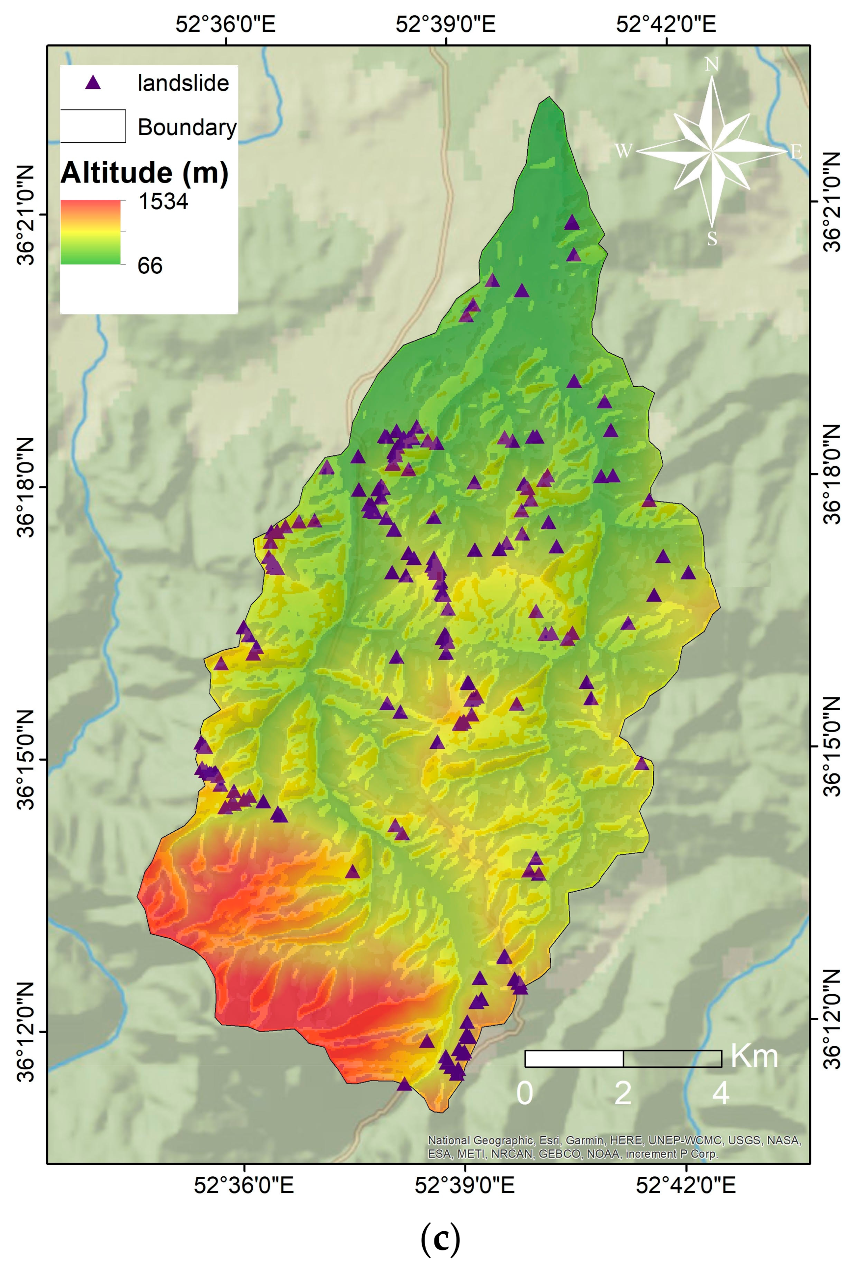
- Elevation and Topographical Data: We used a 1:25,000-scale topographic map of Sajarood to generate a 10 m Digital Elevation Model (DEM). The topographic map was provided by the National Cartographic Center of Iran from the aerial photogrametry. Since DEM derivatives can be utilized for geomorphological studies [38], first and second order DEM derivatives such as altitude, slope, aspect, cross sectional curvature, profile curvature, plan curvature, longitudinal curvature, convergence index, channel network base, and valley depth [39] can be very useful. We extracted them using SAGA GIS.
- Slope and Aspect: Both these CFs were generated from the study area’s DEM. For this study, the slope map was extracted to a maximum slope of 48° (Figure 3c). Aspect, which relates to meteorological and morphological characteristics, represents the horizontal direction of mountain slope faces [41]. The aspect map (Figure 3d) was divided into nine separate categories: (i) north, (ii) northeast, (iii) northwest, (iv) flat, (v) south, (vi) southeast, (vii) east, (viii) west and (ix) southwest. These two CFs were chosen, since slope directly influences the soil strength, and consequently, the landslide [42].
- Curvatures: Plan and profile curvatures are the descending flow acceleration (erosion/deposition rate) and the flow velocity variation of a slope, respectively [17]. Cross-sectional curvature, on the other hand, measures curvature perpendicular to the down slope direction to detect concave features such as channels (intersecting with the plan of slope normal and perpendicular to aspect direction). Longitudinal curvature calculates the curvature in the down slope direction (intersecting curvature with the plan of slope normal and aspect direction) [38,43]. For this research, plan curvature, profile curvature, cross-sectional curvature, and longitudinal curvature (Figure 3e–h) were manually classified into three categories: concave, flat, and convex shaped curvatures. More details and formulas regarding to curvatures are provided by Ehsani and Malekian [38], and Alkhasawneh et al [43].
- The Convergence Index: As another DEM derivative, the convergence index provides assessment of slope curvature (Figure 3i). This index describes the mean of the slope directions of neighboring pixels from the direction of the central pixel [39], which effectively indicates whether a pixel is convergent or divergent.
- Channel Network Base and Valley depth: Valleys and channels are considered as geomorphologic and hydrologic attributes [44]. The channel network base (Figure 3j) and valley depth (Figure 2) appear to influence landslides and debris flows distribution [45]. The channel network base uses elevation, flow direction, and divergence to calculate the network (http://www.saga-gis.org/saga_tool_doc/2.2.0/ta_channels_0.html). Valley depth contributes to drainage, that leads the way for the landslide. Therefore, it is based on the vertical distance to the depth contour lines (convergent) seen from the mountain ridges [44,45,46]. This can be estimated by subtracting the base level of the channel network from the DEM [47].
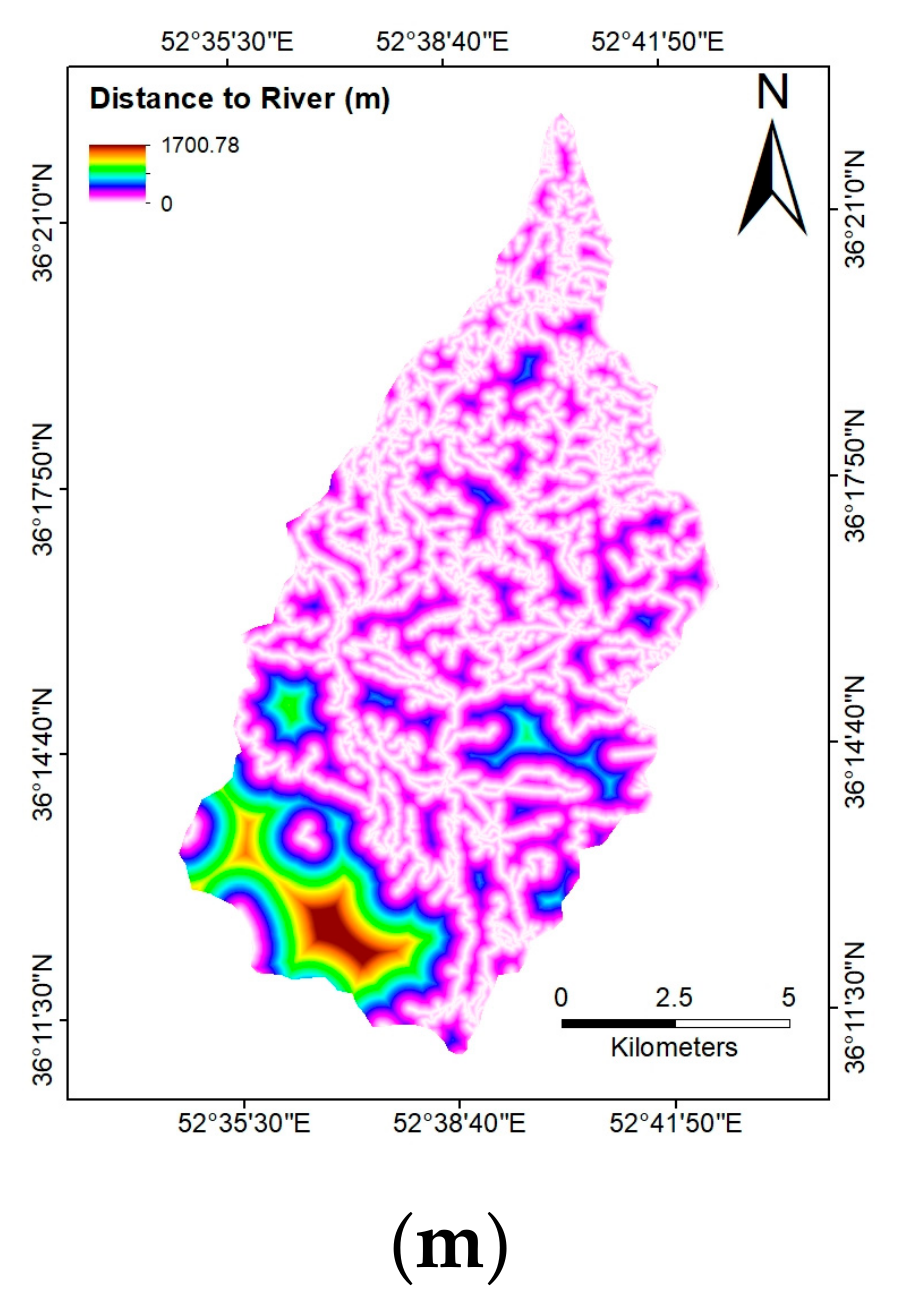
- Distance to Fault and Distance to River: From the topographic map, distance to fault and distance to river are generated based on the Euclidean distance function in ArcGIS (Figure 3l,m). These distances were chosen as landslides occurrence is most probable along the fault and river, due to erosion and ground instability [5,17,21].
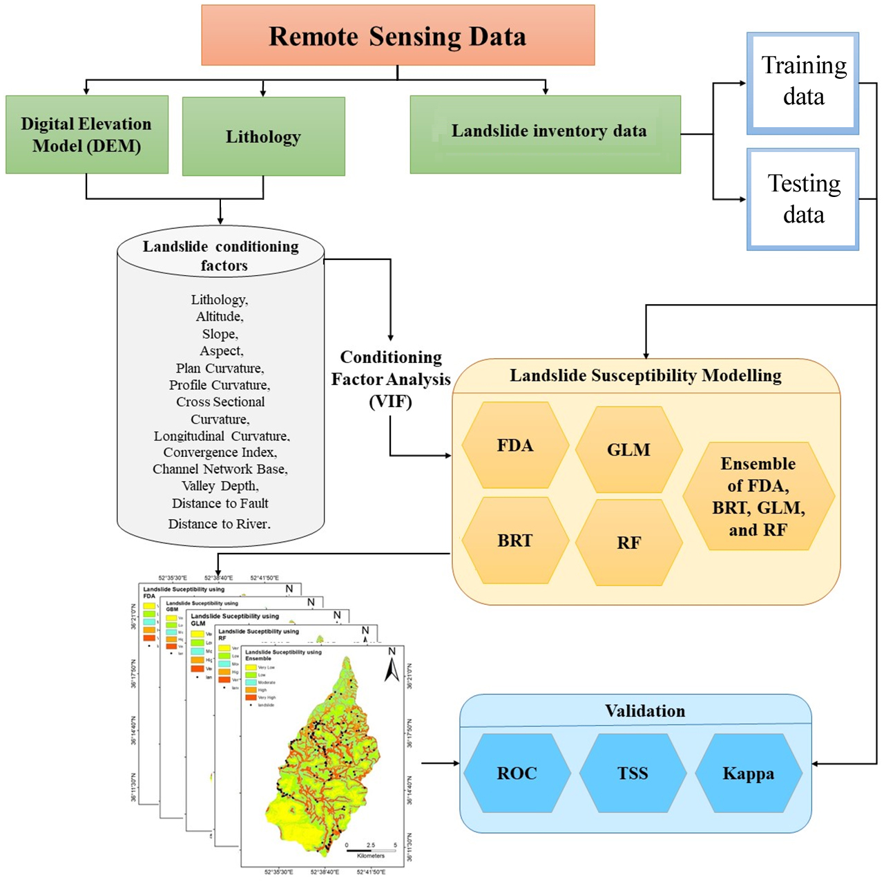
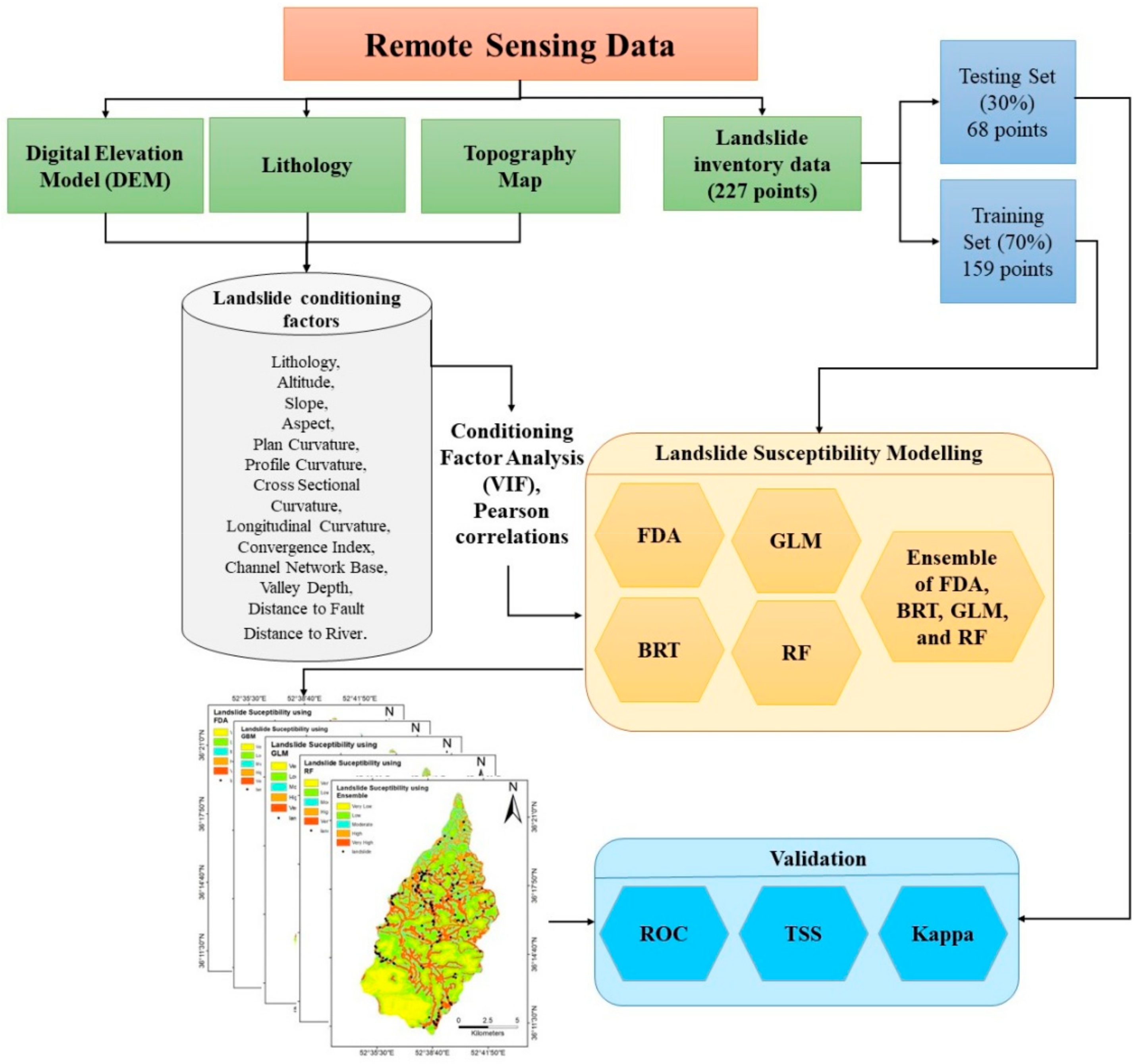
3. Methodology
3.1. Overview
3.2. Landslide Conditioning Factor Analysis
3.2.1. Variance Inflation Factor (VIF)
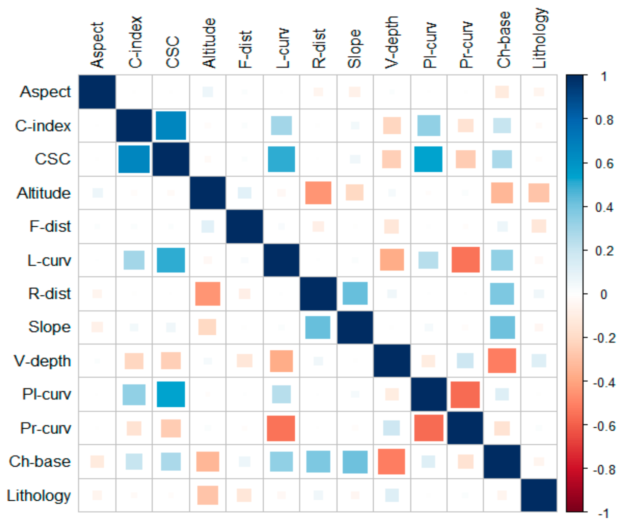
3.2.2. Pearson Correlations
3.3. Machine Learning Algorithms
3.3.1. Flexible Discriminant Analysis (FDA)
3.3.2. Generalized Linear Models (GLM)
3.3.3. Generalized Boosted Regression Models (GBM) or Boosted Regression Trees (BRT)
3.3.4. Random Forest (RF)
3.3.5. Ensemble of FDA, GBM (BRT), GLM, and RF
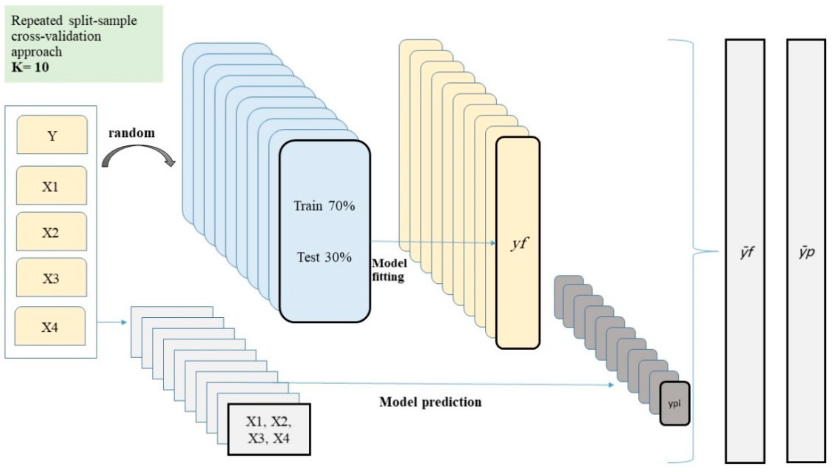
3.4. Model Validation
4. Results
5. Discussion
6. Conclusions
Author Contributions
Funding
Acknowledgments
Conflicts of Interest
References
- Cheng, Y.; Zhou, K.; Wang, J.; Yan, J. Big Earth Observation Data Integration in Remote Sensing Based on a Distributed Spatial Framework. Remote Sens. 2020, 12, 972. [Google Scholar] [CrossRef]
- Sedona, R.; Cavallaro, G.; Jitsev, J.; Strube, A.; Riedel, M.; Benediktsson, J.A. Remote sensing big data classification with high performance distributed deep learning. Remote Sens. 2019, 11, 3056. [Google Scholar] [CrossRef]
- Shirzadi, A.; Soliamani, K.; Habibnejhad, M.; Kavian, A.; Chapi, K.; Shahabi, H.; Chen, W.; Khosravi, K.; Pham, B.T. Shallow Landslide Susceptibility Mapping. Sensors 2018, 18, 3777. [Google Scholar] [CrossRef]
- Al-Najjar, H.A.H.; Kalantar, B.; Pradhan, B.; Saeidi, V. Conditioning Factor Determination for Mapping and Prediction of Landslide Susceptibility Using Machine Learning Algorithms. In Proceedings of the SPIE Remote Sensing 2019, Strasbourg, France, 10–12 September 2019; Volume 11156. [Google Scholar]
- Jebur, M.N.; Pradhan, B.; Tehrany, M.S. Optimization of landslide conditioning factors using very high-resolution airborne laser scanning (LiDAR) data at catchment scale. Remote Sens. Environ. 2014, 152, 150–165. [Google Scholar] [CrossRef]
- Shahabi, H.; Hashim, M. Landslide susceptibility mapping using GIS-based statistical models and Remote sensing data in tropical environment. Sci. Rep. 2015, 5, 1–15. [Google Scholar] [CrossRef] [PubMed]
- Dou, J.; Bui, D.T.; Yunus, A.P.; Jia, K.; Song, X.; Revhaug, I.; Xia, H.; Zhu, Z. Optimization of causative factors for landslide susceptibility evaluation using remote sensing and GIS data in parts of Niigata, Japan. PLoS ONE 2015, 10, e0133262. [Google Scholar] [CrossRef]
- Chang, Z.; Du, Z.; Zhang, F.; Huang, F.; Chen, J.; Li, W.; Guo, Z. Landslide susceptibility prediction based on remote sensing images and GIS: Comparisons of supervised and unsupervised machine learning models. Remote Sens. 2020, 12, 502. [Google Scholar] [CrossRef]
- Ma, Z.; Qin, S.; Cao, C.; Lv, J.; Li, G.; Qiao, S.; Hu, X. The influence of different knowledge-driven methods on landslide susceptibility mapping: A case study in the Changbai Mountain Area, Northeast China. Entropy 2019, 21, 372. [Google Scholar] [CrossRef]
- Pradhan, B.; Seeni, M.I.; Kalantar, B. Performance Evaluation and Sensitivity Analysis of Expert-Based, Statistical, Machine Learning, and Hybrid Models for Producing Landslide Susceptibility Maps; Springer: Cham, Switzerland, 2017; ISBN 9783319553429. [Google Scholar]
- Mahalingam, R.; Olsen, M.J.; Banion, M.S.O. Evaluation of landslide susceptibility mapping techniques using lidar-derived conditioning factors (Oregon case study). Geomat. Nat. Hazards Risk 2016, 5705. [Google Scholar] [CrossRef]
- Lee, S.; Evangelista, D.G. Landslide susceptibility mapping using probability and statistics models in Baguio City, Philippines. In Proceedings of the ISPRS 31st International Symposium on Remote Sensing of Environment, Saint Petersburg, Russia, 20–24 May 2005; pp. 20–24. [Google Scholar]
- Goetz, J.N.; Brenning, A.; Petschko, H.; Leopold, P. Evaluating machine learning and statistical prediction techniques for landslide susceptibility modeling. Comput. Geosci. 2015, 81, 1–11. [Google Scholar] [CrossRef]
- Afungang, R.N.; de Meneses Bateira, C.V.; Nkwemoh, C.A. Assessing the spatial probability of landslides using GIS and informative value model in the Bamenda highlands. Arab. J. Geosci. 2017, 10, 1–15. [Google Scholar] [CrossRef]
- Chen, W.; Pourghasemi, H.R.; Zhao, Z. A GIS-based comparative study of Dempster-Shafer, logistic regression and artificial neural network models for landslide susceptibility mapping. Geocarto Int. 2017, 6049, 1–19. [Google Scholar] [CrossRef]
- Mousavi, S.Z.; Kavian, A.; Soleimani, K.; Mousavi, S.R.; Shirzadi, A. GIS-based spatial prediction of landslide susceptibility using logistic regression model. Geomat. Nat. Hazards Risk 2011, 2, 33–50. [Google Scholar] [CrossRef]
- Kalantar, B.; Pradhan, B.; Amir Naghibi, S.; Motevalli, A.; Mansor, S. Assessment of the effects of training data selection on the landslide susceptibility mapping: A comparison between support vector machine (SVM), logistic regression (LR) and artificial neural networks (ANN). Geomat. Nat. Hazards Risk 2018, 9, 49–69. [Google Scholar] [CrossRef]
- Chen, W.; Pourghasemi, H.R.; Naghibi, S.A. Prioritization of landslide conditioning factors and its spatial modeling in Shangnan County, China using GIS-based data mining algorithms. Bull. Eng. Geol. Environ. 2018, 77, 611–629. [Google Scholar] [CrossRef]
- Kim, J.; Lee, S.M.; Jung, H.S.; Lee, S. Landslide Susceptibility Mapping using Random Forest and Boosted Tree Models in Pyeong-Chang, Korea. Geocarto Int. 2018, 33. [Google Scholar] [CrossRef]
- Hong, H.; Xu, C.; Chen, W. Providing a Landslide Susceptibility Map in Nancheng County, China, by Implementing Support Vector Machines. Am. J. Geogr. Inf. Syst. 2017, 6, 1–13. [Google Scholar]
- Tsangaratos, P.; Ilia, I. Comparison of a logistic regression and Naïve Bayes classifier in landslide susceptibility assessments: The influence of models complexity and training dataset size. Catena 2016, 145, 164–179. [Google Scholar] [CrossRef]
- Binh, T.P.; Indra, P.; Khabat, K.; Kamran, C.; Trong, T.P.; Quoc, N.T.; Vrya, H.S.; Tien, B.D. A Comparison of Support Vector Machines and Bayesian Algorithms for Landslide Susceptibility Modeling A Comparison of Support Vector Machines and Bayesian Algorithms for Landslide Susceptibility Modeling. Geocarto Int. 2018, 34, 1385–1407. [Google Scholar]
- Naghibi, S.A.; Pourghasemi, H.R. A comparative assessment between three machine learning models and their performance comparison by bivariate and multivariate statistical methods in groundwater potential mapping. Water Resour. Manag. 2015, 29, 5217–5236. [Google Scholar] [CrossRef]
- Gangappa, M.; Kiran, C.; Sammulal, P. Techniques for Machine Learning based Spatial Data Analysis: Research Directions. Int. J. Comput. Appl. 2017, 170, 9–13. [Google Scholar] [CrossRef]
- Goetz, J.N.; Guthrie, R.H.; Brenning, A. Integrating physical and empirical landslide susceptibility models using generalized additive models. Geomorphology 2011, 129, 376–386. [Google Scholar] [CrossRef]
- Youssef, A.M.; Pourghasemi, H.R.; Pourtaghi, Z.S.; Al-Katheeri, M.M. Landslide susceptibility mapping using random forest, boosted regression tree, classification and regression tree, and general linear models and comparison of their performance at Wadi Tayyah Basin, Asir Region, Saudi Arabia. Landslides 2015, 13, 1315–1318. [Google Scholar] [CrossRef]
- Hastie, T.; Tibshirani, R.; Buja, A.; Hastie, T.; Tibshirani, R.; Buja, A. Flexible Discriminant Analysis by Optimal Scoring. J. Am. Stat. Assoc. 1994, 89, 1255–1270. [Google Scholar] [CrossRef]
- Naghibi, S.A.; Pourghasemi, H.R.; Abbaspour, K. A comparison between ten advanced and soft computing models for groundwater qanat potential assessment in Iran using R and GIS. Theor. Appl. Climatol. 2018, 131, 967–984. [Google Scholar] [CrossRef]
- Peng, H. SVM-Flexible Discriminant Analysis; NC State University Department of Statistics: Raleigh, NC, USA, 2014. [Google Scholar]
- Solberg, A.H.S. Texture fusion and classification based on flexible discriminant analysis. In Proceedings of the 13th International Conference on Pattern Recognition, Vienna, Austria, 25–29 August 1996; pp. 596–600. [Google Scholar]
- Nguyen, P.T.; Tuyen, T.T.; Shirzadi, A.; Pham, B.T. Development of a Novel Hybrid Intelligence Approach for Landslide Spatial Prediction. Appl. Sci. 2019, 9, 2824. [Google Scholar] [CrossRef]
- Kordestani, M.D.; Naghibi, S.A.; Hashemi, H.; Ahmadi, K.; Kalantar, B. Groundwater potential mapping using a novel data-mining ensemble model. Hydrogeol. J. 2018, 27, 211–224. [Google Scholar] [CrossRef]
- Pham, B.T.; Tien Bui, D.; Prakash, I.; Dholakia, M.B. Hybrid integration of Multilayer Perceptron Neural Networks and machine learning ensembles for landslide susceptibility assessment at Himalayan area (India) using GIS. Catena 2017, 149, 52–63. [Google Scholar] [CrossRef]
- Fang, Z.; Wang, Y.; Peng, L.; Hong, H. Integration of convolutional neural network and conventional machine learning classifiers for landslide susceptibility mapping. Comput. Geosci. 2020, 139, 104470. [Google Scholar] [CrossRef]
- Mancini, F.; Ceppi, C.; Ritrovato, G. GIS and statistical analysis for landslide susceptibility mapping in the Daunia area, Italy. Nat. Hazards Earth Syst. Sci. 2010, 10, 1851–1864. [Google Scholar] [CrossRef]
- Umar, Z.; Pradhan, B.; Ahmad, A.; Jebur, M.N.; Tehrany, M.S. Earthquake induced landslide susceptibility mapping using an integrated ensemble frequency ratio and logistic regression models in West Sumatera Province, Indonesia. Catena 2014, 118, 124–135. [Google Scholar] [CrossRef]
- James, G.; Witten, D.; Hastie, T.; Tibshirani, R. An Introduction to Statistical Learning; Springer: Berlin/Heidelberg, Germany, 2013. [Google Scholar]
- Ehsani, A.; Malekian, A. Landforms identification using neural network-self organizing map and SRTM data. Desert 2012, 16, 111–122. [Google Scholar]
- Taner San, B. An evaluation of SVM using polygon-based random sampling in landslide susceptibility mapping: The Candir catchment area (western Antalya, Turkey). Int. J. Appl. Earth Obs. Geoinf. 2014, 26, 399–412. [Google Scholar]
- Sezer, E.A.; Pradhan, B.; Gokceoglu, C. Manifestation of an adaptive neuro-fuzzy model on landslide susceptibility mapping: Klang valley, Malaysia. Expert Syst. Appl. 2011, 38, 8208–8219. [Google Scholar] [CrossRef]
- Youssef, A.M.; Pradhan, B.; Pourghasemi, H.R.; Abdullahi, S. Landslide susceptibility assessment at Wadi Jawrah Basin, Jizan region, Saudi Arabia using two bivariate models in GIS. Geosci. J. 2015, 19, 449–469. [Google Scholar] [CrossRef]
- Park, S.; Kim, J. Landslide Susceptibility Mapping Based on Random Forest and Boosted Regression Tree Models, and a Comparison of Their Performance. Appl. Sci. 2019, 9, 942. [Google Scholar] [CrossRef]
- Alkhasawneh, M.S.; Ngah, U.K.; Tay, L.T.; Isa, N.A.M.; Al-batah, M.S. Determination of Important Topographic Factors for Landslide Mapping Analysis Using MLP Network. Sci. World J. 2013, 2013, 1–12. [Google Scholar] [CrossRef]
- Hooshyar, M.; Wang, D.; Kim, S.; Medeiros, S.C.; Hagen, S.C. Valley and channel networks extraction based on local topographic curvature and k-means clustering of contours. Water Resour. Res. 2016, 52, 8081–8102. [Google Scholar] [CrossRef]
- Märker, M.; Hochschild, V.; Maca, V.; Vilímek, V. Stochastic assessment of landslides and debris flows in the Jemma basin, Blue Nile, Central Ethiopia. Geogr. Fis. Din. Quat. 2016, 39, 51–58. [Google Scholar]
- Meinhardt, M.; Fink, M.; Tünschel, H. Landslide susceptibility analysis in central Vietnam based on an incomplete landslide inventory: Comparison of a new method to calculate weighting factors by means of bivariate statistics. Geomorphology 2015, 234, 80–97. [Google Scholar] [CrossRef]
- Lee, S.; Lee, M.; Jung, H. Data Mining Approaches for Landslide Susceptibility Mapping in Umyeonsan, Seoul, South Korea. Appl. Sci. 2017, 7, 683. [Google Scholar] [CrossRef]
- Tehrany, M.S.; Jones, S.; Shabani, F. Identifying the essential flood conditioning factors for flood prone area mapping using machine learning techniques. Catena 2019, 175, 174–192. [Google Scholar] [CrossRef]
- Naimi, B. usdm: Uncertainty Analysis for Species Distribution Models, version 1.1–18; 2016. Available online: https://CRAN.R-project.org/package=usdm (accessed on 27 May 2020).
- Kalantar, B.; Ueda, N.; Lay, U.S.; Al-Najjar, H.A.H.; Halin, A.A. Conditioning Factors Determination for Landslide Susceptibility Mapping using Support Vector Machine Learning. In Proceedings of the 2019 IEEE International Geoscience and Remote Sensing Symposium, Yokohama, Japan, 28 July–2 August 2019; pp. 9626–9629. [Google Scholar]
- Roy, J.; Saha, S. Landslide susceptibility mapping using knowledge driven statistical models in Darjeeling District, West Bengal, India. Geoenviron. Disasters 2019, 6. [Google Scholar] [CrossRef]
- Flury, B.; Riedwyl, H. Using Multivariate Statistics, 3rd ed.; HarperCollins: New York, NY, USA, 1996. [Google Scholar]
- Hastie, T.; Tibshirani, R. Discriminant Analysis by Gaussian Mixtures. J. R. Stat. Soc. Ser. B 1996, 58, 155–176. [Google Scholar] [CrossRef]
- Li, X.; Wang, Y. Applying various algorithms for species distribution modelling. Integr. Zool. 2013, 8, 124–135. [Google Scholar] [CrossRef]
- Naghibi, S.A.; Pourghasemi, H.R.; Dixon, B. GIS-based groundwater potential mapping using boosted regression tree, classification and regression tree, and random forest machine learning models in Iran. Environ. Monit. Assess. 2016, 188, 1–27. [Google Scholar] [CrossRef]
- Chehata, N.; Guo, L.; Mallet, C. Airborne lidar feature selection for urban classification using random forests. In Proceedings of the ISPRS Workshop: Laserscanning 09, Paris, France, 1–2 September 2009; pp. 207–212. [Google Scholar]
- Eisavi, V.; Homayouni, S.; Yazdi, A.M.; Alimohammadi, A. Land cover mapping based on random forest classification of multitemporal spectral and thermal images. Environ. Monit. Assess. 2015, 187, 1–14. [Google Scholar] [CrossRef]
- Thuiller, W. BIOMOD—Optimizing predictions of species distributions and projecting potential future shifts under global change. Glob. Chang. Biol. 2003, 9, 1353–1362. [Google Scholar] [CrossRef]
- Pham, B.T.; Jaafari, A.; Prakash, I.; Bui, D.T. A novel hybrid intelligent model of support vector machines and the MultiBoost ensemble for landslide susceptibility modeling. Bull. Eng. Geol. Environ. 2019, 78, 2865–2886. [Google Scholar]
- Araújo, M.B.; New, M. Ensemble forecasting of species distributions. Trends Ecol. Evol. 2007, 22, 42–47. [Google Scholar] [CrossRef]
- Burnham, K.P.; Anderson, D.R.; Huyvaert, K.P. AIC model selection and multimodel inference in behavioral ecology: Some background, observations, and comparisons. Behav. Ecol. Sociobiol. 2002, 65, 23–35. [Google Scholar] [CrossRef]
- Swets, J.A. Measuring the accuracy of diagnostic systems. Science 1988, 240, 1285–1293. [Google Scholar] [CrossRef] [PubMed]
- Allouche, O.; Tsoar, A.; Kadmon, R. Assessing the accuracy of species distribution models: Prevalence, kappa and the true skill statistic (TSS). J. Appl. Ecol. 2006, 1223–1232. [Google Scholar] [CrossRef]
- Ruete, A.; Leynaud, G.C. Goal-oriented evaluation of species distribution models’ accuracy and precision: True Skill Statistic profile and uncertainty maps. PeerJ Prepr. 2015, 3, e1208v1. [Google Scholar] [CrossRef]
- Naghibi, S.A.; Moghaddam, D.D.; Kalantar, B.; Pradhan, B.; Kisi, O. A comparative assessment of GIS-based data mining models and a novel ensemble model in groundwater well potential mapping. J. Hydrol. 2017, 548, 471–483. [Google Scholar] [CrossRef]
- Arabameri, A.; Pradhan, B.; Rezaei, K.; Sohrabi, M.; Kalantari, Z. GIS-based landslide susceptibility mapping using numerical risk factor bivariate model and its ensemble with linear multivariate regression and boosted regression tree algorithms. J. Mt. Sci. 2019, 16, 595–618. [Google Scholar] [CrossRef]
- Districts, K.; Bengal, W.; Bui, D.T. A Novel Ensemble Approach for Landslide Susceptibility Mapping (LSM) in Darjeeling and Kalimpong Districts, West Bengal, India. Remote Sens. 2019, 11, 2866. [Google Scholar] [CrossRef]


| Symbol | Lithology (Geology) |
|---|---|
| Js | Shale with Intercalations of Conglomerate, Sandstone, Radiolarite, limestone and Volcanics |
| Mmsl | Marl, Calcareous Sandstone, Sandy Limestone, and minor Conglomerate |
| K2lm | Pale—Red Marl, Gypsiferous Marl and Limestone |
| P1c | Polymictic Conglomerate and Sandstone |
| Q | Low Level Piedment Fan and Vally Terrace Deposits |
| Plcm | Marl, Shale, Sandstone and Conglomerate |
| TRe2= PeEm | Marl and Gypsiferous Marl Locally Gypsiferous Mudstone |
| Pesl | Sandstone, Calcareous Shale and Mudstone |
| K2lm | Hyporite Bearing Limestone |
| Conditioning Factors | VIF |
|---|---|
| Lithology | 2.26334 |
| Altitude | 1.321653 |
| Longitudinal Curvature | 1.531395 |
| Profile Curvature | 1.463843 |
| Plan Curvature | 1.463843 |
| Distance to River | 1.600335 |
| Slope | 1.391226 |
| Valley Depth | 1.695373 |
| Aspect | 1.024332 |
| Channel Network Base Level | 2.31 |
| Convergence Index | 1.834950 |
| Cross Sectional Curvature | 2.240171 |
| Distance to Fault | 2.514229 |
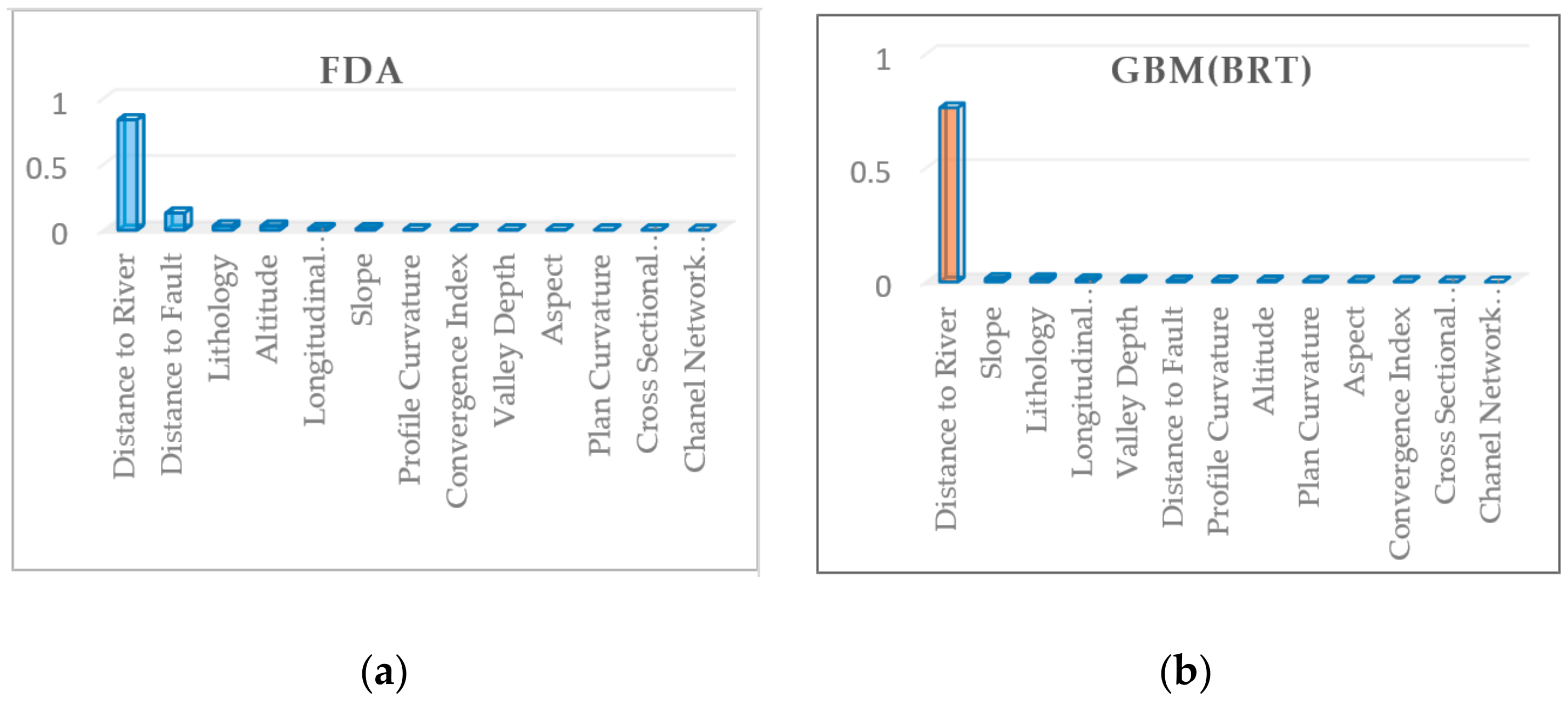
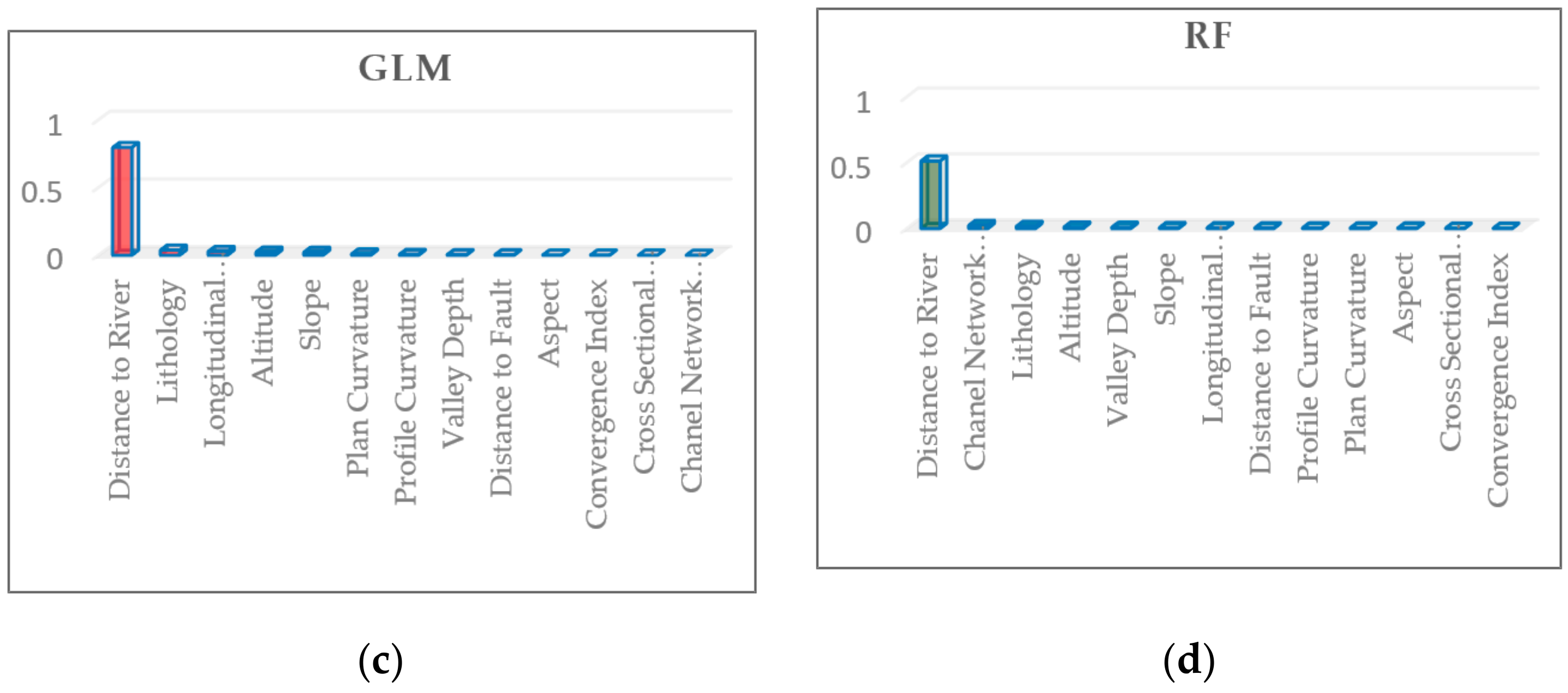
| Conditioning Factors | FDA | GBM(BRT) | GLM | RF |
|---|---|---|---|---|
| Lithology | 0.03313 | 0.01437 | 0.03793 | 0.01674 |
| Altitude | 0.03125 | 0.00496 | 0.02332 | 0.0107 |
| Longitudinal Curvature | 0.01239 | 0.00954 | 0.0283 | 0.0058 |
| Profile Curvature | 0.0036 | 0.00546 | 0.00661 | 0.00457 |
| Plan Curvature | 0.00169 | 0.0042 | 0.00966 | 0.00451 |
| Distance to River | 0.83677 | 0.76437 | 0.79594 | 0.51263 |
| Slope | 0.01063 | 0.01501 | 0.02247 | 0.00693 |
| Valley Depth | 0.00213 | 0.00743 | 0.00456 | 0.00939 |
| Aspect | 0.00209 | 0.00375 | 0.00148 | 0.00435 |
| Channel Network Base Level | 0 | 0 | 0 | 0.02343 |
| Convergence Index | 0.00277 | 0.00334 | 0.00123 | 0.00226 |
| Cross Sectional Curvature | 0.00148 | 0.00192 | 0.00066 | 0.00235 |
| Distance to Fault | 0.1301 | 0.00572 | 0.00373 | 0.00528 |
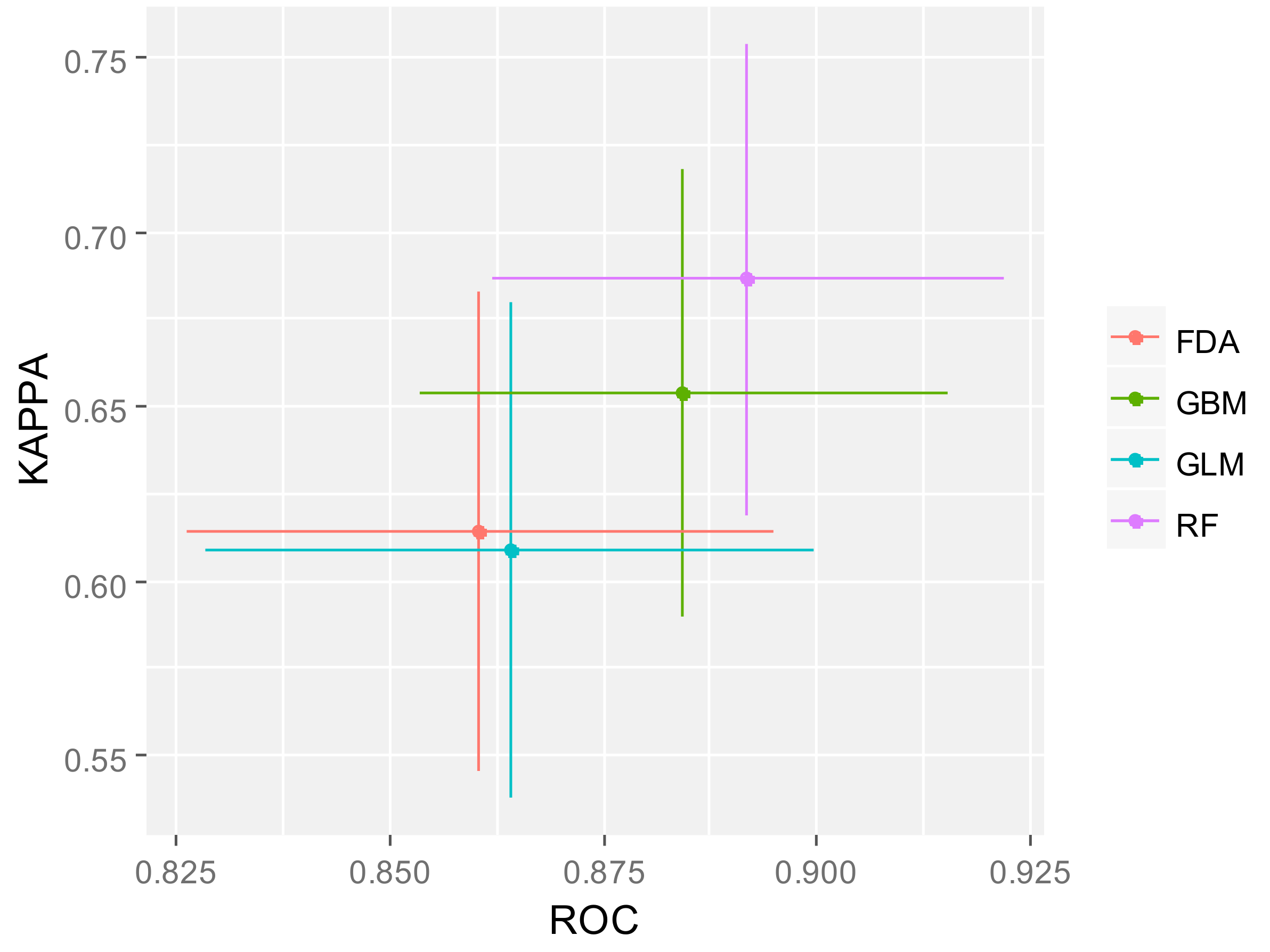
| Dataset | FDA | GBM (BRT) | GLM | RF | Ensemble | |||||
|---|---|---|---|---|---|---|---|---|---|---|
| avg | S.d | avg | S.d | avg | S.d | avg | S.d | avg | S.d | |
| TSS | 0.614 | 0.0682 | 0.6551 | 0.0636 | 0.6096 | 0.0704 | 0.6869 | 0.0674 | 0.6986 | 0.0207 |
| ROC | 0.860 | 0.0343 | 0.8842 | 0.0309 | 0.8641 | 0.0357 | 0.8919 | 0.0300 | 0.9043 | 0.0148 |
| Kappa | 0.614 | 0.0688 | 0.6538 | 0.0641 | 0.6086 | 0.0710 | 0.6867 | 0.0676 | 0.6915 | 0.0204 |
| Sensitivity | 80.00 | 0.074 | 84.44 | 0.061 | 71.11 | 0.072 | 86.66 | 0.063 | 86.44 | 0.022 |
| Specificity | 82.22 | 0.065 | 80.00 | 0.053 | 84.44 | 0.073 | 84.44 | 0.061 | 84.22 | 0.024 |
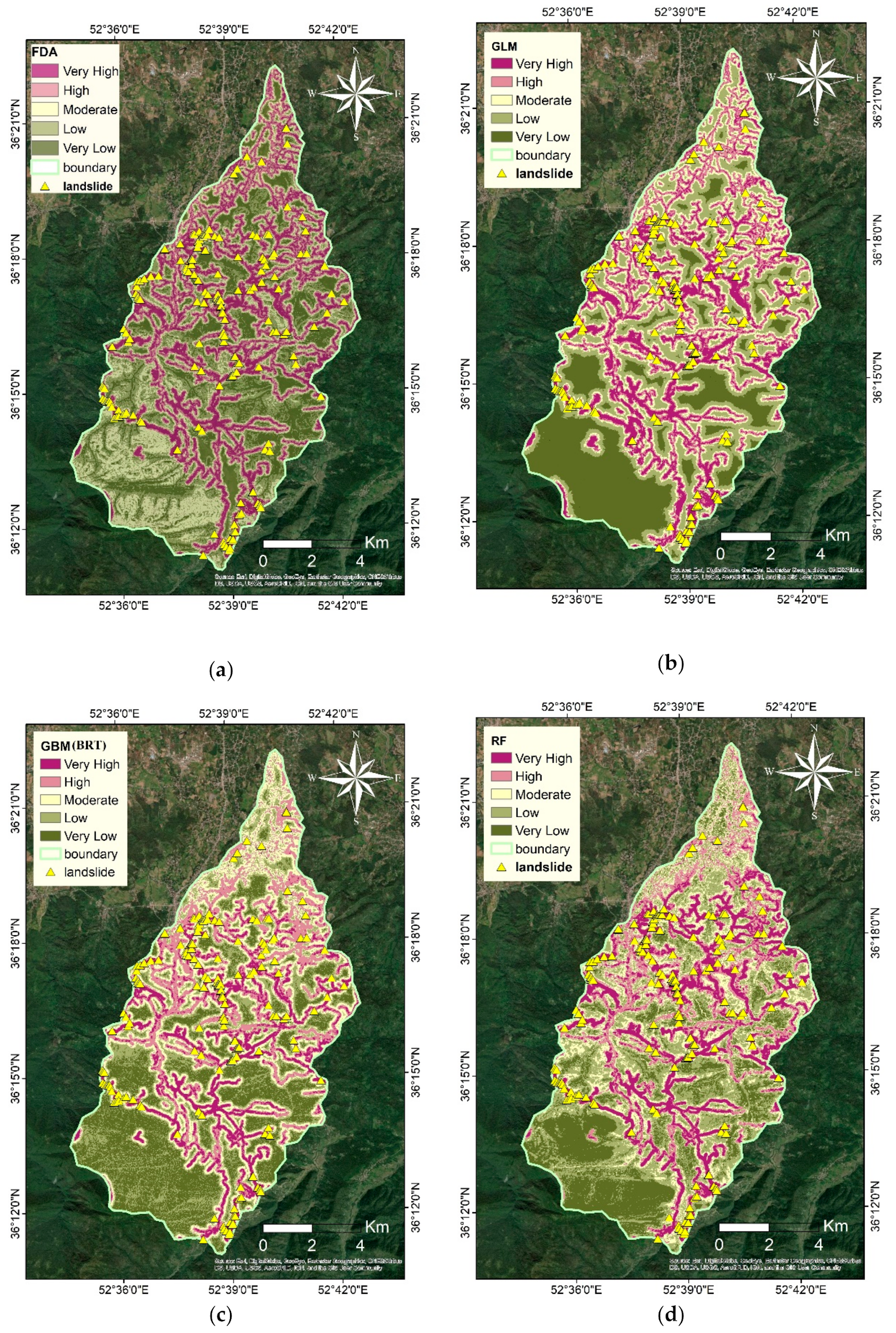
| Susceptibility | Models | |||||||||
|---|---|---|---|---|---|---|---|---|---|---|
| FDA | GLM | GBM (BRT) | RF | Ensemble | ||||||
| % | Area (ha) | % | Area (ha) | % | Area (ha) | % | Area (ha) | % | Area (ha) | |
| Very Low | 59 | 7408 | 56.14 | 7011 | 69.51 | 8680 | 71.51 | 8930 | 64.42 | 8044 |
| Low | 11.5 | 1436.5 | 12.19 | 1523 | 4.63 | 579 | 6.57 | 821 | 9.96 | 1244 |
| Moderate | 10.7 | 1343 | 11.71 | 1463 | 4.32 | 540 | 6.04 | 755 | 7.25 | 906 |
| High | 12.9 | 1616 | 12.5 | 1561 | 6.45 | 806 | 6.18 | 772 | 8.97 | 1121 |
| Very High | 5.9 | 683 | 7.43 | 928.5 | 15.06 | 1881.5 | 9.67 | 1208.5 | 9.38 | 1171.5 |
© 2020 by the authors. Licensee MDPI, Basel, Switzerland. This article is an open access article distributed under the terms and conditions of the Creative Commons Attribution (CC BY) license (http://creativecommons.org/licenses/by/4.0/).
Share and Cite
Kalantar, B.; Ueda, N.; Saeidi, V.; Ahmadi, K.; Halin, A.A.; Shabani, F. Landslide Susceptibility Mapping: Machine and Ensemble Learning Based on Remote Sensing Big Data. Remote Sens. 2020, 12, 1737. https://doi.org/10.3390/rs12111737
Kalantar B, Ueda N, Saeidi V, Ahmadi K, Halin AA, Shabani F. Landslide Susceptibility Mapping: Machine and Ensemble Learning Based on Remote Sensing Big Data. Remote Sensing. 2020; 12(11):1737. https://doi.org/10.3390/rs12111737
Chicago/Turabian StyleKalantar, Bahareh, Naonori Ueda, Vahideh Saeidi, Kourosh Ahmadi, Alfian Abdul Halin, and Farzin Shabani. 2020. "Landslide Susceptibility Mapping: Machine and Ensemble Learning Based on Remote Sensing Big Data" Remote Sensing 12, no. 11: 1737. https://doi.org/10.3390/rs12111737
APA StyleKalantar, B., Ueda, N., Saeidi, V., Ahmadi, K., Halin, A. A., & Shabani, F. (2020). Landslide Susceptibility Mapping: Machine and Ensemble Learning Based on Remote Sensing Big Data. Remote Sensing, 12(11), 1737. https://doi.org/10.3390/rs12111737