Article

Combining Electrical Resistivity Tomography and Satellite Images for Improving Evapotranspiration Estimates of Citrus Orchards

by
Daniela Vanella
1,
Juan Miguel Ramírez-Cuesta
2,*,
Diego S. Intrigliolo
2 and
Simona Consoli
1
1
Dipartimento di Agricoltura, Alimentazione, Ambiente (Di3A), Università degli Studi di Catania, Via S. Sofia, 100–95123 Catania, Italy
2
Dpto. Riego, Centro de Edafología y Biología Aplicada del Segura (CEBAS-CSIC), P.O. Box 164, 30100 Murcia, Spain
*
Author to whom correspondence should be addressed.
Remote Sens. 2019, 11(4), 373; https://doi.org/10.3390/rs11040373
Submission received: 29 December 2018 / Revised: 3 February 2019 / Accepted: 11 February 2019 / Published: 13 February 2019
(This article belongs to the Special Issue Advances in the Remote Sensing of Terrestrial Evaporation)

Abstract

:
An adjusted satellite-based model was proposed with the aim of improving spatially distributed evapotranspiration (ET) estimates under plant water stress conditions. Remote sensing data and near surface geophysics information, using electrical resistivity tomography (ERT), were used in a revised version of the original dual crop coefficient (Kc) FAO-56 approach. Sentinel 2-A imagery were used to compute vegetation indices (VIs) required for spatially estimating ET. The potentiality of the ERT technique was exploited for tracking the soil wetting distribution patterns during and after irrigation phases. The ERT-derived information helped to accurately estimate the wet exposed fraction (few) and therefore the water evaporated from the soil surface into the dual Kc FAO-56 approach. Results, validated by site-specific ET measurements (ETEC) obtained using the eddy covariance (EC) technique, showed that ERT-adjusted ET estimates (ETERT) were considerably reduced (15%) when compared with the original dual Kc FAO-56 approach (ETFAO), soil evaporation overestimation being the main reason for these discrepancies. Nevertheless, ETFAO and ETERT showed overestimations of 64% and 40% compared to ETEC. This is because both approaches determine ET under standard conditions without water limitation, whereas EC is able to determine ET even under soil water deficit conditions. From the comparison between ETEC and ETERT, the water stress coefficient was experimentally derived, reaching a mean value for the irrigation season of 0.74. The obtained results highlight how new technologies for soil water status monitoring can be incorporated for improving ET estimations, particularly under drip irrigation conditions.

Graphical Abstract

1. Introduction

Soil surface evaporation (E) and crop transpiration (T) play a crucial role in terrestrial water balance. Their estimation results are critical for understanding crop water use efficiency (WUE) and improving decision-making for soil and crop water management [1,2,3]. In this sense, improving the methods used for determining these components (T and E) is needed. While T represents the water used directly by crops, E is considered as an unproductive portion of WUE, which can range from 10% [4] to 59% [5] of the seasonal water balance. In general, two strategies are addressed with the aim of enhancing WUE: (i) increase T or; (ii) reduce E losses. Numerous authors have proposed different mechanisms to increase the proportion of water that is transpired by crop rather than E losses, including: early sowing [6,7], enhancing crop vigorousness [8,9], using narrow row spacing [10], applying high plant densities [11], and adopting mulching, stubble retention, and a proper weed management [12,13].
Evapotranspiration (ET), which consists of the sum up of both T and E components, can be determined at different spatial and temporal resolutions through different techniques (e.g., lysimeter; eddy covariance, EC; scintillometry). However, partitioning among E and T components is not an easy task. For this reason, it is usual to resort to models, such as the FAO-56 approach [14], which is used as reference. This model includes a simple approach (single crop coefficient, Kc), where T and E are considered together, and a more complex methodology (dual Kc FAO-56), where both T and E components are determined separately (i.e., basal crop coefficient Kcb and evaporation coefficient Ke). Both models can be combined with spectral data provided using remote sensors in order to provide spatially distributed ET estimates [15]. Although Kcb represents a specific crop characteristics index that varies only to a limited extent with climate, Ke can vary considerably depending on the time interval between wetting events, the magnitude of the wetting event, and the E power of the atmosphere. Nevertheless, these aspects are not deeply addressed in the FAO-56 approach. Thus, the use of alternative techniques is required in order to obtain more accurate Ke estimates.
Moreover, the calculation of Ke needs to take into account the spatial and temporal distribution of irrigation-wetting patterns that are governed by static and dynamic conditions, such as soil characteristics (e.g., hydraulic parameters, texture, structure, initial water content), irrigation systems (types, emitter spacing, discharge rate, and irrigation frequency), and root distribution. In general, soil wetting patterns can be obtained using in situ soil water (SW) measurements. Caution needs to be applied on the use of SW measurements, since site conditions (compaction layers or surface soil conditions) may be quite site-specific, and installation of instrumentation can affect the soil wetting patterns being measured [16]. Undisturbed methods, such as dye tracers, often combined with flow and/or transport modeling, have been used to describe infiltration from a point/line source; however, models do not at present fully reflect the current state of process understanding and empirical knowledge of preferential flow [17]. A number of near surface geophysics methods have been adopted for image irrigation wetting patterns [18]. Among these minimally invasive methods, electrical resistivity tomography (ERT) has the main advantage of being sensitive in monitoring soil-plant interactions in terms of SW relationships with high-resolution scale both in two and/or three dimensions [19,20,21,22]. Furthermore, ERT can provide useful information on soil wetting patterns both spatially and temporally distributed if applied in time-lapse mode.
Therefore, the main objective of this work was to explore the potentialities of incorporating ERT derived surface wetting patterns into a satellite-based dual Kc FAO-56 approach for estimating E and assessing its influence on ET by comparison with EC measurements.

2. Materials and Methods

In this study, the assessment of an updated satellite-based procedure based on a dual Kc FAO-56 approach is proposed. A schematic summary of the adopted methodology is reported in Figure 1.
The original satellite dual Kc FAO-56 approach [14] was adjusted with ERT-derived data that provided site-specific information on the exposed wetting fraction (few). This parameter represents the fraction of soil that is both exposed and wetted (from which most evaporation occurs). As reported in [14], few contributes in the definition of the soil evaporation coefficient (Ke, Equation (2)) and as well in ET determination (see Equation (1)). ERT surveys provided few that was incorporated as a parameter into the soil water balance (SWB) model (Equation (4)) within the dual Kc FAO-56 approach, permitting the obtainment of an ERT-adjusted evaporation coefficient (Ke,ERT) and evapotranspiration estimates (ETERT).
A validation of ET estimates obtained using both the original dual Kc FAO-56 (ETFAO) and the ERT-adjusted model (ETERT) was performed with EC-based ET measurements (ETEC) collected in situ. In the following sub-sections, the materials and methods are described in detail.

2.1. Original Model Description

The original dual Kc FAO-56 approach determines crop evapotranspiration (ETFAO) based on the concepts of reference evapotranspiration (ET0) and separate coefficients for crop T (represented by the basal crop coefficient, Kcb) and E (Ke), as follows:
ET FAO = ( K cb + K e ) · ET 0
where ET0 (mm d−1) is estimated by using the Penman–Monteith equation with hourly weather data (see 1.2) supplied by a weather station located close to the study site.
Ke depends on the water available in the surface layer of the topsoil and its estimation requires a daily water balance (SWB) computation for the surface soil layer in order to determine the cumulative E or depletion from the wet condition, as follows:
K e = K r ( K c , max K cb )
where Kc,max is the maximum crop coefficient value following rain or irrigation while Kr represents the reduction applied to E depending on the amount of water evaporated from the soil, as follows:
K r = TEW D e , i TEW REW
where TEW = 1000 (θFC − 0.5 θWP) Ze is the total evaporable water (i.e., maximum depth of water that can be evaporated from the soil surface layer), with θFC and θFC measured soil field capacity and wilting point (see 2.3) at the study site and Ze equal to 0.1, as reported in [14]; REW is the readily evaporable water (fixed at 10 mm for the study site soil, i.e., sandy loam [14]); and De,i is the cumulative depth of evaporation from the topsoil (mm) at the end of the 1-th day, and it is solved as follows:
D e , i = D e , i 1 ( P i RO i ) I i f w + E i f ew + T ew , i + DP e , i
where De,i−1 is the cumulative depth of E following complete wetting from the exposed and wetted fraction of the topsoil at the end of day i − 1 (mm); Pi is precipitation on day i (mm); ROi is precipitation runoff from the soil surface on day i (mm); Ii is irrigation depth on day i that infiltrates the soil (mm); Ei is evaporation on day i (i.e., Ei = Ke ET0) (mm); Tew,i is depth of T from the exposed and wetted fraction of the soil surface layer on day i (mm); DPe,i is deep percolation loss from the topsoil layer on day i if SW exceeds θFC (mm); fw is the fraction of soil surface wetted by irrigation (0.35 for drip irrigation [14]); few is exposed and wetted soil fraction, computed as the lowest value between the average exposed soil fraction not covered (or shaded) by vegetation and fw [14]. Therefore, few calculation within the SWB depends also on the occurrence of irrigation and precipitation and it is calculated differently for each scenario as: (1) if the surface is wetted by irrigation, then fw is the fw for the irrigation system, and therefore few is equal to 0.35 (this value is obtained from [14]); (2) if the surface is wetted by significant rain (i.e., >3 to 4 mm) with no irrigation, fw = 1 and therefore few is (1 − fc); and (3) if there is neither irrigation nor significant precipitation, few is the few of the previous day. However, the value of 0.35 considered in this approach, as it is a general theoretical few procedure, may not reflect the site-specific conditions, which could be more accurately determined performing local measurements (as the ERT-adjustment described in Section 2.2 “ERT-adjusted model parameter”).

2.2. ERT-Adjusted Model Parameter

As stated in Section 2.1, few values proposed in [14] can be adjusted in order to account for the site specificities (such as soil type and depth, and dripper flow and density, among others). This is the case of the novel ERT-adjusted dual Kc FAO-56 approach proposed herein. In this approach, Kr,ERT (Equation (3)) and Ke,ERT (Equation (2)) were calculated by solving the SWB model (Equation (4)) using the few information provided by ERT instead of using the FAO-56 proposed few value as in the original FAO-56 model, thus ETERT was derived by including the modified Ke,ERT term in Equation (1).
ERT (see [23]) is an active source geophysical method that uses a low-frequency electrical current, galvanically injected into the ground between a pair of current source electrodes, and measures the potential between two or more different potential electrodes. A cross section or a volume distribution of electrically resistive or conductive regions in the subsurface is the result obtained by repeating the patterns through many combinations of transmitting and receiving electrodes along a line or grid (or with borehole electrodes). The current, voltage, electrode spacing, and electrode configuration are used to calculate the electrical resistivity (ER, i.e., the inverse of electrical conductivity).
ERT surveys were carried out in 2017 (15th and 18th September) at the experimental site. A three-dimensional (3-D) set-up (made of 72 surface and borehole electrodes) was used to monitor the unsaturated soil volume (1.3 × 1.3 × 1.2 m) around the root-zone of two trees, one irrigated by micro-drippers at full rate, T1, and the other one supplied at 50% of T1 by PRD strategy, T2. A full description of the 3-D ERT set-up and data processing is reported in [22].
The electrical resistance (ohm, Ω) dataset was collected at T1 and T2, with short-term repetitions during and after irrigation phases, in order to get dynamic information about sub-surface processes (for further details refer to [24]). Table 1 displays the acquisition time during the irrigation phase for T1 and T2.
Time-lapse inversions were adopted to produce images of ER changes (ER ratio in %) before, during, and after irrigation phase. These relative inversions (time-lapse) are calculated from ratios (dr, Equation (5)) between the electrical resistances collected before and after irrigation:
d r = d t d 0 · F ( σ ohm )
where dt and d0 are the electrical resistance values (Ω) at time t and time 0 (initial condition), and Fohm) is the electrical resistance (Ω), obtained by running the forward model for an arbitrary ER of 100 Ω m. This calculation was performed simultaneously for T1 and T2 using a 5% error level [22].
Soil wetting distribution patterns (i.e., surface and depth of the soil layer dried by E) were identified based on ER decreasing in respect to the initial condition (no irrigation) by applying a threshold corresponding to a reduction in ER equal to or greater than 10%.
The few parameter used to set the SWB model (Equation (4)) within the ERT-adjusted dual Kc FAO-56 approach was retrieved from the volume derived by ERT. From the entire volume, the ER ratio values corresponding uniquely to the first 10 cm were extracted, since it was assumed that it is mainly at this depth where soil evaporation occurs. Once the data corresponding to the first 10 cm were extracted, few was determined by recognizing the soil wetting patterns (i.e., extracting all the values corresponding to the fixed threshold) at the different acquisition times after the irrigation beginning (Figure 2a and Table 1). Finally, the constant few value used in the ERT-adjusted approach was obtained as an average of all instantaneous values retrieved in each acquisition time (Figure 2a and Table 1).

2.3. Satellite-Based Dual Kc Approach

The dual Kc FAO-56 approach (original and ERT-adjusted), applied in this study, incorporates data derived from remote sensing in order to obtain spatially distributed estimates of Ke (Ke,FAO and Ke,ERT), Kcb (Equations (2) and (6)), and ET (ETFAO and ETERT) (Equation (1)).
Sentinel 2-A (L-1C) data offered by the European Space Agency (ESA), with a spatial resolution of 10 m in the visible and near-infrared (VNIR) region and available every 10 days, were selected on the basis of clear sky condition and irrigation application.
Table 2 displays the dates of the satellite imagery used within the reference period June–September 2017.
Remote sensing data were used to determine Kcb (Equations (1) and (2)) as a function of the soil adjusted vegetation index (SAVI) following the methodology proposed by [25,26]:
K cb = K cb , max F c , max ( SAVI SAVI min SAVI max SAVI min )
where SAVImax and SAVImin refer to the maximum and minimum SAVI values for each image, and Fc,max is the maximum value of fractional vegetation cover (fc) within the study site for which Kcb reaches its maximum value (as in [14]).
The SAVI index is calculated as follows:
SAVI = ( ρ NIR ρ RED ρ NIR + ρ RED + L ) ( 1 + L ) .
where ρNIR and ρRED are the infrared and red reflectance of Sentinel images and L is a soil normalization factor, generally taken to be 0.5 [27].
In order to compute Fc,max (Equation (6)) and few [14], fc is calculated as reported in [28]:
f c = ( NDVI NDVI min NDVI max NDVI min )
with NDVI derived from Sentinel reflectance data as NDVI = (ρNIR − ρRED)/(ρNIR + ρRED) [29]. The value of NDVImax (set to 1) corresponds with the NDVI when fc is maximum (fc = 1) whereas NDVImin (set to 0) refers to the NDVI value when the surface is without vegetation (fc ≈ 0). Within the study period, the fc at the study site ranged between 0.337 and 0.646, with an average value of 0.483.

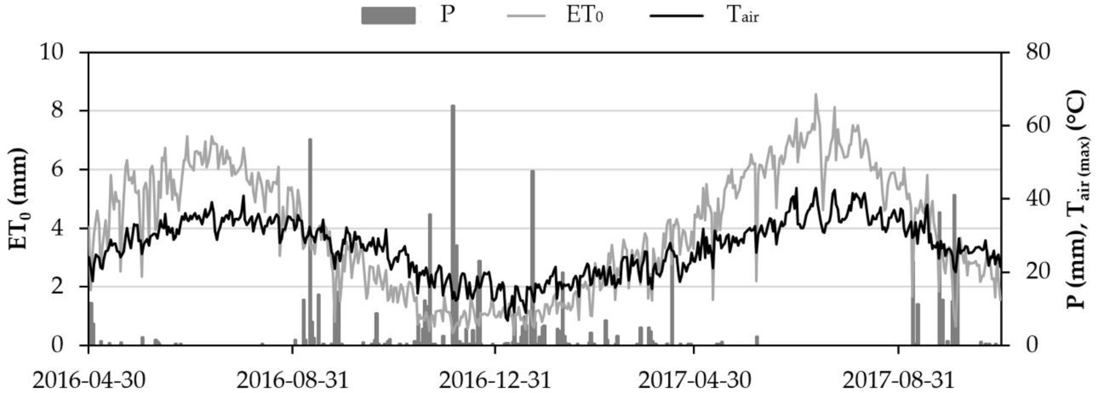
2.4. Ancillary Weather and Soil Data

The ground-based information implemented into the dual Kc FAO-56 model consists of weather observations and soil hydraulic characteristics referring to an experimental orange orchard of 0.7 ha located in southern Italy (Lentini, SR) and managed by Centro di Ricerca Olivicoltura, Frutticoltura e Agrumicoltura of the Italian Council for Agricultural Research and Agricultural Economics Analyses (CREA-OFA, Acireale). The orange orchard has been treated by deficit irrigation strategies, including partial root-zone drying (PRD) and regulated deficit irrigation (RDI), since 2010. The complete description of the experimental site and the irrigation strategies applied are reported in [21,30,31].
Hourly and daily weather data were provided by a meteorological station (37.35°N, 14.91°E, 50 m a.s.l.) located about 2 km from the experimental site and managed by Servizio Informativo Agrometeorologico Siciliano (SIAS; www.sias.regione.sicilia.it).
Weather data (air temperature, Tair, °C; relative humidity, RH, %; precipitation, P, mm; wind speed, u, m s−1; and reference evapotranspiration, ET0, mm), were analyzed in order to initiate/calibrate and implement the SWB model within the dual Kc FAO-56 model.
The temporal evolution of the main weather parameters (ET0, maximum Tair and P) is shown in Figure 3.
The soil hydraulic parameters (i.e., θFC = 0.28 m3 m−3 and θWP = 0.14 m3 m−3) were obtained by laboratory analyses on soil samples collected at the experimental site [21,32] and incorporated into the SWB model within the dual Kc FAO-56 approach.

2.5. Evapotranspiration Validation Using EC

The eddy covariance (EC) method is a direct measurement of a turbulent flux density of a scalar across horizontal wind streamlines [33]. At the experimental site, an EC system is mounted on a tower at 7 m above the surface (about two times the canopy height). The EC system consisted of a three-dimensional sonic anemometer (CSAT3-3D, Campbell Scientific Inc.) and an infrared open-path gas analyzer (Li-7500, Li-cor Biosciences Inc.) to obtain high frequency measurements of the three wind components and the H2O and CO2 concentrations, respectively. The sample frequency for the raw data was 10 Hz (high frequency data) [31]. Low frequency data (30-min) were obtained for: net radiation (Rn, W m−2, net radiometer CNR-1 Kipp & Zonen, located 7 m above the ground) and soil heat flux (G, W m−2), obtained using self-calibrated soil heat flux plates (HFP01SC, Hukseflux) placed in the exposed, half-exposed, and shadowed soil at a depth of about 0.05 m.
High and low frequency data were recorded and stored in a CR1000 logger (Campbell Scientific Inc.).
EC permits to obtain ET rates (ETEC) by the direct measurements of latent heat flux (λET, W m−2) exchanged within the soil-plant-atmosphere continuum, using the following equation:
λ ET EC = λ · σ w q
where λ (J g1) is the latent heat of vaporization and σwq (g m−2 s−1) is the covariance between the vertical wind speed and water vapour density.
EC sensible heat flux (H, W m−2) is computed as:
H = ρ · c p · σ w T
where ρ (g m−3) is the air density, cp (1004 J g−1 K−1) is the air specific heat capacity at constant pressure, and σwT (m s−1 K) is the covariance between the vertical wind speed and air temperature.
The standard EUROFLUX rules [34] were adopted for EC measurements and data processing. Common errors in the measured high frequency data, such as running means for detrending, three angles coordinate rotations, and despiking, were removed during the post processing by quality checks. The stationarity of the surface flux layer and the surface energy balance closure were also evaluated [35]. The surface energy balance closure ratio (CR) is expressed as:
C R = ( H + λ ET ) ( R n G )
and allows for determining how well the turbulent fluxes of heat and water vapor account for the available energy. The ratio, as suggested by [36], was performed only when Rn is greater than 100 W m−2. In this study, the CR was forced according to the procedure proposed by [37], in order to maintain the observed Bowen ratio between H and LE as constant.
Thirty-minute fluxes data were aggregated to a daily scale, and latent heat fluxes, acquired in W m−2, were then transformed to equivalent depth of ET (mm d−1). In this study, ETEC measurements were used as a reference to compare the ET estimates obtained by the original satellite-based dual Kc FAO-56 (ETFAO) approach and the ET estimates (ETERT) obtained by the adjusted model with ERT-derived parameters (few).
Using the ETEC measures (mm d−1) and ET0 by weather station (mm d−1), the crop coefficient using EC (Kc,EC) was estimated, as in the following:
K c , EC = ET EC ET 0 .

2.6. Water Stress Coefficient Determination

The above described dual Kc FAO 56 approaches (both the original and ERT-adjusted) compute ET under standard conditions (i.e., water stress coefficient, Ks, equal to 1), whereas ET measured using the EC technique (ETEC) incorporates soil water stress condition (ETEC = Ks Kc,EC ET0; Kc,EC being the hypothetical Kc value that will be measured by EC in the absence of water stress). Thus, assuming that Kc,ERT is equal to Kc,EC, Ks can be empirically derived as:
K s = ET EC ET ERT = K s · K C , EC · ET 0 K cERT · ET 0 .

3. Results

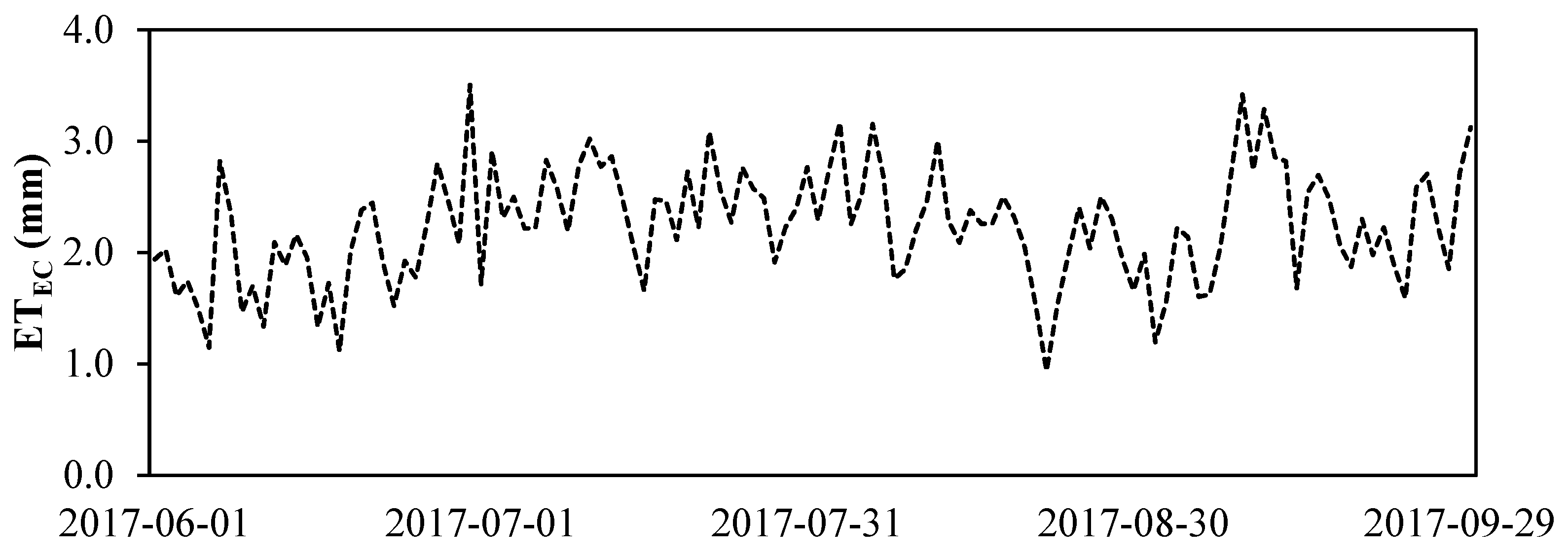
3.1. Evapotranspiration Rates using EC

The temporal evolution of daily scale ETEC rates within the reference period (June–September 2017) is shown in Figure 4. ETEC rates ranged between 0.94 and 3.50 mm day−1, with a mean value of 2.24 mm d−1. Prior to the CR adjustment, the slope of the regression forced through the origin of the CR was around 0.82, with a determination coefficient (R2) of about 0.90.

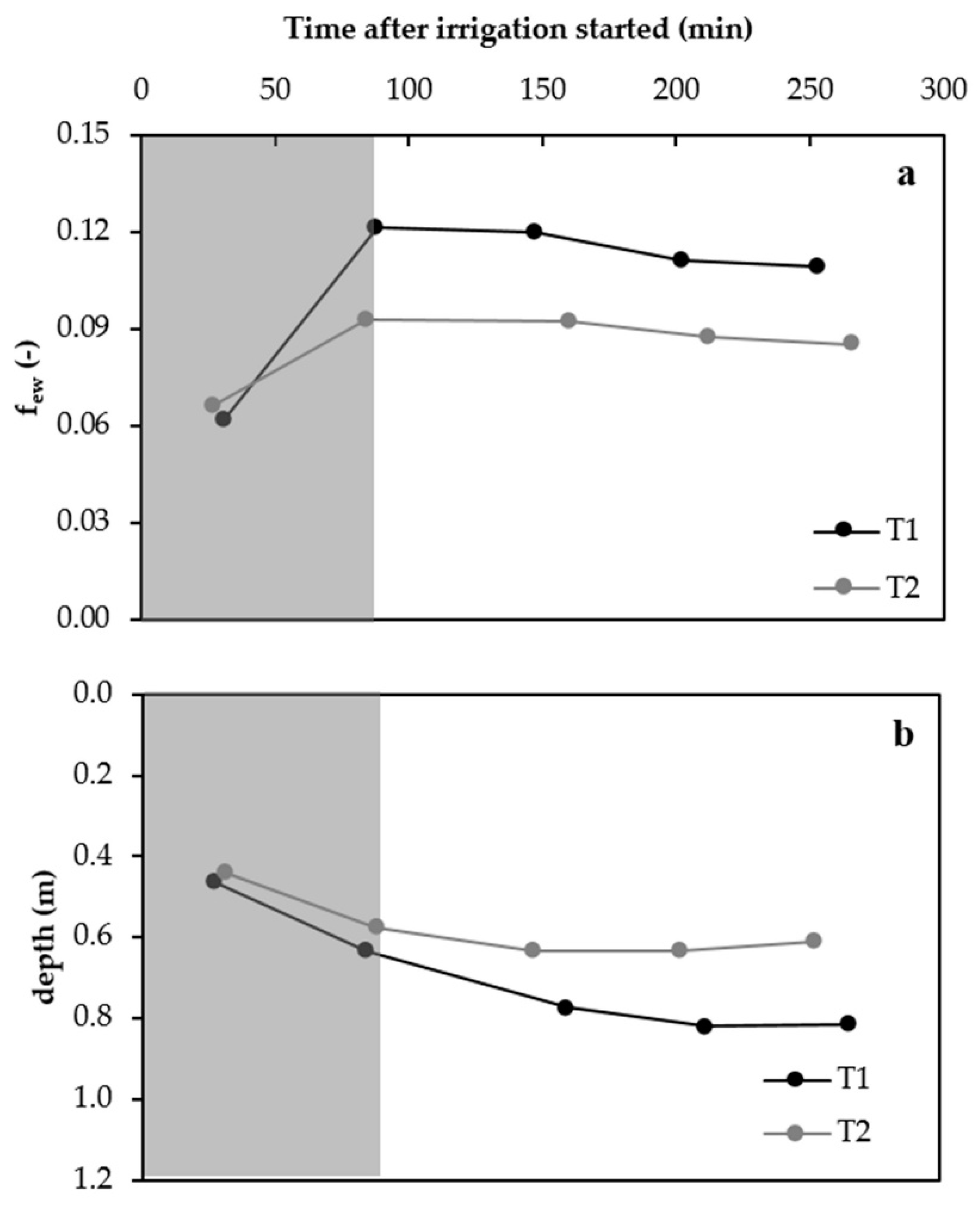
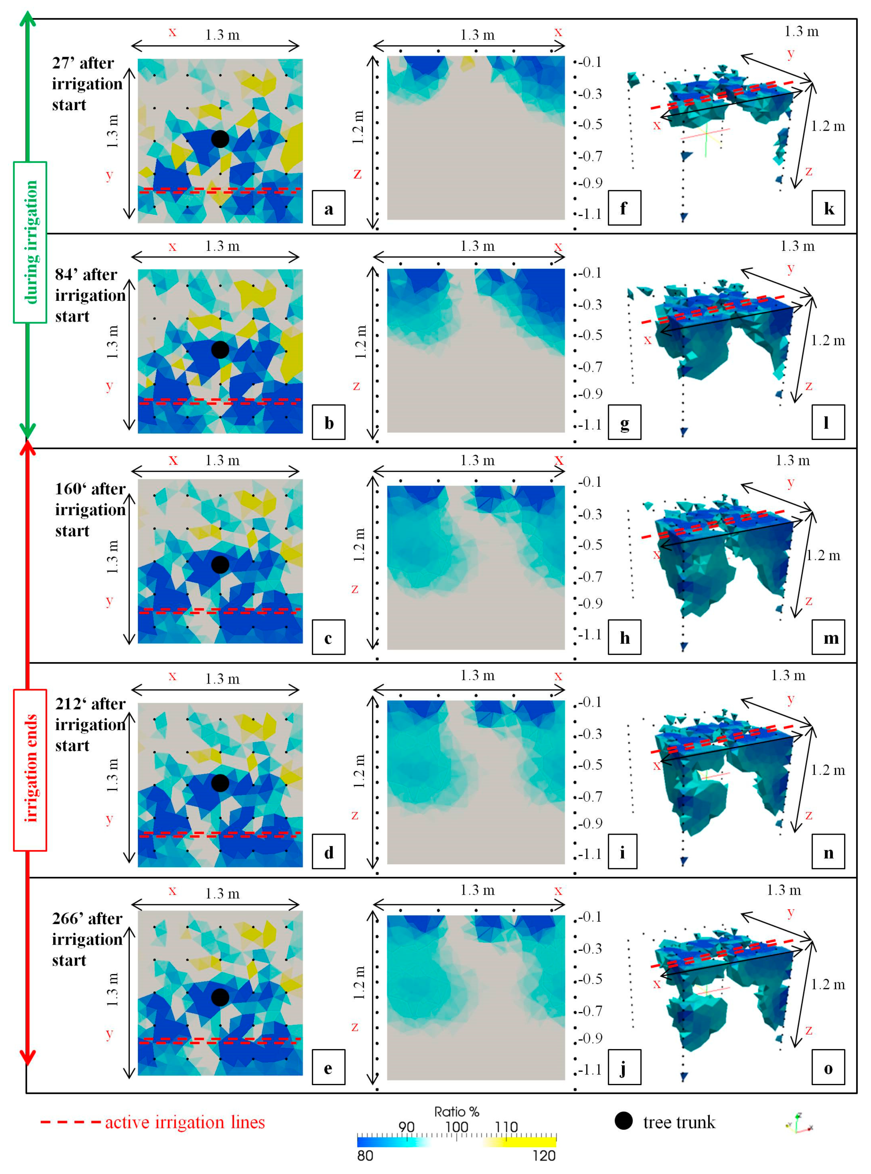
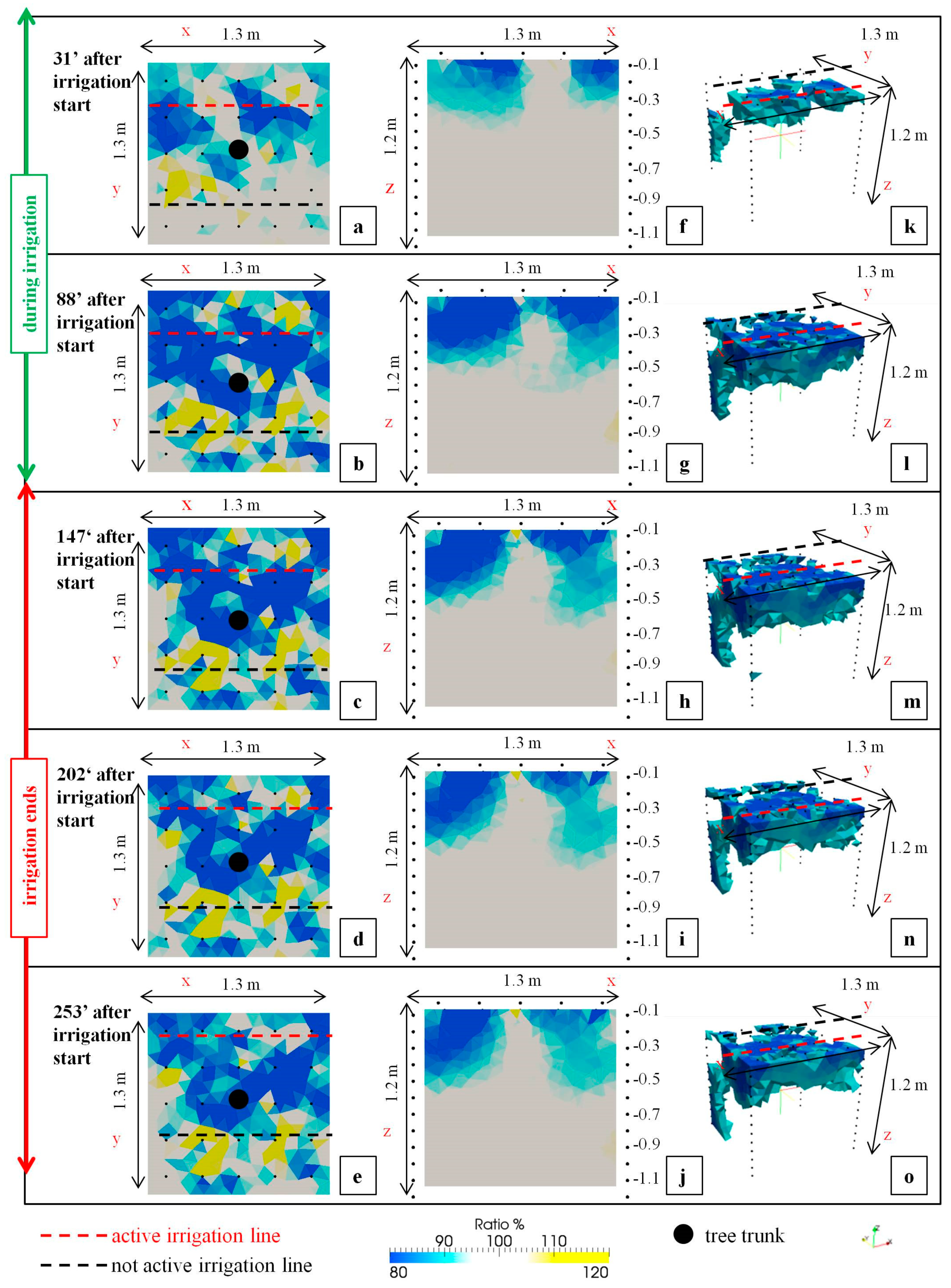
3.2. Soil Wetting Distribution Patterns Using ERT

Figure 5 and Figure 6 show the changes in ER ratio (at the surface: a–e; transects under the irrigation pipeline: f–j; and 3-D volumes: k–o) observed during and after the irrigation phase (Table 1), compared to the initial condition (no irrigation), in T1 and T2. A value of 100% indicates no change in ER terms with respect to the initial condition; values higher and lower than 100% indicate increases (drying patterns) and decreases of ER (wetting patterns), respectively. Both in T1 and T2, the main phenomenon occurring within the explored ERT volume was an ER ratio decreasing (soil wetting patterns), even if localized areas (less than 1% of the overall explored volume) were characterized by ER increasing (drying patterns) with respect to the initial condition (Table 1).
Figure 2a shows the evolution of the exposed wetted area (few) during and after the irrigation phase in T1 and T2. The mean few value obtained from both T1 and T2 was 0.1. This value was used for running the SWB model within the ERT-adjusted dual Kc FAO-56 approach.
At the surface level, the main ER decreasing patterns are localized close to the active irrigation pipeline, both T1 and T2, during the irrigation phase (Figure 5a,b, Figure 6a,b and Figure 2a). Nevertheless, once the irrigation phase finished (after about 88 min from the irrigation start, Table 1), patterns in ER decreasing are always observed (time 03, Figure 5c, Figure 6c and Figure 2a). At times 04–05 (Table 1, Figure 2a) the same patterns became quite steady showing a slight increase.
Figure 2b shows the evolution of the infiltration front depth (m) during and after the irrigation phase in T1 and T2. Analyzing the ER changes from the top soil to the bottom-layer (Figure 5f–j and Figure 6f–j), two phases were identified. During the irrigation phase, an increase of the infiltration front depth was observed both in T1 and T2, but with different magnitudes. In fact, in T1, where the full irrigation is applied, the wetting patterns distribution reached greater depths than T2 (supplied at 50% in respect to T1 irrigation rate) with a maximum of 0.8 and 0.6 m, respectively. After the irrigation end, the infiltration front remained almost constant or even evidenced a slight depth reduction (Figure 5f–j, Figure 6f–j and Figure 2b).
At 3-D level (Figure 5k–o and Figure 6k–o), during the irrigation phase (times 01 and 02 in Table 1; and Figure 5k,l and Figure 6k,l), a marked decrease in ER ratio (values equal to or less than 90%) was observed. ER reductions ranged from 5% to 16% on average of the overall explored volume in T1 and T2, due to progression of the irrigation front in correspondence with the active irrigation pipelines (2 drip irrigation emitters on the surface of T1 and T2 within the ERT explored volume). After the irrigation phase (time 03 in Table 1; and Figure 5m and Figure 6m), the wetting volumes became quite stable, around 16% of the total volume, followed by a slight decrease until 12–13% (times 04 and 05 in Table 1; and Figure 5n–o and Figure 6n–o).

3.3. Satellite dual Kc Approach

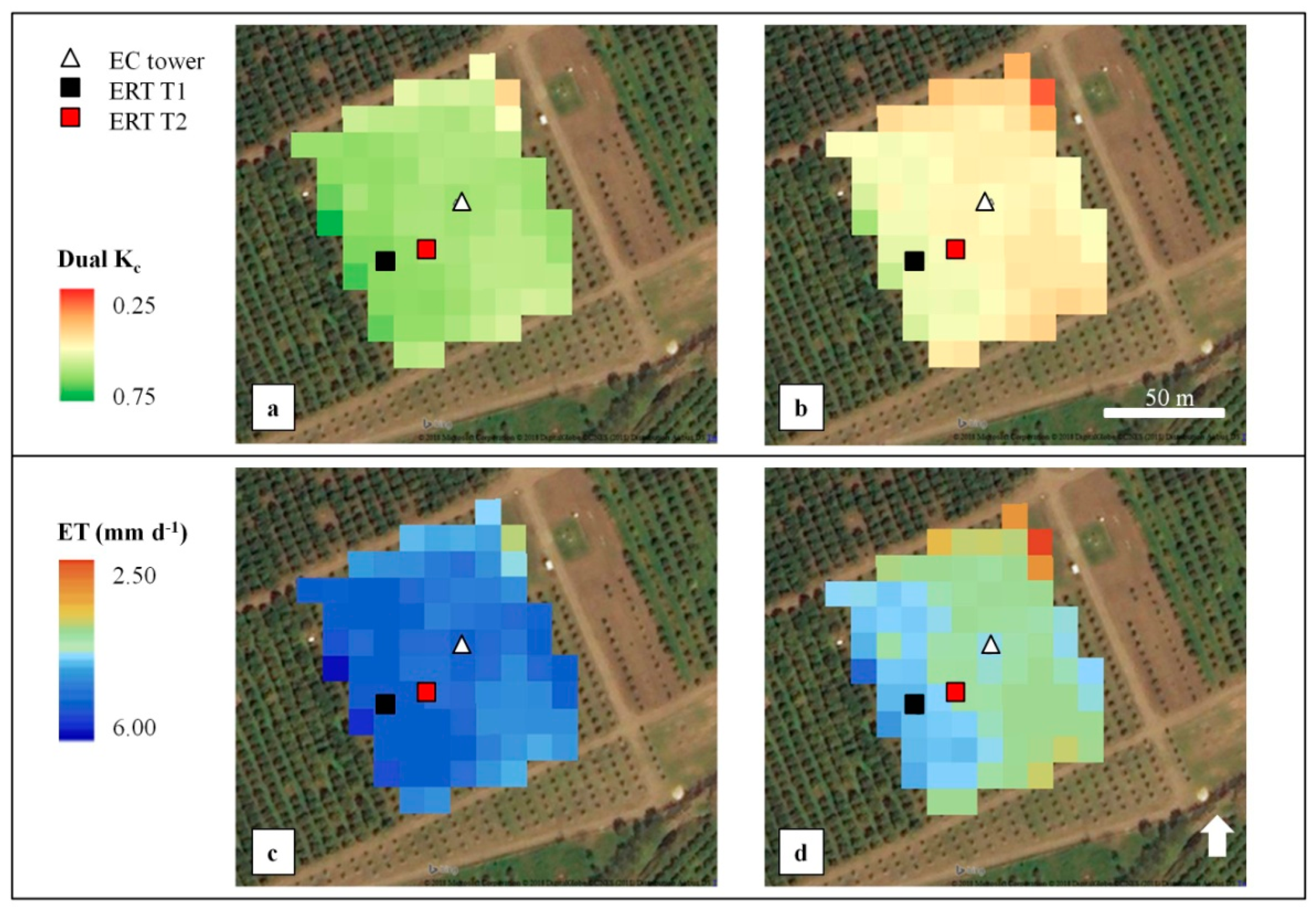
3.3.1. Maps of original and ERT-adjusted dual Kc FAO-56

Figure 7 shows an example of spatially distributed estimates of dual Kc (Kc,FAO and Kc,ERT; a,b) and ET (ETFAO and ETERT; c,d) obtained for the study area by the original and ERT-adjusted dual Kc FAO-56 approach for DOY 193 (under ET0 conditions of 8.56 mm day−1). The dual Kc values derived from FAO-56 and ERT-adjusted approaches were 0.69 and 0.59, respectively, resulting in ET values of 5.91 (ETFAO) and 5.06 mm (ETERT).

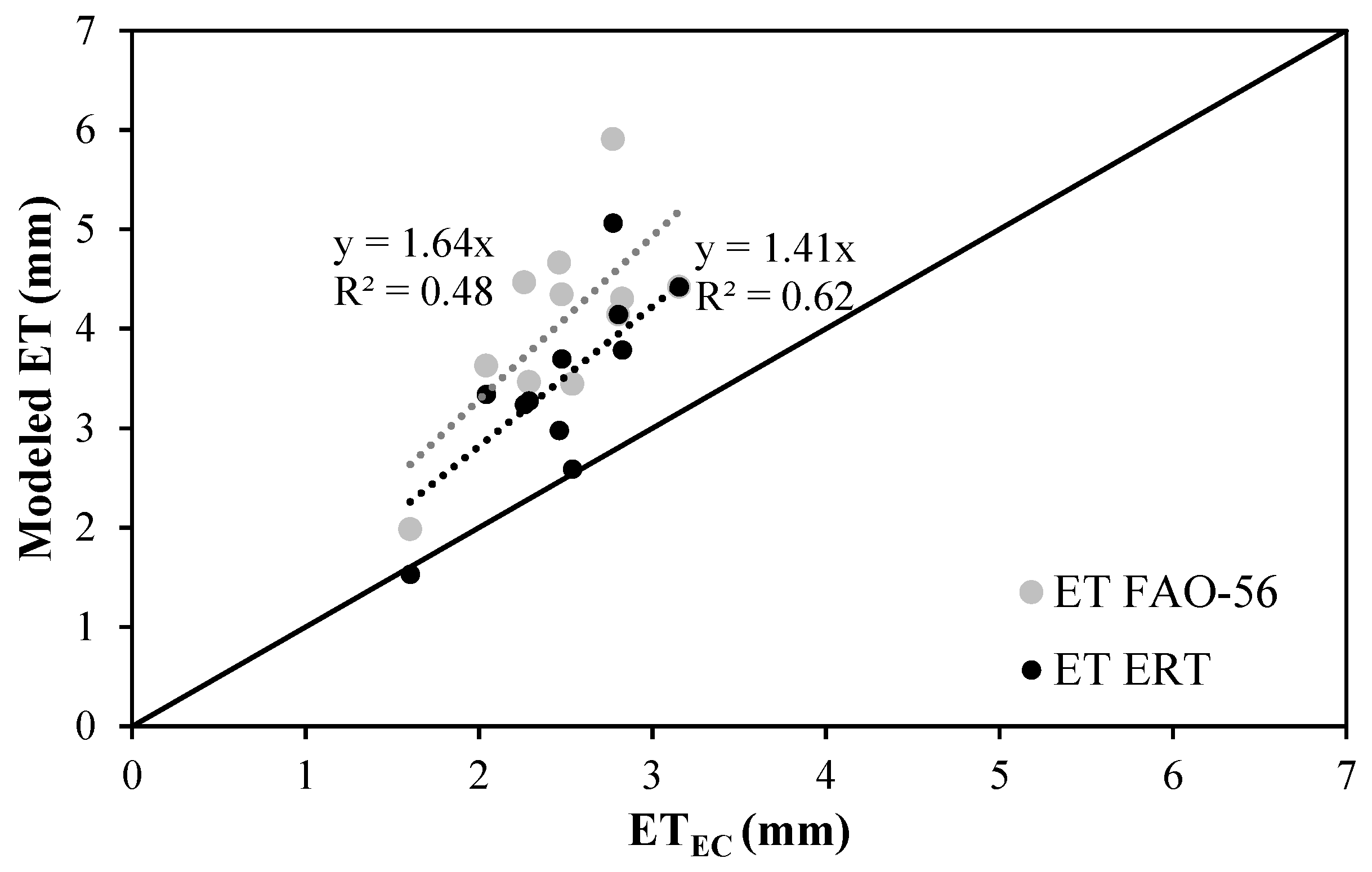
3.3.2. ET Comparison: Original and ERT-Adjusted Dual Kc FAO-56 vs EC

Figure 8 shows the scatterplot between the daily measured ETEC, the original (ETFAO), and the ERT-adjusted (ETERT) dual Kc FAO-56 approaches satellite ET estimates.
Daily modelled ET values (ETFAO and ETERT, with average values of 4.07 and 3.46 mm, respectively) resulted in an average 64% and 40% greater than the measured ETEC fluxes (average value of 2.47 mm), with root mean square errors (RMSE) of 1.74 and 1.17 mm day−1 and coefficients of determination (R2) of 0.48 and 0.62, respectively. The slope terms were 1.64 and 1.41 for ETFAO and ETERT respectively, reflecting that ET discrepancies with respect to ETEC were greater for high ET values. The average T component was 3.19 mm for both original and ERT-adjusted dual Kc FAO-56 approaches, whereas E term was 0.88 mm and 0.27 mm, respectively.

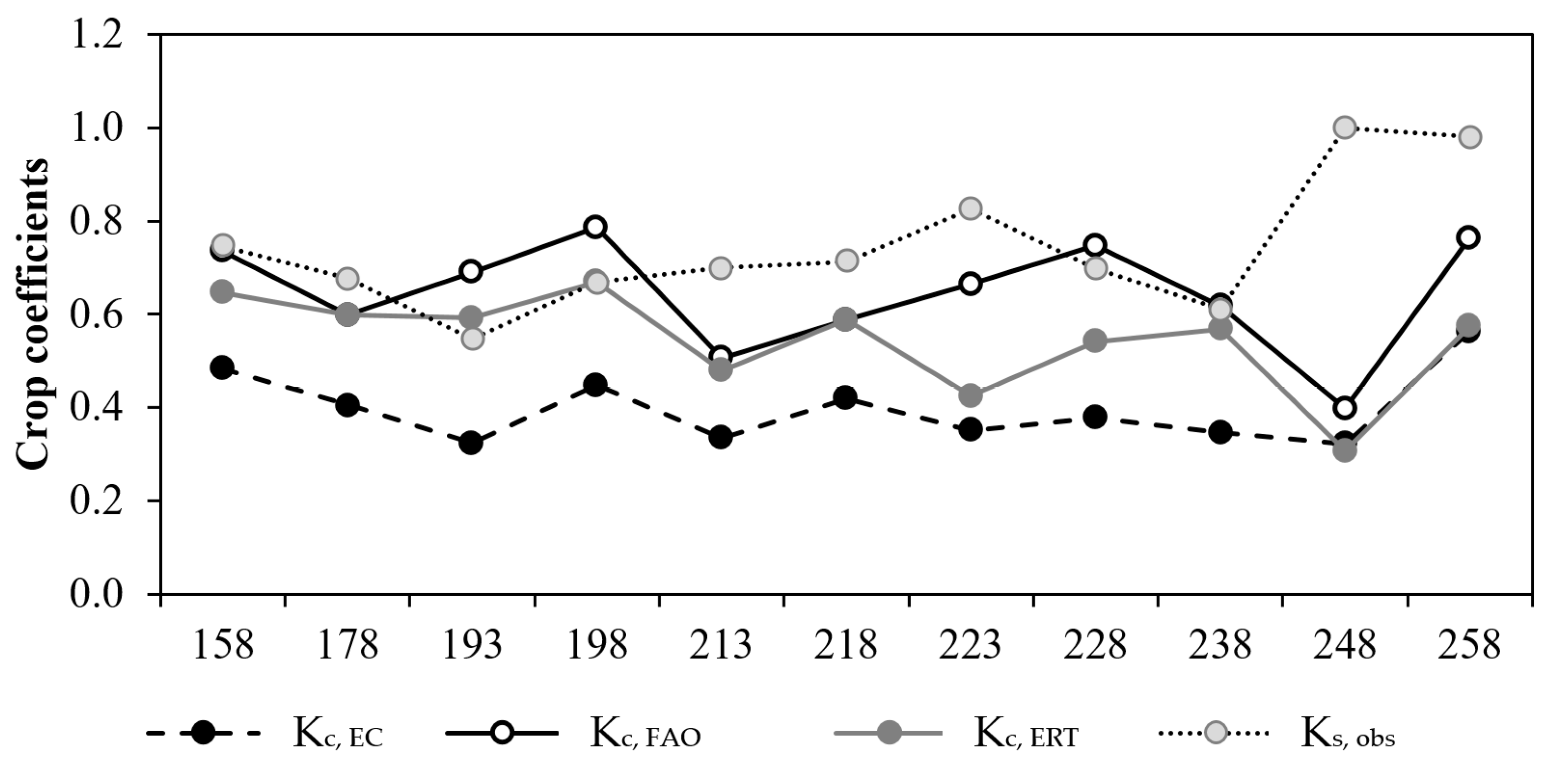
3.3.3. Crop Coefficients Comparison and Ks Estimation

Figure 9 shows the crop coefficients (Kcb + Ke) obtained from EC (Kc,EC) and from the original (Kc,FAO) and ERT-adjusted (Kc,ERT) dual Kc FAO-56 approaches. Within the reference period (June–September 2017), the observed Kc using EC (Kc,EC) was 0.40 ± 0.08. For the same period, Kc,FAO and Kc,ERT resulted in 0.64 ± 0.12 and 0.54 ± 0.11, respectively.
Temporal evolution of water stress coefficient (Ks) obtained as Equation (13) is reported in Figure 9. Ks values ranged from 0.55 to 1.00 with an average of 0.74.

4. Discussion

The need of accurate ET estimates from remote sensing data calls for simplified methods to be applied at a wide range of spatial resolutions [38]. The lack of useful applications may be overcome by combining different multi-platforms data [39] or by using modelling [40,41], as in this study, by combining remote sensing data with geophysical information.
The most remarkable features of the ERT time-lapse inversions in Figure 5 and Figure 6 are the decreasing of ER ratio (wetting patterns) that seem to change substantially over time. As irrigation occurs in a very contained portion of the area monitored by ERT, it is not surprising that ER tends to decline largely in correspondence to drippers activity, creating consistent soil wetting patterns that extend from the surface to the bottom of the monitored soil volume (1.2 m depth) during irrigation and tends to become steady or decrease at the end of the irrigation phase (Figure 5 and Figure 6). The different magnitude of these changes among treatments at localized depths is explained by the different irrigation rates applied in T1 (full irrigation) and T2 (deficit irrigation under PRD). Drying patterns (increasing of ER ratio) observed close to the surface can be attributed to direct evaporation from the top soil or root-water-uptake processes [22] or to inversion artefacts [42]. Due to the complexity of the hydrological processes that act within the soil-root system, an integration of hydrological and geophysical modelling might improve the analysis of recorded ER patterns [43].
The few information retrieved using ERT were herein included in the adjusted satellite dual Kc FAO-56 approach. The obtained results showed that ERT improved ET estimates (and E), with respect to the estimates obtained by the original dual Kc FAO-56 approach, when compared with the site-specific ETEC rates measured at the experimental site by EC. In fact, the comparison between Kc,FAO and Kc,ERT reveals that Kc,ERT was always lower than Kc,FAO, this discrepancy being due to the more accurate estimation of few performed in the ERT-adjusted approach. Consequently, with the ERT-adjusted approach, the E term, and therefore ET, was considerably reduced (15%) when compared with the original dual Kc FAO-56 approach [14]. Nevertheless, ET obtained from both approaches, even considering the ERT-adjustment, remained substantially higher than ET measured in EC (64% and 40%, respectively). Such overestimations could be due to the assumption taken in this study of considering few constant during the day, since it is well known that few progressively diminish after an irrigation event. Additionally, the presence of different irrigation treatments within the footprint of the EC tower may introduce some uncertainties in the results obtained. In addition, the spatial resolution of Sentinel does not allow the separation of regions irrigated differentially. Therefore, this limitation could be solved by using high spatial resolution images, such as those acquired by unmanned aerial vehicles, which would allow the few of each irrigation treatment to be considered separately instead of averaging both of them, as done for mixed pixels. Similar to the results obtained in this study, several authors have found ET overestimation ranging from 12% to 42% when comparing ET from the FAO 56 approach with ET provided by EC in heterogeneous orchards under drip irrigation [44,45] indicating that the overestimation was even worse when examining only the irrigated period [46]. These authors pointed out that the values of Kcb suggested by [14,45,46] and the high soil evaporation predicted following the FAO-56 approach [45,46] as the main reasons for these overestimations. In general, the magnitude of such overestimations was lower than the one obtained in this study probably due to the water stress expected in our experiment as consequence of the deficit irrigation conditions applied at the experimental site. Deficit irrigation strategy played a strategic role in altering the normal ratio between the energy balance surface fluxes, determining a fairly high sensible heat flux and an ET reduction or underestimation due to the imposed water stress conditions [31]. This behavior was poorly captured by the original and the ERT-adjusted Kc FAO-56 approaches, whereas it was taken into account in the ETEC value obtained using the EC technique, as indicated by the calculated Ks (≈0.74).
Despite the good results obtained using 3-D ERT for helping to estimate ET, future developments of this technique should attempt for speed operational applications (e.g., the need for real time data). Additionally, future research should address the mid–long term temporal evolution of few to better characterize changes in soil water conditions and subsequently evaporation, in order to incorporate dynamic few values into the approach instead of using a constant one. At this stage, ERT may be considered a useful tool for precision irrigation strategies, in particular for identifying the soil wetting patterns distribution and also allowing a better characterization of the wet bulb, which may therefore improve the efficiency of irrigation [21]. Currently, the scope of ERT is limited to scientific research or as a validation method for calibrating other methods that can be more easily incorporated into the daily activities of farmers and technicians. In the future, more commercially oriented applications of ERT technologies could be derived in order to facilitate the implementation of this technique for agriculture water management applications.

5. Conclusions

The main conclusions to be drawn from this study can be summarized as follows:
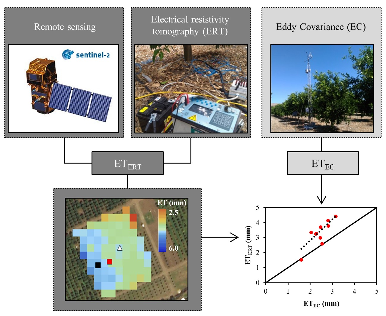
  • Spatially distributed ET rates can be obtained by incorporating VIs computed using remote sensing technologies into the dual Kc FAO-56 approach.
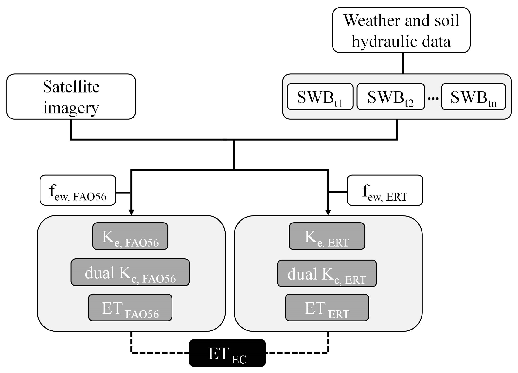
  • The integration of 3-D ERT methodology into the dual Kc FAO-56 approach considerably reduced errors in ET estimates. This technology allowed the tracking of the wetting distribution patterns, helping to accurately estimate few and therefore the water evaporated from the soil surface.
  • The dual Kc FAO-56 approach determines ET under standard conditions where no limitations are placed on crop growth or ET, whereas EC measures ET even for non-standard conditions (e.g., under soil water stress conditions). From the comparison between the ET measured from the EC tower and the ET estimated from the ERT-adjusted dual Kc FAO-56 approach, the Ks term can be experimentally derived.

Author Contributions

The authors contributed with equal effort to the realization of the study.

Funding

The authors thank the EU, the Italian Ministry of Education, Universities and Research, and the Spanish Agencia Estatal de Investigación for funding, as part of the collaborative international consortium IRIDA (‘‘Innovative remote and ground sensors, data and tools into a decision support system for agriculture water management”), financed under the ERA-NET Cofund WaterWorks 2014. This ERA-NET is an integral part of the 2015 Joint Activities developed by the Water Challenges for a Changing World Joint Programme Initiative (Water JPI). The authors also acknowledge support from the ERANET-MED project WASA (‘‘Water Saving in Agriculture: Technological developments for the sustainable management of limited water resources in the Mediterranean area”).

Acknowledgments

The authors wish to thank Servizio Informativo Agrometeorologico Siciliano (SIAS) for weather data and the personnel of Centro di Ricerca Olivicoltura, Frutticoltura e Agrumicoltura of the Italian Council for Agricultural Research and Agricultural Economics Analyses (CREA-OFA, Acireale) for their hospitality at the experimental site.

Conflicts of Interest

The authors declare no conflicts of interest. The funders had no role in the design of the study; in the collection, analyses, or interpretation of data; in the writing of the manuscript, and in the decision to publish the results.

References

  1. French, R.J.; Schultz, J.E. Water use efficiency of wheat in a Mediterranean type environment. I. The relation between yield, water use and climate. Aust. J. Agric. Res. 1984, 35, 743–764. [Google Scholar] [CrossRef]
  2. French, R.J.; Schultz, J.E. Water use efficiency of wheat in a mediterranean-type environment. II. Some limitations to efficiency. Aust. J. Agric. Res. 1984, 35, 765–775. [Google Scholar] [CrossRef]
  3. Capra, A.; Consoli, S.; Russo, A.; Scicolone, B. Integrated agro-economic approach to deficit irrigation on lettuce crops in Sicily (Italy). J. Irrig. Drain. Eng. 2008, 134, 437–445. [Google Scholar] [CrossRef]
  4. Consoli, S.; Papa, R. Corrected surface energy balance to measure and model the evapotranspiration of irrigated orange orchards in semi-arid Mediterranean conditions. Irrig. Sci. 2013, 31, 1159–1171. [Google Scholar] [CrossRef]
  5. Zhao, P.; Kang, S.; Li, S.; Ding, R.; Tong, L.; Du, T. Seasonal variations in vineyard ET partitioning and dual crop coefficients correlate with canopy development and surface soil moisture. Agric. Water Manag. 2018, 197, 19–33. [Google Scholar] [CrossRef]
  6. Yau, S.K.; Nimah, M.; Farran, M. Early sowing and irrigation to increase barley yields and water use efficiency in Mediterranean conditions. Agric. Water Manag. 2011, 98, 1776–1781. [Google Scholar] [CrossRef]
  7. Yan, A.; Gao, C.; Ren, Y.; Zong, R.; Ma, Y.; Li, Q. Effects of pre-sowing irrigation and straw mulching on the grain yield and water use efficiency of summer maize in the North China Plain. Agric. Water Manag. 2017, 186, 21–28. [Google Scholar] [CrossRef]
  8. Eastham, J.; Gregory, P.J.; Williamson, D.R.; Watson, G.D. The influence of early seeding of wheat and lupin crops on evapotranspiration and evaporation from the soil surface in a Mediterranean climate. Agric. Water Manag. 1999, 42, 205–218. [Google Scholar] [CrossRef]
  9. Liu, C.M.; Zhang, X.Y.; Zhang, Y.Q. Determination of daily evaporation and evapotranspiration of winter wheat and maize by large-scale weighing lysimeter and micro-lysimeter. Agric. For. Meteorol. 2002, 111, 109–120. [Google Scholar] [CrossRef]
  10. Photiades, A.; Hadjichristodoulou, A. Sowing date, sowing depth, seed rate and row spacing of wheat and barley under dryland conditions. Field Crops Res. 1984, 9, 151–162. [Google Scholar] [CrossRef]
  11. Lascano, R.J.; Baumhardt, R.L.; Hicks, S.K.; Heilman, J.L. Soil and plant water evaporation from strip-tillage control, measurement and simulation. Agron. J. 1994, 86, 987–994. [Google Scholar] [CrossRef]
  12. Stagnari, F.; Galieni, A.; Speca, S.; Cafiero, G.; Pisante, M. Effects of straw mulch on growth and yield of durum wheat during transition to Conservation Agriculture in Mediterranean environment. Field Crops Res. 2014, 167, 51–63. [Google Scholar] [CrossRef]
  13. Prosdocimi, M.; Jordan, A.; Tarolli, P.; Keesstra, S.; Novara, A.; Cerda, A. The immediate effectiveness of barley straw mulch in reducing soil erodibility and surface runoff generation in Mediterranean vineyards. Sci. Total Environ. 2016, 547, 323–330. [Google Scholar] [CrossRef] [PubMed] [Green Version]
  14. Allen, R.G.; Pereira, L.S.; Raes, D.; Smith, M. Crop Evapotranspiration-Guidelines for Computing Crop Water Requirements-FAO Irrigation and Drainage Paper 56; FAO: Rome, Italy, 1998; Volume 300, p. D05109. [Google Scholar]
  15. González-Dugo, M.P.; Neale, C.M.U.; Mateos, L.; Kustas, W.P.; Prueger, J.H.; Anderson, M.C.; Li, F. A comparison of operational remote sensing-based models forestimating crop evapotranspiration. Agric. For. Meteorol. 2009, 149, 1843–1853. [Google Scholar] [CrossRef]
  16. Subbaiah, R. A review of models for predicting soil water dynamics during trickle irrigation. Irrig. Sci. 2013, 31, 225–258. [Google Scholar] [CrossRef]
  17. Jarvis, N.; Koestel, J.; Larsbo, M. Understanding preferential flow in the vadose zone: Recent advances and future prospects. Vadose Zone J. 2016, 15, 15. [Google Scholar] [CrossRef]
  18. Hardie, M.; Ridges, J.; Swarts, N.; Close, D. Drip irrigation wetting patterns and nitrate distribution: Comparison between electrical resistivity (ERI), dye tracer, and 2D soil–water modelling approaches. Irrig. Sci. 2018, 36, 97–110. [Google Scholar] [CrossRef]
  19. Cassiani, G.; Boaga, J.; Vanella, D.; Perri, M.T.; Consoli, S. Monitoring and modelling of soil–plant interactions: The joint use of ERT, sap flow and eddy covariance data to characterize the volume of an orange tree root zone. Hydrol. Earth Syst. Sci. 2015, 19, 2213–2225. [Google Scholar] [CrossRef]
  20. Cassiani, G.; Boaga, J.; Rossi, M.; Putti, M.; Fadda, G.; Majone, B.; Bellin, A. Soil–plant interaction monitoring: Small scale example of an apple orchard in Trentino, North-eastern Italy. Sci. Total Environ. 2016, 543, 851–861. [Google Scholar] [CrossRef]
  21. Consoli, S.; Stagno, F.; Vanella, D.; Boaga, J.; Cassiani, G.; Roccuzzo, G. Partial root-zone drying irrigation in orange orchards: Effects on water use and crop production characteristics. Eur. J. Agron. 2017, 82, 190–202. [Google Scholar] [CrossRef]
  22. Vanella, D.; Cassiani, G.; Busato, L.; Boaga, J.; Barbagallo, S.; Binley, A.; Consoli, S. Use of small scale electrical resistivity tomography to identify soil-root interactions during deficit irrigation. J. Hydrol. 2018, 556, 310–324. [Google Scholar] [CrossRef]
  23. Binley, A.M.; Kemna, A. DC resistivity and induced polarization methods. In Hydrogeophysics; Rubin, Y., Hubbard, S.S., Eds.; Springer: Dordrecht, The Netherlands, 2005; Volume 50, pp. 129–156. [Google Scholar] [CrossRef]
  24. Binley, A. Tools and techniques: DC electrical methods. In Treatise on Geophysics, 2nd ed.; Schubert, G., Ed.; Elsevier: Amsterdam, The Netherlands, 2015; Volume 11, pp. 233–259. [Google Scholar] [CrossRef]
  25. Consoli, S.; Vanella, D. Comparisons of satellite-based models for estimating evapotranspiration fluxes. J. Hydrol. 2014, 513, 475–489. [Google Scholar] [CrossRef]
  26. Consoli, S.; Vanella, D. Mapping crop evapotranspiration by integrating vegetation indices into a soil water balance model. Agric. Water Manag. 2014, 143, 71–81. [Google Scholar] [CrossRef]
  27. Huete, A.R. A soil-adjusted vegetation index (SAVI). Remote Sens. Environ. 1988, 25, 295–309. [Google Scholar] [CrossRef]
  28. Gutman, G.; Ignatov, A. The derivation of the green vegetation fraction from NOAA/AVHRR data for use in numerical weather prediction models. Int. J. Remote Sens. 1998, 19, 1533–1543. [Google Scholar] [CrossRef]
  29. Rouse, J.W.; Haas, R.H.; Schell, J.A.; Deering, D.W.; Harlan, J.C. Monitoringthe Vernal Advancement and Retrogradation of Natural Vegetation; Type III, Final Report; NASA/GSFC: Greenbelt, MD, USA, 1974; pp. 1–371.
  30. Consoli, S.; Stagno, F.; Roccuzzo, G.; Cirelli, G.; Intrigliolo, F. Sustainable management of limited water resources in a young orange orchard. Agric. Water Manag. 2014, 132, 60–68. [Google Scholar] [CrossRef]
  31. Vanella, D.; Consoli, S. Eddy Covariance fluxes versus satellite-based modelisation in a deficit irrigated orchard. Ital. J. Agrometeorol. 2018, 2, 41–52. [Google Scholar] [CrossRef]
  32. Aiello, R.; Bagarello, V.; Barbagallo, S.; Consoli, S.; Di Prima, S.; Giordano, G.; Iovino, M. An assessment of the Beerkan method for determining the hydraulic properties of a sandy loam soil. Geoderma 2014, 235, 300–307. [Google Scholar] [CrossRef]
  33. Baldocchi, D.D. Assessing the eddy covariance technique for evaluating carbon dioxide exchange rates of ecosystems: Past, present and future. Glob. Chang. Biol. 2003, 9, 479–492. [Google Scholar] [CrossRef]
  34. Aubinet, M.; Grelle, A.; Ibrom, A.; Rannik, U.; Moncrieff, J.; Foken, T.; Kowalski, A.S.; Martin, P.H.; Berbigier, P.; Bernhofer, C.; et al. Estimates of the annual net carbon and water exchange of European forests: The EUROFLUX methodology. Adv. Ecol. Res. 2000, 30, 113–175. [Google Scholar]
  35. Kaimal, J.C.; Finnigan, J.J. Atmospheric Boundary-Layer Flows: Their Structure and Measurement; Oxford University Press: Oxford, UK, 1994; 289p. [Google Scholar]
  36. Prueger, J.H.; Hatfield, J.L.; Kustas, W.P.; Hipps, L.E.; MacPherson, J.I.; Parkin, T.B. Tower and aircraft eddy covariance measurements of water vapor, energy and carbon dioxide fluxes during SMACEX. J. Hydrometeorol. 2005, 6, 954–960. [Google Scholar] [CrossRef]
  37. Twine, T.E.; Kustas, W.P.; Norman, J.M.; Cook, D.R.; Houser, P.; Meyers, T.P.; Prueger, J.H.; Starksh, P.J.; Wesely, M.L. Correcting eddy-covariance flux underestimates over a grassland. Agric. For. Meteorol. 2000, 103, 279–300. [Google Scholar] [CrossRef] [Green Version]
  38. Wang, K.; Liang, S. An improved method for estimating global evapotranspiration based on satellite determination of surface net radiation, vegetation index, temperature, and soil moisture. J. Hydrometeorol. 2008, 9, 712–727. [Google Scholar] [CrossRef]
  39. Knipper, K.; Hogue, T.; Scott, R.; Franz, K. Evapotranspiration estimates derived using multi-platform remote sensing in a semiarid region. Remote Sens. 2017, 9, 184. [Google Scholar] [CrossRef]
  40. Sun, G.; Alstad, K.; Chen, J.; Chen, S.; Ford, C.R.; Lin, G.; Liu, C.; Lu, N.; McNulty, S.G.; Miao, H.; et al. A general predictive model for estimating monthly ecosystem evapotranspiration. Ecohydrology 2011, 4, 245–255. [Google Scholar] [CrossRef]
  41. Consoli, S.; Licciardello, F.; Vanella, D.; Pasotti, L.; Villani, G.; Tomei, F. Testing the water balance model criteria using TDR measurements, micrometeorological data and satellite-based information. Agric. Water Manag. 2016, 170, 68–80. [Google Scholar] [CrossRef]
  42. Kim, J.H.; Yi, M.J.; Park, S.G.; Kim, J.G. 4-D inversion of DC resistivity monitoring data acquired over a dynamically changing earth model. J. Appl. Geophys. 2009, 68, 522–532. [Google Scholar] [CrossRef]
  43. Busato, L.; Boaga, J.; Perri, M.T.; Majone, B.; Bellin, A.; Cassiani, G. Hydrogeophysical characterization and monitoring of the hyporheic and riparian zones: The Vermigliana Creek case study. Sci. Total Environ. 2018, 648, 1105–1120. [Google Scholar] [CrossRef]
  44. Paço, T.A.; Ferreira, M.I.; Conceição, N. Peach orchard evapotranspiration in a sandy soil: Comparison between eddy covariance measurements and estimates by the FAO 56 approach. Agric. Water Manag. 2006, 85, 305–313. [Google Scholar] [CrossRef]
  45. Er-Raki, S.; Chehbouni, A.; Guemouria, J.; Ezzahar, J.; Khabba, S.; Boulet, G.; Hanich, L. Citrus orchard evapotranspiration: Comparison between eddy covariance measurements and the FAO-56 approach estimates. Plant Biosyst. 2009, 143, 201–208. [Google Scholar] [CrossRef] [Green Version]
  46. Maestre-Valero, J.F.; Testi, L.; Jiménez-Bello, M.A.; Castel, J.R.; Intrigliolo, D.S. Evapotranspiration and carbon exchange in a citrus orchard using eddy covariance. Irrig. Sci. 2017, 35, 397–408. [Google Scholar] [CrossRef]
Figure 1. Scheme of the methodology applied in this study.
Remotesensing 11 00373 g001
Figure 2. Evolution of the exposed wetted area (few) (a) and evolution of the infiltration front depth (m) in T1 and T2 during and after an irrigation phase (b). Time is expressed in minutes after the irrigation start. The grey area represents the irrigation phase period.
Remotesensing 11 00373 g002
Figure 3. Temporal evolution of weather parameters used to implement the soil water balance (SWB) model within the dual Kc FAO-56 approach. Values refer to the reference period (April 2016–October 2017). P is the precipitation (mm); ET0 is the reference evapotranspiration (mm); and Tair is the air temperature (°C).
Remotesensing 11 00373 g003
Figure 4. Temporal evolution of daily evapotranspiration measurements (ETEC) rates using eddy covariance (EC).
Remotesensing 11 00373 g004
Figure 5. Time-lapse electrical resistivity (ER) ratio imagery (at the surface: ae; transects under the irrigation pipeline: fj; and 3-D volumes: ko) for T1 with respect to the initial condition (no irrigation).
Remotesensing 11 00373 g005
Figure 6. Time-lapse electrical resistivity (ER) ratio imagery (at the surface: ae; transects under the irrigation line: fj; and 3-D volumes: ko) for T2 with respect to the initial condition (no irrigation).
Remotesensing 11 00373 g006
Figure 7. Dual crop coefficient (Kc,FAO and Kc,ERT; a,b) and ET (ETFAO and ETERT; c,d) estimates obtained by the original and ERT-adjusted dual Kc FAO-56 approach for DOY 193 (under ET0 conditions of 8.56 mm day−1).
Remotesensing 11 00373 g007
Figure 8. Comparison between modelled ETFAO and ETERT versus measured ETEC. The black solid line represents the 1:1 relationship.
Remotesensing 11 00373 g008
Figure 9. Kc from EC (Kc,EC) and from the original (Kc,FAO) and ERT-adjusted dual Kc FAO-56 approach (Kc,ERT), and Ks derived from ETEC and ETERT ratio.
Remotesensing 11 00373 g009
Table 1. Three-dimensional (3-D) electrical resistivity tomography (ERT) data collection time (local time).
T1T2
Time IdStateStarting TimeEnding TimeStarting TimeEnding Time
00no irrigation9.179.469.2910.02
01during the irrigation phase10.4211.1111.0111.35
0211.3912.0911.5812.30
03after the irrigation phase12.5513.2412.5713.30
0413.4714.1613.5214.24
0514.4115.0914.4315.17
Table 2. Sentinel images used in the study.
Acquisition DatesDay of the Year (DOY)
7 June 2017158
27 June 2017178
12 July 2017193
17 July 2017198
1 August 2017213
6 August 2017218
11 August 2017223
16 August 2017228
26 August 2017238
5 September 2017248
15 September 2017258

