Quantifying Below-Water Fluvial Geomorphic Change: The Implications of Refraction Correction, Water Surface Elevations, and Spatially Variable Error


Abstract
1. Introduction
- (a)
- Coverage within submerged areas only, for a single point in time. This is particularly applicable in the case of new and emerging technologies, which have not yet progressed much beyond proof of concept. For example, [29] evaluates a range of sensors for deriving fluvial bathymetry data, including a RPAS-mounted hyperspectral sensor with a moderately high spatial resolution of 0.18 m/pixel.
- (b)
- (c)
- Complete fluvial coverage (i.e., both exposed and submerged areas) but only for a single point in time and requiring the use of a combination of survey methods. For example, [35] uses a combination of helicopter-acquired imagery, processed using Structure-from-Motion (SfM) photogrammetry, for exposed areas and bathymetric echo-sounding in submerged areas. In other settings, such as coastal and shallow marine environments, a combination of approaches is also common (e.g., [36]).
- (d)
- Complete fluvial coverage for multiple points in time, but with the need for extensive fieldwork to collect calibration data within the submerged parts of the channel, which can be dangerous or prohibitively time-consuming in some settings. For example, [37] uses an optical bathymetric approach on images acquired by RPAS (remotely piloted aircraft system) to obtain data in submerged areas. This approach requires the associated acquisition of bathymetry elevations using a GNSS to calibrate the relationship between the spectral image data and the water depth (from which elevation can be inferred). Similar workflows are employed by [38].
1.1. Refraction Correction
1.2. Water Surface Elevation
1.3. Spatially Variable Elevation Error
- Topographic complexity: Including slope angle and point cloud roughness.
- Landscape composition: Including presence/absence of dense vegetation and water depth.
- Survey quality: Including image quality, SfM point cloud density, and the precision of SfM tie points. We note the latter two SfM variables here are influenced by image texture, and therefore might also be classified as dependent on the nature of the landscape composition.
- Survey conditions: Including the presence/absence of water surface reflections and roughness and the presence/absence of dark shadows.
2. Materials and Methods
2.1. Site Set-Up
2.2. RPAS Surveys
2.3. SfM Processing
2.4. Validation Data
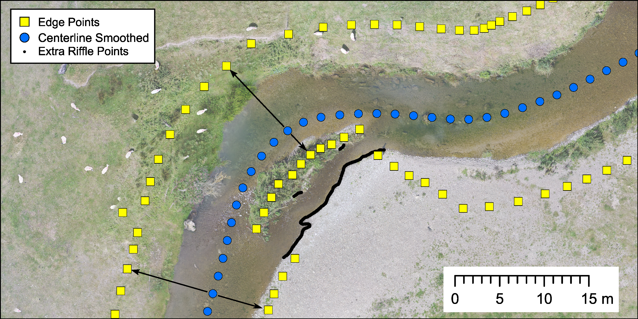
2.5. Water Surface Elevations
2.6. Refraction Correction
2.7. Small Angle Refraction Correction
2.8. Multi-View Refraction Correction (BathySfM)
2.9. Refraction Correction Validation
- 5.
- Exposed: Exposed areas only, where no refraction correction was necessary.
- 6.
- SmallAngle–Manual: Submerged areas only, using the small angle refraction correction (Equation (1)) and the manually digitised water surface elevations.
- 7.
- SmallAngle–Smooth: Submerged areas only, using the small angle refraction correction (Equation (1)) and the smoothed water surface elevations.
- 8.
- BathySfM–All: Submerged areas only, using the multi-view refraction correction and the smoothed water surface elevations.
- 9.
- BathySfM–Filtered: Submerged areas only, using the angle and distance filtered multi-view angle refraction correction and the smoothed water surface elevations.
2.10. Spatially Variable Errors
2.11. Multiple Regression
2.12. Machine Learning Classification
2.13. Error Propagation and Change Detection
3. Results
3.1. SfM Modelling
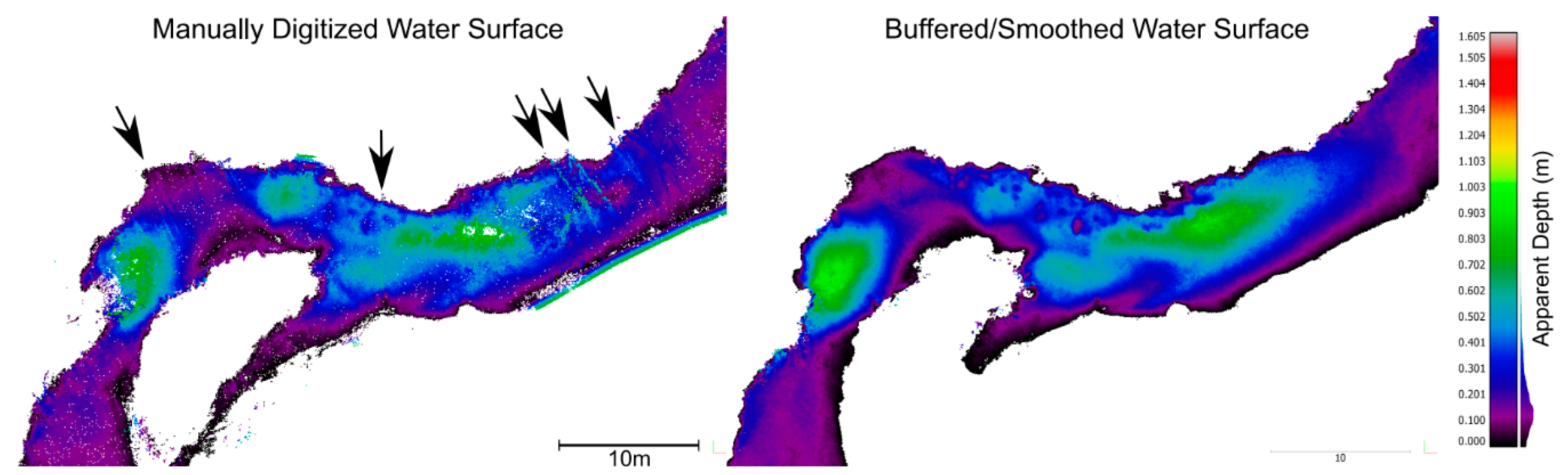
3.2. Water Surfaces
3.3. Refraction Corrections
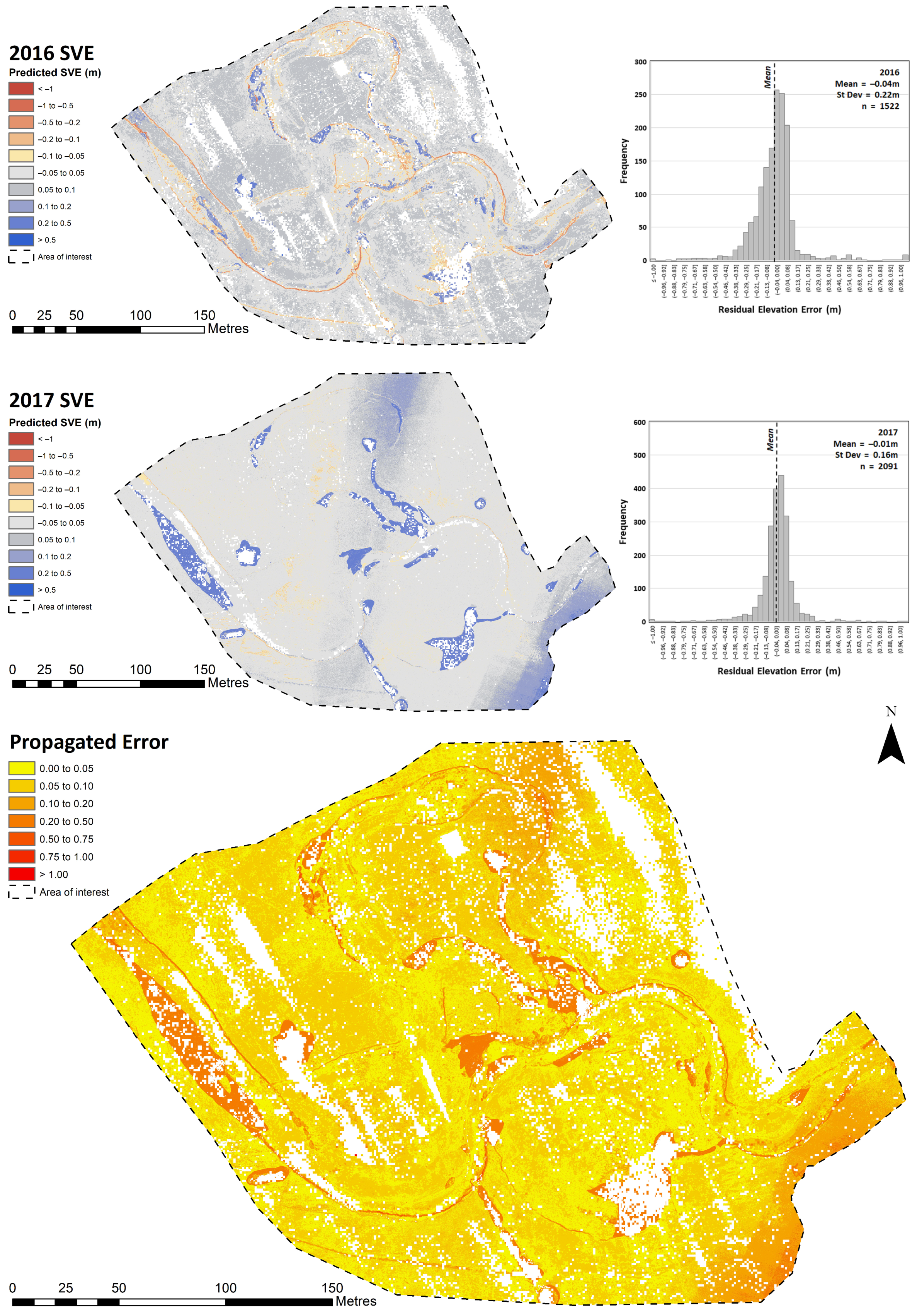
3.4. Spatially Variable Error
3.4.1. Linear Regressions
3.4.2. Multiple Regression
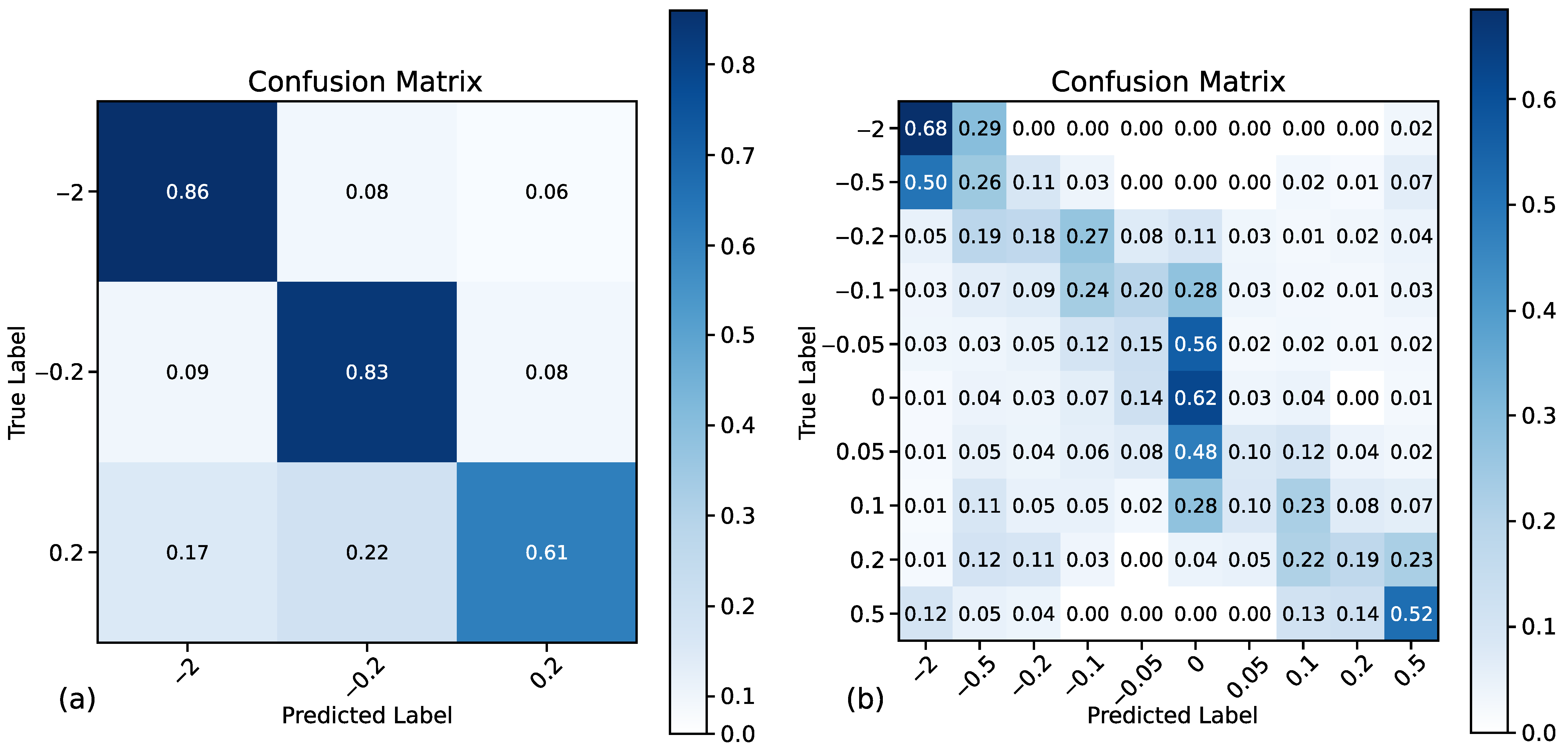
3.5. Machine Learning Classification
3.6. Geomorphic Change
4. Discussion
4.1. Refraction Correction
4.2. Water Surface Elevations
4.3. Spatially Variable Error for Geomorphic Change Detection
5. Conclusions
Author Contributions
Funding
Acknowledgments
Conflicts of Interest
References
- Wheaton, J.M.; Brasington, J.; Darby, S.E.; Sear, D.A. Accounting for uncertainty in DEMs from repeat topographic surveys: Improved sediment budgets. Earth Surf. Process. Landf. 2010, 35, 136–156. [Google Scholar] [CrossRef]
- Kociuba, W. Analysis of geomorphic changes and quantification of sediment budgets of a small Arctic valley with the application of repeat TLS surveys. Z. Fur Geomorphol. Suppl. Issues 2017, 61, 105–120. [Google Scholar] [CrossRef]
- Rice, S.; Church, M. Grain size along two gravel-bed rivers: Statistical variation, spatial pattern and sedimentary links. Earth Surf. Process. Landf. 1998, 23, 345–363. [Google Scholar] [CrossRef]
- Hodge, R.; Brasington, J.; Richards, K. In situ characterization of grain-scale fluvial morphology using Terrestrial Laser Scanning. Earth Surf. Process. Landf. 2009, 34, 954–968. [Google Scholar] [CrossRef]
- Langhammer, J.; Lendzioch, T.; Miřijovský, J.; Hartvich, F. UAV-Based Optical Granulometry as Tool for Detecting Changes in Structure of Flood Depositions. Remote Sens. 2017, 9, 240. [Google Scholar] [CrossRef]
- Woodget, A.S.; Austrums, R. Subaerial gravel size measurement using topographic data derived from a UAV-SfM approach. Earth Surf. Process. Landf. 2017, 42, 1434–1443. [Google Scholar] [CrossRef]
- Fuller, I.C.; Large, A.R.G.; Milan, D.J. Quantifying channel development and sediment transfer following chute cutoff in a wandering gravel-bed river. Geomorphology 2003, 54, 307–323. [Google Scholar] [CrossRef]
- Milan, D.J.; Heritage, G.L.; Hetherington, D. Application of a 3D laser scanner in the assessment of erosion and deposition volumes and channel change in a proglacial river. Earth Surf. Process. Landf. 2007, 32, 1657–1674. [Google Scholar] [CrossRef]
- Verhaar, P.M.; Biron, P.M.; Ferguson, R.I.; Hoey, T.B. A modified morphodynamic model for investigating the response of rivers to short-term climate change. Geomorphology 2008, 101, 674–682. [Google Scholar] [CrossRef]
- Slater, L.J.; Singer, M.B.; Kirchner, J.W. Hydrologic versus geomorphic drivers of trends in flood hazard. Geophys. Res. Lett. 2015, 42, 370–376. [Google Scholar] [CrossRef]
- Coveney, S.; Roberts, K. Lightweight UAV digital elevation models and orthoimagery for environmental applications: Data accuracy evaluation and potential for river flood risk modelling. Int. J. Remote Sens. 2017, 38, 3159–3180. [Google Scholar] [CrossRef]
- Newson, M.D.; Newson, C.L. Geomorphology, ecology and river channel habitat: mesoscale approaches to basin-scale challenges. Prog. Phys. Geogr. 2000, 24, 195–217. [Google Scholar] [CrossRef]
- Woodget, A.S.; Austrums, R.; Maddock, I.P.; Habit, E. Drones and digital photogrammetry: From classifications to continuums for monitoring river habitat and hydromorphology. Wiley Interdiscip. Rev. Water 2017, 4, e1222. [Google Scholar] [CrossRef]
- Lane, S.N.; Richards, K.S.; Chandler, J.H. Developments in monitoring and modelling small-scale river bed topography. Earth Surf. Process. Landf. 1994, 19, 349–368. [Google Scholar] [CrossRef]
- Chandler, J. Effective application of automated digital photogrammetry for geomorphological research. Earth Surf. Process. Landf. 1999, 24, 51–63. [Google Scholar] [CrossRef]
- Lane, S.N.; Westaway, R.M.; Hicks, D.M. Estimation of erosion and deposition volumes in a large, gravel-bed, braided river using synoptic remote sensing. Earth Surf. Process. Landf. 2003, 28, 249–271. [Google Scholar] [CrossRef]
- Charlton, M.E.; Large, A.R.G.; Fuller, I.C. Application of airborne LiDAR in river environments: the River Coquet, Northumberland, UK. Earth Surf. Process. Landf. 2003, 28, 299–306. [Google Scholar] [CrossRef]
- Brasington, J.; Langham, J.; Rumsby, B. Methodological sensitivity of morphometric estimates of coarse fluvial sediment transport. Geomorphology 2003, 53, 299–316. [Google Scholar] [CrossRef]
- Fausch, K.D.; Torgersen, C.E.; Baxter, C.V.; Li, H.W. Landscapes to Riverscapes: Bridging the Gap between Research and Conservation of Stream Fishes. BioScience 2002, 52, 483–498. [Google Scholar] [CrossRef]
- Harwin, S.; Lucieer, A. Assessing the Accuracy of Georeferenced Point Clouds Produced via Multi-View Stereopsis from Unmanned Aerial Vehicle (UAV) Imagery. Remote Sens. 2012, 4, 1573–1599. [Google Scholar] [CrossRef]
- Lague, D.; Brodu, N.; Leroux, J. Accurate 3D comparison of complex topography with terrestrial laser scanner: Application to the Rangitikei canyon (N-Z). ISPRS J. Photogramm. Remote Sens. 2013, 82, 10–26. [Google Scholar] [CrossRef]
- Lucieer, A.; Jong, S.M.d.; Turner, D. Mapping landslide displacements using Structure from Motion (SfM) and image correlation of multi-temporal UAV photography. Prog. Phys. Geogr. 2014, 38, 97–116. [Google Scholar] [CrossRef]
- Clapuyt, F.; Vanacker, V.; Van Oost, K. Reproducibility of UAV-based earth topography reconstructions based on Structure-from-Motion algorithms. Geomorphology 2016, 260, 4–15. [Google Scholar] [CrossRef]
- Cucchiaro, S.; Cavalli, M.; Vericat, D.; Crema, S.; Llena, M.; Beinat, A.; Marchi, L.; Cazorzi, F. Monitoring topographic changes through 4D-structure-from-motion photogrammetry: application to a debris-flow channel. Environ. Earth Sci. 2018, 77, 632. [Google Scholar] [CrossRef]
- Micheletti, N.; Chandler, J.H.; Lane, S.N. Investigating the geomorphological potential of freely available and accessible structure-from-motion photogrammetry using a smartphone. Earth Surf. Process. Landf. 2015, 40, 473–486. [Google Scholar] [CrossRef]
- Brasington, J.; Vericat, D.; Rychkov, I. Modeling river bed morphology, roughness, and surface sedimentology using high resolution terrestrial laser scanning. Water Resour. Res. 2012, 48, W11519. [Google Scholar] [CrossRef]
- Woodget, A.S.; Carbonneau, P.E.; Visser, F.; Maddock, I.P. Quantifying submerged fluvial topography using hyperspatial resolution UAS imagery and structure from motion photogrammetry. Earth Surf. Process. Landf. 2015, 40, 47–64. [Google Scholar] [CrossRef]
- Dietrich, J.T. Bathymetric Structure-from-Motion: extracting shallow stream bathymetry from multi-view stereo photogrammetry. Earth Surf. Process. Landf. 2017, 42, 355–364. [Google Scholar] [CrossRef]
- Legleiter, C.J.; Harrison, L.R. Remote Sensing of River Bathymetry: Evaluating a Range of Sensors, Platforms, and Algorithms on the Upper Sacramento River, California, USA. Water Resour. Res. 2019, 55, 2142–2169. [Google Scholar] [CrossRef]
- Vaaja, M.; Hyyppä, J.; Kukko, A.; Kaartinen, H.; Hyyppä, H.; Alho, P. Mapping Topography Changes and Elevation Accuracies Using a Mobile Laser Scanner. Remote Sens. 2011, 3, 587–600. [Google Scholar] [CrossRef]
- Schaffrath, K.R.; Belmont, P.; Wheaton, J.M. Landscape-scale geomorphic change detection: Quantifying spatially variable uncertainty and circumventing legacy data issues. Geomorphology 2015, 250, 334–348. [Google Scholar] [CrossRef]
- Miřijovský, J.; Langhammer, J. Multitemporal Monitoring of the Morphodynamics of a Mid-Mountain Stream Using UAS Photogrammetry. Remote Sens. 2015, 7, 8586–8609. [Google Scholar] [CrossRef]
- Cook, K.L. An evaluation of the effectiveness of low-cost UAVs and structure from motion for geomorphic change detection. Geomorphology 2017, 278, 195–208. [Google Scholar] [CrossRef]
- Hamshaw, S.D.; Bryce, T.; Rizzo, D.M.; O’Neil-Dunne, J.; Frolik, J.; Dewoolkar, M.M. Quantifying streambank movement and topography using unmanned aircraft system photogrammetry with comparison to terrestrial laser scanning. River Res. Appl. 2017, 33, 1354–1367. [Google Scholar] [CrossRef]
- Javemick, L.; Brasington, J.; Caruso, B. Modeling the topography of shallow braided rivers using Structure-from-Motion photogrammetry. Geomorphology 2014, 213, 166–182. [Google Scholar] [CrossRef]
- Starek, M.J.; Giessel, J. Fusion of uas-based structure-from-motion and optical inversion for seamless topo-bathymetric mapping. In Proceedings of the 2017 IEEE International Geoscience and Remote Sensing Symposium (IGARSS), Fort Worth, TX, USA, 23–28 July 2017; pp. 2999–3002. [Google Scholar]
- Flener, C.; Vaaja, M.; Jaakkola, A.; Krooks, A.; Kaartinen, H.; Kukko, A.; Kasvi, E.; Hyyppä, H.; Hyyppä, J.; Alho, P. Seamless Mapping of River Channels at High Resolution Using Mobile LiDAR and UAV-Photography. Remote Sens. 2013, 5, 6382–6407. [Google Scholar] [CrossRef]
- Tamminga, A.D.; Eaton, B.C.; Hugenholtz, C.H. UAS-based remote sensing of fluvial change following an extreme flood event. Earth Surf. Process. Landf. 2015, 40, 1464–1476. [Google Scholar] [CrossRef]
- Fonstad, M.A.; Dietrich, J.T.; Courville, B.C.; Jensen, J.L.; Carbonneau, P.E. Topographic structure from motion: a new development in photogrammetric measurement. Earth Surf. Process. Landf. 2013, 38, 421–430. [Google Scholar] [CrossRef]
- Carrivick, J.L.; Smith, M.W. Fluvial and aquatic applications of Structure from Motion photogrammetry and unmanned aerial vehicle/drone technology. Wiley Interdiscip. Rev. Water 2019, 6, e1328. [Google Scholar] [CrossRef]
- Bagheri, O.; Ghodsian, M.; Saadatseresht, M. Reach scale application of UAV+SfM methods in shallow rivers hyperspatial bathymetry. In Proceedings of the ISPRS—International Archives of the Photogrammetry, Remote Sensing and Spatial Information Sciences, Kish Island, Iran, 23–25 November 2015; Copernicus GmbH: Göttingen, Germany, 2015; Volume XL-1-W5, pp. 77–81. [Google Scholar]
- Shintani, C.; Fonstad, M.A. Comparing remote-sensing techniques collecting bathymetric data from a gravel-bed river. Int. J. Remote Sens. 2017, 38, 2883–2902. [Google Scholar] [CrossRef]
- Dietrich, J.T. pyBathySfM v4.0; GitHub: San Francisco, CA, USA, 2019. [Google Scholar] [CrossRef]
- Fisher, P.F.; Tate, N.J. Causes and consequences of error in digital elevation models. Prog. Phys. Geogr. 2006, 30, 467–489. [Google Scholar] [CrossRef]
- Sear, D.A.; Milne, J.A. Surface modelling of upland river channel topography and sedimentology using GIS. Phys. Chem. Earthpart B Hydrol. Ocean. Atmos. 2000, 25, 399–406. [Google Scholar] [CrossRef]
- Brasington, J.; Rumsby, B.T.; McVey, R.A. Monitoring and modelling morphological change in a braided gravel-bed river using high resolution GPS-based survey. Earth Surf. Process. Landf. 2000, 25, 973–990. [Google Scholar] [CrossRef]
- Jaud, M.; Grasso, F.; Le Dantec, N.; Verney, R.; Delacourt, C.; Ammann, J.; Deloffre, J.; Grandjean, P. Potential of UAVs for Monitoring Mudflat Morphodynamics (Application to the Seine Estuary, France). ISPRS Int. J. Geo-Inf. 2016, 5. [Google Scholar] [CrossRef]
- Milan, D.J.; Heritage, G.L.; Large, A.R.G.; Fuller, I.C. Filtering spatial error from DEMs: Implications for morphological change estimation. Geomorphology 2011, 125, 160–171. [Google Scholar] [CrossRef]
- James, M.R.; Robson, S.; Smith, M.W. 3-D uncertainty-based topographic change detection with structure-from-motion photogrammetry: precision maps for ground control and directly georeferenced surveys. Earth Surf. Process. Landf. 2017, 42, 1769–1788. [Google Scholar] [CrossRef]
- Seier, G.; Stangl, J.; Schöttl, S.; Sulzer, W.; Sass, O. UAV and TLS for monitoring a creek in an alpine environment, Styria, Austria. Int. J. Remote Sens. 2017, 38, 2903–2920. [Google Scholar] [CrossRef]
- Heritage, G.L.; Milan, D.J.; Large, A.R.G.; Fuller, I.C. Influence of survey strategy and interpolation model on DEM quality. Geomorphology 2009, 112, 334–344. [Google Scholar] [CrossRef]
- Chollet, F. Deep Learning with Python, 1st ed.; Manning Publications: Shelter Island, NY, USA, 2017; ISBN 978-1-61729-443-3. [Google Scholar]
- Rivas-Casado, M.; González, R.B.; Ortega, J.F.; Leinster, P.; Wright, R. Towards a Transferable UAV-Based Framework for River Hydromorphological Characterization. Sensors 2017, 17. [Google Scholar] [CrossRef]
- Buscombe, D.; Ritchie, A.C. Landscape Classification with Deep Neural Networks. Geosciences 2018, 8, 244. [Google Scholar] [CrossRef]
- Liu, T.; Abd-Elrahman, A.; Morton, J.; Wilhelm, V.L. Comparing fully convolutional networks, random forest, support vector machine, and patch-based deep convolutional neural networks for object-based wetland mapping using images from small unmanned aircraft system. GIScience Remote Sens. 2018, 55, 243–264. [Google Scholar] [CrossRef]
- Milani, G.; Volpi, M.; Tonolla, D.; Doering, M.; Robinson, C.; Kneubühler, M.; Schaepman, M. Robust quantification of riverine land cover dynamics by high-resolution remote sensing. Remote Sens. Environ. 2018, 217, 491–505. [Google Scholar] [CrossRef]
- Boonpook, W.; Tan, Y.; Ye, Y.; Torteeka, P.; Torsri, K.; Dong, S. A Deep Learning Approach on Building Detection from Unmanned Aerial Vehicle-Based Images in Riverbank Monitoring. Sensors 2018, 18. [Google Scholar] [CrossRef] [PubMed]
- Baron, J.; Hill, D.J.; Elmiligi, H. Combining image processing and machine learning to identify invasive plants in high-resolution images. Int. J. Remote Sens. 2018, 39, 5099–5118. [Google Scholar] [CrossRef]
- Heritage, G.L.; Hemsworth, M.; Hicks, L. Restoring the River Teme SSSI: A River Restoration Plan—Technical Report Draft (v4.2); JBA for Natural England: Skipton, UK, 2013. [Google Scholar]
- James, M.R.; Robson, S. Mitigating systematic error in topographic models derived from UAV and ground-based image networks. Earth Surf. Process. Landf. 2014, 39, 1413–1420. [Google Scholar] [CrossRef]
- Wackrow, R.; Chandler, J.H. Minimising systematic error surfaces in digital elevation models using oblique convergent imagery. Photogramm. Rec. 2011, 26, 16–31. [Google Scholar] [CrossRef]
- Chandler, J.H.; Fryer, J.G.; Jack, A. Metric capabilities of low-cost digital cameras for close range surface measurement. Photogramm. Rec. 2005, 20, 12–26. [Google Scholar] [CrossRef]
- Legleiter, C.J.; Kyriakidis, P.C. Forward and Inverse Transformations between Cartesian and Channel-fitted Coordinate Systems for Meandering Rivers. Math. Geol. 2006, 38, 927–958. [Google Scholar] [CrossRef]
- Olson, R.S.; Urbanowicz, R.J.; Andrews, P.C.; Lavender, N.A.; Kidd, L.C.; Moore, J.H. Automating Biomedical Data Science through Tree-Based Pipeline Optimization. In Applications of Evolutionary Computation, Proceedings of EvoApplications 2016; Springer: Berlin, Germany, 2016. [Google Scholar]
- Pedregosa, F.; Varoquaux, G.; Gramfort, A.; Michel, V.; Thirion, B.; Grisel, O.; Blondel, M.; Prettenhofer, P.; Weiss, R.; Dubourg, V.; et al. Scikit-learn: Machine Learning in Python. J. Mach. Learn. Res. 2011, 12, 2825–2830. [Google Scholar]
- Chawla, N.V.; Bowyer, K.W.; Hall, L.O.; Kegelmeyer, W.P. SMOTE: Synthetic Minority Over-sampling Technique. J. Artif. Intell. Res. 2002, 16, 321–357. [Google Scholar] [CrossRef]
- Lemaître, G.; Nogueira, F.; Aridas, C.K. Imbalanced-learn: A Python Toolbox to Tackle the Curse of Imbalanced Datasets in Machine Learning. J. Mach. Learn. Res. 2017, 18, 559–563. [Google Scholar]
- Mapbox. Rasterio v1.0. 2018. Available online: https://github.com/mapbox/rasterio (accessed on 12 December 2018).
- van der Walt, S.; Colbert, S.C.; Varoquaux, G. The NumPy Array: A Structure for Efficient Numerical Computation. Comput. Sci. Eng. 2011, 13, 22–30. [Google Scholar] [CrossRef]
- McKinney, W. Data Structures for Statistical Computing in Python. In Proceedings of the 9th Python in Science Conference, Austin, TX, USA, 28 June–3 July 2010; pp. 51–56. [Google Scholar] [CrossRef]
- Hunter, J.D. Matplotlib: A 2D Graphics Environment. Comput. Sci. Eng. 2007, 9, 90–95. [Google Scholar] [CrossRef]
- Kluyver, T.; Ragan-Kelley, B.; Pérez, F.; Granger, B.E.; Bussonnier, M.; Frederic, J.; Kelley, K.; Hamrick, J.B.; Grout, J.; Corlay, S.; et al. Jupyter Notebooks-a publishing format for reproducible computational workflows. In Proceedings of the 20th International Conference on Electronic Publishing, Göttingen, Germany, 9 June 2016; pp. 87–90. [Google Scholar]
- Wilson, R.T.; Woodget, A.S. Code for Woodget, Dietrich and Wilson; GitHub: San Francisco, CA, USA, 2019. [Google Scholar] [CrossRef]
- Carbonneau, P.E.; Dietrich, J.T. Cost-effective non-metric photogrammetry from consumer-grade sUAS: Implications for direct georeferencing of structure from motion photogrammetry. Earth Surf. Process. Landf. 2017, 42, 473–486. [Google Scholar] [CrossRef]
- Buscombe, D. SediNet: A configurable deep learning model for mixed qualitative and quantitative optical granulometry. EarthArXiv 2019. [Google Scholar] [CrossRef]


| Parameter (Type) | Symbol | Method of Extraction | Type: Range/Units | Sample Size: Count (%) | |
|---|---|---|---|---|---|
| 2016 | 2017 | ||||
| Slope angle (topographic complexity) | S | RPAS–SfM DEMs imported to ArcGIS. 3D Analyst extension was used to compute slope angles. Focal (f) statistics for slope within a 0.2 m circular window of each validation point also computed. | Continuous: 0–90° | 1522 (100%) | 2091 (100%) |
| Point cloud roughness (topographic complexity) | R | RPAS–SfM point clouds imported to CloudCompare. ‘Compute geometric features’ tool used to compute roughness for each point in the cloud within spherical kernels with a 0.4 m radius. Roughness is defined as the distance between the point and the best fitting plane computing from all the surrounding points which fall within the kernel. Rasterised at 0.1 m pixel size and exported to ArcGIS. Smaller pixel sizes were found to produce too many holes in the resulting raster. Focal statistics for roughness within a 0.2 m circular window of each validation point also computed. | Continuous: 0–0.34 m | 1515 (99.5%) | 2090 (99.9%) |
| Point cloud density (survey quality/ landscape composition) | D | RPAS–SfM point clouds imported to CloudCompare and rasterised according to the number of points falling within each 0.05 m grid cell. Raster exported to ArcGIS. | Continuous: 0–64 count | 1522 (100%) | 2091 (100%) |
| Water depth (landscape composition) | h | Computed using the multi-view refraction correction process and smoothed water surface, as detailed within this paper (BathySfM–All). | Continuous: 0–1.97 m | 355 (23.3%) | 1170 (56%) |
| Image quality (survey quality) | CQ | Image quality estimates are provided by PhotoScan Pro on a scale of 0 to 1 and based on the level of image sharpness in the best focused area of the image. Images with quality values of less than 0.5 are generally not recommended for use in subsequent processing. Image quality data were exported from PhotoScan Pro and the average quality of cameras that ‘see’ each point was appended to that point. Point–camera connections were calculated in the same way as the BathySfM correction. | Continuous: 0–1 | 1522 (100%) | 2086 (99.8%) |
| Tie point precision (survey quality/ landscape composition) | P | Computed using the tie point precision method presented by [49]. Tie points are rasterised at 1 m pixel size and exported from CloudCompare to ArcGIS. The tie points form the sparse point cloud from the PhotoScan Pro software, therefore exporting at a finer resolution would lead to large holes in the resulting raster. | Continuous: 0–4.8 m | 1342 (88.2%) | 1884 (90.1%) |
| Vegetation presence (landscape composition) | V | RPAS–SfM orthophotos imported to ArcGIS. Editor toolbar used to visually identify and map areas of particularly dense vegetation or tree coverage. | Binary: [0] = Not present [1] = Present | 1522 (100%) [0] = 89.5% [1] = 10.5% | 2091 (100%) [0] = 90.5% [1] = 9.5% |
| Presence of water surface reflection (survey conditions) | Rc | RPAS–SfM orthophotos imported to ArcGIS. Editor toolbar used to visually identify and map areas of notable water surface reflections. | Binary: [0] = Not present [1] = Present | 1522 (100%) [0] = 98% [1] = 2% | 2091 (100%) [0] = 94.3% [1] = 5.7% |
| Presence of shadows (survey conditions) | Sh | RPAS–SfM orthophotos imported to ArcGIS. Editor toolbar used to visually identify and map areas of dark shadowing. | Binary: [0] = Not present [1] = Present | 1522 (100%) [0] = 99.5% [1] = 0.5% | 2091 (100%) [0] = 98.3% [1] = 1.7% |
| Mean | St Dev | 95% Conf. | RMSE | MIN | MAX | ||
|---|---|---|---|---|---|---|---|
| 2016 | X | 0.000 | 0.021 | 0.041 | 0.020 | –0.047 | 0.030 |
| Y | 0.000 | 0.027 | 0.052 | 0.026 | –0.046 | 0.047 | |
| Z | –0.001 | 0.017 | 0.034 | 0.017 | –0.029 | 0.035 | |
| 2017 | X | 0.000 | 0.035 | 0.068 | 0.034 | –0.054 | 0.056 |
| Y | 0.000 | 0.059 | 0.116 | 0.057 | –0.096 | 0.076 | |
| Z | 0.000 | 0.006 | 0.013 | 0.006 | –0.018 | 0.006 |
| 2016 | 2017 | |||||||||
|---|---|---|---|---|---|---|---|---|---|---|
| Correction Method | (1) Exposed Only | (2) Small Angle– Manual | (3) Small Angle– Smooth | (4) Bathy SfM–All | (5) Bathy SfM–Filtered | (1) Exposed Only | (2) Small Angle– Manual | (3) Small Angle– Smooth | (4) Bathy SfM–All | (5) Bathy SfM–Filtered |
| Mean Error | 0.024 | 0.150 | 0.041 | 0.016 | 0.027 | 0.065 | 0.034 | 0.017 | –0.055 | 0.006 |
| St Dev of Error | 0.235 | 0.205 | 0.065 | 0.061 | 0.062 | 0.226 | 0.105 | 0.079 | 0.101 | 0.079 |
| Regression Slope | 0.942 | 0.915 | 0.997 | 0.989 | 0.992 | 0.940 | 0.903 | 1.068 | 1.057 | 1.060 |
| Min Error | –1.710 | -0.645 | –0.130 | –0.156 | –0.152 | –1.235 | –0.293 | –0.269 | –0.439 | –0.282 |
| Max Error | 1.097 | 1.403 | 0.501 | 0.445 | 0.482 | 1.566 | 2.261 | 0.520 | 0.485 | 0.513 |
| (a) Elevation Error—Magnitude and Direction | (b) Elevation Error—Magnitude Only | |||||
|---|---|---|---|---|---|---|
| Variable | Combined | 2016 | 2017 | Combined | 2016 | 2017 |
| Slope | –0.10 | –0.20 | 0.00 | 0.50 | 0.47 | 0.56 |
| Max. Slope Focal | –0.12 | –0.24 | 0.00 | 0.52 | 0.53 | 0.53 |
| Min. Slope Focal | –0.06 | –0.09 | –0.03 | 0.37 | 0.39 | 0.39 |
| St. Dev. Slope Focal | –0.12 | –0.25 | 0.04 | 0.44 | 0.44 | 0.45 |
| Water Depth (BathySfM–All) | –0.05 | 0.01 | –0.11 | –0.15 | –0.10 | –0.19 |
| Point Density | –0.12 | –0.14 | –0.10 | 0.28 | 0.23 | 0.43 |
| Image Quality Mean | –0.04 | –0.01 | –0.07 | 0.05 | 0.07 | 0.02 |
| Image Quality Mean Focal | –0.04 | –0.01 | –0.07 | 0.06 | 0.07 | 0.02 |
| Roughness 40 cm | –0.04 | –0.17 | 0.12 | 0.31 | 0.22 | 0.41 |
| Roughness 40 cm Focal | –0.05 | –0.19 | 0.14 | 0.38 | 0.30 | 0.49 |
| Tie Point Precision | 0.05 | 0.02 | 0.07 | 0.06 | 0.14 | 0.06 |
| (a) Elevation Error—Magnitude and Direction | (b) Elevation Error—Magnitude Only | |||||
|---|---|---|---|---|---|---|
| Performance Variable | Combined | 2016 | 2017 | Combined | 2016 | 2017 |
| Multiple R | 0.47 | 0.54 | 0.53 | 0.61 | 0.65 | 0.63 |
| Adjusted R Square | 0.22 | 0.29 | 0.28 | 0.37 | 0.42 | 0.40 |
| Standard Error (m) | 0.17 | 0.18 | 0.14 | 0.13 | 0.14 | 0.11 |
| Significance (p-value) | <0.01 | <0.01 | <0.01 | <0.01 | <0.01 | <0.01 |
| Slope (obs vs. pred) | NC | 0.1666 | 0.1297 | NC | NC | NC |
| Mean Residual Error (m) | NC | –0.04 | –0.01 | NC | NC | NC |
| Max Residual Error (m) | NC | 1.48 | 1.09 | NC | NC | NC |
| Min Residual Error (m) | NC | –4.48 | –1.23 | NC | NC | NC |
| St Dev Residual Error (m) | NC | 0.22 | 0.16 | NC | NC | NC |
| Variable | Standard Deviation | Multiple Regression Co-Efficients/Intercept | |
|---|---|---|---|
| Epochs Combined | 2016 | 2017 | |
| Maximum Slope Focal (MaxSf) | 20.3411 | –0.0674 | –0.0281 |
| Minimum Slope Focal (MinSf) | 5.4814 | –0.0059 | –0.0034 |
| Refraction Corrected Water Depth (h) | 0.2061 | 0.0140 | –0.0228 |
| Point Cloud Density (D) | 4.1113 | –0.0071 | –0.0747 |
| Mean Image Quality Focal (MeanCQf) | 1.9848 | –0.0010 | –0.0266 |
| Mean Roughness Focal (MeanRf) | 0.0150 | –0.0212 | 0.0333 |
| Point Cloud Precision (P) | 0.3863 | 0.0437 | 0.0019 |
| Presence of Vegetation (V) | N/A | 0.2604 | 0.2354 |
| Presence of Shadows (Sh) | N/A | –0.4588 | 0.0616 |
| Presence of Reflections (Rc) | N/A | 0.0511 | 0.0084 |
| Intercept (θ) | N/A | 0.1533 | 1.1812 |
| Classes | Epoch | Accuracy | F1 Score |
|---|---|---|---|
| 3 classes | 2016 | 78% | 0.83 |
| 2017 | 76% | 0.81 | |
| Both | 74% | 0.80 | |
| 10 classes | 2016 | 26% | 0.22 |
| 2017 | 31% | 0.30 | |
| Both | 29% | 0.27 |
| This Paper | Flener et al. [37] | Tamminga et al. [38] | Shintani and Fonstad [42] | |
|---|---|---|---|---|
| Refraction correction approach | Co-efficient for clear water (1.34): Small angle & multiview | Optical calibration | Optical calibration | Site specific co-efficient |
| Calibration data needed? | No | Yes | Yes | Yes |
| Validation points | 1522–2093 | 197 GPS points + extra ADCP points (not reported) | 76–82 | 167 |
| Survey size | 600 m reach | ca. 150 m reach (20–30 m wide) | 800 m reach | 140 m reach |
| Validation survey type | Differential GNSS + total station | RTK GPS + ADCP | RTK GPS | RTK GPS |
| Validation point layout | Random distribution over a range of water depths | Zig-zag pattern along channel over range of water depths | Not reported | 12 evenly spaced channel cross sections |
| Maximum water depth (m) | 1.43 | 1.50 | Not reported | 1.25 |
| Mean error (m) | 0.006–0.041 | 0.117–0.1196 | 0.0001–0.0007 | 0.009 |
| RMSE (m) | 0.063–0.115 | 0.163–0.221 | 0.095–0.098 | Not reported |
| Standard deviation (m) | 0.061–0.101 | Not reported | 0.009–0.023 | 0.172 |
© 2019 by the authors. Licensee MDPI, Basel, Switzerland. This article is an open access article distributed under the terms and conditions of the Creative Commons Attribution (CC BY) license (http://creativecommons.org/licenses/by/4.0/).
Share and Cite
Woodget, A.S.; Dietrich, J.T.; Wilson, R.T. Quantifying Below-Water Fluvial Geomorphic Change: The Implications of Refraction Correction, Water Surface Elevations, and Spatially Variable Error. Remote Sens. 2019, 11, 2415. https://doi.org/10.3390/rs11202415
Woodget AS, Dietrich JT, Wilson RT. Quantifying Below-Water Fluvial Geomorphic Change: The Implications of Refraction Correction, Water Surface Elevations, and Spatially Variable Error. Remote Sensing. 2019; 11(20):2415. https://doi.org/10.3390/rs11202415
Chicago/Turabian StyleWoodget, Amy S., James T. Dietrich, and Robin T. Wilson. 2019. "Quantifying Below-Water Fluvial Geomorphic Change: The Implications of Refraction Correction, Water Surface Elevations, and Spatially Variable Error" Remote Sensing 11, no. 20: 2415. https://doi.org/10.3390/rs11202415
APA StyleWoodget, A. S., Dietrich, J. T., & Wilson, R. T. (2019). Quantifying Below-Water Fluvial Geomorphic Change: The Implications of Refraction Correction, Water Surface Elevations, and Spatially Variable Error. Remote Sensing, 11(20), 2415. https://doi.org/10.3390/rs11202415