A Novel Hyperspectral Image Simulation Method Based on Nonnegative Matrix Factorization

Abstract

Hyperspectral (HS) images can provide abundant and fine spectral information on land surface. However, their applications may be limited by their narrow bandwidth and small coverage area. In this paper, we propose an HS image simulation method based on nonnegative matrix factorization (NMF), which aims at generating HS images using existing multispectral (MS) data. Our main novelty is proposing a spectral transformation matrix and new simulation method. First, we develop a spectral transformation matrix that transforms HS endmembers into MS endmembers. Second, we utilize an iteration scheme to optimize the HS and MS endmembers. The test MS image is then factorized by the MS endmembers to obtain the abundance matrix. The result image is constructed by multiplying the abundance matrix by the HS endmembers. Experiments prove that our method provides high spectral quality by combining prior spectral endmembers. The iteration schemes reduce the simulation error and improve the accuracy of the results. In comparative trials, the spectral angle, RMSE, and correlation coefficient of our method are 5.986, 284.6, and 0.905, respectively. Thus, our method outperforms other simulation methods.

1. Introduction

Hyperspectral (HS) remote sensing technology can acquire a wide-wavelength-range and fine spectral information of an observation area through numerous spectral channels. The abundant spectral information enables widespread applications, such as soil contamination [1], geological mineral mapping [2], fire detection [3], and vegetation monitoring [4]. However, the coverage area and observation time restrict wider applications of HS images [5]. For example, the well-known HS sensor Hyperion has a swath width of 7.5 km, which is considerably narrower than that of other satellite images [6]. The observed objects in a scene are significantly decreased. Meanwhile, the visit cycle of Hyperion is 200 days, which limits the application of Hyperion data [7]. For cloudy areas, the data collection will be further difficult because of the long revisiting period [8,9]. Therefore, HS images are still difficult to obtain from large-area and more frequent coverages. In comparison with HS images, multispectral (MS) data have the advantages of economic accessibility, frequent observation, and global coverage [10]. Furthermore, MS images can be provided by numerous satellites, such as Sentinel-2 [11], Proba-V [12], ALOS [13], and Landsat series [14], which have accumulated massive and long-term historical record of land surface data. Hence, a simulation method must be designed to generate HS images on the basis of the existing MS data of the study area. With these simulated HS images, the application fields of the HS technology can be extended in land cover mapping [15], soil monitoring [16], and agriculture management [17].

Many HS image simulation methods have been developed in the past decades. Chen et al. first proposed such an approach using the HS libraries of Johns Hopkins University (JHU) [18]. The MS data were first classified by spectral similarity referring to the data in the JHU library. According to the classification result, the MS information of each pixel is corresponded to a detailed spectrum of the same class in the library. The simulated HS image is subsequently produced by replacing the MS information with the corresponding HS information. This method is easy to implement. However, as the HS images are built on the basis of some standard spectrums, the other types of objects are not well considered [5]. It is difficult to present the actual surface details. Meanwhile, the misclassifications of pixels may reduce the quality of the results [18].

On the basis of the linear spectrum unmixing model, Liu et al. developed a universal pattern decomposition method (UPDM) [19]. This method initially uses the unmixing model to decompose each pixel in the MS image into the standard MS spectrums of water, vegetable, soil, and a supplementary one. The standard MS spectrums are produced by downsampling the standard HS spectrums. Then, the decomposition coefficients of each class are linearly combined with the corresponding HS spectrums to reconstruct the HS information. After the HS information of all the pixels are reconstructed, the result is output as the simulated HS image. The UPDM performs efficiently in simple scenes. However, complex scenes with distribution of various materials are difficult to be produced accurately due to the small number of reference spectrums [5]. Moreover, the standard spectrums may be slightly different from the actual spectrums in the image; as such, this approach is influenced by the actual environment [19].

Winter et al. designed another framework, namely, color resolution improvement software package (CRISP) [20,21]. This approach constructs multivariate linear functions to transform MS data into HS data. The coefficients of functions are calculated using a multiple linear regression model between the MS data and each band of the training HS data. Then, each HS band is simulated using the MS image with obtained band coefficients. Following this idea, Sun et al. extracted spectrums of different classes from MS and HS images to calculate the corresponding transformation functions [10]. Subsequently, the suitable function of each pixel was found using a spectral angle weighted minimum distance matching method. The HS data were produced by utilizing the selected functions to transform the MS information of the pixels into HS information. Hoang et al. further proposed a pseudo-hyperspectral image transformation algorithm (PHITA), which considers the correlations between MS and HS bands. The PHITA selects the highly correlated MS channels through Bayesian model averaging [5]. Each HS band is constructed using a multiple linear regression model and the most suitable MS bands. The CRISP-based methods may produce large distortions in heterogeneous areas [5] because the pixels with complex and special spectral information are difficult to generate accurately by the transforming functions of global images.

Both previous studies can provide simulated HS images with large coverage on the basis of MS data. However, the abovementioned drawbacks of these studies, such as the misclassification, small number of reference spectrums and large spectral distortion in complex areas, severely reduce the accuracy of the results. Therefore, a method that can accurately estimate HS images in areas with complex and multi-class objects is still needed. The nonnegative matrix factorization (NMF) of images is a promising and effective method that has been widely used in image fusion [22,23,24], super-resolution [25,26,27], spectral estimation [28], and unmixing [29,30,31]. This method linearly combines the spectral endmembers and their corresponding coefficients to produce each pixel of the result image. In this process, the spectral endmembers are formed as an endmember matrix, and the coefficients are formed as an abundance matrix. NMF has advantages in simultaneously determining endmembers and coefficients without the need of pure pixel assumption [29].

In this paper, we propose an HS image simulation method based on NMF. Our main contribution is designing a novel spectral transformation matrix and new HS image simulation method. First, we represent the relation between each MS band and the corresponding HS bands as a multivariate linear model. The obtained coefficients compose our spectral transformation matrix, which can transform the HS endmembers into MS ones. Then, we develop the new simulation method based on the coupled NMF [32] to factorize the HS and MS images. The final simulated HS image is produced by combining the abundance matrix of the MS image and the HS endmember matrix.

This paper is organized as follows. Section 2 initially introduces the experimental datasets and then discusses the novel spectral transformation matrix and proposed HS image simulation method. Section 3 presents the experiments and results on four datasets and reports the comparisons between the proposed and other methods. Section 4 provides additional discussions about our approach and a detailed parameter analysis. Finally, Section 5 draws the conclusions.

2. Materials and Methods

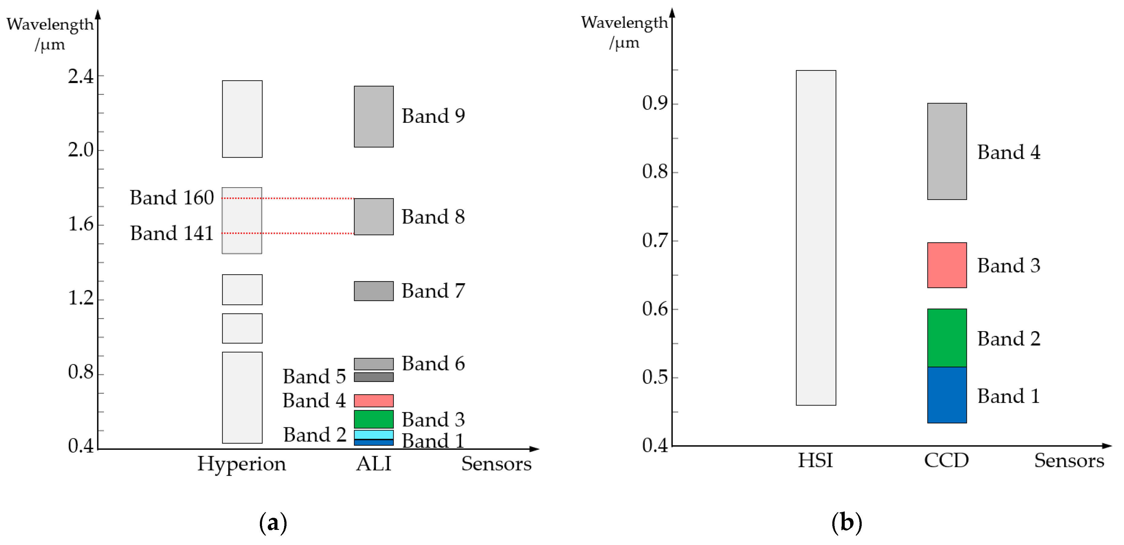
2.1. Datasets

In this paper, four datasets from Earth Observation-1 (EO-1) and Huangjing-1A (HJ-1A) satellites are selected as experimental data. Each dataset contains HS and MS images of the same area. The first dataset covers Hongkong City, with dense buildings, abundant vegetation, and sea. The second dataset covers Longyan City in Fujian Province, with urban, mining, and vegetated areas. The third dataset presents a suburban area of Wuhan in the middle of China, with agriculture regions, and a part of the Yangtze River. The fourth dataset locates near Baotou, with agriculture and mountain areas in the north of China. The training and test images of Dataset 4 are not from the same scene, which could provide cross validation of the simulation methods. Figure 1 shows the geographic locations of the images in Dataset 4.

Table 1. Detailed information of the test datasets.

Dataset	Sizes	Spatial Resolution	Training Area	Bands	Satellite & Sensors	Longitude/°E	Latitude/°N
1	MS 180 × 2000	30 m	180 × 400	9	EO-1 (ALI)	114.22–114.28	22.33–25.87
	HS 180 × 2000	30 m		154	EO-1 (Hyperion)
2	MS 318 × 480	30 m	318 × 100	4	HJ-1A (CCD)	116.25–116.57	24.89–25.32
	HS 95 × 144	100 m		92	HJ-1A (HSI)
3	MS 150 × 1850	30 m	150 × 370	9	EO-1 (ALI)	113.96–114.00	29.95–30.45
	HS 150 × 1850	30 m		154	EO-1 (Hyperion)
4	MS 180 × 600	30 m	200 × 500	9	EO-1 (ALI)	109.45–109.74	40.44–41.08
	HS 180 × 600	30 m		154	EO-1 (Hyperion)

presents further detailed information about the test datasets. The test datasets can objectively validate the performance of the proposed method in different environments.

In Datasets 1, 3 and 4, the Hyperion data provide 242 bands with the wavelength ranges from 0.356 μm to 2.577 μm [7]. However, some bands produce a considerable amount of noise because of the malfunction in the Hyperion sensor. We manually select 154 bands (10th−57th, 80th−120th, 134th−164th, 187th−220th bands) with good quality to compose the test HS image [33,34]. The ALI data covers the wavelength range from 0.433 μm to 2.35 μm by 9 bands. All the bands of ALI data are used in our experiments. In Dataset 2, the original HSI data contains 115 bands. The wavelength ranges from 0.45 μm to 0.95 μm. We also selected 92 bands (21st−112th bands) with little noise as our experiment HS data. The CCD data covers a 0.43–0.9 μm wavelength range. All the 4 bands in CCD data are contained in the test MS image. Before experiments, all the test images are preprocessed by the commercial software ENVI 5.3. The preprocessing steps include radiation calibration, atmospheric correction and image registration. More detailed information about the spectral wavelengths of the sensors are presented in Figure 2.

2.2. Methods

Figure 3 presents an overview of our proposed method. We prepare MS and overlapped HS images. A small subarea in the MS image and the corresponding area in the HS image are extracted as the training MS and HS images, respectively. The rest of the MS image is the test MS image, which is used to simulate the HS image. In our method, the simulated images are produced by combining an HS endmember matrix and an abundance matrix. First, we extract HS endmembers from the training HS image and obtain corresponding MS endmembers through spectral transformation matrix. The spectral transformation matrix is estimated using the proposed method in Section 2.2.2. Second, we use the iteration computations of coupled NMF to update the MS and HS endmembers alternately. The iteration scheme improves the accuracy of the HS and MS endmembers in the factorization of the HS and MS images. Afterward, we utilize the updated MS endmembers to factorize the test MS image through a new round of iterations based on multiplicative update rules. The abundance matrix of the test MS image is then achieved. The simulated HS image is produced by multiplying the achieved abundance matrix by the updated HS endmember matrix.

In this part, Section 2.2.1 reviews the nonnegative matrix factorization of images. The estimation of the spectral transformation matrix is presented in Section 2.2.2. The iteration schemes of image simulation are introduced in detail in Section 2.2.3.

2.2.1. Nonnegative Matrix Factorization of Images

Each pixel in the remote sensing image covers an area on the ground. The covered area often contains multiple classes of materials due to the complex distribution of ground objects. Each material has a typical spectrum. Therefore, the spectral information in a pixel can be divided into several types of basic pure spectrums. The linear spectral unmixing model has been widely used to represent the relationship between pixel and basic spectrums [35]. This model assumes that each pixel can be approximated to a weighted sum of several pure spectrums of different materials. In many previous studies, the pure spectrums and their corresponding weight coefficients are known as spectral endmembers and abundance [35,36]. The mathematical expression of the linear spectral unmixing model is as follows:

$$p=c_1{e}_1+c_2{e}_2+\cdots +c_n{e}_n+r$$

(1)

where $p$ is the pixel in the remote sensing image, $e_i$ is the spectral endmembers, $n$ is the number of endmembers, $c_i$ represents the weight coefficient of each endmember, and $r$ is the residual. The linear spectral unmixing model has advantages of intuitive interpretation, sufficient accuracy, and simplicity [37].

By using the linear spectral unmixing model, each pixel in images can be decomposed into a group of endmembers and their abundance. Equation (1) is rewritten in matrix form as

$$\mathit{P}=\mathit{E}\mathit{C}+\mathit{N},$$

(2)

where $\mathit{P}={\left(p_1,\dots ,p_{\lambda }\right)}^T\in {ℝ}^{\lambda \times 1}$ is a pixel with $\lambda$ bands. $\mathit{E}\in {ℝ}^{\lambda \times n}$ is the endmember matrix with $n$ endmembers, in which each column is an endmember spectrum. $\mathit{C}={\left(c_1,\dots ,c_n\right)}^T\in {ℝ}^{n\times 1}$ is the abundance matrix, where $c_i$ denotes the abundance value of the ith endmember. $\mathit{N}={\left(r_1,\dots ,r_{\lambda }\right)}^T\in {ℝ}^{\lambda \times 1}$ is the residual matrix. Generally, the abundance is interpreted as the area proportions of materials in a pixel.

The physical meaning indicates that the abundance matrix should be constrained by two conditions: (1) all elements in matrix $\mathit{C}$ are nonnegative and (2) the sum of any row in $\mathit{C}$ is one.

Remote sensing image is composed of numerous pixels. To factorize an image, we initially arrange the image in a new matrix with the size of $\mathsf{\lambda }\times L$. $L$ denotes the number of pixels in the image. Subsequently, the image is transformed from a 3D matrix to a 2D one. Each column represents a pixel with $\mathsf{\lambda }$ channels. The abundance of the pixel is a column vector. To represent the abundance of all pixels, we increase the number of columns in the abundance matrix. Then, the image matrix can be reconstructed by multiplying an endmember matrix with a 2D abundance matrix

$$u\approx \mathit{E}\mathit{C},$$

(3)

where $u\in {ℝ}^{\mathsf{\lambda }\times L}$ denotes the rearranged image, $\mathit{E}\in {ℝ}^{\lambda \times n}$ is the endmember matrix, and $\mathit{C}\in {ℝ}^{n\times L}$ represents the abundance matrix of the image. The residual $\mathit{N}\in {ℝ}^{\mathsf{\lambda }\times L}$ is ignored.

2.2.2. Estimation of Spectral Transformation Matrix

In the HS image simulation problem, the simulated HS image is constructed on the basis of a test MS image of the same area. The distributions of ground objects are the same in the HS and MS images. Therefore, each pixel in HS image should contain similar materials and proportions to the corresponding pixel in the MS image. If endmembers of the same group of materials are used to unmix the HS and MS images, then the abundance matrix of the HS image should be equal to that of the MS image. We assume that the simulated HS image can be obtained by multiplying the HS endmember matrix by the MS abundance matrix. On the basis of this hypothesis, we must build the transformation relation between the endmember matrixes of the HS and MS images.

HS images can provide wide and continuous ranges of spectral information. As one of the well-known HS sensors, Hyperion covers a 356–2577 nm wavelength range [38]. Meanwhile, the high spectral resolution (10 nm) makes Hyperion image contain 242 bands [38]. The wavelength ranges of MS images are more discrete and considerably narrower than those of HS images. For example, the MS sensor Advanced Land Imagery (ALI) provides discrete wavelength coverage in nine bands. Figure 2a presents an intuitive comparison between wavelength ranges of Hyperion and ALI data.

As presented in Figure 2, the wavelength range of the bands in MS image is divided into many small spectral ranges in HS image. The HS bands can be seen as fine divisions of the MS channels. We assume that an MS band can be obtained by linearly combining the HS bands in the same wavelength range with the target MS band. For example, the 8th band of the ALI image can be reconstructed using the 141th–160th bands of the Hyperion image (Figure 2a). We do not utilize the other bands in HS image, outside the range of 141th–160th, in this reconstruction. The reason is that the wavelength range of the other bands is excluded in the range of the target MS band. The spectral features acquired by the other HS bands may not be contained in this target MS band. Therefore, only HS bands in the same wavelength range are selected to produce the corresponding MS channel. The assumption is formulized as

$$M_i=w_{i1}{H}_j+\cdots +w_{it}{H}_{j+t}+r_i,$$

(4)

where $M_i$ is the produced MS band, $H_j\dots H_{j+t}$ are the HS channels in the given wavelength ranges, $w_{i1}\dots w_{it}$ denote the weights of each channel, and $r_i$ is the residual. Then, we need to estimate the weights of the HS channels. The multiple linear regression model is selected in our approach.

We initially use the training HS and MS images to develop the multiple linear regression model. The relation function is constructed as

$$u_{mi}=W_i{u}_{hj}+N_i,$$

(5)

where $u_{mi}\in {ℝ}^{1\times L}$ is the training MS channel rearranged in a $1\times L$ matrix, $u_{hj}\in {ℝ}^{t\times L}$ is the training HS bands rearranged in a $t\times L$ matrix, $W_i\in {ℝ}^{1\times t}$ is the weight matrix that need to be estimated, and $N_i$ is the residual. The weight matrix can be estimated using the linear regression model:

$$W_i={\left[{\left(u_{hj}{u}_{hj}^T\right)}^{-1}{u}_{hj}{u}_{mi}^T\right]}^T.$$

(6)

Following this strategy, the weight matrix of each MS band can be obtained. We integrate the weight matrixes of all MS channels as an overall matrix.

$$\mathit{W}=\left[\begin{array}{cccc}{W}_1& 0& \cdots & 0\\ 0& W_2& & \\ ⋮& & \ddots & 0\\ 0& \cdots & 0& W_m\end{array}\right],$$

(7)

where $\mathit{W}\in {ℝ}^{m\times h}$ and $m$ is the number of bands in the MS image. In our method, $\mathit{W}$ is the spectral transformation matrix, which can realize the spectral degradation of the global HS image. Finally, we can use the spectral transformation matrix to build the image relation function:

$$u_m\approx \mathit{W}{u}_h,$$

(8)

where $u_m\in {ℝ}^{m\times L}$ and $u_h\in {ℝ}^{h\times L}$ are the rearranged training MS and HS images, respectively. $h$ denotes the number of channels in the HS image, and the residual is ignored.

In addition, it is worth noting that not all the MS channels are included in the wavelength range of the simulated HS image. For instance, the HS data acquired by Huanjing-1A satellite (HJ-1A) covers the wavelength from 450 nm to 950 nm [39]. When we use Landsat MS images to simulate the HJ-1A HS data, the shortwave infrared bands of Landsat are out of the wavelength range. These MS channels are inappropriate to be reconstructed by HS bands with different wavelengths. Thus, our method disregards such MS channels in simulating the HJ-1A HS data. If the Landsat MS image is used to simulate the Hyperion data, then the shortwave infrared bands are applicable. In our method, the spectral relations are primarily built between the MS and HS bands with the same wavelength.

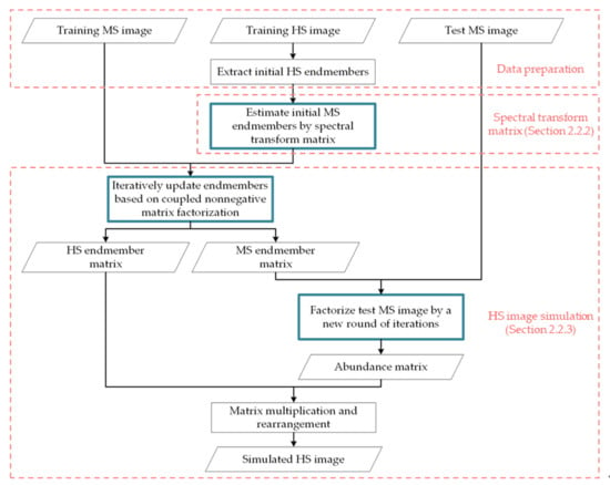
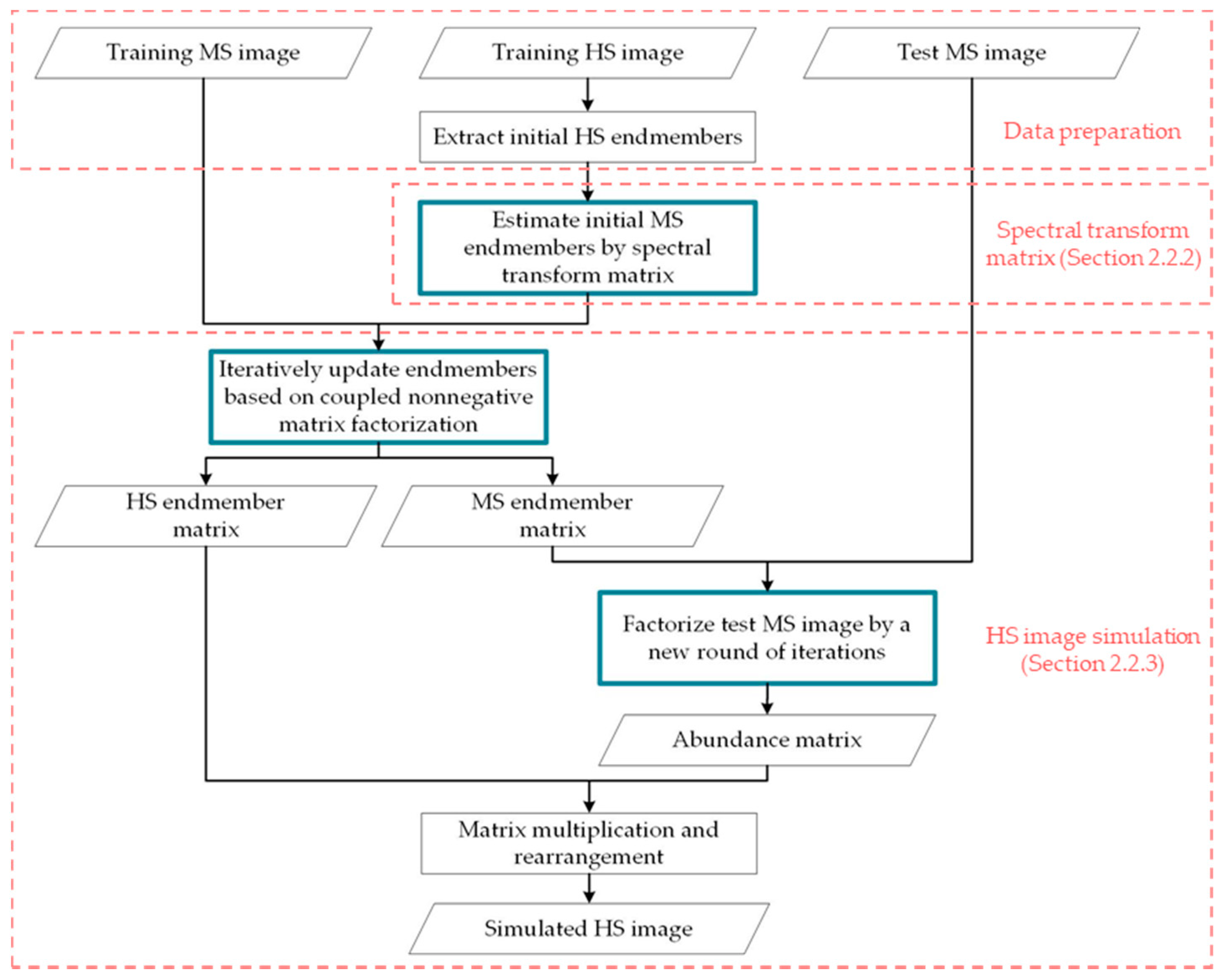
2.2.3. HS Image Simulation and Iterative Calculation Scheme

On the basis of the NMF of images, our approach simulates HS images by multiplying an HS endmember matrix and the abundance matrix of the test MS image.

$$\mathit{H}={\mathit{E}}_H{\mathit{C}}_M+\mathit{N},$$

(9)

where $\mathit{H}\in {ℝ}^{h\times L}$ is the simulated HS image, ${\mathit{E}}_H\in {ℝ}^{h\times n}$ is the HS endmember matrix, and ${\mathit{C}}_M\in {ℝ}^{n\times L}$ is the abundance matrix. To achieve an ideal result, we need to minimize the residual error $\mathit{N}$. We build a cost function $\Vert \mathit{H}-{\mathit{E}}_H{\mathit{C}}_M{\Vert }_F^2$. ${\mathit{E}}_H$ and ${\mathit{C}}_M$, which can minimize the cost function, are our ideal results. However, the simulated image $\mathit{H}$ is unknown and unavailable in solving this function. Then, we use training HS and MS images to compute the accurate ${\mathit{E}}_H$ and ${\mathit{C}}_M$.

In our approach, the training HS image is already prepared in the spectral transformation matrix estimation. We assume that the endmembers, which can properly unmix the training HS data, are also suitable for the global simulated HS image. Therefore, the required endmembers can minimize the residuals in the factorizations of the training HS and MS images. We express these residual minimization as cost functions $\Vert u_h-{\mathit{E}}_h{\mathit{C}}_h{\Vert }_F^2$ and $\Vert u_m-{\mathit{E}}_m{\mathit{C}}_m{\Vert }_F^2$, where $u_h\in {ℝ}^{h\times L}$ and $u_m\in {ℝ}^{m\times L}$ are the overlapped training HS and MS images. As $u_h$ and $u_m$ are factorized by endmembers from the same materials, their abundance matrix should be equal. Meanwhile, the HS and MS endmembers are from the same group of materials. The MS endmembers can be considered as degraded HS endmembers

$${\mathit{E}}_m\approx \mathit{W}{\mathit{E}}_h,$$

(10)

where $\mathit{W}$ is the spectral transformation matrix estimated in Section 2.2.2. To obtain the endmembers that minimize the residuals, we use multiplicative update rules in our simulation approach. The multiplicative update rules, which were proposed by Lee et al., can converge to the local optimal solution under the nonnegativity constraints of two factorized matrixes [29,40]. Yokoya et al. developed a coupled NMF method, which achieves the accurate endmember and abundance matrixes of the test images, on the basis of the multiplicative update rules [32].

Initially, we use vertex component analysis to extract HS endmembers from the training HS image [41]. The number of endmembers is manually set as $n$. The extracted HS endmembers are arranged as the endmember matrix ${\mathit{E}}_h$ of the training HS image. The abundance matrix ${\mathit{C}}_h$ of the training HS image is initialized as $1/n$. Subsequently, we use two rounds of iterative computations to optimize the matrixes of training HS and MS images. In the first round, we fix ${\mathit{E}}_h$. ${\mathit{C}}_h$ is updated using the iterative computation in Equation (11) until the convergence. In the implementation, to avoid excessive computation, the iterative times of Equation (11) is set to no larger than $I_1$, namely, the inner iteration times. The updated ${\mathit{C}}_h$ and initial ${\mathit{E}}_h$ are then alternately optimized by Equations (11) and (12). The iterative calculation is terminated when ${\mathit{E}}_h$ and ${\mathit{C}}_h$ stabilize. In the implementation, the iterative times of Equations (11) and (12) are also limited to no larger than $I_1$. In the second round, we use iterative computations to achieve ${\mathit{E}}_m$ and ${\mathit{C}}_m$. The MS endmember matrix ${\mathit{E}}_m$ is initialized by degrading ${\mathit{E}}_h$ using Equation (10). The initial abundance matrix ${\mathit{C}}_m$ of the training MS image is equal to ${\mathit{C}}_h$. ${\mathit{C}}_m$ is updated by Equation (13) with fixed ${\mathit{E}}_m$. The updated ${\mathit{C}}_m$ and initial ${\mathit{E}}_m$ are then alternately optimized by Equations (13) and (14). Both iterative computations are ended with the convergence. In the implementation, the maximum iteration times in these two computations are set to $I_1$. Afterward, we repeat the above two rounds of computations as global optimization to obtain the optimal ${\mathit{E}}_h$ and ${\mathit{E}}_m$. In the first round of repetitions, initial ${\mathit{C}}_h$ is set equal to the updated ${\mathit{C}}_m$ of Equation (13) in the last iteration. ${\mathit{E}}_h$ is updated by Equation (11) with fixed ${\mathit{C}}_h$. The following alternate updates of ${\mathit{E}}_h$ and ${\mathit{C}}_h$ are the same as above. The maximum repeat times of the two rounds are set as $I_2$, namely, the outer iteration times.

$${\mathit{C}}_h={\mathit{C}}_h\odot \left({\mathit{E}}_h^T{u}_h\right)\oslash \left({\mathit{E}}_h^T{\mathit{E}}_h{\mathit{C}}_h\right),$$

(11)

$${\mathit{E}}_h={\mathit{E}}_h\odot \left(u_h{\mathit{C}}_h^T\right)\oslash \left({\mathit{E}}_h{\mathit{C}}_h{\mathit{C}}_h^T\right),$$

(12)

$${\mathit{C}}_m={\mathit{C}}_m\odot \left({\mathit{E}}_m^T{u}_m\right)\oslash \left({\mathit{E}}_m^T{\mathit{E}}_m{\mathit{C}}_m\right),$$

(13)

$${\mathit{E}}_m={\mathit{E}}_m\odot \left(u_m{\mathit{C}}_m^T\right)\oslash \left({\mathit{E}}_m{\mathit{C}}_m{\mathit{C}}_m^T\right).$$

(14)

where $\odot$ denotes the Hadamard product of matrices [42]. Each element (i, j) in Hadamard product is the product of the elements (i, j) of the original two matrices. $\oslash$ denotes the Hadamard division, which represents the quotient of the corresponding elements in original matrices [43].

After the endmember matrixes ${\mathit{E}}_m$ and ${\mathit{E}}_h$ are obtained, we need to compute the abundance matrix ${\mathit{C}}_M$ of the large-area test MS image. ${\mathit{C}}_M$ is initialized as $1/n$. Then, we use the iterative scheme of Equation (15) to optimize ${\mathit{C}}_M$:

$${\mathit{C}}_M={\mathit{C}}_M\odot \left({\mathit{E}}_m^T\mathit{M}\right)\oslash \left({\mathit{E}}_m^T{\mathit{E}}_m{\mathit{C}}_M\right),$$

(15)

where $\mathit{M}$ denotes the rearranged test MS image and ${\mathit{C}}_M$ is the output when it is convergent. In the implementation, the iteration times of Equation (15) is also limited by $I_1$. Finally, we produce the simulated HS image by

$$\mathit{H}={\mathit{E}}_h{\mathit{C}}_M.$$

(16)

3. Results

In this section, we initially introduce our evaluation protocol of the image simulation. Then, the experimental results and discussions are provided. We compare the spatial and spectral qualities of our method, the PHITA [5], Liu’s method [19], and Chen’s method [18].

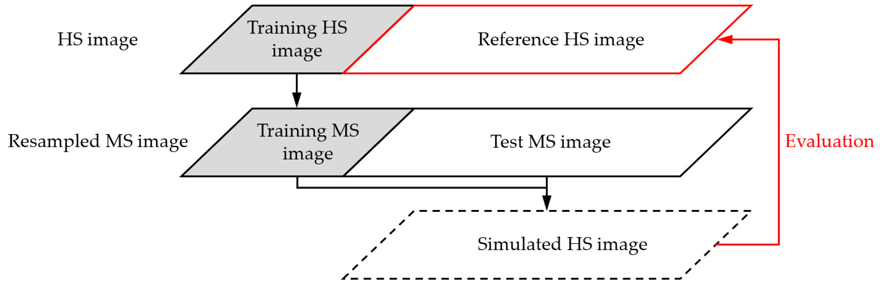
3.1. Evaluation and Comparative Methods

The quality assessment of the simulated HS images is important in the experiments. To use a real HS image as reference, we evaluate the simulated results by referring to the evaluation protocol of the image pansharpening [44]. Figure 4 shows the evaluation flow. Initially, we prepare MS and HS images in the same location. The MS image is resampled to the spatial resolution of the HS image. Then, we extract the overlapped areas in the two images as experiment data. To train the proposed method, we select a subarea in the MS image and the corresponding part in the HS image as the training MS and HS images, respectively. The remaining MS image is used as the test MS image to simulate the HS image. For methods without training data, the HS image is directly produced using the test MS image. Afterward, the remaining HS image is regarded as the reference with ideal quality. The HS images simulated by different approaches are compared with the reference image to assess their qualities objectively.

The quality assessment of the simulated HS images primarily focuses on the visual appearance and quantitative evaluation. The visual appearance provides a general idea of the results. The quantitative evaluation provides fine and objective comparisons. The evaluation indices in our experiments include spectral angle mapper (SAM) [45], RMSE [46], relative dimensionless global error in synthesis (ERGAS) [47], correlation coefficient (CC) [44], universal image quality index (UIQI) [48], adaptive cosine/coherent estimator (ACE) [49,50].

3.2. Experimental Results

The proposed HS image simulation method is compared with PHITA [5], Liu’s method [19], and Chen’s method [18]. All the simulation methods are realized by programing in MATLAB. In the experiments, we test the four methods on each dataset. Figure 5, Figure 6, Figure 7 and Figure 8 present the result images of the four datasets, respectively. As the test datasets have long and narrow shapes, the images presented in these figures are parts of the results.

Table 2. Evaluation results of CIEDE2000.

Datasets	Proposed Method	Chen	UPDM(Liu)	PHITA
1	1.19	6.50	5.02	1.29
2	1.22	15.77	4.28	1.31
3	0.91	7.45	2.24	0.89
4	1.51	6.79	7.71	1.85
Mean	1.21	9.12	4.81	1.34

provides the color qualities of the result images.

Table 3. Quantitative evaluations of datasets.

Datasets	Method	SAM	ERGAS	RMSE	CC	UIQI	ACE
1	Proposed	6.683	16.542	328.4	0.965	0.915	0.21
	Chen	12.911	48.459	1069.1	0.858	0.708	0.08
	UPDM	8.962	68.803	993.4	0.957	0.742	0.07
	PHITA	7.082	17.439	338.1	0.963	0.913	0.19
2	Proposed	3.450	13.348	142.1	0.891	0.841	0.14
	Chen	13.013	45.608	1641.7	0.498	0.350	0.11
	UPDM	13.802	78.619	440.9	0.875	0.709	0.11
	PHITA	3.196	13.310	142.8	0.886	0.834	0.13
3	Proposed	4.791	12.167	191.3	0.972	0.926	0.22
	Chen	15.132	60.631	1609.4	0.736	0.425	0.07
	UPDM	7.083	15.412	266.8	0.968	0.912	0.08
	PHITA	4.818	12.881	196.8	0.969	0.923	0.21
4	Proposed	9.02	25.21	476.9	0.795	0.688	0.09
	Chen	17.466	42.564	1787.5	0.642	0.455	0.07
	UPDM	13.833	65.187	1239.5	0.783	0.607	0.06
	PHITA	10.347	26.521	495.7	0.788	0.695	0.08
Mean	Proposed	5.986	16.817	284.6	0.905	0.842	0.165
	Chen	14.63	49.315	1526.9	0.683	0.484	0.082
	UPDM	10.92	57.005	735.1	0.896	0.742	0.08
	PHITA	6.360	17.538	293.4	0.901	0.841	0.152
Std	Proposed	2.094	5.103	130.3	0.071	0.095	0.053
	Chen	1.861	6.857	272.7	0.131	0.134	0.016
	UPDM	2.972	24.511	395.9	0.074	0.110	0.019
	PHITA	2.683	5.483	136.9	0.073	0.091	0.051

show the quantitative evaluations and the statistics of the four datasets, including means and standard deviations (Stds). In this table, the method with the best quantitative performance is represented by a bold font. The key parameters of our method in the experiments are selected by sensitivity analysis, as presented in Section 4.2.

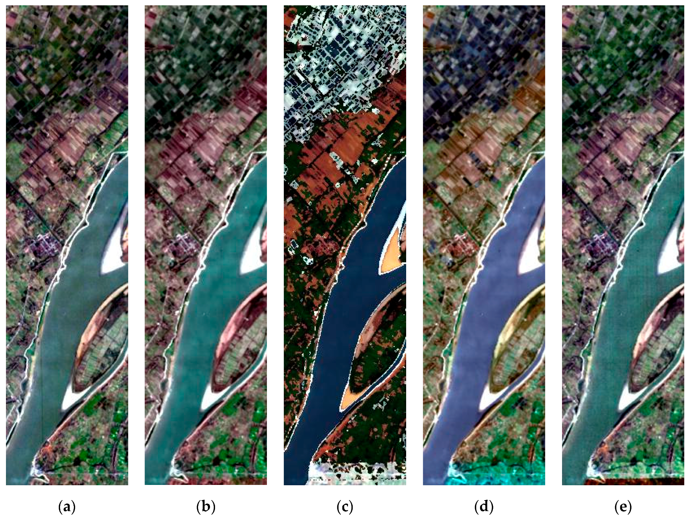
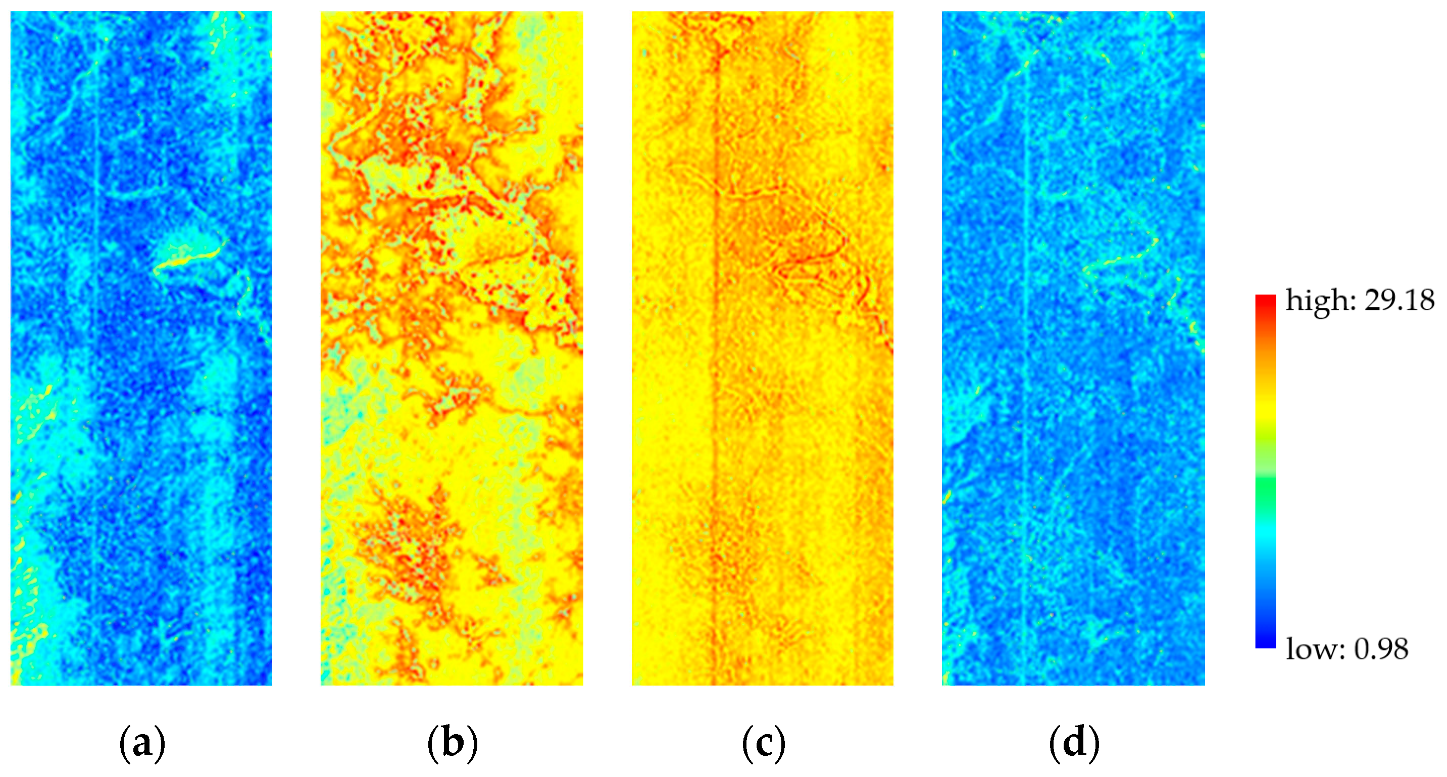
3.2.1. Spatial Performance

We initially compare the simulated images with the reference HS images on the basis of their visual appearance. Figure 5, Figure 7, and Figure 8 present the natural color images of Datasets 1, 3, and 4 (R: 29th band, G: 20th band, B: 12th band), respectively. Figure 6 shows the false color images of Dataset 2 (R: 100th band, G: 75th band, B: 55th band). Each simulation method provides a practicable result. Chen’s method simulates images with larger distortions than the other methods. In Figure 5c, the colors of vegetation and water are considerably different from the reference HS image. In Figure 6c, the spatial details, such as urban area and river, are not efficiently preserved. In Figure 7c and Figure 8c, the farmland is falsely reconstructed with distorted textures and coclors. UPDM provides better visual performance than Chen’s method. The images (d) in Figure 5, Figure 6, Figure 7 and Figure 8 have similar boundaries and textures as the reference HS image. The dense buildings in Figure 5 and the river in Figure 6 are preserved in the results. However, UPDM still produces slight color changes. The colors of vegetation, water, and soil are slightly brighter than those in the reference, as shown in Figure 5, Figure 6 and Figure 8. PHITA and the proposed method provide the two best results. The topographic features and textures of these two results are nearly the and 0.742 (Table 3), respectively, which are higher than those of Chen’s method. The best two results in the comparisons are produced by the proposed method and PHITA. The proposed method achieves the highest CC and UIQI, as shown in Table 3. The highest mean CC (0.905) and UIQI (0.842) in Table 3 reveal that our method generates the best quality spatial information in the four datasets. This quantitative evaluation can also be confirmed by visual appearance. Figure 7b presents similar same as those of the references. The proposed method achieves higher visual quality in Datasets 2 with more realistic colors in water and vegetation than PHITA. We also compute the CIEDE2000 of the RGB bands in each dataset (Table 2). The CIEDE2000 of each method conforms to their visual appearance. The CIEDE2000 of the proposed method is least in most cases (Dataset 1, 2, and 4). PHITA achieves comparable performance. UPDM and Chen’s method rank behind the proposed method and PHITA. In addition, the simulated images provide more clear textures than the reference in Figure 5 and Figure 6. The noises and vertical stripes of the simulated images are also removed in the figures.

The spatial performance of the simulated images is then quantitatively evaluated referring to the real HS image. The main spatial quality evaluation indexes are CC and UIQI in our experiments. Chen’s method achieves the lowest CCs and UIQIs in Table 3. The results are consistent with the geometry and texture information in the mountain area (Figure 5c) and river (Figure 6c). The mean CC and UIQI of Chen’ method are 0.683 and 0.484 (Table 3), respectively, which are worse than those of other methods. UPDM provides more spatial details and less color distortion in the result images, especially in Figure 6d, Figure 7d and Figure 8d, than Chen’s method. The mean CC and UIQI of UPDM are 0.896 edges and colors of the farmland. In Figure 6b, the textures of mountain and urban areas are even clearer than those of the reference. In Figure 8b, most of the spatial information is well generated. PHITA provides comparable results in the figures. In quantitative assessment, the mean CC (0.901) and UIQI (0.841) of PHITA are lower than 0.905 and 0.842, which are achieved by our method.

We further subtract the CCs of UPDM’s results from those of the proposed method’s and PHITA’s results to show the superiority of our method further clearly. As the CCs of Chen’s method are considerably less than those of other methods, we do not present its results. Figure 9 shows the subtraction. A positive value means that the CC performance is better than that of UPDM’s result, whereas a negative value is the opposite. Figure 10 shows the RMSE of each band of PHITA’s and our method’s results. The Figure 9 and Figure 10 confirm that our method has higher qualities than other methods in many bands.

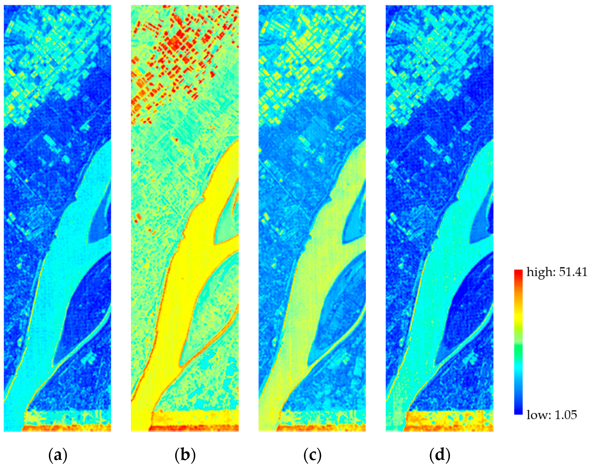
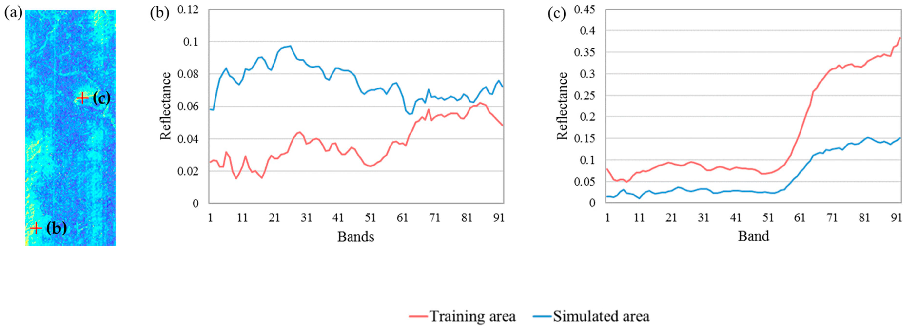
3.2.2. Spectral Performance

We present the SAM distribution images of the Datasets 1–3 in Figure 11, Figure 12 and Figure 13 to visualize the spectral qualities. The pixels with low SAM errors are represented by blue, whereas those with high SAM errors are represented by red. Chen’s method has the most yellow and red pixels in Figure 11, Figure 12 and Figure 13, thereby showing the largest spectral distortion in the comparisons. UPDM produces pixels with large SAM error in global images. For example, Figure 11c consists of light blue and red, indicating that the spectral information of water is not accurately constructed. The images resulted from PHITA have more dark blue pixels and less red pixels, especially in vegetation and water, than those from the other methods. As shown in Figure 11d, the upper mountain area covered by vegetation has minimal SAM error. Therefore, the spectral distortions generated by PHITA are considerably less than those of Chen’s method and UPDM. The proposed method generates a large number of dark blue pixels and little red pixels. Our method constructs more accurate spectrums in vegetation area and water than PHITA. Figure 11a and Figure 12a contain more dark blue area than the other images. In Figure 11a and Figure 13a, the sea and river contain less red and yellow pixels than those of PHITA’s results. Meanwhile, the proposed method produces the least red pixels in Figure 11, which consists of multiple materials and abundant texture features. Thus, our method can reduce spectral distortions in complex areas and has significant advantage in generating high-spectral-quality results.

In quantitative evaluation, the main spectral quality measurements include SAM, ERGAS, RMSE and ACE. Chen’s method provides the poorest spectral quality performance in four datasets (Table 3). UPDM reconstructs a spectrum in each pixel by combining standard spectrums in the library. The mean SAM, ERGAS, RMSE, and ACE of this method are 10.92, 57.005, 735.1, and 0.08 (Table 3), respectively, which are all better than those of Chen’s method. PHITA obtains good spectral qualities in experiments. In Datasets 1, 3, and 4, the spectral indexes of PHITA are all better than those of Chen’s method and UPDM. In Dataset 2, the SAM and ERGAS of PHITA are 3.196 and 13.310, respectively, which are the best in the comparison. The best overall spectral quality on the four datasets is achieved by the proposed method. The mean SAM (5.986), ERGAS (16.817), RMSE (284.6), and ACE (0.165) of our method rank first in Table 3. The best ACE performances are achieved by our method, which demonstrates that our method could preserve subpixel signatures better. The spectral quality of our method is slightly worse than that of PHITA in Dataset 2. The reason is that some of the spectrums in the simulated area are different from the spectrums of the same classes in the training area. The spectral endmembers are extracted from the training area. When we use endmembers to reconstruct these special spectrums, large errors may be obtained. For instance, we present the vegetation and water spectrums of the training and simulated areas in Figure 14. The spectral features of water in training and simulated areas are considerably different, such as the 1st–25th and 40th–60th bands. In Figure 14c, the reflectance values of water in the simulated area are considerably less than those in the training area. Therefore, these special spectrums are constructed with large errors, which reduce the global spectral quality on Dataset 2. In Dataset 4, the spectral qualities of our method and PHITA are a little worse than the other three datasets. The reason is that when the distance between the training and test areas is large, the difference between the spectral information in the two images will increases. Thus, error in the simulation image may be increased. However, if the distance is not too large, the error can be accepted.

3.2.3. Overall Quality

Chen’s method loses considerable spatial details and produces large spectral distortions in the results. UPDM ranks third among the compared methods. This method constructs detailed textures and geometric information but still leads to spectral distortions. PHITA provides good spectral and spatial qualities but is worse than our method in quantitative evaluations. The proposed method achieves the best performance in the global evaluation (Table 3). The advantages of the proposed method are presented as follows:

• The proposed method builds the spectral relation between the MS and HS bands in the same wavelength ranges. The simulated images can be generated by using prior HS endmembers extracted from training HS images. In this manner, the relations between the bands of spectral endmembers are preserved, and fine spectral features are achieved in the simulated images.
• The proposed method reconstructs the simulated images by combining the spectrums of related materials, pixel by pixel. Following this strategy, the simulation of each pixel is independent, which can improve the spectral quality of the areas with complex materials and objects.
• We utilize iterative schemes to optimize the endmembers and abundance matrixes of the images. This method reduces the residual error in unmixing and reconstruction, thereby further improving the global quality of the results. Our method achieves the best performance in Table 3.

All simulation methods are realized using MATLAB. A laptop computer with a 10 G memory, Intel Core i5 CPU, and Windows 10 system is used for the experiments. The processing time of the proposed method, UPDM, Chen’s method and PHITA are presented in

Table 4. Computational times of simulation methods (second).

Dataset	Proposed Method	Chen	UPDM(Liu)	PHITA
1	151.54	44.49	141.75	30.16
2	47.77	10.24	12.34	8.26
3	121.42	34.18	49.69	28.91
4	57.91	10.47	6.4	5.6
Mean	94.66	24.84	52.55	18.23

. Our method consumes more time than UPDM (52.55.64s), PHITA (18.23s) and Chen’s method (28.84s). However, this limitation can be acceptable in many application fields. The proposed HS image simulation method can provide results with higher spatial and spectral qualities than Chen’s method, UPDM, and PHITA with acceptable efficiency.

4. Discussion

In this section, we discuss the features of our approach. Afterward, a detailed sensitivity analysis is conducted to select the optimal parameters of the four datasets.

4.1. Result Analysis

As shown in Section 3.2, the proposed method achieves better performance than Chen’s method, UPDM, and PHITA in spatial and spectral qualities. The main features of our approach focus on using the prior MS and HS endmembers and independently constructing pixels and the iteration schemes based on multiplicative update rules.

The proposed method uses the endmembers extracted from training images in HS image simulation. The pixels are produced by the prior spectral information of the similar materials. Following this strategy, all bands in a pixel are constructed simultaneously by the same endmembers and coefficients. Therefore, the fine spectral features of the materials can be efficiently restored. PHITA utilizes different MS bands and linear coefficients to produce each HS band independently. The relations between the simulated bands may be not well considered, which easily leads to spectral distortions in the result. In addition, the proposed method achieves better performance in high spatial resolution image. The reason may be the images with high spatial resolution contain more pure pixels, which can be simulated easily.

For the areas with complex and multi-class objects, the HS image simulation may suffer from large errors because of the various spectral features and high heterogeneity. Our method produces HS images pixel by pixel. Thus, each pixel is generated independently and is slightly influenced by the neighboring pixels and environment. The pixels with special spectral information or textures can be efficiently processed through our method. Chen’s method provides the results by classifying the test MS image and replacing the MS information. In this method, the pixels in complex areas are easily misclassified. Consequently, the spectral and spatial qualities of the results will be significantly reduced.

The iteration schemes of our method can effectively optimize the HS and MS endmembers. After alternately updating, the spectral endmembers factorize the images with less residuals, indicating that the endmembers can compose most of the spectrums in the images. Thus, the spectral endmembers become further suitable for the training and test images after our iteration schemes. Then, the accuracy of the results can be improved. UPDM simulated images are also based on spectral unmixing. However, the standard spectrums are often different from the actual spectrums in the study area, which easily leads to large residuals in pixel unmixing. The large residuals of UPDM reduce the quality of the result.

4.2. Sensitivity Analysis

In the proposed method, the accuracy of the simulated images is significantly influenced by the parameters, including the inner iteration times $I_1$, the outer iteration times $I_2$, and the number of spectral endmembers $n$. To find appropriate parameters of the proposed method, we initially provide a detailed parameter analysis on Dataset 1. Then, the parameters of other datasets are selected by fine-tuning those of Dataset 1. In addition, finding the optimal parameters needs testing all the parameters by lots of experiments. The number of experiments in this section could not ensure that the selected parameters are optimal. The parameters we provided is just suitable for the test datasets.

4.2.1. Iteration Times

The optimal endmember and abundance matrixes are obtained through iterative calculation. When the iteration times are increasing, the factorized matrixes of images will be gradually optimized. Therefore, we must find suitable times for obtaining optimal results with low computational cost. The iterative times in our method include $I_1$ and $I_2$. $I_1$ is the iteration time of each equation. $I_2$ is the repeat time of the two rounds of computations. Figure 15 presents the quantitative results with different iteration times. When $I_1$ is larger than 250, the evaluation indexes vibrate near stable values. When $I_2$ reaches 5, the evaluation indexes are not continuously improved. Therefore, to achieve the optimal result with less calculation amount, we set $I_1=250$ and $I_2=5$ in the experiment on Dataset 1.

We then extend the obtained iteration parameters to the other datasets by fine tuning. In Dataset 2, the iteration times of our method are set to $I_1=150$ and $I_2=5$. The parameters on Dataset 3 and 4 are both $I_1=250$ and $I_2=5$.

4.2.2. Number of Endmembers

In our approach, a large number of endmembers can provide abundant spectral information, which helps improve the accuracy of the simulated images. However, massive endmembers will not contribute to the quality of the results. Meanwhile, numerous endmembers may increase the computation complexity of our method. Thus, we performed detailed experiments to find the suitable number of endmembers. Figure 16 shows the results. If the number of endmembers is small, then the result HS images have large errors, such as $n=5$. With the increase in $n$, the evaluation indexes are gradually improved. When $n>40$, the result qualities are not continuously increased. Therefore, we set the number of endmembers to 40 in the experiments on Dataset 1.

To find the suitable numbers of endmembers on Datasets 2 and 3, we conduct a detailed analysis. After parameter tuning, the suitable numbers of endmembers on Datasets 2, 3, and 4 are determined as 30, 40, 40, respectively. When an unknown dataset is processed by our method, the initial number of the endmembers is suggested to be about 40. Then, this number can be fine-tuned referring to the result quality and computing time to obtain an appropriate value.

5. Conclusions

In this paper, we propose a novel HS image simulation method based on NMF. Our main contributions are developing the spectral transformation matrix between the HS and MS endmembers and designing the simulation method for constructing the HS image. The spectral transformation matrix is estimated between each MS band and the HS bands in the same wavelength range by using the linear regression model. This matrix helps obtain the corresponding MS and HS endmembers. The proposed method uses iterative computations based on NMF to optimize the extracted endmembers, which are used to simulate the final HS image.

Experiments are performed on four datasets from EO-1 and HJ-1A satellites. Results illustrate that the proposed method can provide simulated images with good spectral and spatial qualities. In comparison with UPDM, PHITA, and Chen’s method, the proposed method has advantages in producing clear textures and reducing spectral distortions in the areas with complex and multi-class objects. The four evaluation indexes, namely, SAM, ERGAS, RMSE, CC, UIQI and ACE, in Table 3 are 5.986, 16.817, 284.6, 0.905, 0.842, and 0.165, respectively, which are better than those of other methods.

However, in our approach, if the spectrums in the simulated HS image are considerably different from the prior endmember of the same material in the training images, then these spectrums are difficult to produce precisely. This case may lead to large errors in the results. In addition, the proposed method consumes more time than other methods. In the future, we will focus on correcting the endmembers referring to the spatial location and corresponding MS information in the simulation of each pixel. The acceleration of our method will also be considered in our future work.

References

1. Pelta, R.; Ben-Dor, E. Assessing the detection limit of petroleum hydrocarbon in soils using hyperspectral remote-sensing. Remote Sens. Environ. 2019, 224, 145–153. [Google Scholar] [CrossRef]
2. Li, N.; Huang, X.; Zhao, H.; Qiu, X.; Deng, K.; Jia, G.; Li, Z.; Fairbairn, D.; Gong, X. A Combined Quantitative Evaluation Model for the Capability of Hyperspectral Imagery for Mineral Mapping. Sensors 2019, 19, 328. [Google Scholar] [CrossRef] [PubMed]
3. Veraverbeke, S.; Dennison, P.; Gitas, I.; Hulley, G.; Kalashnikova, O.; Katagis, T.; Kuai, L.; Meng, R.; Roberts, D.; Stavros, N. Remote Sensing of Environment Hyperspectral remote sensing of fire: State-of-the-art and future perspectives. Remote Sens. Environ. 2018, 216, 105–121. [Google Scholar] [CrossRef]
4. Tan, Y.; Sun, J.; Zhang, B.; Chen, M.; Liu, Y.; Liu, X. Sensitivity of a Ratio Vegetation Index Derived from Hyperspectral Remote Sensing to the Brown Planthopper Stress on Rice Plants. Sensors 2019, 19, 375. [Google Scholar] [CrossRef]
5. Hoang, N.T.; Koike, K. Transformation of Landsat imagery into pseudo-hyperspectral imagery by a multiple regression-based model with application to metal deposit-related minerals mapping. ISPRS J. Photogramm. Remote Sens. 2017, 133, 157–173. [Google Scholar] [CrossRef]
6. Miura, T.; Huete, A.; Yoshioka, H. An empirical investigation of cross-sensor relationships of NDVI and red/near-infrared reflectance using EO-1 Hyperion data. Remote Sens. Environ. 2006, 100, 223–236. [Google Scholar] [CrossRef]
7. USGS Earth Observing 1 (EO-1). Available online: https://archive.usgs.gov/archive/sites/eo1.usgs.gov/index.html (accessed on 21 May 2019).
8. Zhu, X.; Chen, J.; Gao, F.; Chen, X.; Masek, J.G. An enhanced spatial and temporal adaptive reflectance fusion model for complex heterogeneous regions. Remote Sens. Environ. 2010, 114, 2610–2623. [Google Scholar] [CrossRef]
9. Ju, J.; Roy, D.P. The availability of cloud-free Landsat ETM+ data over the conterminous United States and globally. Remote Sens. Environ. 2008, 112, 1196–1211. [Google Scholar] [CrossRef]
10. Sun, X.; Zhang, L.; Yang, H.; Wu, T.; Cen, Y.; Guo, Y. Enhancement of Spectral Resolution for Remotely Sensed Multispectral Image. IEEE J. Sel. Top. Appl. Earth Obs. Remote Sens. 2015, 8, 2198–2211. [Google Scholar] [CrossRef]
11. Immitzer, M.; Vuolo, F.; Atzberger, C. First experience with Sentinel-2 data for crop and tree species classifications in central Europe. Remote Sens. 2016, 8, 166. [Google Scholar] [CrossRef]
12. Dierckx, W.; Sterckx, S.; Benhadj, I.; Livens, S.; Duhoux, G.; Van Achteren, T.; Francois, M.; Mellab, K.; Saint, G. PROBA-V mission for global vegetation monitoring: standard products and image quality. Int. J. Remote Sens. 2014, 35, 2589–2614. [Google Scholar] [CrossRef]
13. Hoan, N.T.; Tateishi, R. Cloud Removal of Optical Image Using SAR Data for ALOS Applications. Experimenting on Simulated ALOS Data. J. Remote Sens. Soc. Japan 2009, 29, 410–417. [Google Scholar]
14. Wulder, M.A.; White, J.C.; Loveland, T.R.; Woodcock, C.E.; Belward, A.S.; Cohen, W.B.; Fosnight, E.A.; Shaw, J.; Masek, J.G.; Roy, D.P. The global Landsat archive: Status, consolidation, and direction. Remote Sens. Environ. 2016, 185, 271–283. [Google Scholar] [CrossRef] [Green Version]
15. Huo, H.; Guo, J.; Li, Z. Hyperspectral Image Classification for Land Cover Based on an Improved Interval Type-II Fuzzy C-Means Approach. Sensors 2018, 18, 363. [Google Scholar] [CrossRef] [PubMed]
16. Song, Y.-Q.; Zhao, X.; Su, H.-Y.; Li, B.; Hu, Y.-M.; Cui, X.-S. Predicting Spatial Variations in Soil Nutrients with Hyperspectral Remote Sensing at Regional Scale. Sensors 2018, 18, 3086. [Google Scholar] [CrossRef] [PubMed]
17. Fan, L.; Zhao, J.; Xu, X.; Liang, D.; Yang, G.; Feng, H.; Yang, H.; Wang, Y.; Chen, G.; Wei, P. Hyperspectral-based Estimation of Leaf Nitrogen Content in Corn Using Optimal Selection of Multiple Spectral Variables. Sensors 2019, 19, 2898. [Google Scholar] [CrossRef]
18. Chen, F.; Niu, Z.; Sun, G.Y.; Wang, C.Y.; Teng, J. Using low-spectral-resolution images to acquire simulated hyperspectral images. Int. J. Remote Sens. 2008, 29, 2963–2980. [Google Scholar] [CrossRef]
19. Liu, B.; Zhang, L.; Zhang, X.; Zhang, B.; Tong, Q. Simulation of EO-1 Hyperion Data from ALI Multispectral Data Based on the Spectral Reconstruction Approach. Sensors 2009, 9, 3090–3108. [Google Scholar] [CrossRef]
20. Winter, M.E.; Winter, E.M.; Beaven, S.G.; Ratkowski, A.J. Hyperspectral image sharpening using multispectral data. In Proceedings of the IEEE Aerospace Conference, Big Sky, MT, USA, 3–10 March 2007; pp. 1–9. [Google Scholar]
21. Winter, M.E.; Winter, E.M.; Beaven, S.G.; Ratkowski, A.J. High-performance fusion of multispectral and hyperspectral data. In Proceedings of the Defense and Security Symposium, Orlando, FL, USA, 17–21 April 2006; Volume 6233. [Google Scholar]
22. Zhang, Z.; Shi, Z. Nonnegative matrix factorization-based hyperspectral and panchromatic image fusion. Neural Comput. Appl. 2013, 23, 895–905. [Google Scholar] [CrossRef]
23. Lin, C.; Ma, F.; Chi, C.; Hsieh, C. A Convex Optimization-Based Coupled Nonnegative Matrix Factorization Algorithm for Hyperspectral and Multispectral Data Fusion. IEEE Trans. Geosci. Remote Sens. 2018, 56, 1652–1667. [Google Scholar] [CrossRef]
24. Zhang, K.; Wang, M.; Yang, S.; Xing, Y.; Qu, R. Fusion of Panchromatic and Multispectral Images via Coupled Sparse Non-Negative Matrix Factorization. IEEE J. Sel. Top. Appl. Earth Obs. Remote Sens. 2016, 9, 5740–5747. [Google Scholar] [CrossRef]
25. Karoui, M.S.; Deville, Y.; Benhalouche, F.Z.; Boukerch, I. Hypersharpening by joint-criterion nonnegative matrix factorization. IEEE Trans. Geosci. Remote Sens. 2016, 55, 1660–1670. [Google Scholar] [CrossRef]
26. Dong, W.; Fu, F.; Shi, G.; Cao, X.; Wu, J.; Li, G.; Li, X. Hyperspectral image super-resolution via non-negative structured sparse representation. IEEE Trans. Image Process. 2016, 25, 2337–2352. [Google Scholar] [CrossRef] [PubMed]
27. Yang, J.; Wright, J.; Huang, T.S.; Ma, Y. Image super-resolution via sparse representation. IEEE Trans. Image Process. 2010, 19, 2861–2873. [Google Scholar] [CrossRef] [PubMed]
28. Nieves, J.L.; Valero, E.M.; Romero, J.; Henández-Andrés, J. Spectral recovery of artificial illuminants using a CCD colour camera with Non-negative Matrix Factorization and Independent Component Analysis. In Proceedings of the Conference on Colour in Graphics, Imaging, and Vision; Society for Imaging Science and Technology, Leeds, UK, 19–22 June 2006; pp. 237–240. [Google Scholar]
29. Liu, X.; Xia, W.; Wang, B.; Zhang, L. An approach based on constrained nonnegative matrix factorization to unmix hyperspectral data. IEEE Trans. Geosci. Remote Sens. 2011, 49, 757–772. [Google Scholar] [CrossRef]
30. Huck, A.; Guillaume, M.; Blanc-Talon, J. Minimum dispersion constrained nonnegative matrix factorization to unmix hyperspectral data. IEEE Trans. Geosci. Remote Sens. 2010, 48, 2590–2602. [Google Scholar] [CrossRef]
31. Jia, S.; Qian, Y. Constrained nonnegative matrix factorization for hyperspectral unmixing. IEEE Trans. Geosci. Remote Sens. 2008, 47, 161–173. [Google Scholar] [CrossRef]
32. Yokoya, N.; Yairi, T.; Iwasaki, A. Coupled nonnegative matrix factorization unmixing for hyperspectral and multispectral data fusion. IEEE Trans. Geosci. Remote Sens. 2012, 50, 528–537. [Google Scholar] [CrossRef]
33. Poovalinga Ganesh, B.; Aravindan, S.; Raja, S.; Thirunavukkarasu, A. Hyperspectral satellite data (Hyperion) preprocessing—a case study on banded magnetite quartzite in Godumalai Hill, Salem, Tamil Nadu, India. Arab. J. Geosci. 2012, 6, 3249–3256. [Google Scholar] [CrossRef]
34. Datt, B.; Mcvicar, T.; Van Niel, T.; L B Jupp, D.; Pearlman, J. Preprocessing EO-1 Hyperion hyperspectral data to support the application of agricultural indexes. IEEE Trans. Geosci. Remote Sens. 2003, 41, 1246–1259. [Google Scholar] [CrossRef]
35. Shi, C.; Wang, L. Incorporating spatial information in spectral unmixing: A review. Remote Sens. Environ. 2014, 149, 70–87. [Google Scholar] [CrossRef]
36. Heylen, R.; Parente, M.; Member, S.; Gader, P. review of nonlinear HS-unmixing methods. IEEE Trans. Geosci. Remote Sens. 2014, 7, 1844–1868. [Google Scholar]
37. Heylen, R.; Scheunders, P. A multilinear mixing model for nonlinear spectral unmixing. IEEE Trans. Geosci. Remote Sens. 2016, 54, 240–251. [Google Scholar] [CrossRef]
38. Hoang, N.T.; Koike, K. Comparison of hyperspectral transformation accuracies of multispectral Landsat TM, ETM+, OLI and EO-1 ALI images for detecting minerals in a geothermal prospect area. ISPRS J. Photogramm. Remote Sens. 2018, 137, 15–28. [Google Scholar] [CrossRef]
39. China Centre for Resource Satellite Data and Application. Available online: http://www.cresda.com/n16/ (accessed on 2 November 2018).
40. Lee, D.D.; Seung, H.S. Learning the parts of objects by non-negative matrix factorization. Nature 1999, 401, 788–791. [Google Scholar] [CrossRef]
41. Nascimento, J.M.P.; Dias, J.M.B. Vertex component analysis: A fast algorithm to unmix hyperspectral data. IEEE Trans. Geosci. Remote Sens. 2005, 43, 898–910. [Google Scholar] [CrossRef]
42. Styan, G.P.H. Hadamard products and multivariate statistical analysis. Linear Algebra Appl. 1973, 6, 217–240. [Google Scholar] [CrossRef] [Green Version]
43. Wetzstein, G.; Lanman, D.; Hirsch, M.; Raskar, R. Tensor Displays: Compressive Light Field Synthesis Using Multilayer Displays with Directional Backlighting. 2012. Available online: http://hdl.handle.net/1721.1/92408 (accessed on 17 October 2019).
44. Loncan, L.; De Almeida, L.B.; Bioucas-Dias, J.M.; Briottet, X.; Chanussot, J.; Dobigeon, N.; Fabre, S.; Liao, W.; Licciardi, G.A.; Simoes, M.; et al. Hyperspectral Pansharpening: A Review. IEEE Geosci. Remote Sens. Mag. 2015, 3, 27–46. [Google Scholar] [CrossRef] [Green Version]
45. Kruse, F.A.; Lefkoff, A.B.; Boardman, J.W.; Heidebrecht, K.B.; Shapiro, A.T.; Barloon, P.J.; Goetz, A.F.H. The spectral image processing system (SIPS)—interactive visualization and analysis of imaging spectrometer data. Remote Sens. Environ. 1993, 44, 145–163. [Google Scholar] [CrossRef]
46. Aiazzi, B.; Alparone, L.; Baronti, S.; Garzelli, A.; Selva, M. Twenty-five years of pansharpening: A critical review and new developments. In Signal and Image Processing for Remote Sensing; CRC Press: Boca Raton, FL, USA, 2012; pp. 552–599. [Google Scholar]
47. Wald, L. Quality of high resolution synthesised images: Is there a simple criterion? In Proceedings of the SEE/URISCA Third conference “Fusion of Earth data: merging point measurements, raster maps and remotely sensed images”, Sophia Antipolis, France, 26–28 January 2000; pp. 99–103. [Google Scholar]
48. Wang, Z.; Bovik, A.C. A universal image quality index. IEEE Signal Process. Lett. 2002, 9, 81–84. [Google Scholar] [CrossRef]
49. Sidike, P.; Asari, V.K.; Alam, M.S. Multiclass object detection with single query in hyperspectral imagery using class-associative spectral fringe-adjusted joint transform correlation. IEEE Trans. Geosci. Remote Sens. 2015, 54, 1196–1208. [Google Scholar] [CrossRef]
50. Broadwater, J.; Chellappa, R. Hybrid detectors for subpixel targets. IEEE Trans. Pattern Anal. Mach. Intell. 2007, 29, 1891–1903. [Google Scholar] [CrossRef] [PubMed]
Figure 1. Geographic locations of the ALI and Hyperion images in Dataset 4.
Remotesensing 11 02416 g001
Figure 2. Comparison between the wavelength ranges of the bands: (a) Hyperion (HS) and ALI (MS) data, (b) HSI (HS) and CCD (MS) data.
Remotesensing 11 02416 g002
Figure 3. Overview of our HS image simulation approach.
Remotesensing 11 02416 g003
Figure 4. The evaluation flow of the HS image simulation.
Remotesensing 11 02416 g004
Figure 5. The reference and simulated HS images of dataset 1 (R: 29th band, G: 20th band, B: 12th band): (a) reference HS image, (b) proposed method, (c) Chen, (d) UPDM, (e) PHITA.
Remotesensing 11 02416 g005
Figure 6. The reference and simulated HS images of dataset 2 (R: 100th band, G: 75th band, B: 55th band): (a) reference HS image, (b) proposed method, (c) Chen, (d) UPDM, (e) PHITA.
Remotesensing 11 02416 g006
Figure 7. The reference and simulated HS images of dataset 3 (R: 29th band, G: 20th band, B: 12th band): (a) reference HS image, (b) proposed method, (c) Chen, (d) UPDM, (e) PHITA.
Remotesensing 11 02416 g007
Figure 8. The reference and simulated HS images of dataset 4 (R: 29th band, G: 20th band, B: 12th band): (a) reference HS image, (b) proposed method, (c) Chen, (d) UPDM, (e) PHITA.
Remotesensing 11 02416 g008
Figure 9. Subtractions of CCs of UPDM’s results from CCs of the proposed method’s and PHITA’s results in all bands: (a) Dataset 1, (b) Dataset 3.
Remotesensing 11 02416 g009
Figure 10. RMSE of the proposed method’s and PHITA’s results in all bands: (a) Dataset 1, (b) Dataset 3 (The 1st band in the figure is the 10th band in original HS data).
Remotesensing 11 02416 g010
Figure 11. SAM distribution image of dataset 1: (a) proposed method, (b) Chen, (c) UPDM, (d) PHITA.
Remotesensing 11 02416 g011
Figure 12. SAM distribution image of dataset 2: (a) proposed method, (b) Chen, (c) UPDM, (d) PHITA.
Remotesensing 11 02416 g012
Figure 13. SAM distribution image of dataset 3: (a) proposed method, (b) Chen, (c) UPDM, (d) PHITA.
Remotesensing 11 02416 g013
Figure 14. Spectrums in Dataset 2: (a) SAM distribution image of the proposed method on Dataset 2, (b) spectrums of vegetation in training area and simulated area, (c) spectrums of water in training area and simulated area.
Remotesensing 11 02416 g014
Figure 15. The influence of iteration times I 1 and I 2 on the result image: (a) SAM, (b) RMSE, (c) CC, (d) UIQI.
Remotesensing 11 02416 g015
Figure 16. The influence of the number of endmembers on the result image: (a) SAM, (b) RMSE, (c) CC, (d) UIQI.
Remotesensing 11 02416 g016