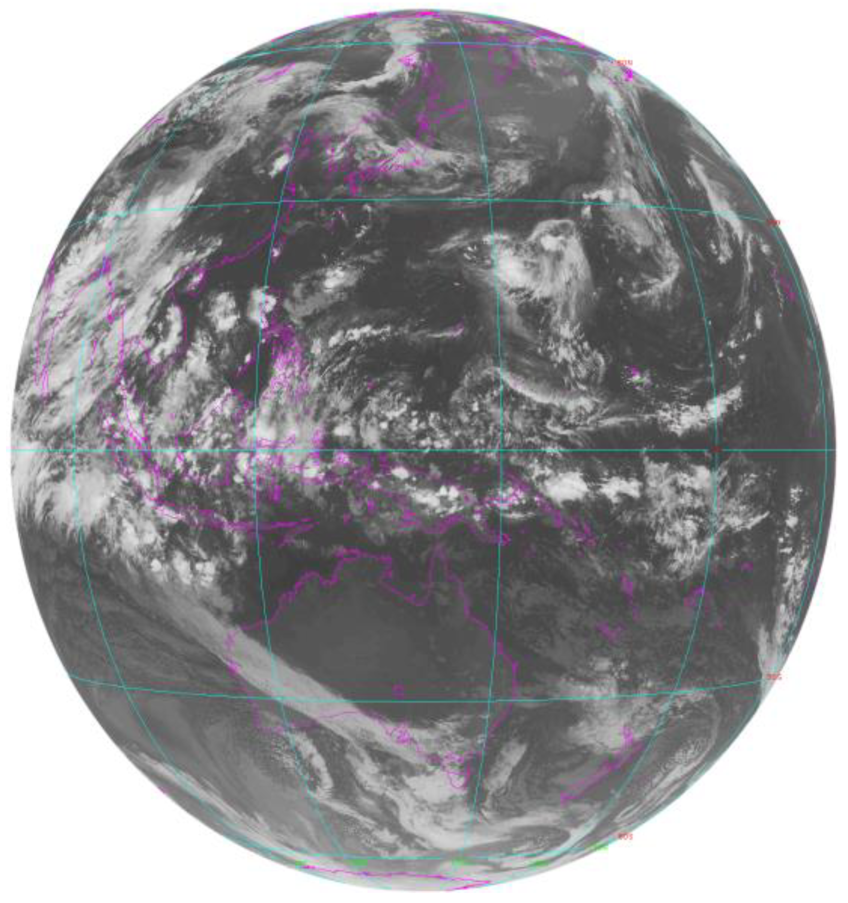
Figure 1.
Himawari-8 10.4 µm satellite image for 21 July 2016 at 1200 UTC.
Figure 1.
Himawari-8 10.4 µm satellite image for 21 July 2016 at 1200 UTC.
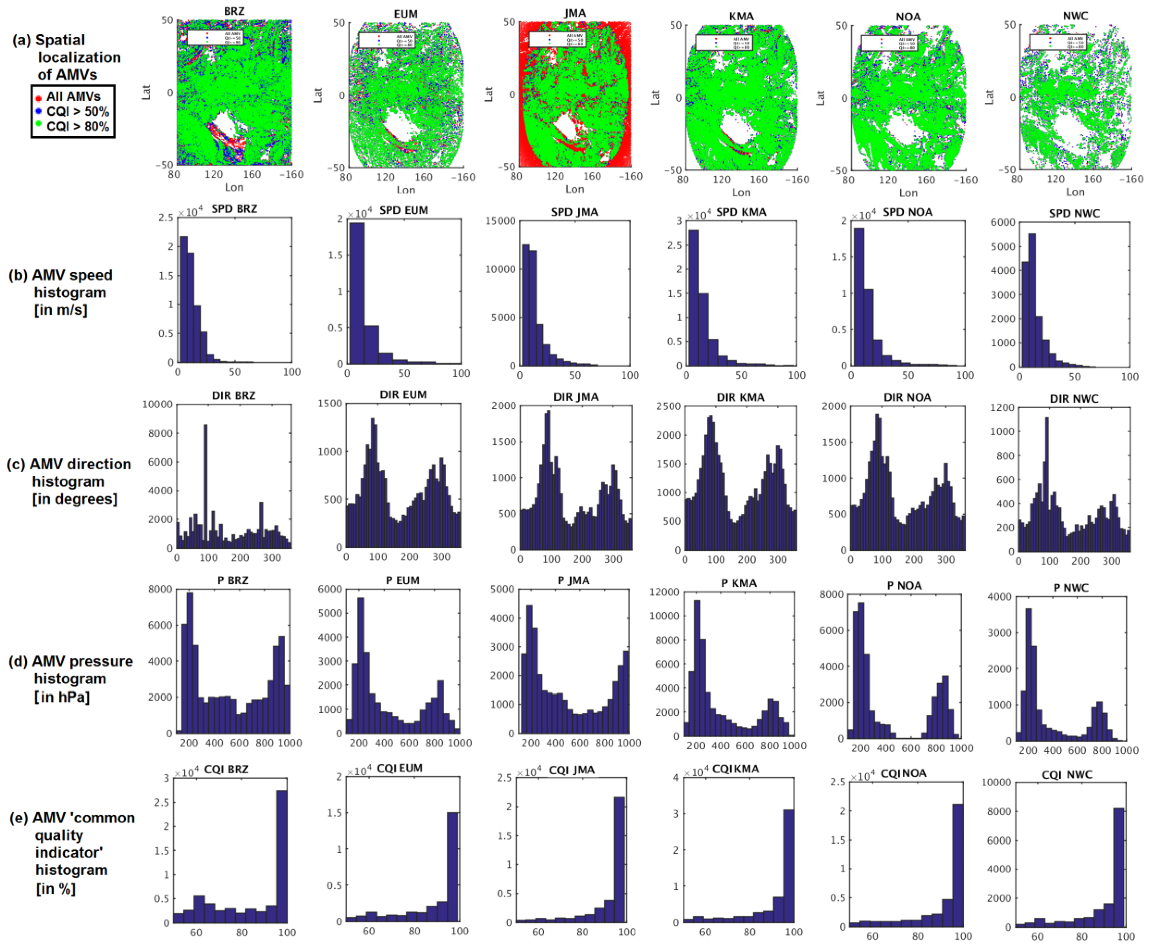
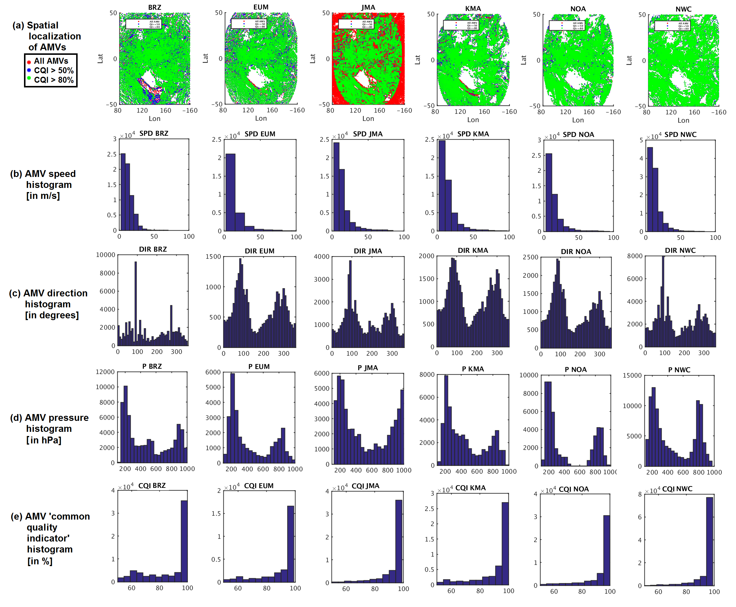
Figure 2.
Spatial localization of Atmospheric Motion Vectors (AMVs) (a), and histograms of parameters: (b) AMV speed in m s−1, (c) AMV direction in degrees, (d) AMV pressure in hPa, (e) AMV CQI (Common Quality Indicator) in %, for the AMV datasets in Experiment 1 with CQI >= 50%. From left to right, BRZ, EUM, JMA, KMA, NOA, NWC. BRZ: Brazil Center for Weather Prediction and Climate Studies (CPTEC/INPE); EUM: European Organization for the Exploitation of Meteorological Satellites (EUMETSAT); JMA: Japan Meteorological Agency; KMA: Korea Meteorological Administration; NOA: United States National Oceanic and Atmospheric Administration (NOAA); NWC: Satellite Application Facility on Support to Nowcasting (NWCSAF).
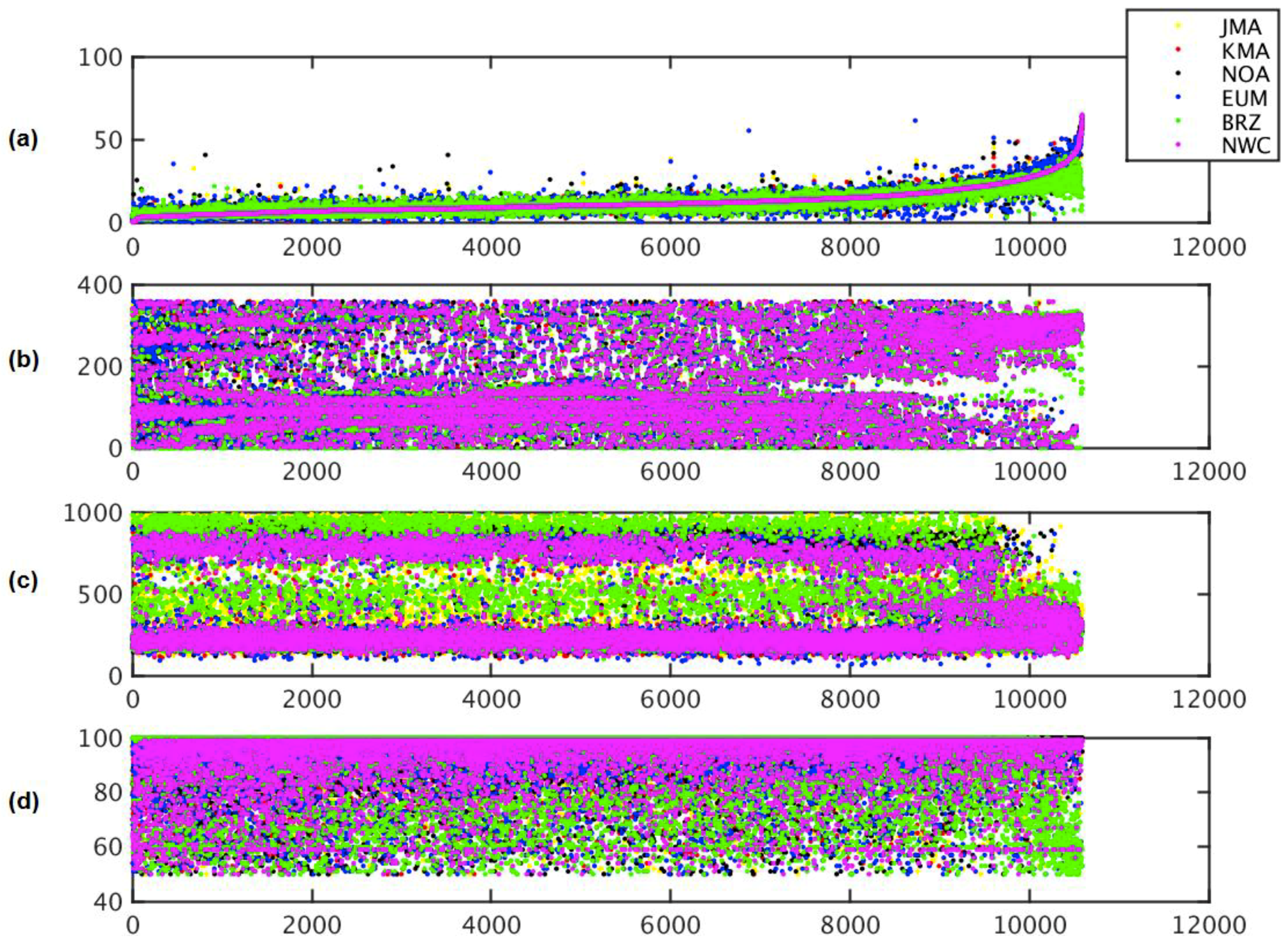
Figure 3.
‘Parameter plot’ for collocated AMVs from the different AMV datasets in Experiment 1, with CQI >= 50% and a collocation distance up to 55 km. Considered variables are speed (a), direction (b), pressure (c), and CQI (d). Color codes correspond to BRZ in green, EUM in blue, JMA in yellow, KMA in red, NOA in black, NWC in magenta.
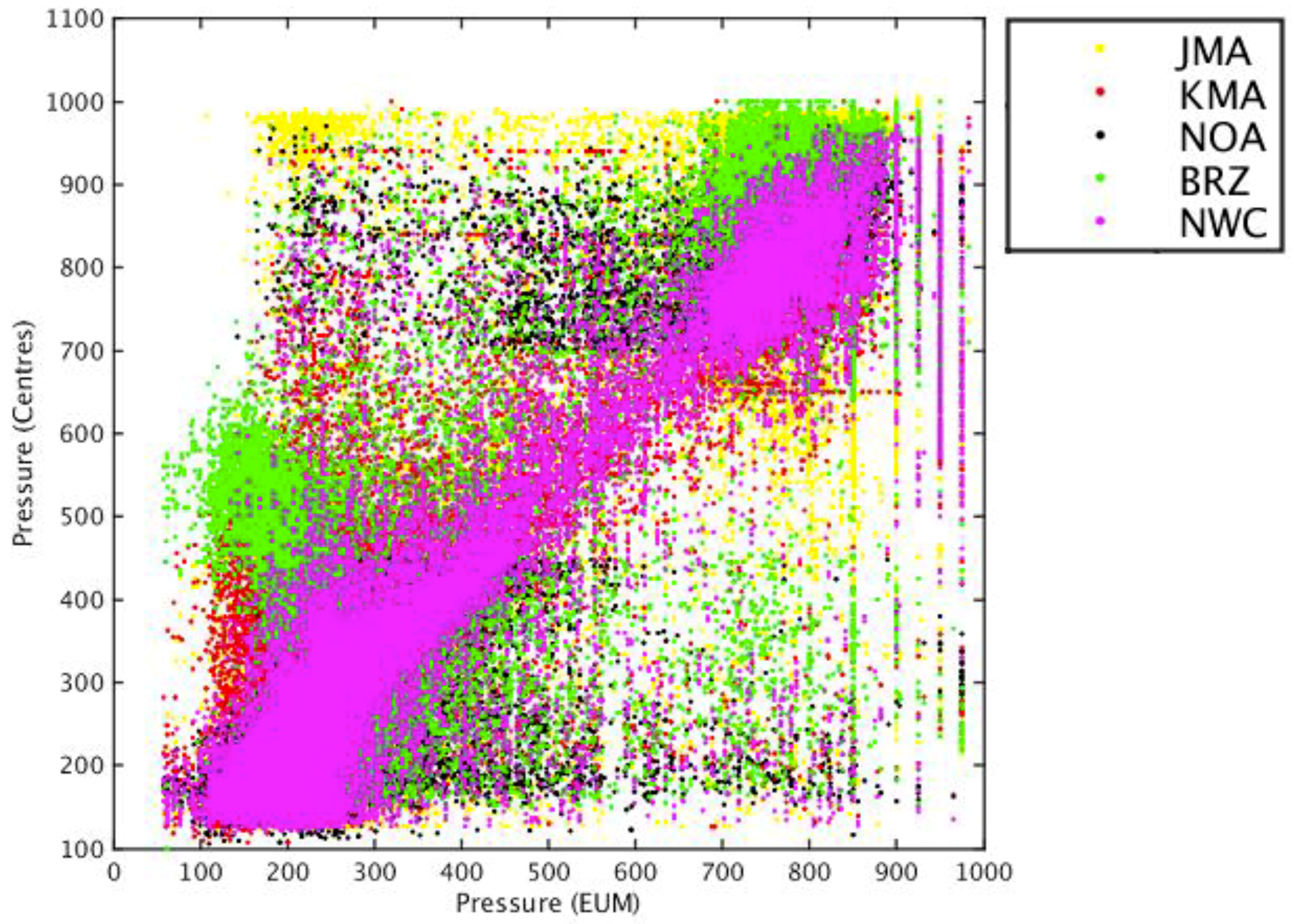
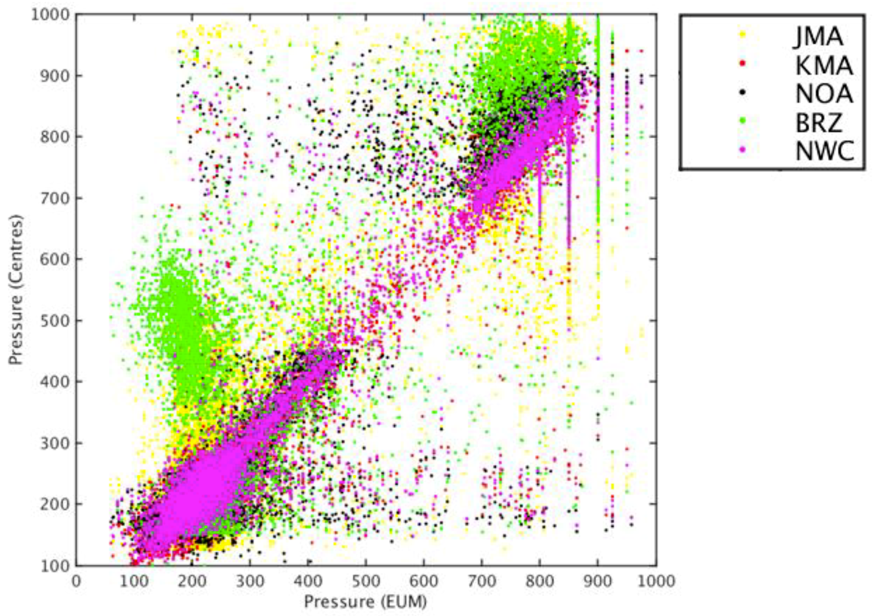
Figure 4.
Scatterplot of collocated AMV pressures for Experiment 1, using CQI >= 50% and a collocation distance up to 55 km, for each center versus EUM AMV pressures (BRZ in green; JMA in yellow; KMA in red; NOA in black; NWC in magenta).
Figure 4.
Scatterplot of collocated AMV pressures for Experiment 1, using CQI >= 50% and a collocation distance up to 55 km, for each center versus EUM AMV pressures (BRZ in green; JMA in yellow; KMA in red; NOA in black; NWC in magenta).
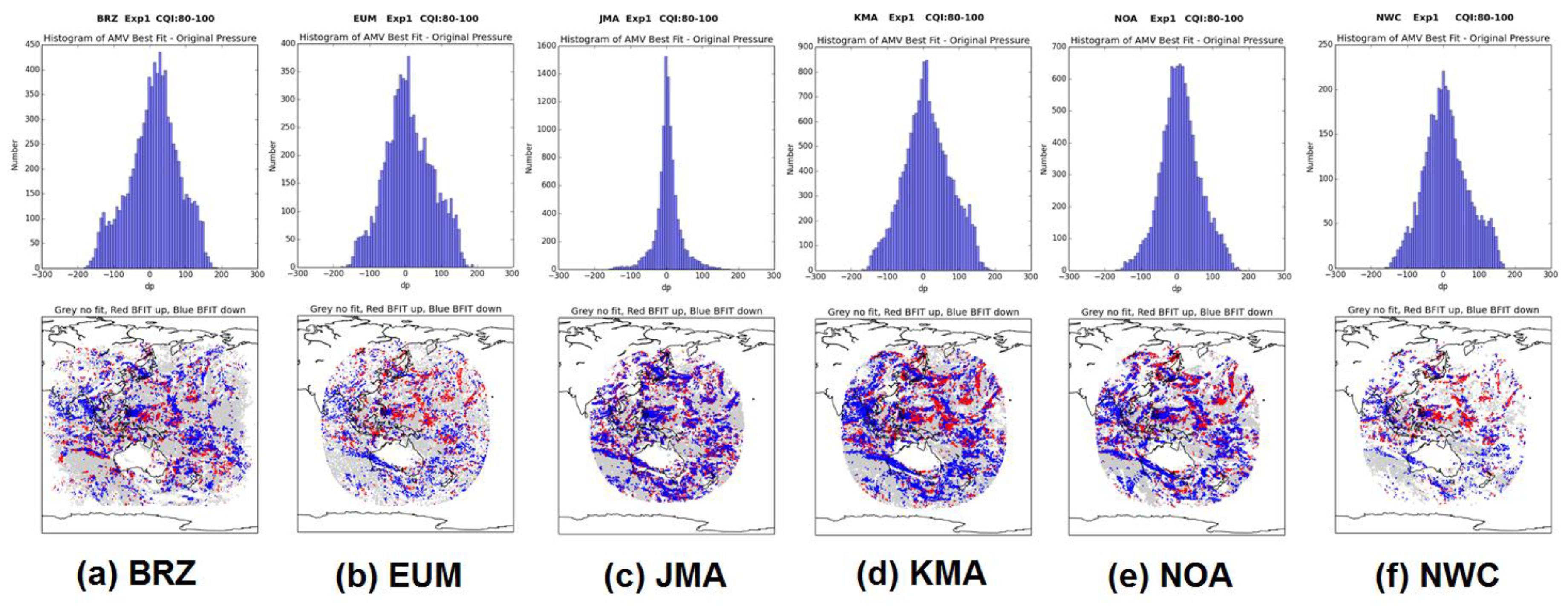
Figure 5.
Histogram (upper) and maps (lower) of the difference ‘AMV best-fit pressure level—AMV pressure level’ for (a) BRZ, (b) EUM, (c) JMA, (d) KMA, (e) NOA, (f) NWC. In the maps, red shows the best-fit pressure at a higher level; blue shows the best-fit pressure at a lower level.
Figure 5.
Histogram (upper) and maps (lower) of the difference ‘AMV best-fit pressure level—AMV pressure level’ for (a) BRZ, (b) EUM, (c) JMA, (d) KMA, (e) NOA, (f) NWC. In the maps, red shows the best-fit pressure at a higher level; blue shows the best-fit pressure at a lower level.
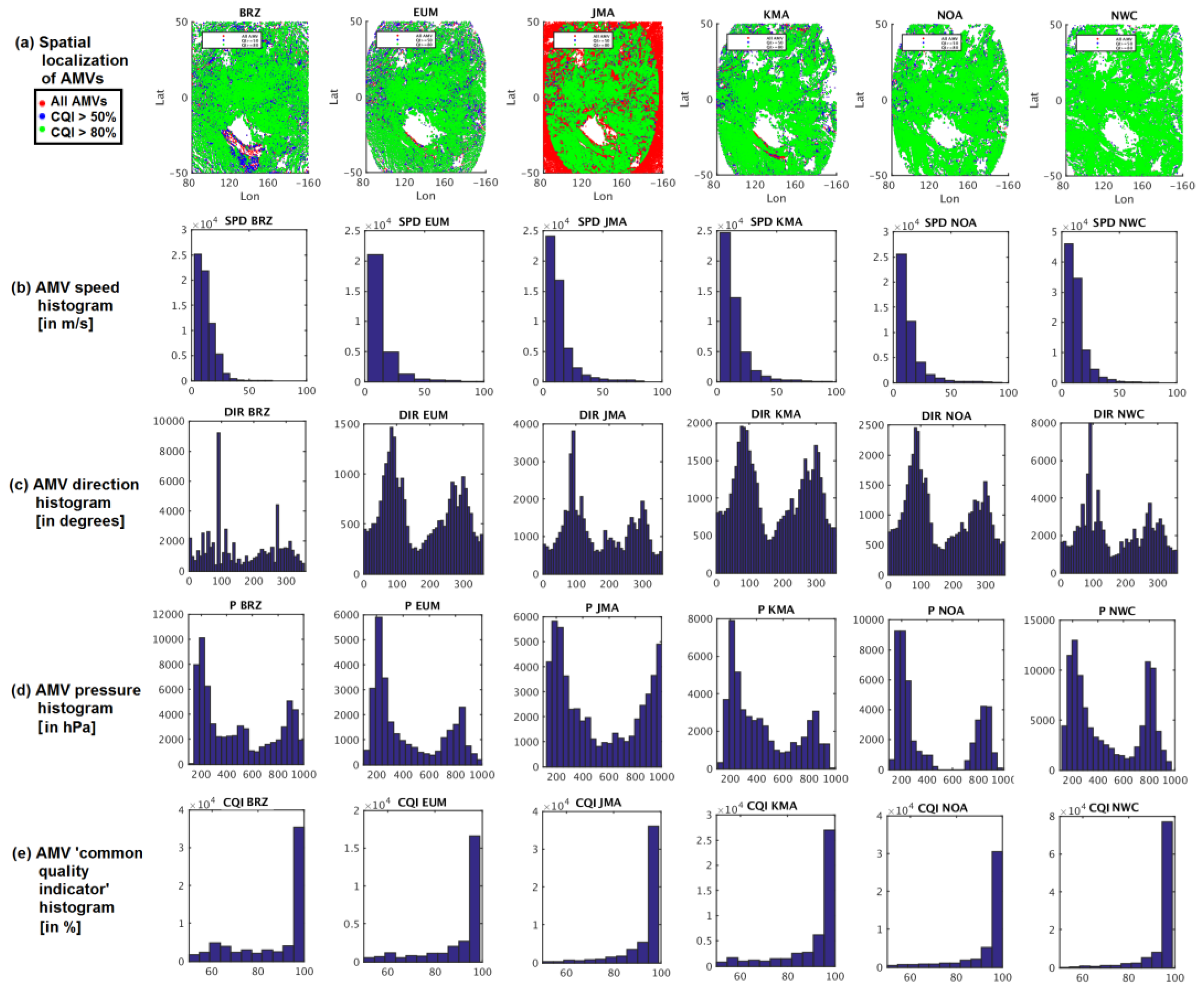
Figure 6.
Spatial localization of AMVs (a), and histograms of parameters: (b) AMV speed in m s−1, (c) AMV direction in degrees, (d) AMV pressure in hPa, (e) AMV CQI in %, for the AMV datasets in Experiment 2 with CQI >= 50%. From left to right, BRZ, EUM, JMA, KMA, NOA, NWC.
Figure 6.
Spatial localization of AMVs (a), and histograms of parameters: (b) AMV speed in m s−1, (c) AMV direction in degrees, (d) AMV pressure in hPa, (e) AMV CQI in %, for the AMV datasets in Experiment 2 with CQI >= 50%. From left to right, BRZ, EUM, JMA, KMA, NOA, NWC.
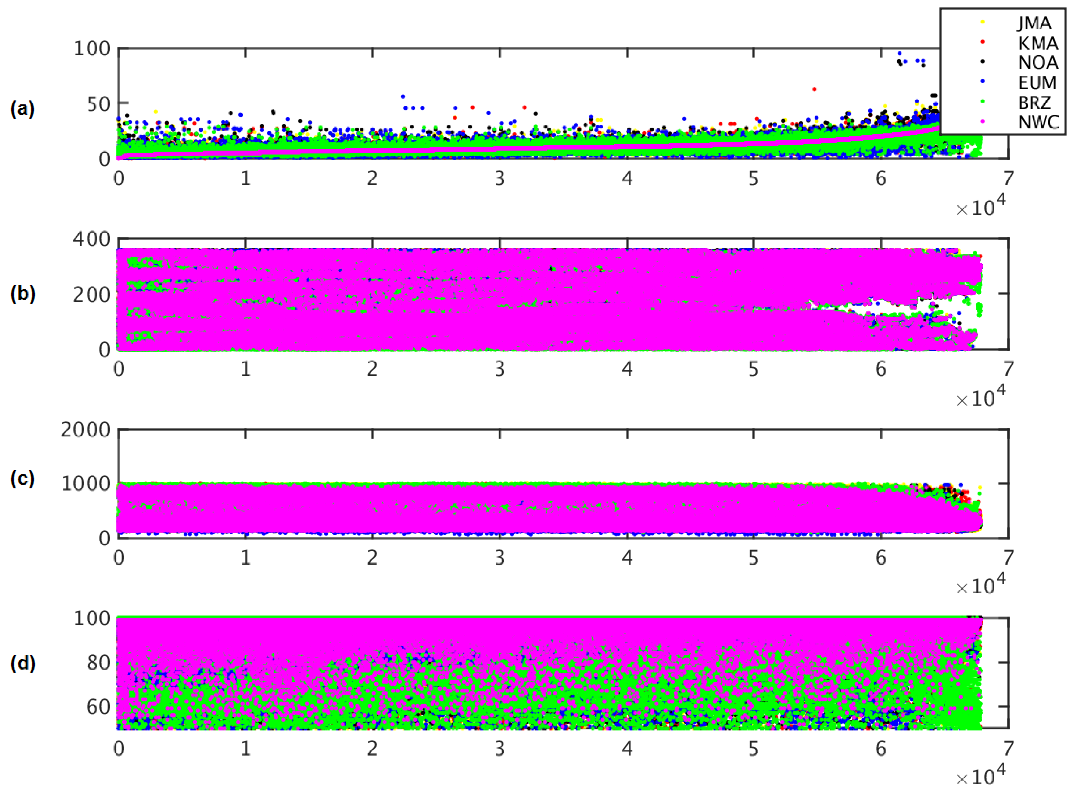
Figure 7.
‘Parameter plot’ for collocated AMVs from the different AMV datasets in Experiment 2, with CQI >= 50% and a collocation distance up to 55 km. Considered variables are speed (a), direction (b), pressure (c), and CQI (d). Color codes correspond to BRZ in green, EUM in blue, JMA in yellow, KMA in red, NOA in black, NWC in magenta.
Figure 8.
Scatterplot of collocated AMV pressures for Experiment 2, with CQI >= 50% and a collocation distance up to 55 km, for each center versus EUM AMV pressures (BRZ in green; JMA in yellow; KMA in red; NOA in black; NWC in magenta).
Figure 8.
Scatterplot of collocated AMV pressures for Experiment 2, with CQI >= 50% and a collocation distance up to 55 km, for each center versus EUM AMV pressures (BRZ in green; JMA in yellow; KMA in red; NOA in black; NWC in magenta).
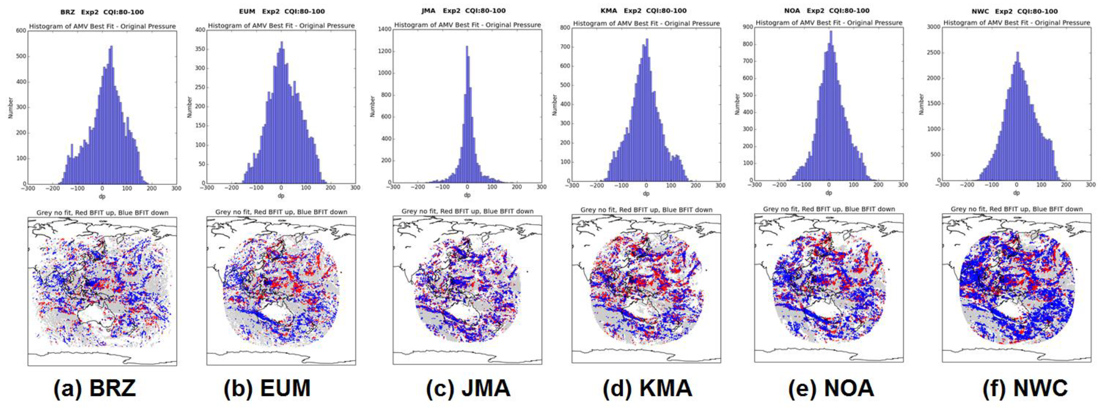
Figure 9.
Histogram (upper) and maps (lower) of the difference ‘AMV best-fit pressure level—AMV pressure level’ for (a) BRZ, (b) EUM, (c) JMA, (d) KMA, (e) NOA, (f) NWC. In the maps, red shows the best-fit pressure at a higher level; blue shows the best-fit pressure at a lower level.
Figure 9.
Histogram (upper) and maps (lower) of the difference ‘AMV best-fit pressure level—AMV pressure level’ for (a) BRZ, (b) EUM, (c) JMA, (d) KMA, (e) NOA, (f) NWC. In the maps, red shows the best-fit pressure at a higher level; blue shows the best-fit pressure at a lower level.
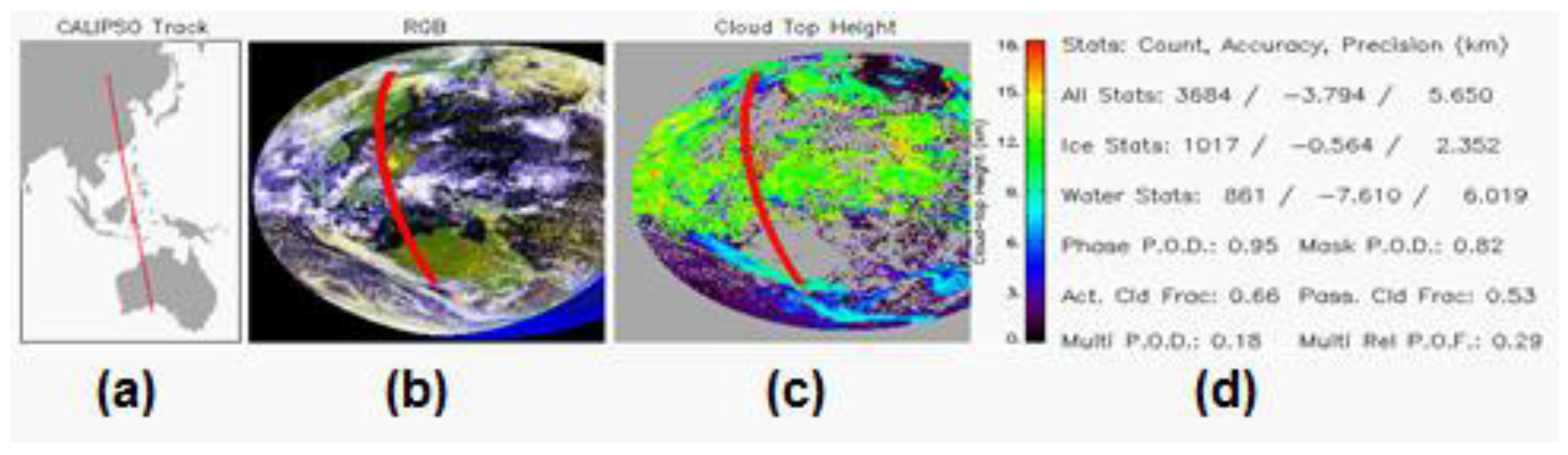
Figure 10.
CALIPSO (Cloud-Aerosol Lidar and Infrared Pathfinder Satellite Observation) data for 21 July 2016 at 0530-0550 UTC, used in Experiment 3: (a) Ground track over a map of the West Pacific Ocean, (b) Ground track over the corresponding Himawari-8 RGB image, (c) Ground track over the corresponding Himawari-8 derived Cloud top height, (d) Statistics for the CALIPSO data.
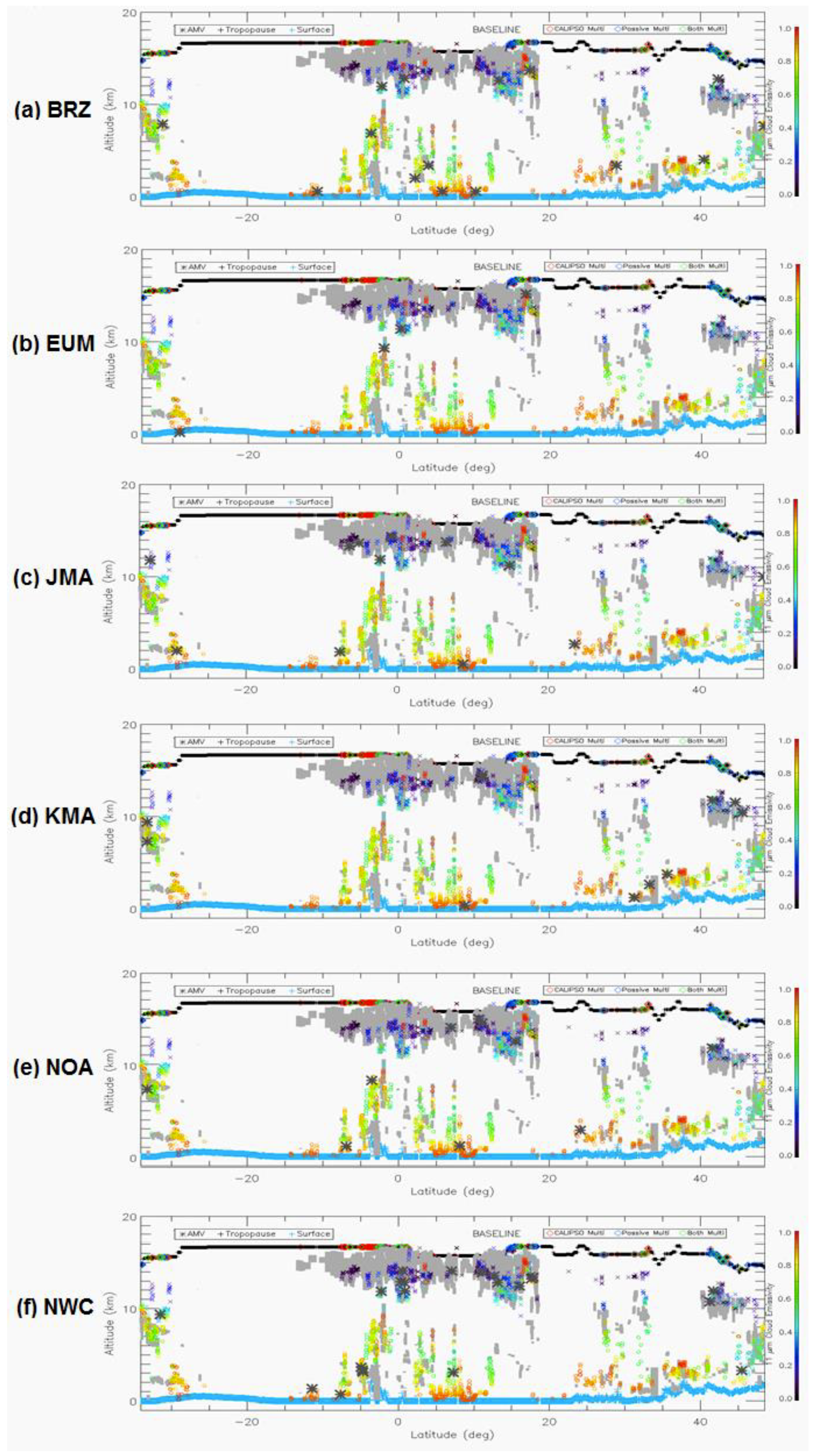
Figure 11.
Experiment 3: Collocation of AMVs (defined as black asterisks *) with CALIPSO cloud measurements for (a) BRZ, (b) EUM, (c) JMA, (d) KMA, (e) NOA, (f) NWC.
Figure 11.
Experiment 3: Collocation of AMVs (defined as black asterisks *) with CALIPSO cloud measurements for (a) BRZ, (b) EUM, (c) JMA, (d) KMA, (e) NOA, (f) NWC.
Table 1.
Reported variables for the AMVs (Atmospheric Motion Vectors) in all datasets.
Table 1.
Reported variables for the AMVs (Atmospheric Motion Vectors) in all datasets.
| Parameter | Code | Description |
|---|
| 1 | IDN | AMV Identification Number |
| 2 | LAT[degrees] | AMV Latitude |
| 3 | LON[degrees] | AMV Longitude |
| 4 | TS[pixels] | Target Box Size |
| 5 | SS[pixels] | Search Box Size |
| 6 | SPD[m/s] | AMV Speed |
| 7 | DIR[degrees] | AMV Direction
(0: due North, 90: due East, 180: due South, 270: due West) |
| 8 | PRES[hPa] | AMV Pressure |
| 9 | L | Low-Level Correction Flag
(0: No correction, 1: Inversion correction, 2: Cloud base) |
| 10 | NWPSPD[m/s] | Numerical Weather Prediction (NWP) Wind Speed Guess |
| 11 | NWPDIR[degrees] | Numerical Weather Prediction (NWP) Wind Direction Guess |
| 12 | ALB[%] | 0.8 μm Albedo at the Center Pixel of the Target Box |
| 13 | CORR[%] | Maximum Value of the Tracking Cross-correlation |
| 14 | T | Tracking Method Flag
(0: Cross-correlation, 1: Sum of squared differences, 2: Other) |
| 15 | PRESERR[hPa] | AMV Pressure Error |
| 16 | H | Height Assignment Method, as defined in page 4 of the text
(0: EBBT, 1: CO2 Slicing, 2: IR/WV ratioing, 3: CCC, 4: Other) |
| 17 | QINF[%] | Quality Indicator without Forecast |
| 18 | QIF[%] | Quality Indicator with Forecast |
| 19 | CQI[%] | Common Quality Indicator |
Table 2.
Parameter distribution for the different AMV datasets in Experiment 1 with CQI >= 50%.
Table 2.
Parameter distribution for the different AMV datasets in Experiment 1 with CQI >= 50%.
| | BRZ | EUM | JMA | KMA | NOA | NWC |
|---|
| Total Number of AMVs | 70,312 | 30,868 | 76,075 | 58,479 | 38,242 | 14,602 |
| Common Quality Index >= 50% | 57,613 | 27,097 | 33,717 | 52,685 | 36,172 | 14,283 |
| Speed min. (m/s) | 2.56 | 2.51 | 2.50 | 2.50 | 3.00 | 2.50 |
| Speed max. (m/s) | 66.05 | 139.93 | 69.97 | 97.01 | 92.29 | 68.77 |
| Speed mean (m/s) | 11.81 | 13.64 | 13.29 | 13.66 | 14.06 | 13.64 |
| Pressure min. (hPa) | 100.00 | 57.11 | 125.00 | 102.08 | 102.05 | 101.00 |
| Pressure max. (hPa) | 1000.00 | 1004.00 | 994.32 | 997.66 | 977.82 | 965.50 |
| Pressure mean (hPa) | 533.19 | 437.37 | 496.89 | 408.80 | 432.19 | 386.40 |
| Percentage of Low AMVs (%) | 37.10 | 26.66 | 31.43 | 23.05 | 33.77 | 23.61 |
| Percentage of Mid AMVs (%) | 20.33 | 14.56 | 19.34 | 13.29 | 2.63 | 8.96 |
| Percentage of High AMVs (%) | 42.57 | 58.78 | 49.23 | 63.66 | 63.59 | 67.43 |
| Speed min. of Low AMVs (m/s) | 2.56 | 2.52 | 2.50 | 2.50 | 3.00 | 2.57 |
| Speed max. of Low AMVs (m/s) | 35.67 | 99.02 | 41.20 | 70.19 | 40.52 | 28.57 |
| Speed mean of Low AMVs (m/s) | 9.61 | 9.33 | 9.06 | 9.67 | 10.21 | 9.95 |
| Pressure min. of Low AMVs (hPa) | 700.00 | 700.23 | 700.01 | 700.00 | 700.06 | 700.00 |
| Pressure max. of Low AMVs (hPa) | 1000.00 | 1004.00 | 994.32 | 997.66 | 977.82 | 965.50 |
| Pressure mean of Low AMVs (hPa) | 874.49 | 823.71 | 888.89 | 820.21 | 837.59 | 782.70 |
| Speed min. of Mid AMVs (m/s) | 2.61 | 2.53 | 2.50 | 2.50 | 3.06 | 2.51 |
| Speed max. of Mid AMVs (m/s) | 66.05 | 94.60 | 69.25 | 70.08 | 78.86 | 48.12 |
| Speed mean of Mid AMVs (m/s) | 13.61 | 14.58 | 14.03 | 14.53 | 22.14 | 17.05 |
| Pressure min. of Mid AMVs (hPa) | 400.02 | 400.03 | 400.01 | 400.03 | 400.01 | 400.05 |
| Pressure max. of Mid AMVs (hPa) | 699.98 | 699.77 | 699.99 | 699.90 | 449.96 | 699.50 |
| Pressure mean of Mid AMVs (hPa) | 536.33 | 531.56 | 528.20 | 521.45 | 425.91 | 536.54 |
| Speed min. of High AMVs (m/s) | 2.58 | 2.51 | 2.50 | 2.50 | 3.00 | 2.50 |
| Speed max. of High AMVs (m/s) | 62.47 | 139.93 | 69.97 | 97.01 | 92.29 | 68.77 |
| Speed mean of High AMVs (m/s) | 12.88 | 15.37 | 15.69 | 14.92 | 15.77 | 14.47 |
| Pressure min. of High AMVs (hPa) | 100.00 | 57.11 | 125.00 | 102.08 | 102.05 | 101.00 |
| Pressure max. of High AMVs (hPa) | 400.00 | 399.94 | 399.98 | 399.97 | 399.99 | 400.00 |
| Pressure mean of High AMVs (hPa) | 234.17 | 238.80 | 234.32 | 236.29 | 217.14 | 227.70 |
Table 3.
Experiment 1: Comparison of AMVs, with CQI >= 50%, to radiosonde winds within 150 km. (N = Number of Matches; Pre Bias = Pressure Bias; Pre RMS = Pressure Root Mean Square Error; Spd Bias = Wind Speed Bias; Spd RMS = Wind Speed Root Mean Square Error; Dir Bias = Wind Direction Bias; Vec RMS = Wind Vector Root Mean Square Error). The extremes for each category are highlighted; in yellow, the worst value, and in green, the best value.
| | N | Pre Bias | Pre RMS | Spd Bias | Spd RMS | Dir Bias | Vec RMS |
|---|
| BRZ | 774 | 0.90 | 14.68 | −1.28 | 10.00 | −13.13 | 12.61 |
| EUM | 443 | −1.63 | 16.52 | −1.74 | 7.86 | 8.69 | 12.67 |
| JMA | 400 | 0.50 | 13.81 | −0.91 | 3.95 | 1.30 | 5.74 |
| KMA | 859 | −0.55 | 15.16 | −1.88 | 7.61 | 5.46 | 10.10 |
| NOA | 512 | −1.05 | 14.15 | −0.86 | 6.29 | 1.10 | 8.16 |
| NWC | 163 | −0.69 | 15.11 | −1.14 | 4.99 | −1.47 | 6.80 |
Table 4.
The same as
Table 3, but with CQI >= 80%.
Table 4.
The same as
Table 3, but with CQI >= 80%.
| | N | Pre Bias | Pre RMS | Spd Bias | Spd RMS | Dir Bias | Vec RMS |
|---|
| BRZ | 448 | 0.02 | 13.97 | 0.31 | 6.07 | −14.61 | 8.62 |
| EUM | 312 | −0.83 | 16.54 | −1.79 | 6.54 | 8.31 | 8.56 |
| JMA | 344 | 0.78 | 13.77 | −1.07 | 4.07 | 1.09 | 5.93 |
| KMA | 666 | −0.79 | 15.51 | −1.56 | 6.42 | 2.78 | 8.97 |
| NOA | 427 | −1.49 | 13.96 | −0.89 | 5.42 | 0.45 | 7.52 |
| NWC | 132 | −0.41 | 15.08 | −0.97 | 5.01 | −5.98 | 6.94 |
Table 5.
Experiment 1: Comparison of collocated AMVs with QINF >= 80%, with NWP analysis winds. (N = Number of AMVs; NBF = Number of AMVs with Best-Fit Pressure Value; VD = Vector Difference for all AMVs; VDBF = Vector Difference for AMVs with Best-Fit Pressure Value; RMS = Root Mean Square Error for all AMVs; RMSBF = Root Mean Square Error for AMVs with Best-Fit Pressure Value). The extremes for each category are highlighted; in yellow, the worst value, and in green, the best value.
| | N | NBF | VD | VDBF | RMS | RMSBF |
|---|
| BRZ | 4930 | 1191 | 5.90 | 5.27 | 8.47 | 8.16 |
| EUM | 4930 | 1625 | 3.96 | 3.19 | 4.93 | 4.28 |
| JMA | 4930 | 1793 | 2.48 | 2.24 | 2.96 | 2.77 |
| KMA | 4930 | 1732 | 3.69 | 2.85 | 4.61 | 3.79 |
| NOA | 4930 | 1757 | 3.45 | 2.76 | 4.30 | 3.73 |
| NWC | 4930 | 1763 | 3.95 | 3.09 | 4.70 | 3.95 |
Table 6.
Experiment 1: The same as
Table 5, but with Common Quality Indicator >= 80%.
Table 6.
Experiment 1: The same as
Table 5, but with Common Quality Indicator >= 80%.
| | N | NBF | VD | VDBF | RMS | RMSBF |
|---|
| BRZ | 8076 | 2122 | 5.54 | 4.85 | 7.53 | 7.13 |
| EUM | 8076 | 2655 | 4.04 | 3.24 | 4.97 | 4.28 |
| JMA | 8076 | 2860 | 2.59 | 2.33 | 3.10 | 2.89 |
| KMA | 8076 | 2802 | 3.80 | 2.97 | 4.73 | 3.94 |
| NOA | 8076 | 2854 | 3.54 | 2.82 | 4.36 | 3.74 |
| NWC | 8076 | 2791 | 3.99 | 3.17 | 4.74 | 4.03 |
Table 7.
Experiment 1: Comparison of all AMVs to NWP analysis winds, with a CQI threshold so that at least 10,000 AMVs are kept. (CQI = Common Quality Indicator Threshold used for each center; N = Number of AMVs; NBF = Number of AMVs with Best-Fit Pressure Value; VD = Vector Difference for all AMVs; VDBF = Vector Difference for AMVs with Best-Fit Pressure Value; RMS = Root Mean Square Error for all AMVs; RMSBF = Root Mean Square Error for AMVs with Best-Fit Pressure Value). The extremes for each category are highlighted; in yellow, the worst value, and in green, the best value.
| | CQI | N | NBF | VD | VDBF | RMS | RMSBF |
|---|
| BRZ | 100 | 18355 | 3946 | 4.71 | 4.14 | 6.62 | 6.21 |
| EUM | 98 | 11120 | 3712 | 4.80 | 3.83 | 6.90 | 6.19 |
| JMA | 99 | 11805 | 4353 | 2.52 | 2.27 | 3.19 | 3.02 |
| KMA | 99 | 19170 | 7166 | 4.74 | 3.63 | 6.57 | 5.65 |
| NOA | 99 | 14086 | 5342 | 3.78 | 2.89 | 5.07 | 4.27 |
| NWC | 90 | 10117 | 3669 | 4.25 | 3.28 | 5.21 | 4.31 |
Table 8.
Experiment 1: Speed Bias (BIAS) and Speed Standard Deviation (STD) with respect to the NWP analysis winds, before and after the best-fit pressure level correction, for all AMVs for which the best-fit pressure level correction could be applied, with QINF >= 80%. The extremes for each category are highlighted; in yellow, the worst value, and in green, the best value.
| | BIAS before | STD before | BIAS after | STD after |
|---|
| BRZ | −1.00 | 4.38 | 0.28 | 1.16 |
| EUM | −0.15 | 4.65 | 0.26 | 1.19 |
| JMA | 0.06 | 1.79 | 0.21 | 1.11 |
| KMA | −0.12 | 4.42 | 0.21 | 1.14 |
| NOA | −0.04 | 3.77 | 0.23 | 1.17 |
| NWC | 0.13 | 3.97 | 0.27 | 1.18 |
Table 9.
The same as
Table 8, but with CQI >= 80%.
Table 9.
The same as
Table 8, but with CQI >= 80%.
| | BIAS before | STD before | BIAS after | STD after |
|---|
| BRZ | −1.12 | 4.33 | 0.25 | 1.16 |
| EUM | −0.20 | 4.57 | 0.26 | 1.18 |
| JMA | 0.05 | 1.78 | 0.22 | 1.11 |
| KMA | −0.33 | 4.55 | 0.21 | 1.14 |
| NOA | −0.04 | 3.77 | 0.23 | 1.17 |
| NWC | −0.25 | 4.01 | 0.23 | 1.16 |
Table 10.
Parameter distribution for the different AMV datasets in experiment 2 with CQI >= 50%.
Table 10.
Parameter distribution for the different AMV datasets in experiment 2 with CQI >= 50%.
| | BRZ | EUM | JMA | KMA | NOA | NWC |
|---|
| Total Number of AMVs | 74,100 | 30,806 | 67,324 | 53,171 | 47,320 | 146,780 |
| Common Quality Index >= 50% | 65,673 | 28,174 | 27,057 | 47,411 | 45,782 | 146,496 |
| Speed min. (m/s) | 2.55 | 2.50 | 2.51 | 2.50 | 3.00 | 2.50 |
| Speed max. (m/s) | 70.06 | 145.55 | 85.94 | 97.01 | 94.16 | 84.03 |
| Speed mean (m/s) | 12.02 | 13.37 | 14.00 | 13.89 | 13.97 | 12.97 |
| Pressure min. (hPa) | 100.00 | 57.58 | 125.02 | 106.81 | 105.72 | 101.00 |
| Pressure max. (hPa) | 1000.00 | 1009.80 | 996.47 | 1000.00 | 987.20 | 972.50 |
| Pressure mean (hPa) | 487.06 | 438.03 | 497.74 | 450.50 | 432.01 | 409.12 |
| Percentage of Low AMVs (%) | 29.96 | 27.15 | 32.27 | 24.56 | 33.55 | 25.63 |
| Percentage of Mid AMVs (%) | 21.19 | 14.14 | 17.51 | 22.02 | 2.56 | 11.52 |
| Percentage of High AMVs (%) | 48.85 | 58.71 | 50.22 | 53.42 | 63.89 | 62.86 |
| Speed min. of Low AMVs (m/s) | 2.55 | 2.50 | 2.51 | 2.50 | 3.01 | 2.50 |
| Speed max. of Low AMVs (m/s) | 46.46 | 54.21 | 32.67 | 70.27 | 37.59 | 36.22 |
| Speed mean of Low AMVs (m/s) | 9.39 | 8.89 | 9.14 | 10.54 | 9.77 | 8.76 |
| Pressure min. of Low AMVs (hPa) | 700.00 | 700.06 | 700.04 | 700.00 | 700.08 | 700.00 |
| Pressure max. of Low AMVs (hPa) | 1000.00 | 1009.80 | 996.47 | 1000.00 | 987.20 | 972.50 |
| Pressure mean of Low AMVs (hPa) | 870.56 | 820.69 | 887.37 | 817.99 | 835.02 | 788.38 |
| Speed min. of Mid AMVs (m/s) | 2.55 | 2.51 | 2.51 | 2.50 | 3.04 | 2.51 |
| Speed max. of Mid AMVs (m/s) | 69.46 | 69.67 | 72.05 | 80.01 | 69.25 | 62.00 |
| Speed mean of Mid AMVs (m/s) | 13.73 | 13.95 | 14.46 | 15.11 | 21.30 | 14.95 |
| Pressure min. of Mid AMVs (hPa) | 400.03 | 400.06 | 400.00 | 400.02 | 400.06 | 400.50 |
| Pressure max. of Mid AMVs (hPa) | 699.97 | 699.73 | 699.97 | 699.98 | 449.98 | 699.50 |
| Pressure mean of Mid AMVs (hPa) | 528.14 | 529.96 | 533.05 | 514.73 | 426.70 | 535.47 |
| Speed min. of High AMVs (m/s) | 2.59 | 2.50 | 2.52 | 2.50 | 3.00 | 2.50 |
| Speed max. of High AMVs (m/s) | 70.06 | 145.55 | 85.94 | 97.01 | 94.16 | 84.03 |
| Speed mean of High AMVs (m/s) | 12.88 | 15.31 | 16.97 | 14.92 | 15.88 | 14.33 |
| Pressure min. of High AMVs (hPa) | 100.00 | 57.58 | 125.02 | 106.81 | 105.72 | 101.00 |
| Pressure max. of High AMVs (hPa) | 400.00 | 399.94 | 399.98 | 400.00 | 399.97 | 400.00 |
| Pressure mean of High AMVs (hPa) | 233.99 | 238.96 | 235.09 | 255.08 | 220.57 | 231.35 |
Table 11.
Experiment 2: Comparison of AMVs, with CQI >= 50%, to radiosonde winds within 150 km. (N = Number of Matches; Pre Bias = Pressure Bias; Pre RMS = Pressure Root Mean Square Error; Spd Bias = Wind Speed Bias; Spd RMS = Wind Speed Root Mean Square Error; Dir Bias = Wind Direction Bias; Vec RMS = Wind Vector Root Mean Square Error). The extremes for each category are highlighted; in yellow, the worst value, and in green, the best value.
| | N | Pre Bias | Pre RMS | Spd Bias | Spd RMS | Dir Bias | Vec RMS |
|---|
| BRZ | 942 | 1.46 | 14.44 | −2.69 | 11.65 | −9.48 | 15.22 |
| EUM | 508 | −0.62 | 15.92 | −2.17 | 7.03 | 10.08 | 8.87 |
| JMA | 313 | −2.94 | 18.33 | −1.36 | 4.64 | −0.83 | 6.34 |
| KMA | 797 | −0.64 | 14.80 | −1.55 | 7.78 | −1.41 | 10.03 |
| NOA | 691 | −1.58 | 13.93 | −0.90 | 5.44 | 1.89 | 7.62 |
| NWC | 2204 | −1.02 | 16.30 | −2.17 | 6.03 | 0.40 | 7.85 |
Table 12.
The same as
Table 11, but with Common Quality indicator (CQI) >= 80%.
Table 12.
The same as
Table 11, but with Common Quality indicator (CQI) >= 80%.
| | N | Pre Bias | Pre RMS | Spd Bias | Spd RMS | Dir Bias | Vec RMS |
|---|
| BRZ | 619 | 1.16 | 13.44 | −0.40 | 7.36 | −14.65 | 9.80 |
| EUM | 366 | −0.66 | 14.74 | −2.20 | 6.15 | 8.43 | 8.56 |
| JMA | 270 | −3.43 | 18.67 | −1.40 | 4.64 | −0.83 | 5.93 |
| KMA | 628 | −0.84 | 14.30 | −1.21 | 7.39 | −2.66 | 8.97 |
| NOA | 599 | −1.69 | 13.98 | −0.88 | 5.25 | 0.39 | 7.52 |
| NWC | 2063 | −1.19 | 16.19 | −2.11 | 5.99 | 0.79 | 6.94 |
Table 13.
Experiment 2: Comparison of collocated AMVs, with QINF >= 80%, to NWP analysis winds. (N = Number of AMVs; NBF = Number of AMVs with Best-Fit Pressure Value; VD = Vector Difference for all AMVs; VDBF = Vector Difference for AMVs with Best-Fit Pressure Value; RMS = Root Mean Square Error for all AMVs; RMSBF = Root Mean Square Error for AMVs with Best-Fit Pressure Value. The extremes for each category are highlighted; in yellow, the worst value, and in green, the best value.
| | N | NBF | VD | VDBF | RMS | RMSBF |
|---|
| BRZ | 43281 | 9814 | 5.60 | 5.01 | 8.20 | 7.90 |
| EUM | 43281 | 13270 | 3.84 | 3.05 | 4.96 | 4.24 |
| JMA | 43281 | 14572 | 2.20 | 1.99 | 2.71 | 2.52 |
| KMA | 43281 | 12709 | 3.75 | 3.08 | 5.05 | 4.51 |
| NOA | 43281 | 13765 | 3.41 | 2.74 | 4.26 | 3.64 |
| NWC | 43281 | 13588 | 3.45 | 2.79 | 4.13 | 3.54 |
Table 14.
Experiment 2: The same as
Table 13, but with CQI >= 80%.
Table 14.
Experiment 2: The same as
Table 13, but with CQI >= 80%.
| | N | NBF | VD | VDBF | RMS | RMSBF |
|---|
| BRZ | 56515 | 13075 | 5.73 | 5.11 | 8.35 | 8.02 |
| EUM | 56515 | 17533 | 4.00 | 3.17 | 5.17 | 4.43 |
| JMA | 56515 | 19208 | 2.27 | 2.06 | 2.80 | 2.62 |
| KMA | 56515 | 16635 | 3.92 | 3.23 | 5.25 | 4.72 |
| NOA | 56515 | 18163 | 3.53 | 2.84 | 4.42 | 3.80 |
| NWC | 56515 | 17860 | 3.55 | 2.87 | 4.24 | 3.65 |
Table 15.
Experiment 2: Comparison of all AMVs to NWP analysis winds, with a CQI threshold so that at least 10,000 AMVs are kept. (CQI = Common Quality Indicator Threshold used for each center; N = Number of AMVs; NBF = Number of AMVs with Best-Fit Pressure Value; VD = Vector Difference for all AMVs; VDBF = Vector Difference for AMVs with Best-Fit Pressure Value; RMS = Root Mean Square Error for all AMVs; RMSBF = Root Mean Square Error for AMVs with Best-Fit Pressure Value). The extremes for each category are highlighted; in yellow, the worst value, and in green, the best value.
| | CQI | N | NBF | VD | VDBF | RMS | RMSBF |
|---|
| BRZ | 100 | 26341 | 5733 | 5.90 | 5.22 | 8.32 | 7.91 |
| EUM | 98 | 12407 | 4056 | 4.43 | 3.46 | 6.13 | 5.28 |
| JMA | 98 | 10595 | 3991 | 2.52 | 2.29 | 3.20 | 3.03 |
| KMA | 99 | 16721 | 5934 | 4.66 | 3.75 | 6.71 | 6.06 |
| NOA | 100 | 14484 | 5484 | 3.84 | 2.91 | 5.06 | 4.21 |
| NWC | 99 | 80625 | 28532 | 4.24 | 3.26 | 5.24 | 4.36 |
Table 16.
Experiment 2: Speed Bias (BIAS) and Speed Standard Deviation (STD) with respect to the NWP analysis winds, before and after the best-fit pressure level correction, for all AMVs for which the best-fit pressure level correction could be applied with QINF >= 80%. The extremes for each category are highlighted; in yellow, the worst value, and in green, the best value.
| | BIAS before | STD before | BIAS after | STD after |
|---|
| BRZ | −1.51 | 4.57 | 0.26 | 1.17 |
| EUM | −0.28 | 4.60 | 0.18 | 1.17 |
| JMA | 0.09 | 1.82 | 0.20 | 1.14 |
| KMA | 0.65 | 3.89 | 0.23 | 1.14 |
| NOA | −0.22 | 3.82 | 0.24 | 1.15 |
| NWC | −0.32 | 3.94 | 0.20 | 1.14 |
Table 17.
The same as
Table 16, but with CQI >= 80%.
Table 17.
The same as
Table 16, but with CQI >= 80%.
| | BIAS before | STD before | BIAS after | STD after |
|---|
| BRZ | −1.57 | 4.56 | 0.26 | 1.16 |
| EUM | −0.20 | 4.57 | 0.26 | 1.18 |
| JMA | 0.07 | 1.82 | 0.21 | 1.12 |
| KMA | 0.60 | 3.97 | 0.22 | 1.15 |
| NOA | −0.22 | 3.82 | 0.24 | 1.15 |
| NWC | −0.68 | 4.10 | 0.18 | 1.12 |
Table 18.
Similarities found in the AMV datasets by the ‘paired t-test’ for the different combinations of variables and AMV datasets, in Experiment 1 (with prescribed configuration).
Table 18.
Similarities found in the AMV datasets by the ‘paired t-test’ for the different combinations of variables and AMV datasets, in Experiment 1 (with prescribed configuration).
| Prescribed Configuration | Speed | Direction | Pressure | Quality Indicator | ALL |
|---|
| QINF >= 50% | 4 | 6 | 1 | 0 | 11 |
| QINF >= 80% | 6 | 5 | 1 | 1 | 13 |
| CQI >= 50% | 1 | 3 | 0 | 1 | 5 |
| CQI >= 80% | 2 | 6 | 1 | 1 | 10 |
Table 19.
Similarities found in the AMV datasets by the ‘paired t-test’ for the different combinations of variables and AMV datasets, in Experiment 2 (with specific configuration).
Table 19.
Similarities found in the AMV datasets by the ‘paired t-test’ for the different combinations of variables and AMV datasets, in Experiment 2 (with specific configuration).
| Specific Configuration | Speed | Direction | Pressure | Quality Indicator | ALL |
|---|
| QINF >= 50% | 1 | 2 | 0 | 0 | 3 |
| QINF >= 80% | 1 | 2 | 2 | 0 | 5 |
| CQI >= 50% | 1 | 2 | 0 | 0 | 3 |
| CQI >= 80% | 1 | 1 | 0 | 1 | 3 |

 ,
, 


