AdTree: Accurate, Detailed, and Automatic Modelling of Laser-Scanned Trees


Abstract
1. Introduction
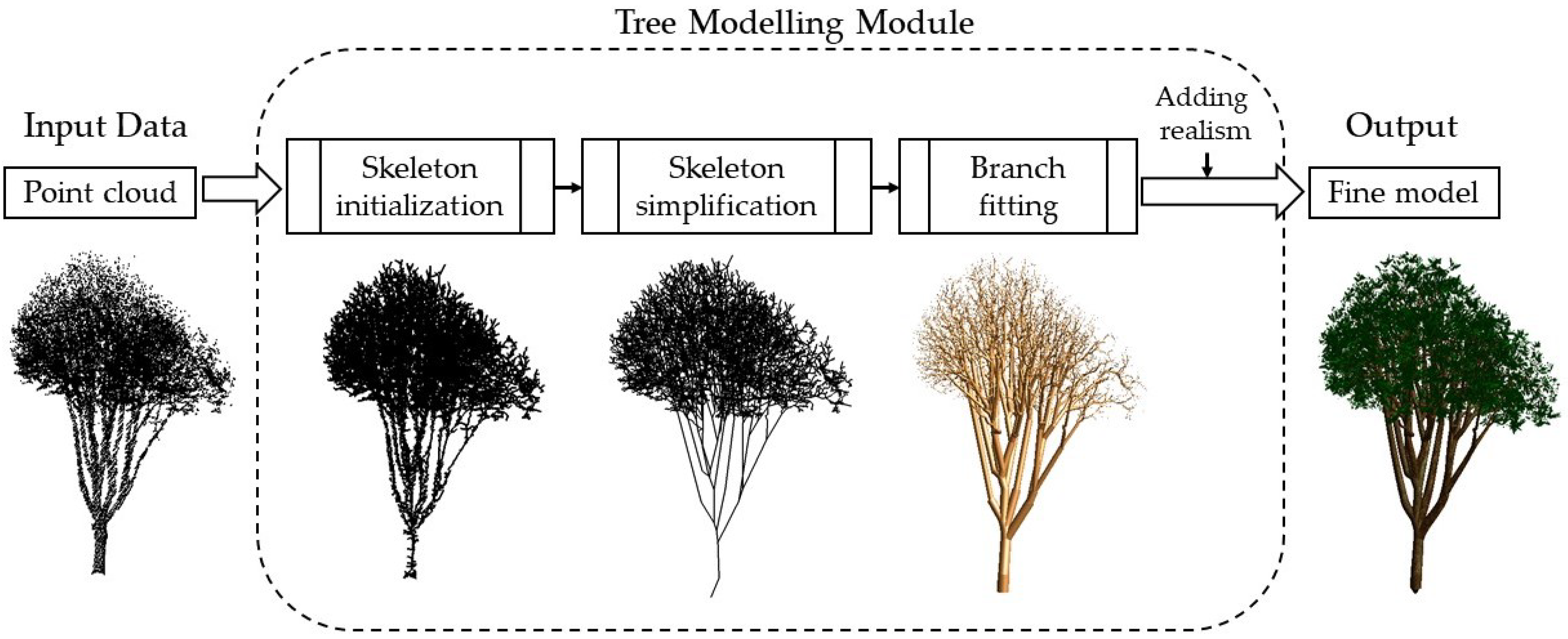
2. Overview
- Robust to tree species. The method should be able to reconstruct common tree species with clear branch structures. The reconstructed models should convey the main topological branch structure of the real world trees represented by the point clouds. Vegetation that do not demonstrate skeleton structures (e.g., bushes) are not considered the target objects.
- High fidelity. The reconstructed tree models should be topologically faithful to the input and have acceptable geometrical accuracy. This is vital for applications where important tree attributes (i.e., stem location, stem thickness, tree height) are expected to be derived from the reconstructed models.
- High efficiency. The reconstruction process should not require user intervention, i.e., it is fully automatic and can produce 3D models of individual trees promptly regardless of the size of the input point clouds. This enables large scale tree modeling when, for instance, an instance segmentation of the trees is available [24].
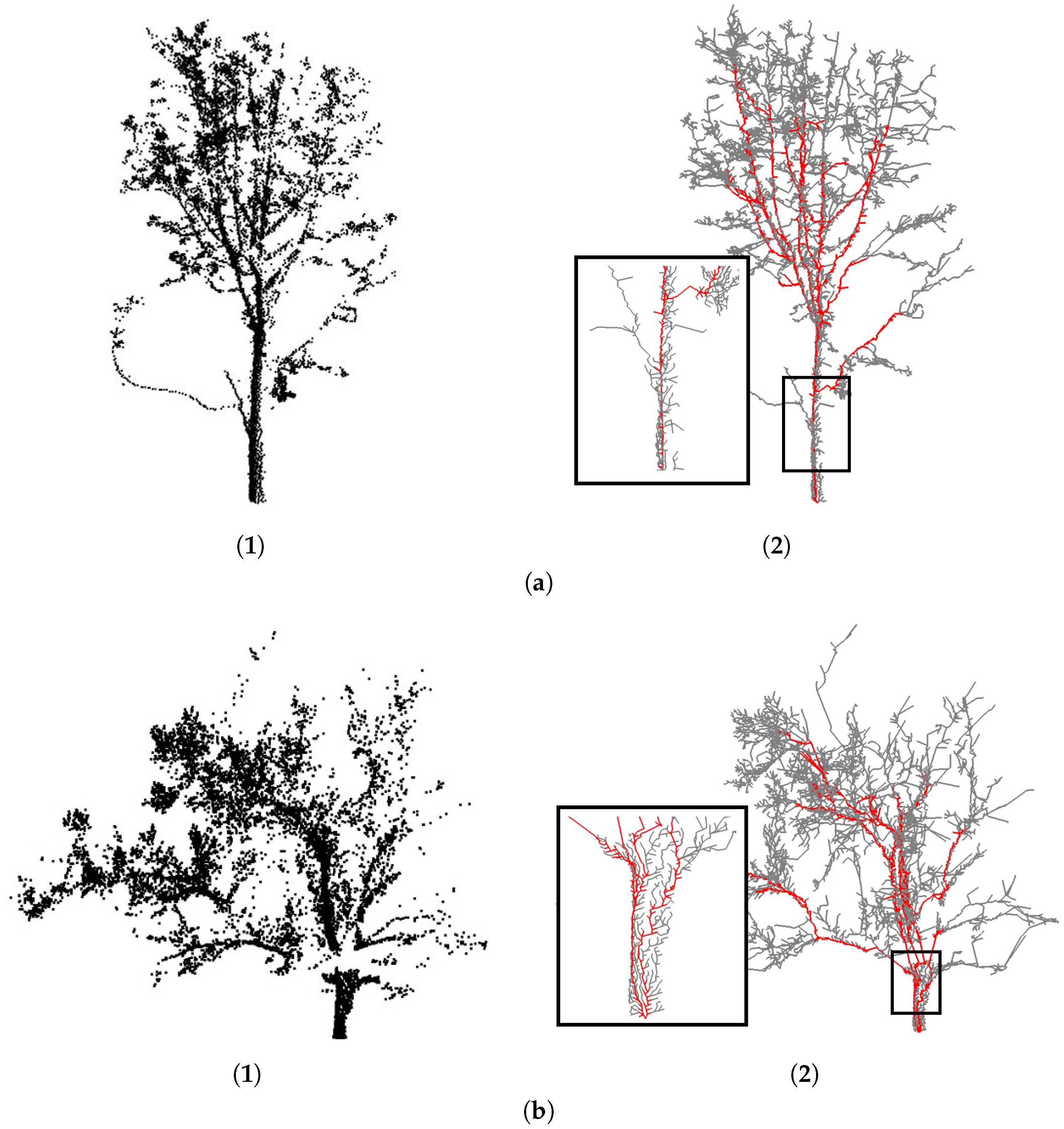
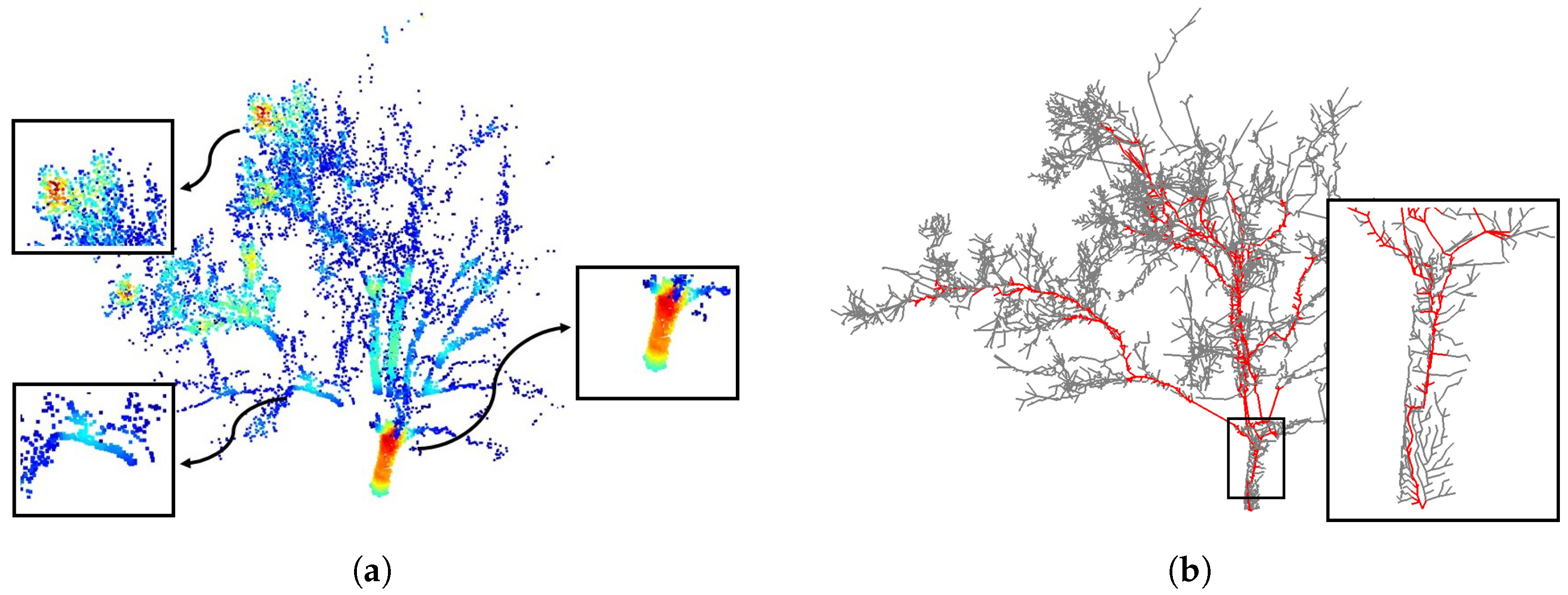
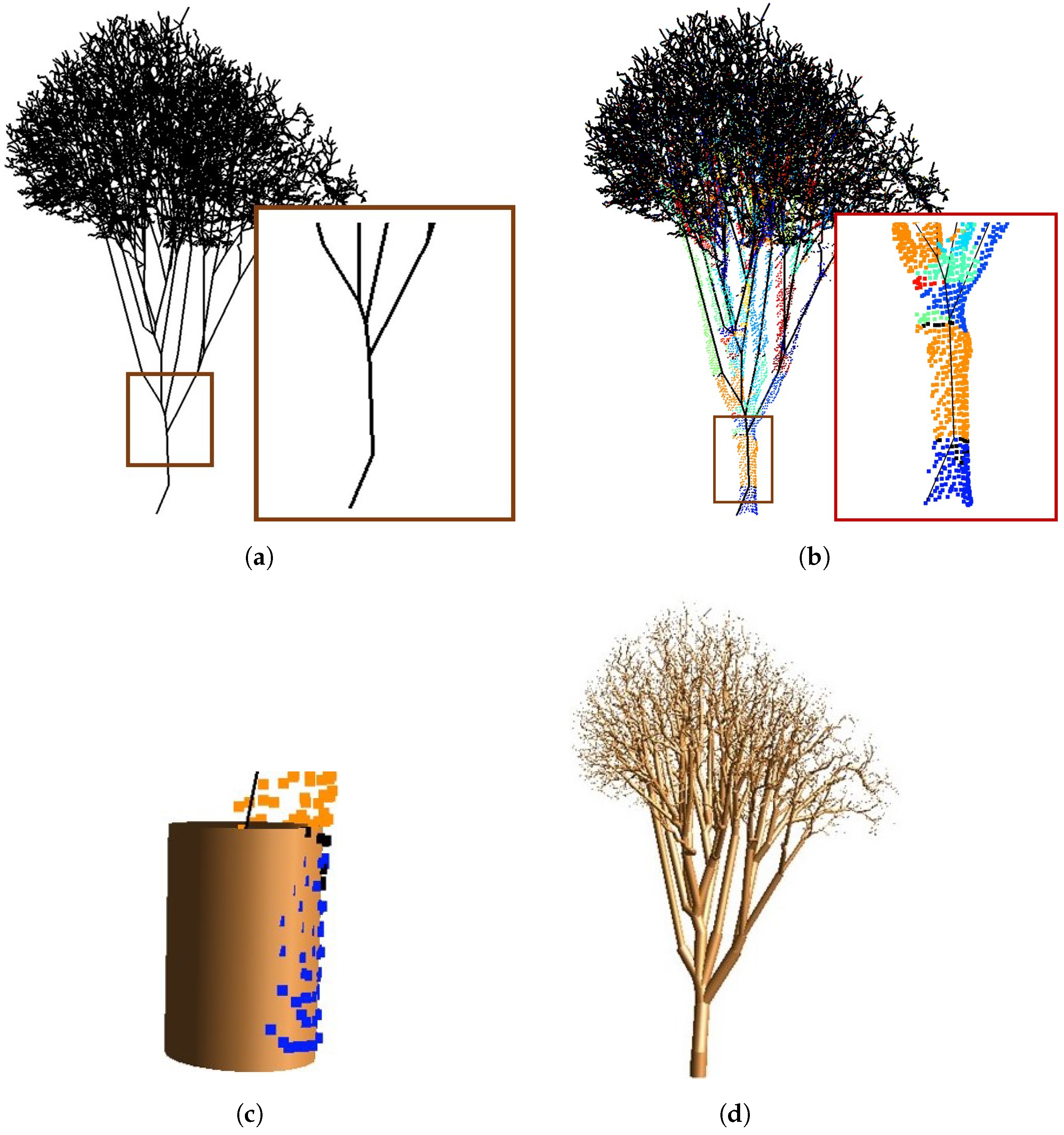
- Skeleton initialization. We triangulate the input points and apply the MST algorithm to extract the initial tree skeleton. Note that the main-branch points are identified and centralized beforehand to improve the quality of the skeleton;
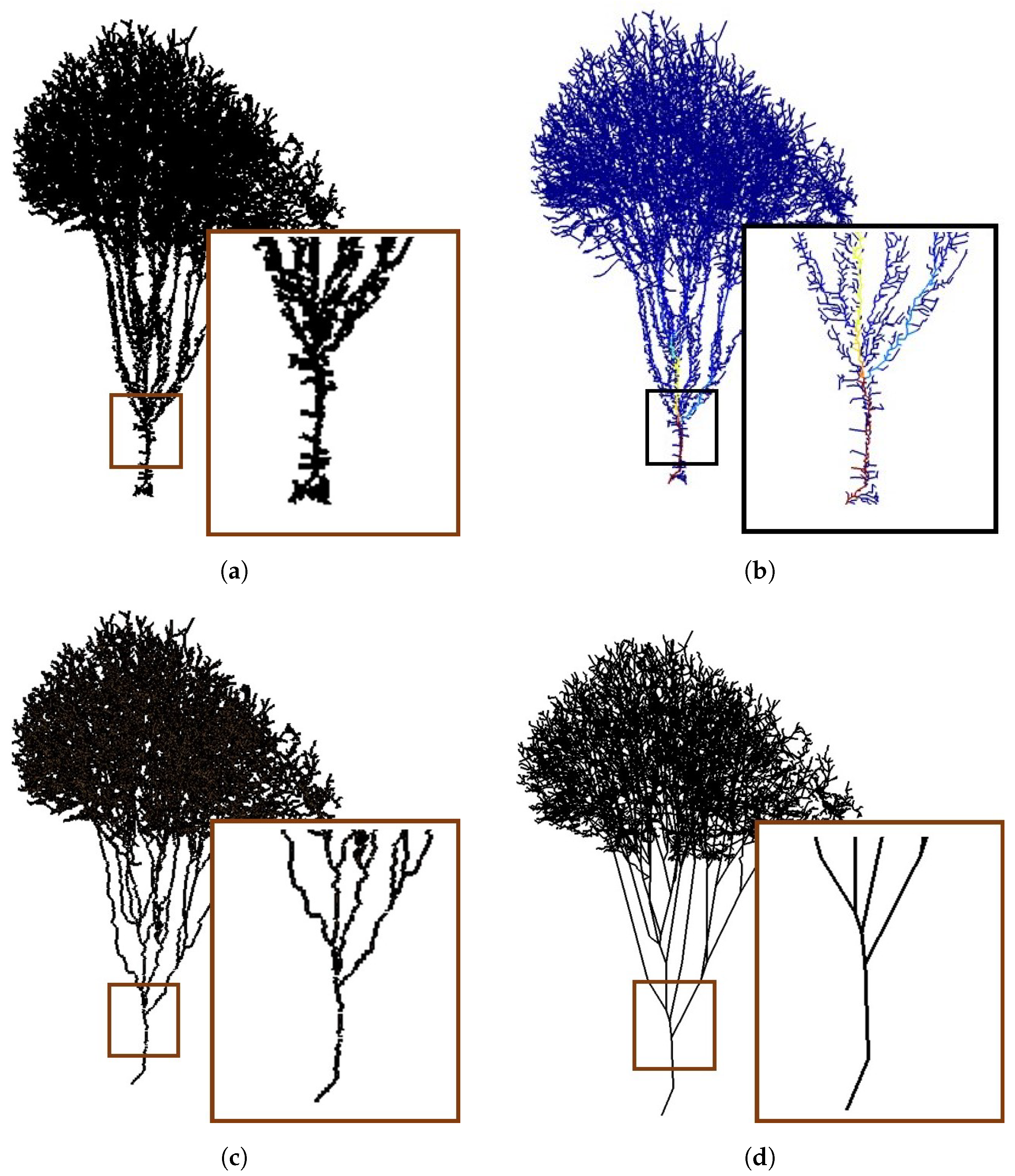
- Skeleton simplification. The initial skeleton is iteratively simplified, resulting in a light-weight tree skeleton. We simplify the skeleton by retrieving and merging adjacent vertices if their distance is sufficiently small;
- Branch fitting. Based on the reconstructed tree skeleton, we fit a sequence of cylinders over the input points to approximate the geometry of the branches. We first apply non-linear least squares to obtain the accurate radius of the tree trunk. Then, we derive the radius of the subsequent branches from the main trunk geometry;
- Adding realism. We synthesize leaves at the end of tree branches and add texture to enhance realism.
3. Materials and Methods
3.1. Skeleton Initialization
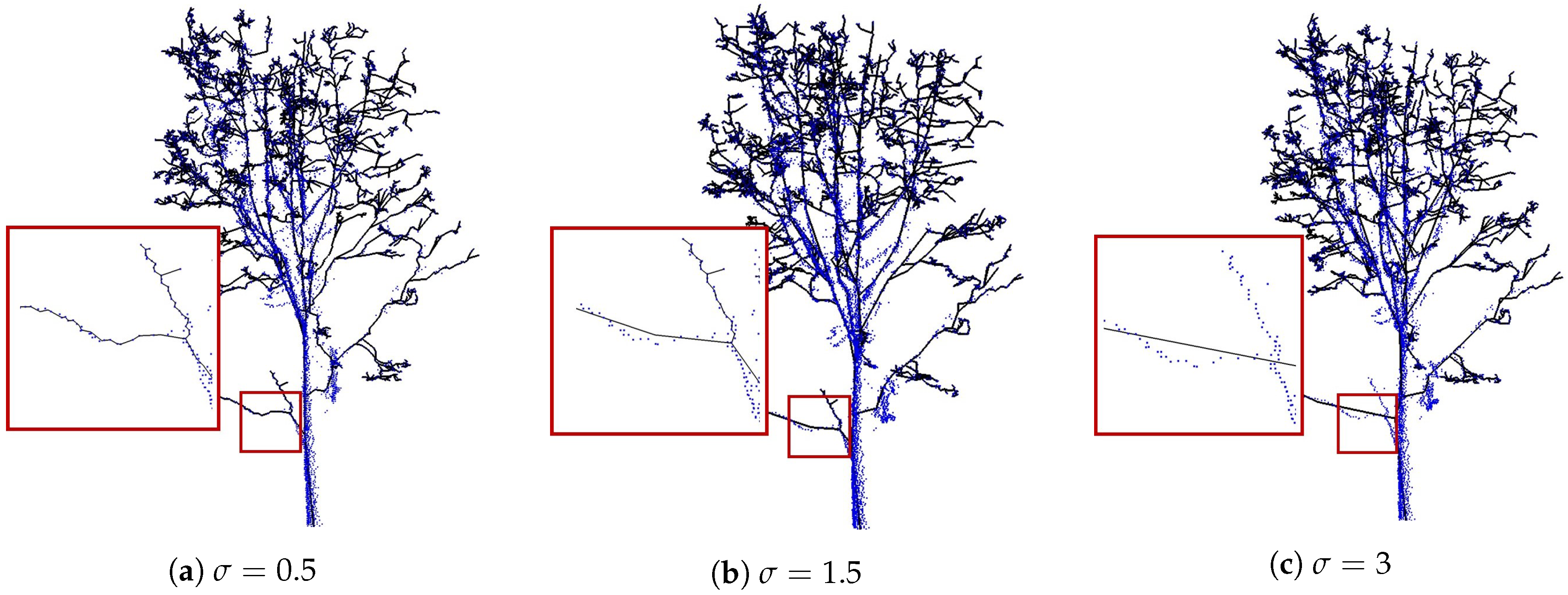
3.2. Skeleton Simplification
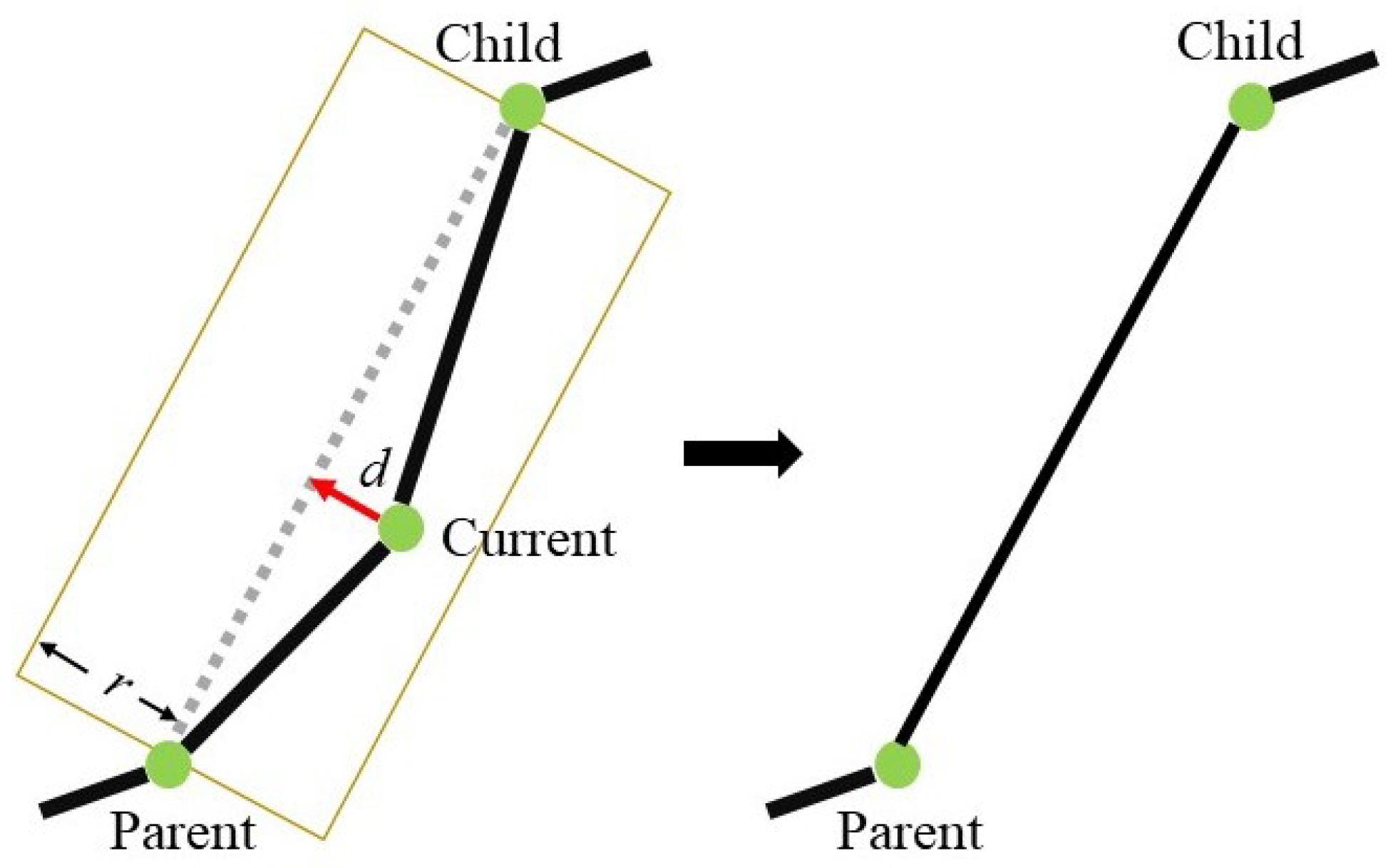
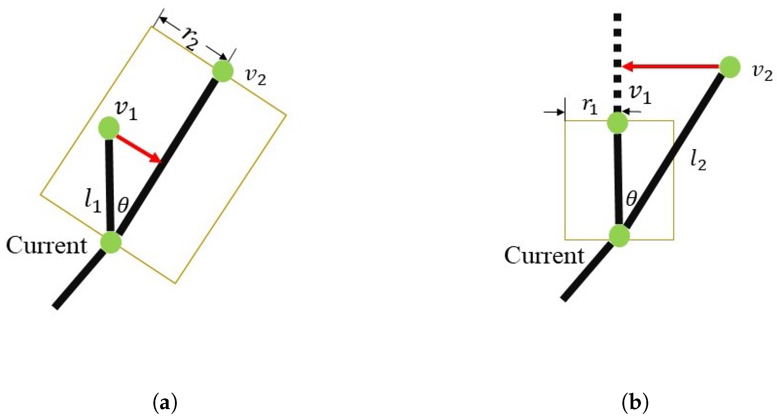
3.2.1. Assigning Vertex and Edge Importances
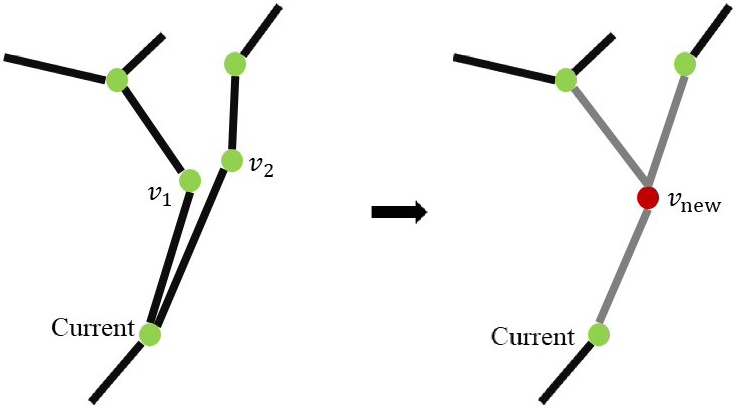
3.2.2. Simplifying Adjacent Vertices and Edges
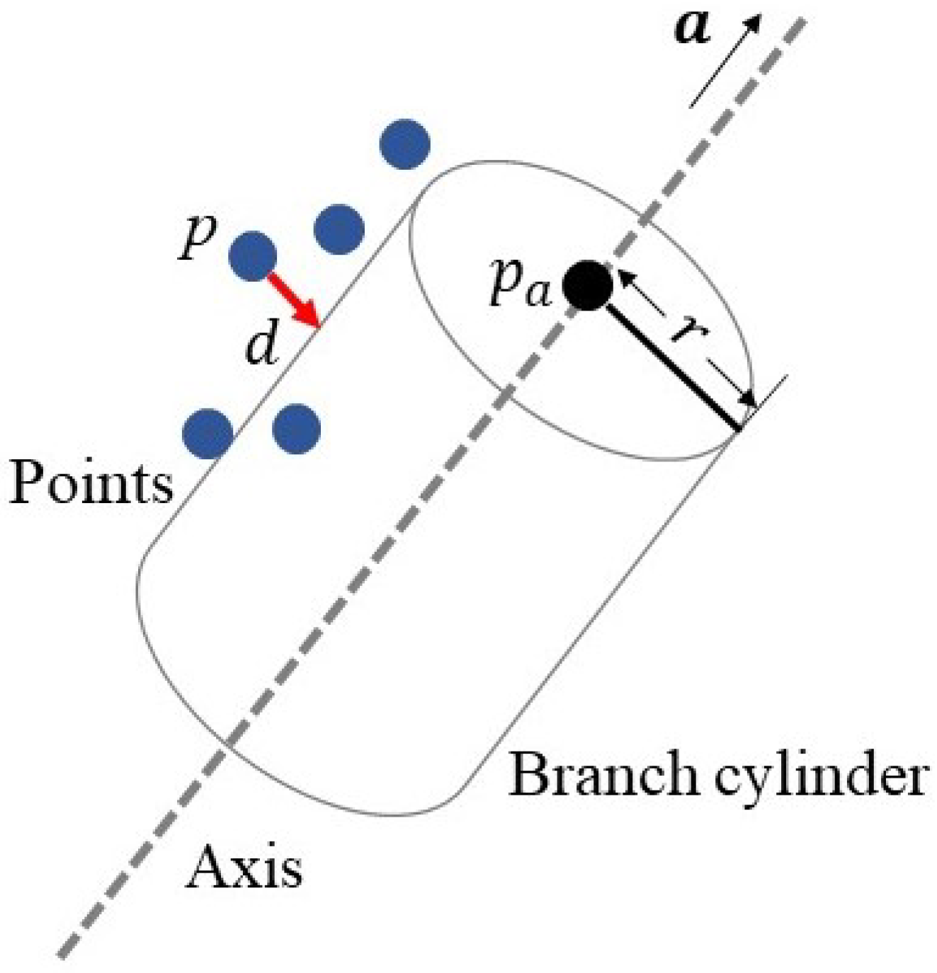
3.3. Branch Fitting
- Input data: position p of the input points;
- Parameters to be solved: the axis direction vector of the cylinder, position of the endpoint on the axis, and the radius r of the cylinder;
- Objective function: sum of squared distance d from the points to the branch cylinder, i.e.,
3.4. Adding Realism
3.5. Implementation Details
3.6. Test Datasets
4. Results and Discussion
4.1. Visual Evaluation
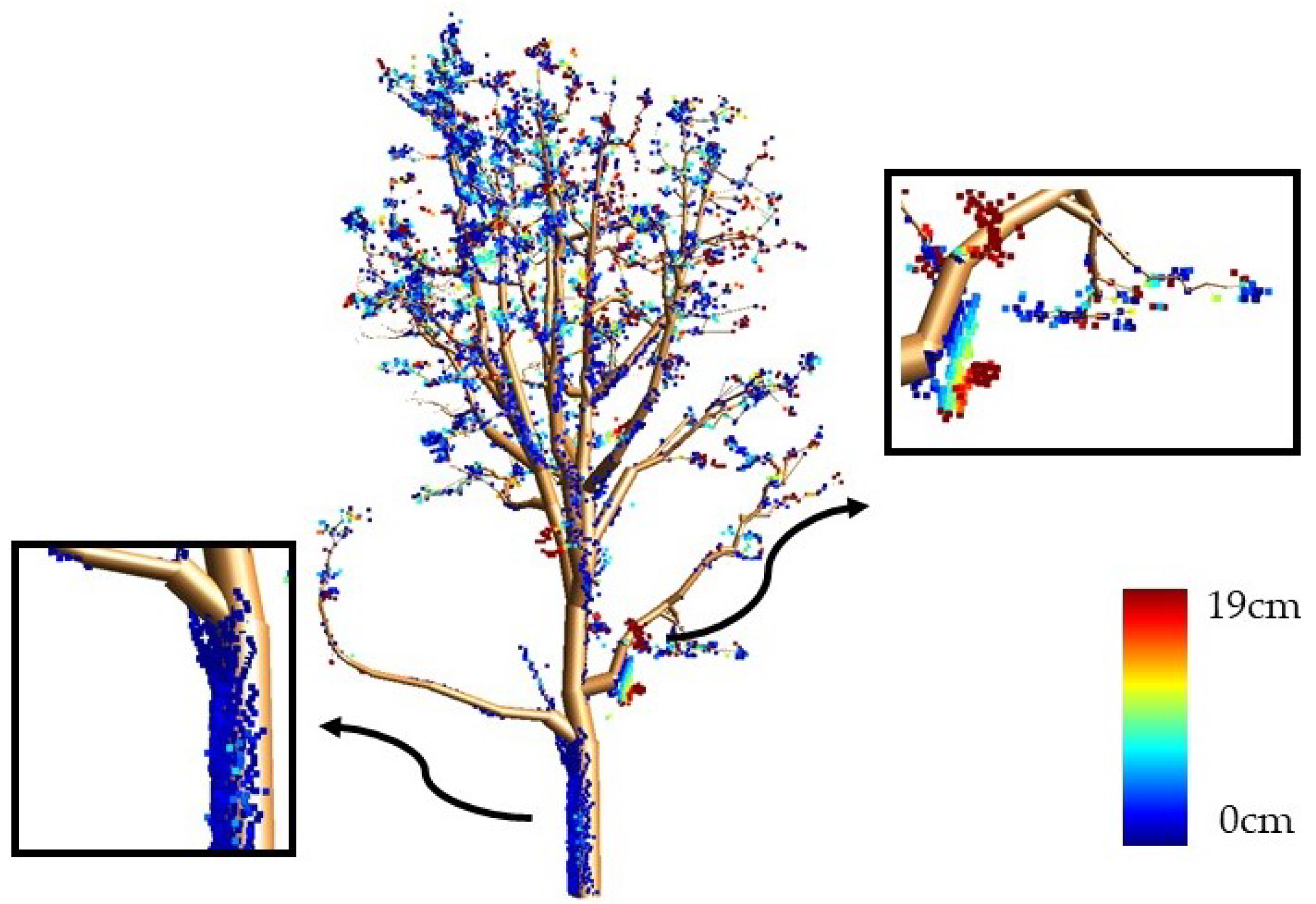
4.2. Reconstruction Accuracy
4.3. Robustness
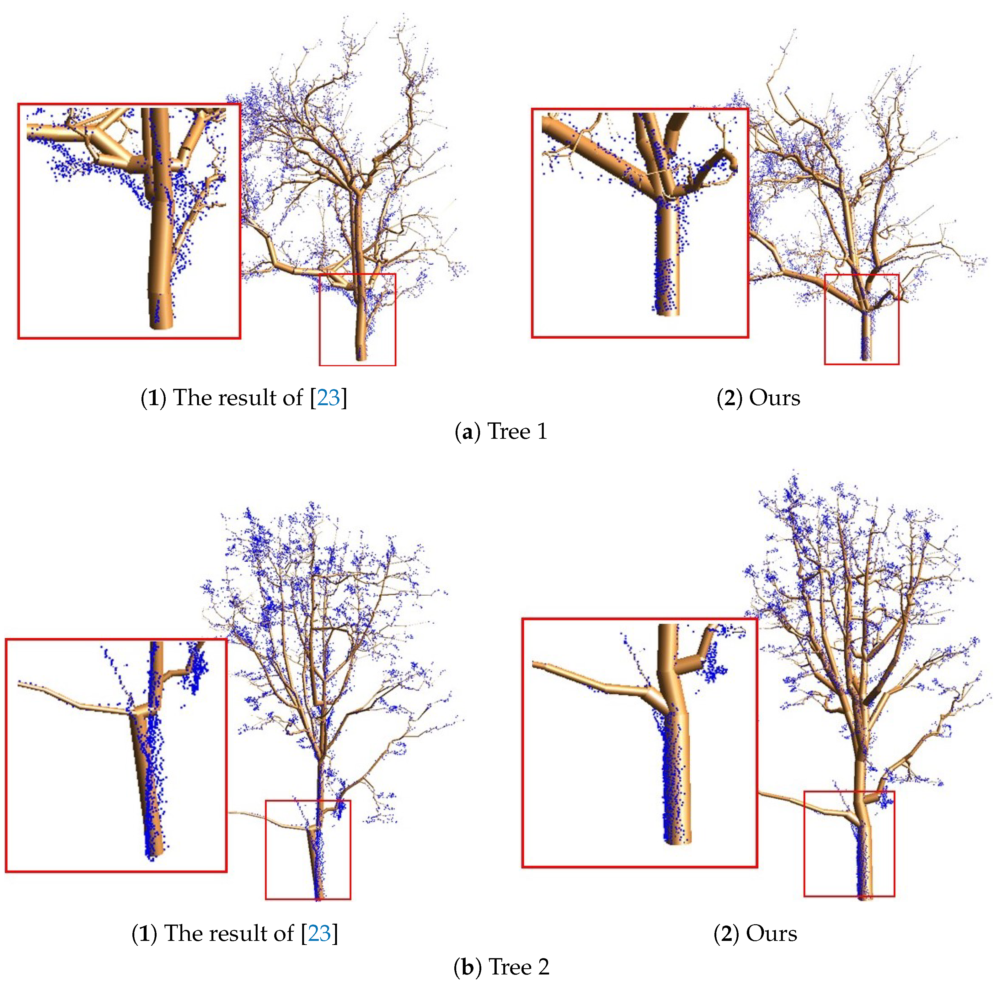
4.4. Comparisons
4.5. Limitations
4.6. Potential Applications
5. Conclusions and Future Work
Author Contributions
Funding
Acknowledgments
Conflicts of Interest
Abbreviations
| LiDAR | Light Detection and Ranging |
| MST | Minimum Spanning Tree |
| PCA | Principal Component Analysis |
| QSM | Quantitative Structure Modelling |
| SFM | Structure From Motion |
References
- Deussen, O.; Hanrahan, P.; Lintermann, B.; Měch, R.; Pharr, M.; Prusinkiewicz, P. Realistic modeling and rendering of plant ecosystems. In Proceedings of the 25th Annual Conference on Computer Graphics and Interactive Techniques, Orlando, FL, USA, 19–24 July 1998; pp. 275–286. [Google Scholar]
- Maltamo, M.; Næsset, E.; Vauhkonen, J. Forestry applications of airborne laser scanning. Concept Case Stud. Manag. For Ecosys 2014, 27, 460. [Google Scholar]
- Ke, Y.; Quackenbush, L.J. A review of methods for automatic individual tree-crown detection and delineation from passive remote sensing. Int. J. Remote Sens. 2011, 32, 4725–4747. [Google Scholar] [CrossRef]
- Hyyppa, J.; Kelle, O.; Lehikoinen, M.; Inkinen, M. A segmentation-based method to retrieve stem volume estimates from 3-D tree height models produced by laser scanners. IEEE Trans. Geosci. Remote Sens. 2001, 39, 969–975. [Google Scholar] [CrossRef]
- Kamal, M.; Phinn, S.; Johansen, K. Object-based approach for multi-scale mangrove composition mapping using multi-resolution image datasets. Remote Sens. 2015, 7, 4753–4783. [Google Scholar] [CrossRef]
- Reche-Martinez, A.; Martin, I.; Drettakis, G. Volumetric reconstruction and interactive rendering of trees from photographs. ACM Trans. Gr. (ToG) 2004, 23, 720–727. [Google Scholar] [CrossRef]
- Shlyakhter, I.; Rozenoer, M.; Dorsey, J.; Teller, S. Reconstructing 3D tree models from instrumented photographs. IEEE Comput. Gr. Appl. 2001, 21, 53–61. [Google Scholar] [CrossRef]
- Quan, L.; Tan, P.; Zeng, G.; Yuan, L.; Wang, J.; Kang, S.B. Image-based plant modeling. ACM Trans. Gr. (TOG) 2006, 25, 599–604. [Google Scholar] [CrossRef]
- Guo, J.; Xu, S.; Yan, D.M.; Cheng, Z.; Jaeger, M.; Zhang, X. Realistic Procedural Plant Modeling from Multiple View Images. IEEE Trans. Vis. Comput. Gr. 2018. [Google Scholar] [CrossRef]
- Liang, X.; Kankare, V.; Hyyppä, J.; Wang, Y.; Kukko, A.; Haggrén, H.; Yu, X.; Kaartinen, H.; Jaakkola, A.; Guan, F.; et al. Terrestrial laser scanning in forest inventories. ISPRS J. Photogramm. Remote Sens. 2016, 115, 63–77. [Google Scholar] [CrossRef]
- Olofsson, K.; Holmgren, J.; Olsson, H. Tree stem and height measurements using terrestrial laser scanning and the RANSAC algorithm. Remote Sens. 2014, 6, 4323–4344. [Google Scholar] [CrossRef]
- Brandtberg, T.; Warner, T.A.; Landenberger, R.E.; McGraw, J.B. Detection and analysis of individual leaf-off tree crowns in small footprint, high sampling density lidar data from the eastern deciduous forest in North America. Remote Sens. Environ. 2003, 85, 290–303. [Google Scholar] [CrossRef]
- Holmgren, J.; Persson, Å. Identifying species of individual trees using airborne laser scanner. Remote Sens. Environ. 2004, 90, 415–423. [Google Scholar] [CrossRef]
- Wang, D.; Hollaus, M.; Puttonen, E.; Pfeifer, N. Automatic and self-adaptive stem reconstruction in landslide-affected forests. Remote Sens. 2016, 8, 974. [Google Scholar] [CrossRef]
- Hackenberg, J.; Spiecker, H.; Calders, K.; Disney, M.; Raumonen, P. SimpleTree—An efficient open source tool to build tree models from TLS clouds. Forests 2015, 6, 4245–4294. [Google Scholar] [CrossRef]
- Raumonen, P.; Kaasalainen, M.; Åkerblom, M.; Kaasalainen, S.; Kaartinen, H.; Vastaranta, M.; Holopainen, M.; Disney, M.; Lewis, P. Fast automatic precision tree models from terrestrial laser scanner data. Remote Sens. 2013, 5, 491–520. [Google Scholar] [CrossRef]
- Bucksch, A.; Lindenbergh, R.; Menenti, M. SkelTre. Vis. Comput. 2010, 26, 1283–1300. [Google Scholar] [CrossRef]
- Yan, D.M.; Wintz, J.; Mourrain, B.; Wang, W.; Boudon, F.; Godin, C. Efficient and robust reconstruction of botanical branching structure from laser scanned points. In Proceedings of the 2009 11th IEEE International Conference on Computer-Aided Design and Computer Graphics, Huangshan, China, 19–21 August 2009; pp. 572–575. [Google Scholar]
- Xu, H.; Gossett, N.; Chen, B. Knowledge and heuristic-based modeling of laser-scanned trees. ACM Trans. Gr. (TOG) 2007, 26, 19. [Google Scholar] [CrossRef]
- Verroust, A.; Lazarus, F. Extracting skeletal curves from 3D scattered data. In Proceedings of the Shape Modeling International’99, International Conference on Shape Modeling and Applications, Aizu-Wakamatsu, Japan, 1–4 March 1999; pp. 194–201. [Google Scholar]
- Delagrange, S.; Jauvin, C.; Rochon, P. PypeTree: A tool for reconstructing tree perennial tissues from point clouds. Sensors 2014, 14, 4271–4289. [Google Scholar] [CrossRef] [PubMed]
- Dey, T.K.; Sun, J. Defining and computing curve-skeletons with medial geodesic function. Symp. Geom. Process. 2006, 6, 143–152. [Google Scholar]
- Livny, Y.; Yan, F.; Olson, M.; Chen, B.; Zhang, H.; El-Sana, J. Automatic reconstruction of tree skeletal structures from point clouds. ACM Trans. Gr. (TOG) 2010, 29, 151. [Google Scholar]
- Xu, Y.; Sun, Z.; Hoegner, L.; Stilla, U.; Yao, W. Instance Segmentation of Trees in Urban Areas from MLS Point Clouds Using Supervoxel Contexts and Graph-Based Optimization. In Proceedings of the 2018 10th IAPR Workshop on Pattern Recognition in Remote Sensing, Beijing, China, 19–20 August 2018; pp. 1–5. [Google Scholar]
- Zhou, H.; Shenoy, N.; Nicholls, W. Efficient minimum spanning tree construction without Delaunay triangulation. In Proceedings of the 2001 Asia and South Pacific Design Automation Conference, Yokohama, Japan, 2 February 2001; pp. 192–197. [Google Scholar]
- Cheng, Y. Mean shift, mode seeking, and clustering. IEEE Trans. Pattern Anal. Mach. Intell. 1995, 17, 790–799. [Google Scholar] [CrossRef]
- Chi, Y.; Muntz, R.R.; Nijssen, S.; Kok, J.N. Frequent subtree mining—An overview. Fundam. Inf. 2005, 66, 161–198. [Google Scholar]
- Wu, S.T.; Marquez, M.R.G. A non-self-intersection Douglas-Peucker algorithm. In Proceedings of the 16th Brazilian Symposium on Computer Graphics and Image Processing (SIBGRAPI 2003), Sao Carlos, Brazil, 12–15 October 2003; pp. 60–66. [Google Scholar]
- Markku, Å.; Raumonen, P.; Kaasalainen, M.; Casella, E. Analysis of geometric primitives in quantitative structure models of tree stems. Remote Sens. 2015, 7, 4581–4603. [Google Scholar] [CrossRef]
- Panyam, M.; Kurfess, T.R.; Tucker, T.M. Least squares fitting of analytic primitives on a GPU. J. Manuf. Syst. 2008, 27, 130–135. [Google Scholar] [CrossRef]
- Nurunnabi, A.; Sadahiro, Y.; Lindenbergh, R.; Belton, D. Robust cylinder fitting in laser scanning point cloud data. Measurement 2019, 138, 632–651. [Google Scholar] [CrossRef]
- Marquardt, D.W. An algorithm for least-squares estimation of nonlinear parameters. J. Soc. Indust. Appl. Math. 1963, 11, 431–441. [Google Scholar] [CrossRef]
- Boost. Available online: https://www.boost.org/doc/libs/1_66_0/libs/graph/doc/index.html (accessed on 1 September 2018).
- Easy3D. Available online: https://github.com/LiangliangNan/Easy3D (accessed on 1 March 2019).
- Mapple. Available online: https://3d.bk.tudelft.nl/liangliang/software.html (accessed on 1 September 2018).
- AHN Dataset. Available online: https://www.pdok.nl/attenderingsservice-rss/-/asset_publisher/mvZkjafth739/content/actueel-hoogtebestand-nederland-ahn3- (accessed on 1 January 2019).
- Zhang, W.; Wan, P.; Wang, T.; Cai, S.; Chen, Y.; Jin, X.; Yan, G. A Novel Approach for the Detection of Standing Tree Stems from Plot-Level Terrestrial Laser Scanning Data. Remote Sens. 2019, 11, 211. [Google Scholar] [CrossRef]


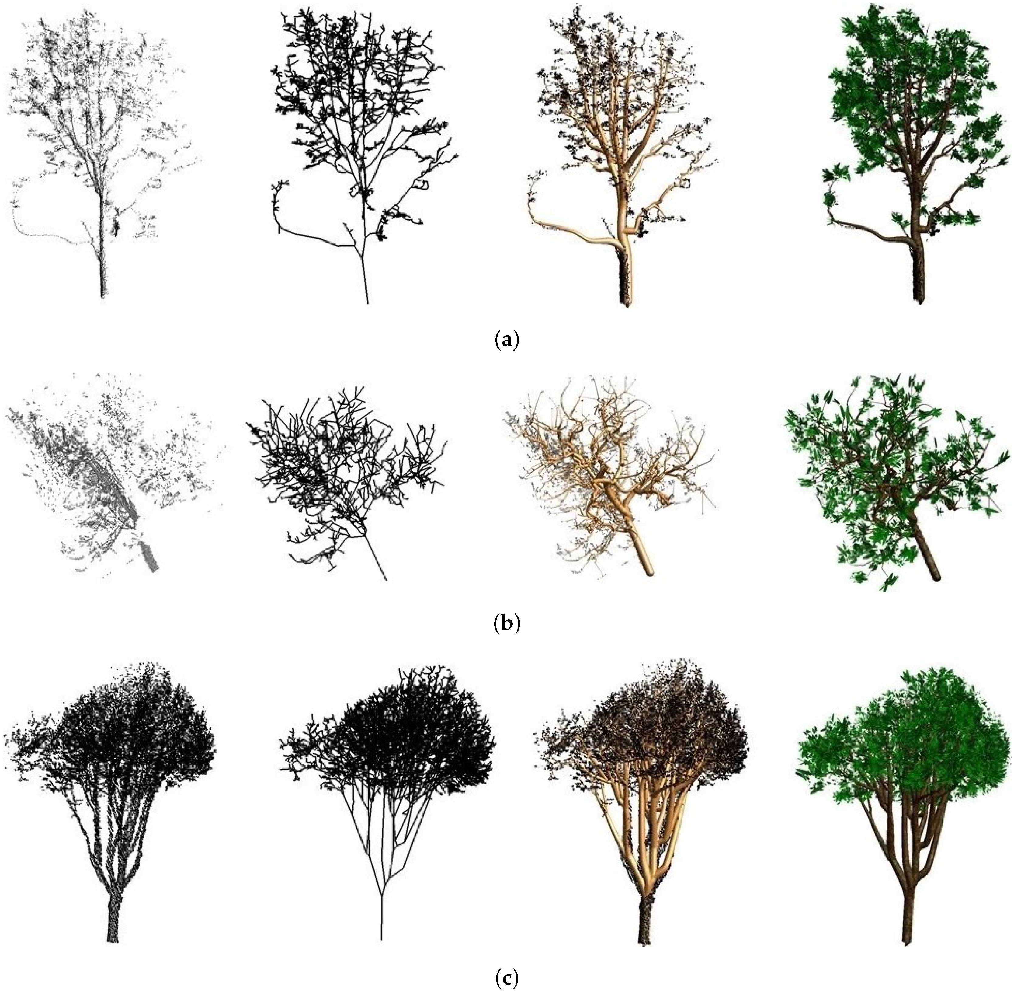
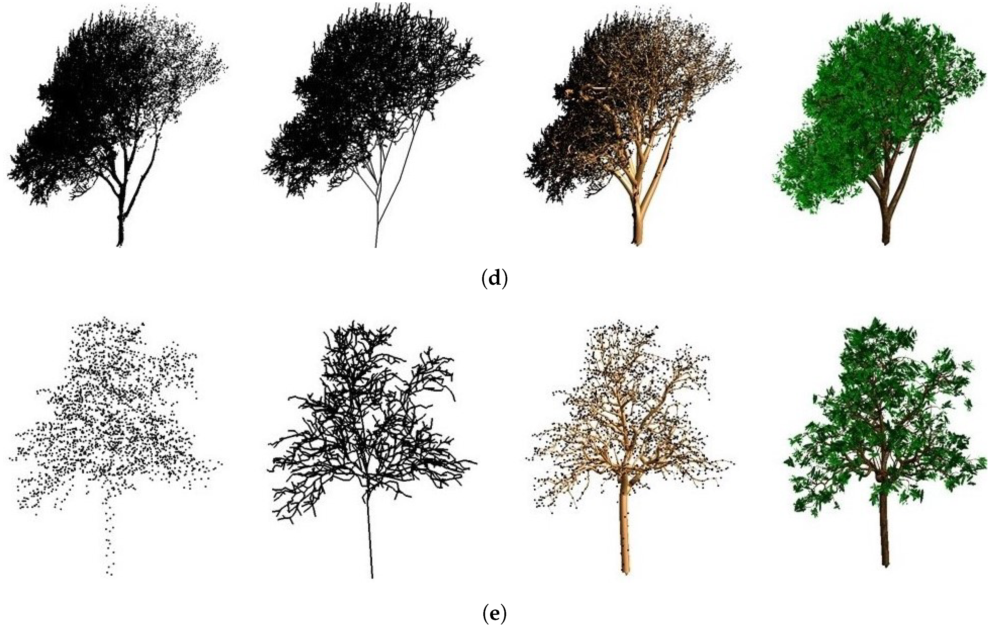
| Figure | Height (m) | Complexity | Point Number | Sensor Type | Accuracy (cm) | Stardard Deviation |
|---|---|---|---|---|---|---|
| Figure 11a | 5.52 | Medium | 11,855 | Mobile scanning | 2.76 | 2 |
| Figure 11b | 9.87 | Medium | 6992 | Mobile scanning | 10.04 | 8 |
| Figure 11c | 15.99 | Difficult | 28,993 | Mobile scanning | 6.59 | 6 |
| Figure 11d | 21.73 | Difficult | 137,407 | Static scanning | 6.50 | 6 |
| Figure 11e | 13.13 | Easy | 2488 | Airborne scanning | 11.88 | 7 |
© 2019 by the authors. Licensee MDPI, Basel, Switzerland. This article is an open access article distributed under the terms and conditions of the Creative Commons Attribution (CC BY) license (http://creativecommons.org/licenses/by/4.0/).
Share and Cite
Du, S.; Lindenbergh, R.; Ledoux, H.; Stoter, J.; Nan, L. AdTree: Accurate, Detailed, and Automatic Modelling of Laser-Scanned Trees. Remote Sens. 2019, 11, 2074. https://doi.org/10.3390/rs11182074
Du S, Lindenbergh R, Ledoux H, Stoter J, Nan L. AdTree: Accurate, Detailed, and Automatic Modelling of Laser-Scanned Trees. Remote Sensing. 2019; 11(18):2074. https://doi.org/10.3390/rs11182074
Chicago/Turabian StyleDu, Shenglan, Roderik Lindenbergh, Hugo Ledoux, Jantien Stoter, and Liangliang Nan. 2019. "AdTree: Accurate, Detailed, and Automatic Modelling of Laser-Scanned Trees" Remote Sensing 11, no. 18: 2074. https://doi.org/10.3390/rs11182074
APA StyleDu, S., Lindenbergh, R., Ledoux, H., Stoter, J., & Nan, L. (2019). AdTree: Accurate, Detailed, and Automatic Modelling of Laser-Scanned Trees. Remote Sensing, 11(18), 2074. https://doi.org/10.3390/rs11182074