Heterogeneous Behavior of the Campotosto Normal Fault (Central Italy) Imaged by InSAR GPS and Strong-Motion Data: Insights from the 18 January 2017 Events

 ,
,  , ,
, ,  , ,
, ,
Abstract

1. Introduction
2. Data
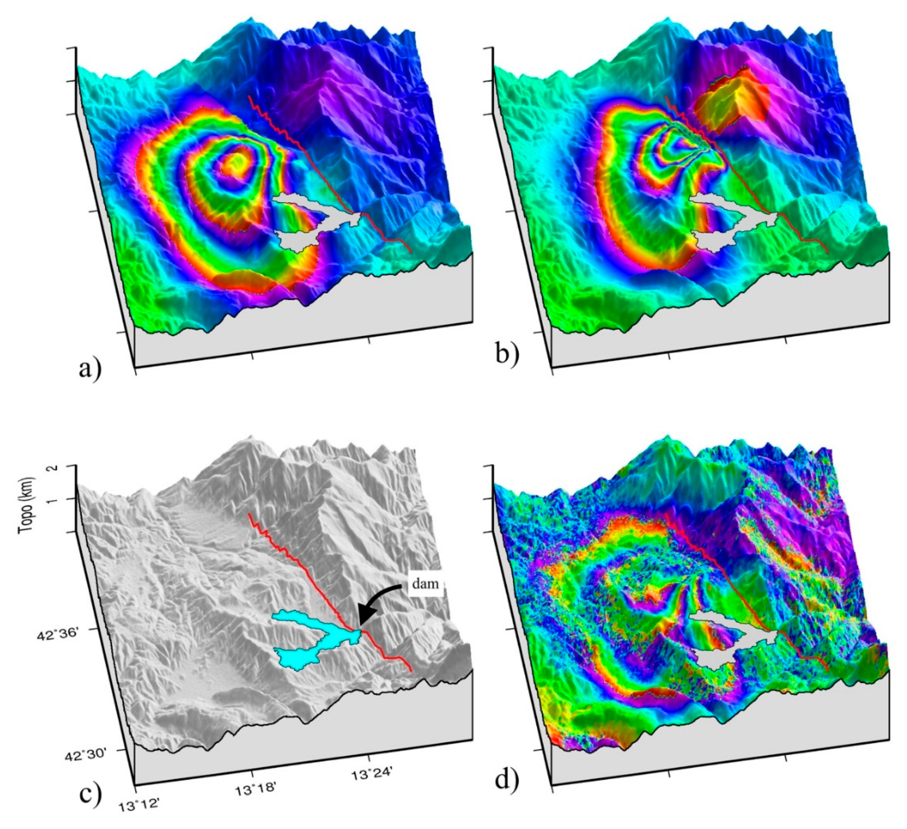
2.1. InSAR Data
2.2. GPS Static Offsets Data
2.3. Strong-Motion and High-Rate GPS Data
3. Inversion Results
3.1. Static Finite-Fault Modeling of the Cumulative Sequence
3.2. Testing the Vertical Continuity of the Campotosto Fault
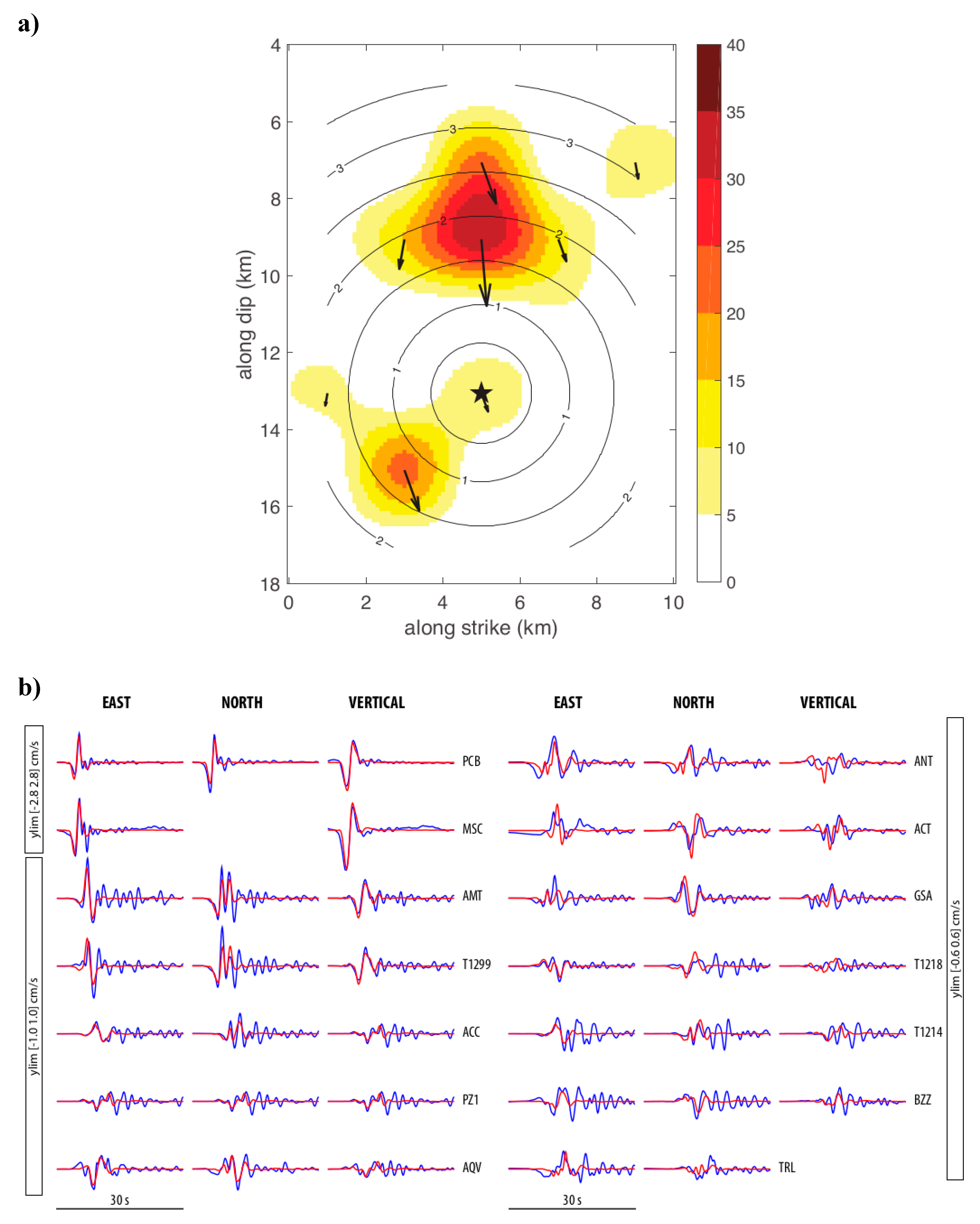
3.3. Kinematic Finite-Fault Slip Inversions of the Two Largest Events
3.3.1. The MW 5.5 Earthquake
3.3.2. The MW 5.4 Earthquake
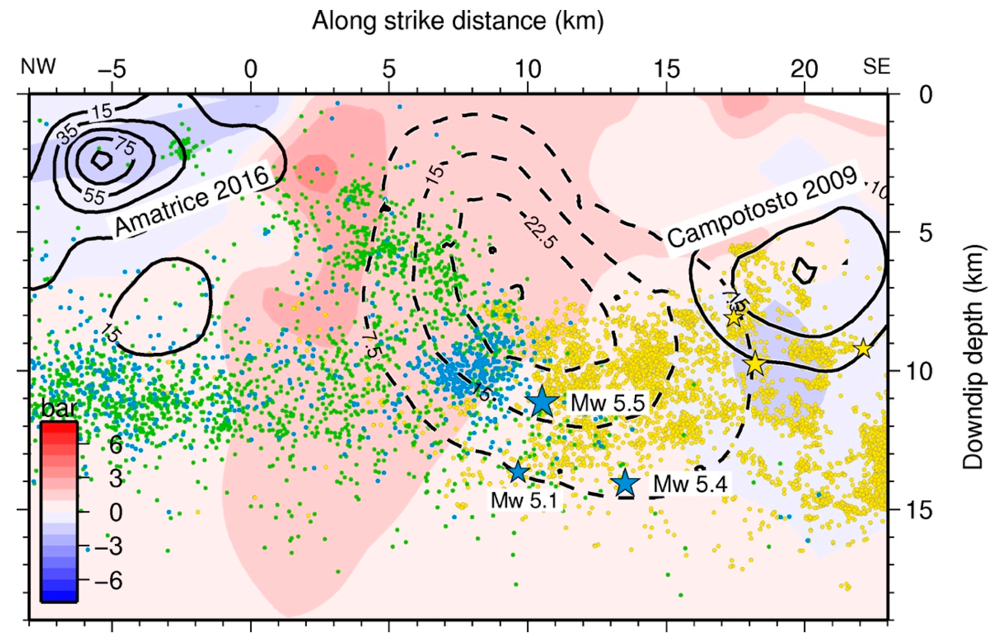
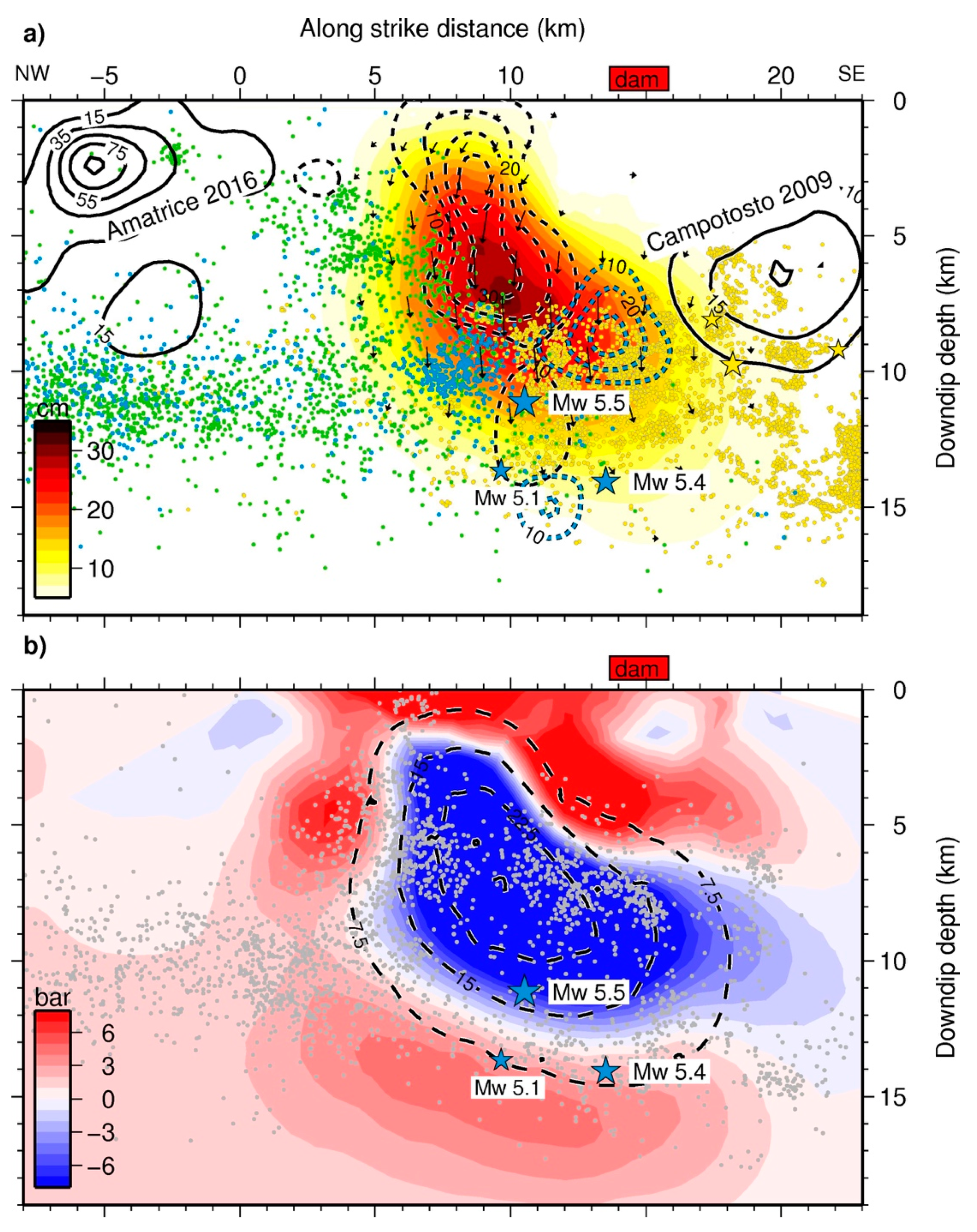
3.4. Static Coulomb Stress Change
4. Discussion
5. Conclusions
Supplementary Materials
Author Contributions
Funding
Acknowledgments
Conflicts of Interest
References
- Peng, Z.; Gomber, J. An integrated perspective of the continuum between earthquakes and slow-slip phenomena. Nat. Geosci. 2010, 3, 599–607. [Google Scholar] [CrossRef]
- Wei, S.; Helmberger, D.; Owen, S.; Graves, R.W.; Hudnut, K.W.; Fielding, E.J. Complementary slip distributions of the largest earthquakes in the 2012 Brawley swarm, Imperial Valley, California. Geophys. Res. Lett. 2013, 82, 847–852. [Google Scholar] [CrossRef]
- Avouac, J.-P. From geodetic imaging of seismic and aseismic fault slip to dynamic modeling of the seismic cycle. Annu. Rev. Earth Planet. Sci. 2015, 43, 233–271. [Google Scholar] [CrossRef]
- Villegas-Lanza, J.C.; Nocquet, J.-M.; Rolandone, F.; Vallée, M.; Tavera, H.; Bondoux, F.; Tran, T.; Martin, X.; Chlieh, M. A mixed seismic-aseismic stress release episode in the Andean subduction zone. Nat. Geosci. 2016, 9, 150–154. [Google Scholar] [CrossRef]
- Kyriakopoulos, C.; Chini, M.; Bignami, C.; Stramondo, S.; Ganas, A.; Kolligri, M.; Moshou, A. Monthly migration of a tectonic seismic swarm detected by DInSAR: Southwest Peloponnese, Greece. Geophys. J. Int. 2013, 194, 1302–1309. [Google Scholar] [CrossRef]
- Cheloni, D.; D’Agostino, N.; Selvaggi, G.; Avallone, A.; Fornaro, G.; Giuliani, R.; Reale, D.; Sansosti, E.; Tizzani, P. Aseismic transient during the 2010–2014 seismic swarm: Evidence for longer recurrence of M ≥ 6.5 earthquakes in the Pollino gap (Southern Italy)? Sci. Rep. 2017, 576, 1–10. [Google Scholar] [CrossRef]
- Gualandi, A.; Nichele, C.; Serpelloni, E.; Chiaraluce, L.; Anderlini, L.; Latorre, D.; Belardinelli, M.E.; Avouac, J.-P. Aseismic deformation associated with an earthquake swarm in the northern Apennines (Italy). Geophys. Res. Lett. 2017, 16, 7706–7714. [Google Scholar] [CrossRef]
- Page, M.; Felzer, K. Southern San Andreas Fault seismicity is consistent with the Gutunberg-Richter magnitude frequency distribution. Bull. Seismol. Soc. Am. 2015, 105, 2070–2080. [Google Scholar] [CrossRef]
- Parsons, T.; Geist, E.L. Is there basis for preferring characteristic earthquakes over Gutenberg-Richter distributions on individual faults in probabilistic earthquake forecasting? Bull. Seismol. Soc. Am. 2009, 99, 2012–2019. [Google Scholar] [CrossRef]
- Schwartz, D.P. Do large earthquakes on faults follow a Gutenberg-Richter or characteristic distribution? Seismol. Res. Lett. 2010, 81, 331. [Google Scholar]
- Chiaraluce, L.; Di Stefano, R.; Tinti, E.; Scognamiglio, L.; Michele, M.; Casarotti, E.; Cattaneo, M.; De Gori, P.; Chiarabba, C.; Monachesi, G.; et al. The 2016 Central Italy Seismic Sequence: A First Look at the Mainshocks, Aftershocks and Source Models. Seismol. Res. Lett. 2017, 88, 757–771. [Google Scholar] [CrossRef]
- Tinti, E.; Scognamiglio, L.; Michelini, A.; Cocco, M. Slip heterogeneity and directivity of the ML 6.0, 2016, Amatrice earthquake estimated with rapid finite-fault inversion. Geophys. Res. Lett. 2016, 43, 10745–10752. [Google Scholar] [CrossRef]
- Cheloni, D.; de Novellis, V.; Albano, M.; Antonioli, A.; Anzidei, M.; Atzori, S.; Avallone, A.; Bignami, C.; Bonano, M.; Calcaterra, S. Geodetic model of the 2016 Central Italy earthquake sequence inferred from InSAR and GPS data. Geophys. Res. Lett. 2017, 44, 6778–6787. [Google Scholar] [CrossRef]
- Walters, R.J.; Gregory, L.C.; Wedmore, L.N.J.; Craig, T.J.; McCaffrey, K.; Wilkinson, M.; Chen, J.; Li, Z.; Elliott, J.R.; Iezzi, H.; et al. Dual control of fault interactions on stop-start rupture in the 2016 Central Italy seismic sequence. Earth Planet. Sci. Lett. 2018, 500. [Google Scholar] [CrossRef]
- Cheloni, D.; Falcucci, E.; Gori, S. Half-graben rupture geometry of the 30 October 2016 Mw 6.6 Mt. Vettore-Mt. Bove earthquake, central Italy. J. Geophys. Res. 2019, 124. [Google Scholar] [CrossRef]
- Pizzi, A.; Di Domenica, A.; Gallovic, F.; Luzi, L.; Puglia, R. Fault Segmentation as Constraint to the Occurrence of the Main Shocks of the 2016 Central Italy Seismic Sequence. Tectonics 2017, 36. [Google Scholar] [CrossRef]
- Scognamiglio, L.; Tinti, E.; Casarotti, E.; Pucci, S.; Villani, F.; Cocco, M.; Magnoni, F.; Michelini, A.; Dreeger, D. Complex fault geometry and rupture dynamics of the MW 6.5, 2016, October 30th central Italy earthquake. J. Geophys. Res. 2018, 123. [Google Scholar] [CrossRef]
- Civico, R.; Pucci, S.; Villani, F.; Pizzimenti, L.; De Martini, P.M.; Nappi, R. The Open EMERGEo Working Group. Surface ruptures following the 30 October MW 6.5 Norcia earthquake, central Italy. J. Maps 2018, 14, 151–160. [Google Scholar] [CrossRef]
- Gori, S.; Falcucci, E.; Galadini, F.; Zimmaro, P.; Pizzi, A.; Kayen, R.E.; Lingwall, B.N.; Moro, M.; Saroli, M.; Fubelli, G.; et al. Surface Faulting Caused by the 2016 Central Italy Seismic Sequence: Field Mapping and LiDAR/UAV Imaging. Earthq. Spectra 2018, 34, 1585–1610. [Google Scholar] [CrossRef]
- Improta, L.; Latorre, D.; Margheriti, L.; Nardi, A.; Marchetti, A.; Lombardi, A.M.; Castello, B.; Villani, F.; Ciaccio, M.G.; Mele, F.M.; et al. Multi-segment rupture of the 2016 Amatrice-Visso-Norcia seismic sequence (central Italy) constrained by the first high-quality catalog of Early Aftershocks. Sci. Rep. 2019, 9, 6921. [Google Scholar] [CrossRef]
- Galadini, F.; Galli, P. Paleoseismology of silent faults in the Central Apennines (Italy): The Mt. Vettore and Laga Mts. faults. Ann. Geophys. 2003, 815–836. [Google Scholar] [CrossRef]
- Galli, P.; Galadini, F.; Pantosti, D. Twenty years of paleoseismology in Italy. Earth-Sci. Rev. 2008, 88, 89–117. [Google Scholar] [CrossRef]
- Blumetti, A.M.; Dramis, F.; Michetti, A.M. Fault-generated mountain fronts in the central Apennines (Central Italy): Geomorphological features and seismotectonic implications. Earth Surf. Proc. Land 1993, 18, 203–223. [Google Scholar] [CrossRef]
- Boncio, P.; Lavecchia, G.; Milana, G.; Rozzi, B. Seismogenesis in Central Apennines, Italy: An integrated analysis of minor earthquake sequences and structural data in the Amatrice-Campotosto area. Ann. Geophys. 2004, 47, 1723–1742. [Google Scholar] [CrossRef]
- Lavecchia, G.; Ferrarini, F.; Brozzetti, F.; De Nardis, R.; Boncio, P.; Chiaraluce, L. From surface geology to aftershock analysis: Constraints on the geometry of the L’Aquila 2009 seismogenic fault system. Ital. J. Geosci. 2012, 131, 330–347. [Google Scholar] [CrossRef]
- Falcucci, E.; Gori, S.; Galadini, F.; Fubelli, G.; Moro, M.; Saroli, M. Active faults in the epicentral and mesoseismal Ml 24, 2016 Amatrice earthquake region, central Italy. Methodological and seismotectonics issues. Ann. Geophys. 2016, 59. [Google Scholar] [CrossRef]
- Falcucci, E.; Gori, S.; Bignami, C.; Pietrantonio, G.; Melini, D.; Moro, M.; Saroli, M.; Galadini, F. The Campotosto Seismic Gap in Between the 2009 and 2016–2017 Seismic Sequences of Central Italy and the Role of Inherited Lithospheric Faults in Regional Seismotectonic Settings. Tectonics 2018, 37. [Google Scholar] [CrossRef]
- Boncio, P.; Lavecchia, G.; Pace, B. Defining model of 3D seismogenic sources for seismic hazard assessment applications: The case of central Apennines (Italy). J. Seismol. 2004, 8, 407–425. [Google Scholar] [CrossRef]
- Bigi, G.; Cosentino, D.; Parotto, M.; Sartoti, R.; Scandone, P. Structural Model of Italy, Scale 1:500.000; Consiglio Nazionale delle Ricerche: Rome, Italy, 1990; p. 193. [Google Scholar]
- Pizzi, A.; Galadini, F. Pre-existing cross-structure and active faults segmentation in the central Apennines (Italy). Tectonophysics 2009, 476. [Google Scholar] [CrossRef]
- Valoroso, L.; Chiaraluce, L.; Piccinini, D.; Di Stefano, R.; Schaff, D.; Waldhauser, F. Radiography of a normal fault system by 64,000 high-precision earthquake locations: The 2009 L’Aquila (central Italy) case study. J. Geophys. Res. 2013, 118, 1156–1176. [Google Scholar] [CrossRef]
- Chiarabba, C.; De Gori, P.; Catteneo, M.; Spallarossa, D.; Segou, M. Faults geometry and the role of fluids in the 2016–2017 Central Italy seismic sequence. Geophys. Res. Lett. 2018, 45, 6963–6971. [Google Scholar] [CrossRef]
- Rovida, A.; Locati, M.; Camassi, R.; Lolli, B.; Gasperini, P. CPTI15, the 2015 Version of the Parametric Catalogue of Italian Earthquakes; Istituto Nazionale di Geofisica e Vulcanologia: Roma, Italy, 2016. [Google Scholar] [CrossRef]
- Chiaraluce, L.; Valoroso, L.; Piccinini, D.; Di Stefano, R.; De Gori, P. Anatomy of the 2009 L’Aquila normal fault system (Central Italy) imaged by high resolution foreshock and aftershock locations. J. Geophys. Res. 2011, 116. [Google Scholar] [CrossRef]
- Malagnini, L.; Lucente, F.P.; De Gori, P.; Akinci, A.; Munafò, I. Control of pore fluid diffusion on fault failure mode: Insights from the 2009 L’Aquila seismic sequence. J. Geophys. Res. 2012, 117. [Google Scholar] [CrossRef]
- Cheloni, D.; Giuliani, R.; D’Anastasio, E.; Atzori, S.; Walters, R.J.; Bonci, L.; D’Agostino, N.; Mattone, M.; Calcaterra, S.; Gambino, P.; et al. Coseismic and post-seismic slip of the 2009 L’Aquila (central Italy) MW 6.3 earthquake and implications for seismic potential along the Campotosto fault from joint inversion of high-precision levelling, InSAR and GPS data. Tectonophysics 2014, 622, 168–185. [Google Scholar] [CrossRef]
- Xu, G.; Xu, C.; Wen, Y.; Jiang, G. Source Parameters of the 2016–2017 Central Italy Earthquake Sequence from the Sentinel-1, ALOS-2 and GPS Data. Remote Sens. 2017, 9, 1182. [Google Scholar] [CrossRef]
- D’Agostino, N. Complete seismic release of tectonics strain and earthquake recurrence in the Apennines (Italy). Geophys. Res. Lett. 2014, 41, 115–162. [Google Scholar] [CrossRef]
- Bigi, S.; Casero, P.; Chiarabba, C.; Di Bucci, D. Contrasting surface active faults and deep seismogenic sources unveiled by the 2009 L’Aquila earthquake sequence (Italy). Terra Nova 2012, 25. [Google Scholar] [CrossRef]
- Buttinelli, M.; Pezzo, G.; Valoroso, L.; De Gori, P.; Chiarabba, C. Tectonics Inversions, Fault Segmentations, and Triggering Mechanisms in the Central Apennines Normal Fault System: Insights from High-Resolution Velocity Models. Tectonics 2018, 37, 4135–4149. [Google Scholar] [CrossRef]
- Zebker, H.A.; Rosen, P.A.; Goldstein, R.M.; Gabriel, A.; Werner, C.L. On the derivation of coseismic displacement fields using differential radar interferometry: The Landers earthquake. J. Geophys. Res. 1994, 99, 19617–19634. [Google Scholar] [CrossRef]
- Farr, T.G.; Rosen, P.A.; Caro, E.; Crippen, R.; Duren, R.; Hensly, S.; Kobrik, M.; Paller, M.; Rodriguez, E.; Roth, L.; et al. The Shuttle Radar Topography Mission. Rev. Geophys. 2007, 45. [Google Scholar] [CrossRef]
- Goldstein, R.M.; Werner, C.L. Radar interferograms filtering for geophysical appplications. Geophys. Res. Lett. 1998, 25, 4035–4038. [Google Scholar] [CrossRef]
- Costantini, M. A novel phase unwrapping method based on network programming. IEEE Trans. Geosci. Remote Sens. 1998, 36, 813–821. [Google Scholar] [CrossRef]
- Surace, L. La nuova rete geodetica nazionale IGM95: Risultati e prospettive di utilizzazione. Boll. Geod. Sci. Affini 1997, 56, 358–378. [Google Scholar]
- Dach, R.; Hugentobler, U.; Fridez, P.; Meindl, M. Bernese GPS Software Version 5.0; Astronomical Institute, University of Bern: Bern, Switzerland, 2007. [Google Scholar]
- Bohm, J.; Niell, A.; Tregoning, P.; Schuh, H. Global Mapping Function (GMF): A new empirical mapping function based on numerical weather model data. Geophys. Res. Lett. 2006, 33. [Google Scholar] [CrossRef]
- Michelini, A.; Margheriti, L.; Cattaneo, M.; Cecere, G.; D’Anna, G.; Delladio, A.; Moretti, M.; Pintore, S.; Amato, A.; Basili, A.; et al. The Italian Seismic Network and the earthquake and tsunami monitoring and surveillance systems. Adv. Geosci. 2016, 43, 31–38. [Google Scholar] [CrossRef][Green Version]
- Moretti, M.; Pondrelli, S.; Margheriti, L.; Abruzzese, L.; Anselmi, M.; Arroucau, P.; Baccheschi, P.; Baptie, B.; Bonadio, R.; Bono, A.; et al. SISMIKO: Emergency network deployment and data sharing for the 2016 central Italy seismic sequence. Ann. Geophys. 2016, 59. [Google Scholar] [CrossRef]
- Bertiger, W.; Desai, S.D.; Haines, B.; Harvey, N.; Moore, A.W.; Owen, S.; Weiss, J.P. Single receiver phase ambiguity resolution with GPS data. J. Geod. 2010, 84, 327–337. [Google Scholar] [CrossRef]
- Avallone, A.; Latorre, D.; Serpelloni, E.; Cavaliere, A.; Herrero, A.; Cecere, G.; D’Agostino, N.; D’Ambrosio, C.; Devoti, R.; Giuliani, R.; et al. Coseismic displacement waveforms for the 2016 August 24 Mw 6.0 Amatrice earthquake (central Italy) carried out from High-Rate GPS data. Ann. Geophys. 2016, 59. [Google Scholar] [CrossRef]
- Choi, K.; Bilich, A.; Larson, K.M.; Axelrad, P. Modified sidereal filtering: Implications for high-rate GPS positioning. Geophys. Res. Lett. 2004, 31. [Google Scholar] [CrossRef]
- Widowinski, S.; Bock, Y.; Zhang, J.; Fang, P.; Genrich, J. Southern California permanent GPS geodetic array: Spatial filtering of daily positions for estimating coseismic and postseismic displacements induced by the 1992 Landers earthquake. J. Geophys. Res. 1987, 102, 18057–18070. [Google Scholar] [CrossRef]
- Okada, Y. Surface deformation due to shear and tensile faults in a half-space. Bull. Seism. Soc. Am. 1985, 75, 1135–1154. [Google Scholar]
- Cheloni, D.; D’Agostino, N.; D’Anastasio, E.; Avallone, A.; Mantenuto, S.; Giuliani, R.; Mattone, M.; Calcaterra, S.; Gambino, P.; Dominici, D.; et al. Coseismic and initial post-seismic slip of the 2009 MW 6.3 L’Aquila earthquake, Italy, from GPS measurements. Geophys. J. Int. 2010, 181, 1539–1546. [Google Scholar] [CrossRef]
- Avallone, A.; Cirella, A.; Cheloni, D.; Tolomei, C.; Theodoulidis, N.; Piatanesi, A.; Briole, P.; Ganas, A. Near-source high-rate GPS, strong motion and InSAR observations to image the 2015 Lefkada (Greece) Earthquake rupture history. Sci. Rep. 2018, 7. [Google Scholar] [CrossRef] [PubMed]
- Corana, A.; Marchesi, M.; Martini, C.; Ridella, S. Minimizing multimodal functions of continuous variables with the “Simulated Annealing” algorithm. ACM Trans. Math. Softw. 1987, 13, 262–280. [Google Scholar] [CrossRef]
- Press, W.H.; Teukolsky, S.A.; Vetterling, W.T.; Flannery, B.P. Numerical Recipes in C: The Art of Scientific Computing, 2nd ed.; Cambridge University Press: Cambridge, UK, 1992; pp. 262–280. [Google Scholar]
- Cheloni, D.; Giuliani, R.; D’Agostino, N.; Mattone, M.; Bonano, M.; Fornaro, G.; Lanari, R.; Reale, D.; Atzori, S. New insights into fault activation and stress transfer between en echelon thrusts: The 2012 Emilia, Northern Italy, earthquake sequence. J. Geophys. Res. 2016, 121. [Google Scholar] [CrossRef]
- Lohman, R.B.; Simons, M. Some thoughts on the use of InSAR data to constrain models of surface deformation: Noise structure and data downsampling. Geochem. Geophys. Geosyst. 2005, 6, Q01007. [Google Scholar] [CrossRef]
- Dreger, D.S.; Gee, L.; Lombard, P.; Murray, M.H.; Romanowicz, B. Rapid finite-source analysis and near-field strong ground motions: Application to the 2003 MW 6.5 San Simeon and 2004 MW 6.0 Parkfield earthquakes. Seismol. Res. Lett. 2005, 76, 40–48. [Google Scholar] [CrossRef]
- Herrmann, R.B.; Malagnini, L.; Munafò, I. Regional moment tensor of the 2009 L’Aquila earthquake sequence. Bull. Seismol. Soc. Am. 2011, 101, 975–993. [Google Scholar] [CrossRef]
- Lin, J.; Stein, R.S. Stress triggering in thrust and subduction earthquakes, and stress interaction between the southern San Andreas and nearby thrust and strike-slip faults. J. Geophys. Res. 2004, 109, B02303. [Google Scholar] [CrossRef]
- Perfettini, H.; Avouac, P. Modeling afterslip and aftershocks following the 1992 Landers earthquake. J. Geophys. Res. 2007, 112, B07409. [Google Scholar] [CrossRef]
- Hsu, Y.J.; Avouac, J.P.; Yu, S.B.; Chang, C.H.; Wu, Y.M.; Woessner, J. Spatio-temporal slip, and stress level on the faults within the western foothills of Taiwan: Implication for fault frictional properties. Pure Appl. Geophys. 2009, 166, 1853–1884. [Google Scholar] [CrossRef][Green Version]
- King, G.C.P.; Stein, R.S.; Lin, J. Static stress changes and the triggering of earthquakes. Bull. Seismol. Soc. Am. 1994, 84, 935–953. [Google Scholar]
- Freed, T.G. Earthquake triggering by static, dynamic, and post-seismic stress transfer. Annu. Rev. Earth Planet Sci. 2005, 33, 335–367. [Google Scholar] [CrossRef]
- Ryder, I.; Burgmann, R.; Fielding, E. Static stress interactions in extensional earthquake sequences: An example from the South Lunggar Rift, Tibet. J. Geophys. Res. 2012, 117. [Google Scholar] [CrossRef]
- Mildon, Z.K.; Roberts, G.P.; Faure Walker, J.P.; Iezzi, F. Coulomb stress transfer and fault interaction over millennia on non-planar active normal faults: The Mw 6.5-5.0 seismic sequence of 2016–2017, central Italy. Geophys. J. Int. 2017, 210, 1206–1218. [Google Scholar] [CrossRef]
- Boatwright, J.; Cocco, M. Frictional constraints on crustal faulting. J. Geophys. Res. 1996, 101, 13895–13909. [Google Scholar] [CrossRef]


© 2019 by the authors. Licensee MDPI, Basel, Switzerland. This article is an open access article distributed under the terms and conditions of the Creative Commons Attribution (CC BY) license (http://creativecommons.org/licenses/by/4.0/).
Share and Cite
Cheloni, D.; D’Agostino, N.; Scognamiglio, L.; Tinti, E.; Bignami, C.; Avallone, A.; Giuliani, R.; Calcaterra, S.; Gambino, P.; Mattone, M. Heterogeneous Behavior of the Campotosto Normal Fault (Central Italy) Imaged by InSAR GPS and Strong-Motion Data: Insights from the 18 January 2017 Events. Remote Sens. 2019, 11, 1482. https://doi.org/10.3390/rs11121482
Cheloni D, D’Agostino N, Scognamiglio L, Tinti E, Bignami C, Avallone A, Giuliani R, Calcaterra S, Gambino P, Mattone M. Heterogeneous Behavior of the Campotosto Normal Fault (Central Italy) Imaged by InSAR GPS and Strong-Motion Data: Insights from the 18 January 2017 Events. Remote Sensing. 2019; 11(12):1482. https://doi.org/10.3390/rs11121482
Chicago/Turabian StyleCheloni, Daniele, Nicola D’Agostino, Laura Scognamiglio, Elisa Tinti, Christian Bignami, Antonio Avallone, Roberta Giuliani, Stefano Calcaterra, Piera Gambino, and Maurizio Mattone. 2019. "Heterogeneous Behavior of the Campotosto Normal Fault (Central Italy) Imaged by InSAR GPS and Strong-Motion Data: Insights from the 18 January 2017 Events" Remote Sensing 11, no. 12: 1482. https://doi.org/10.3390/rs11121482
APA StyleCheloni, D., D’Agostino, N., Scognamiglio, L., Tinti, E., Bignami, C., Avallone, A., Giuliani, R., Calcaterra, S., Gambino, P., & Mattone, M. (2019). Heterogeneous Behavior of the Campotosto Normal Fault (Central Italy) Imaged by InSAR GPS and Strong-Motion Data: Insights from the 18 January 2017 Events. Remote Sensing, 11(12), 1482. https://doi.org/10.3390/rs11121482