Multi-Temporal Investigation of the Boulder Clay Glacier and Northern Foothills (Victoria Land, Antarctica) by Integrated Surveying Techniques


 , ,
, ,  , ,
, ,  ,
,
Abstract
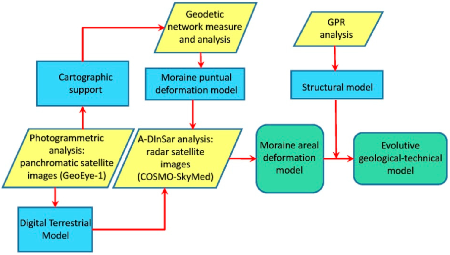
1. Introduction
- (i)
- Photogrammetry: to generate multi-temporal digital ortho-mosaics based both on available historical aerial images (1956, 1985, and 1993), and Very High Resolution (VHR) satellite stereo images acquired in 2012. Photogrammetry was applied even for the production of the reference map (high-resolution digital orthophoto), obtained through a photogrammetric process of stereopairs of satellite images using a set of Ground Control Points (GCPs) measured through a geodetic rapid-static GPS surveying technique. Data were integrated by a detailed Digital Terrain Model (DTM) of the BCG, obtained through a Terrestrial Laser Scanning (TLS) survey [9];
- (ii)
- Ground Penetrating Radar (GPR): to reveal the main bedrock morphology along the BCG area and to investigate the main supraglacial and subglacial features (water-collection areas, supraglacial and subglacial lakes, shear planes, crevasses), and the relationship between ice, moraine, and ice-cored debris in the Northern Foothills area;
- (iii)
- geodetic GPS network: to measure the horizontal and vertical rates of 12 station points specifically deployed in the runway embankment area. The network was measured five times, revealing different movement patterns of the moraine surface;
- (iv)
2. Boulder Clay Glacier Area Overview
3. Methods and Instrumentation
3.1. Photogrammetry
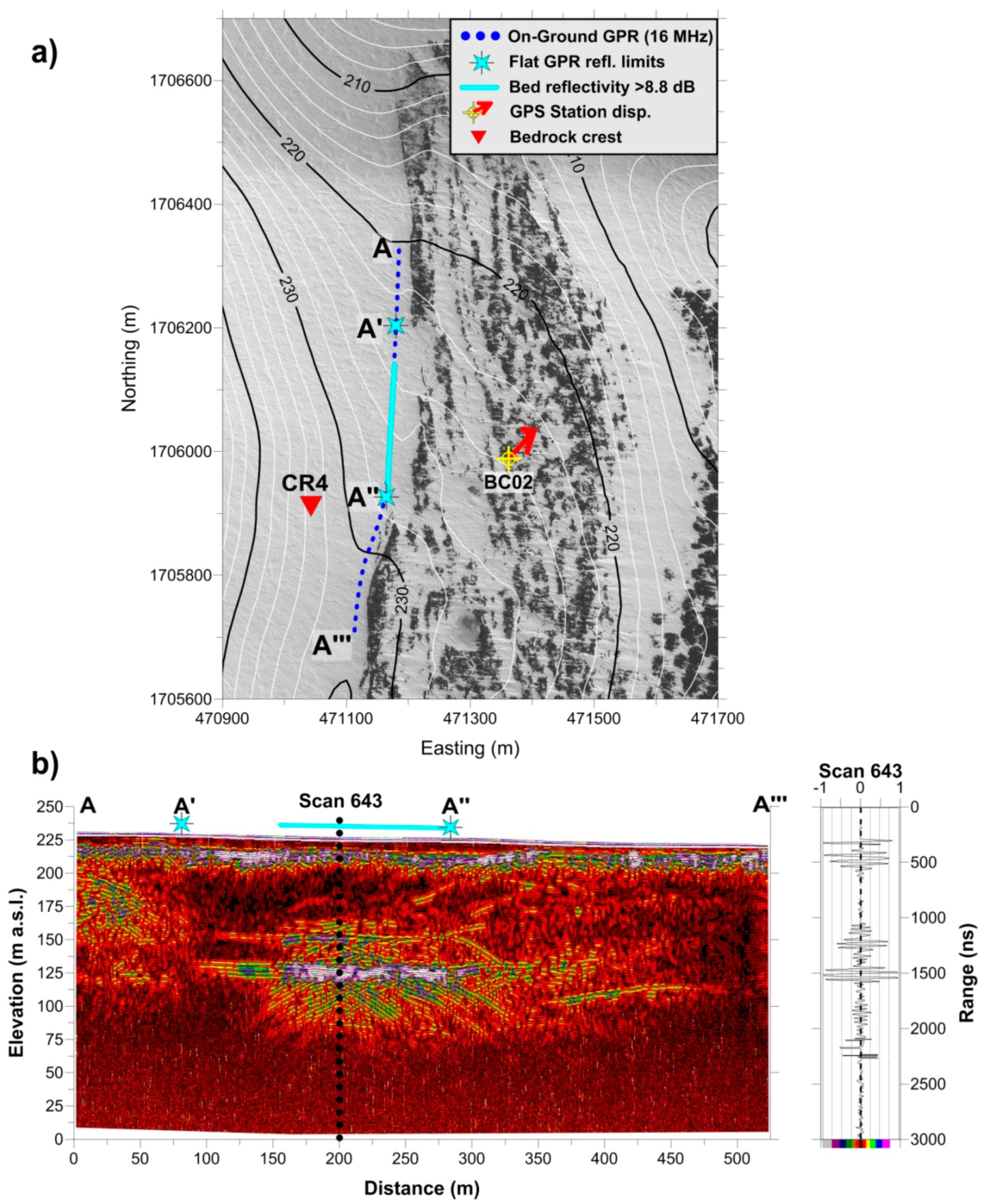
3.2. GPR Surveys
3.3. Geodetic GPS Network
3.4. InSAR Data Analysis
4. Results
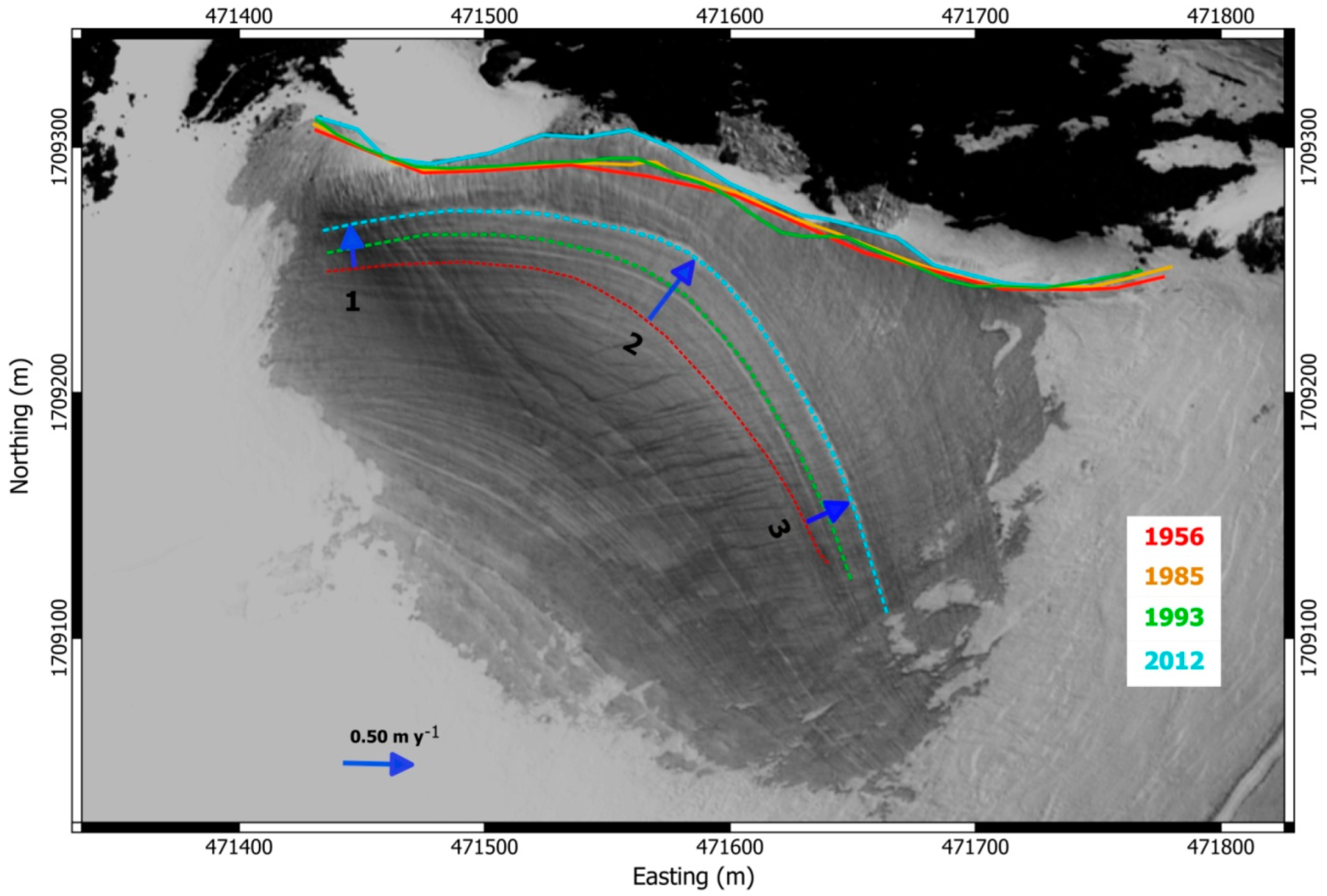
4.1. Comparison of Historical Photogrammetric Datasets
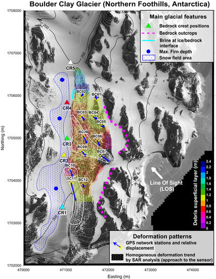
4.2. Boulder Clay Glacier Bedrock Structures
- (i)
- the glacier, fed by snow accumulation of lee-side snowfields;
- (ii)
- the ice-cored moraine, which is pushed eastward by the glacier toward a rising bedrock and under the influence of strong sublimation process induced by strong katabatic wind (up to 135 kn s−1, www.climantartide.it)
4.3. Glacier Features and Water/Brine Presence
4.4. Surface Displacements and Deformation Trends
- Bedrock outcrops: analysis did not show any detectable movements, so the points were used as reference during data processing (high signal stability);
- Glacier: the surface-displacement rate deducted from the analysis was up to 1 m y−1 in the higher slope area close two Adelie Cove along the low signal stability (LOS; Figure 12a,b);
- Moraine: characterized anomalous signal stability likely due to inhomogeneous surface dynamic (Figure 12c,d).
5. Discussion and Conclusions
- BCG moraine that is “relatively” stable, probably because it is an ice dead body, a relict of LGM marine ice sheet;
- Bedrock morphology and crests CR2 and CR4 that operate as “ice divides”, splitting up the ice flows;
- Ablation due to the strong katabatic winds blowing is the main process that allows the formation of BCG moraine;
- The presence of liquid brine at the ice/bedrock interface (Figure 11).
- The northern part: characterized by small or null movement;
- The centre part (between CR4 and CR2): it drains ice eastwardly, hosted and constrained in a funnel-shaped valley that seems to have only one narrow outlet to the right of BC07 station;
- The southern part (southward CR2): it drains ice toward Adelie Cove at a faster speed than the others, as also suggested by the topographic slope.
Supplementary Materials
Author Contributions
Funding
Acknowledgments
Conflicts of Interest
References
- Mellor, M. Notes on Antarctic Aviation. In CRREL Reports; Cold Regions Research and Engineering Laboratory: Hanover, NH, USA, 1993; pp. 14–93. [Google Scholar]
- Frezzotti, M. Ice front fluctuation, iceberg calving flux and mass balance of Victoria Land glaciers (Antarctica). Antarct. Sci. 1997, 9, 61–73. [Google Scholar] [CrossRef]
- Baroni, C.; Frezzotti, M.; Meneghel, M.; Orombelli, G.; Smiraglia, C.; Vittuari, L. Result of Monitoring of Local Glaciers at Terra Nova Bay (Victoria Land, Antarctica). Terra Antart. 1995, 2, 41–47. [Google Scholar]
- Frezzotti, M.; Capra, A.; Vittuari, L. Comparison between glacier ice velocities inferred from GPS and sequential satellite images. Ann. Glaciol. 1998, 27, 54–60. [Google Scholar] [CrossRef]
- Vittuari, L.; Vincent, C.; Frezzotti, M.; Mancini, F.; Gandolfi, S.; Bitelli, G.; Capra, A. Space geodesy as a tool for measuring ice surface velocity in the Dome C region and along ITASE traverse (East Antarctica). Ann. Glaciol. 2004, 39, 402–408. [Google Scholar] [CrossRef][Green Version]
- Winter, A.; Steinhage, D.; Arnold, E.J.; Blankenship, D.D.; Cavitte, M.G.P.; Corr, H.G.J.; Paden, J.D.; Urbini, S.; Young, D.A.; Eisen, O. Radio-echo sounding measurements and ice-core synchronization at Dome C, Antarctica. Cryosphere 2017, 11, 653–668. [Google Scholar] [CrossRef]
- Young, D.A.; Roberts, J.J.; Ritz, C.; Frezzotti, M.; Quartini, E.; Cavitte, M.G.P.; Tozer, C.R.; Steinhage, D.; Urbini, S.; Corr, H.F.J.; et al. High-resolution boundary conditions of an old ice target near Dome C, Antarctica. Cryosphere 2017, 11, 1897–1911. [Google Scholar] [CrossRef]
- Urbini, S.; Cafarella, L.; Tabacco, I.E.; Baskaradas, J.A.; Serafini, M.; Zirizzotti, A. RES Signatures of Ice Bottom Near to Dome C (Antarctica). IEEE Trans. Geosci. Remote Sens. 2015, 53, 1558–1564. [Google Scholar] [CrossRef]
- Abate, D.; Pierattini, S.; Bianchi-Fasani, G. Lidar in extreme environment: Surveying in Antarctica. In ISPRS Annals of the Photogrammetry, Remote Sensing and Spatial Information Sciences; Copernicus Publications: Göttingen, Germany, 2013; Volume II-5/W2. [Google Scholar]
- Goldstein, R.M.; Engelhardt, H.; Kamb, B.; Frolich, R.M. Satellite radar interferometry for monitoring ice sheet motion: Application to an Antarctic ice stream. Science 1993, 262, 1525–1530. [Google Scholar] [CrossRef]
- Rignot, E.; Mouginot, J.; Scheuchl, B. Ice flow of the Antarctic ice sheet. Science 2011, 333, 1427–1430. [Google Scholar] [CrossRef]
- Frezzotti, M.; Salvatore, M.C.; Vittuari, L.; Grigioni, P.; De Silvestri, L. Satellite Image Map: Northern Foothills and Inexpressible Island Area (Victoria Land, Antarctica); Terra Antartica Reports; Terra Antartica Publication: Siena, Italy, 2001; Volume 6, ISBN 8890022191. [Google Scholar]
- Stenni, B.; Serra, F.; Frezzotti, M.; Maggi, V.; Traversi, R.; Becagli, S.; Udisti, R. Snow accumulation rates in Northern Victoria Land (Antactica) by firn core analysis. J. Glaciol. 2000, 46, 541–552. [Google Scholar] [CrossRef]
- Chinn, T.J.H. Polar glacier margin and debris features. Memorie della Societa Geologica Italiana. In Proceedings of the Meeting on Earth Sciences in Antarctica, Saitama, Japan, 9–13 September 1991; Volume 46, pp. 25–44. [Google Scholar]
- Baroni, C. Geomorphological map of the Northern Foothills near the Italian station (Terra Nova Bay, Antarctica). Mem. Della Soc. Geol. Ital. 1987, XXXIII, 195–212. [Google Scholar]
- Baroni, C.; Orombelli, G. Glacial geology and geomorphology of Terra Nova Bay (Victoria Land, Antarctica). Mem. Della Soc. Geol. Ital. 1987, XXXIII, 171–194. [Google Scholar]
- Guglielmin, M. Ground Surface Temperature (GST), Active Layer and Permafrost monitoring in Continental Antarctica. Permafr. Periglac. Process. 2006, 17, 133–143. [Google Scholar] [CrossRef]
- Raffi, R.; Stenni, B.; Flora, O.; Polesello, S.; Camusso, M. Growth processes of an inland Antarctic ice wedge, Mesa Range, northern Victoria Land. Ann. Glaciol. 2004, 39, 1–8. [Google Scholar] [CrossRef]
- Atkins, C. Geomorphological evidence of cold-based glacier activity in South Victoria Land, Antarctica. Geol. Soc. Lond. Spec. Publ. 2013, 381, 299–318. [Google Scholar] [CrossRef]
- Nye, J.F. The mechanics of glacier flow. J. Glaciol. 1952, 2, 82–93. [Google Scholar] [CrossRef]
- Chinn, T.J.H. Glacial History and Glaciology of Terra Nova Bay Area; Logistic Report for K162; Report n. WS 998; Water and Soil Centre: Christchurch, New Zealand, 1985. [Google Scholar]
- Denton, G.H.; Borns, H.W.J.; Grosswald, M.G.; Stuiver, M.; Nichols, R.L. Glacial history of the Ross Sea. Antarct. J. U.S. 1975, 10, 160–164. [Google Scholar]
- Orombelli, G. La prima Spedizione del Programma Nazionale di Ricerche in Antartide. Osservazioni geomorfologiche. Riv. Geograf. Ital. 1986, 93, 129–169. [Google Scholar]
- Orombelli, G.; Baroni, C.; Denton, G.H. Late Cenozoic glacial history of the Terra Nova Bay region, Northern Victoria Land, Antarctica. Geogr. Fis. Din. Quat. 1990, 13, 139–163. [Google Scholar]
- Chinn, T.J.H. Physical hydrology of the Dry Valley Lakes. In Physical and Biogeochemical Processes in Antarctic Lakes. Antarctic Research Series; Green, W.J., Friedmann, E.I., Eds.; American Geophysical Union: Washington, DC, USA, 1993; Volume 59, pp. 1–51. [Google Scholar]
- French, H.M.; Guglielmin, M. Frozen ground phenomena in the vicinity of Terra Nova Bay, Northern Victoria Land, Antarctica: A preliminary report. Geogr. Ann. 2000, 82, 513–526. [Google Scholar] [CrossRef]
- French, H.M. The Periglacial Environment, 3rd ed.; John Wiley & Sons Limited: Chichester, UK, 2007; Volume 458. [Google Scholar]
- Guglielmin, M.; Lewkovicz, A.G.; French, M.F.; Strini, A. Lake-ice blisters, Terra Nova Bay Area, Northern Victoria Land, Antarctica. Geogr. Ann. 2009, 91, 99–111. [Google Scholar] [CrossRef]
- Ullman, S. The interpretation of structure from motion. Proc. R. Soc. Lond. Ser. B Biol. Sci. 1979, 203, 405–426. [Google Scholar] [CrossRef]
- Seitz, S.; Snavely, N.; Szeliski, R. Photo tourism: Exploring photo collections in 3D. ACM Trans. Graph. 2006, 25, 835–846. [Google Scholar] [CrossRef]
- Zanutta, A.; Baldi, P.; Bitelli, G.; Cardinali, M.; Carrara, A. Qualitative and quantitative photogrammetric techniques for multi-temporal landslide analysis. Ann. Glaciol. 2006, 49, 1067–1079. [Google Scholar] [CrossRef]
- D’Agata, C.; Zanutta, A. Reconstruction of the recent changes of a debris covered glacier (Brenva, Mont Blanc Massif, Italy) using indirect source: Methods, results and validation. Glob. Planet. Chang. 2007, 56, 1–2. [Google Scholar] [CrossRef]
- Glen, J.W.; Paren, J.G. The electrical properties of snow and ice. J. Glaciol. 1975, 15, 15–38. [Google Scholar] [CrossRef]
- Bogorosky, V.V.; Benteley, C.R.; Gudmandsen, P.E. Radioglaciology, Glaciology and Quaternary Geology; Springer: Dordrecht, The Netherlands, 1985; Volume 1, p. 272. [Google Scholar]
- Herring, T. MATLAB Tools for viewing GPS velocities and time series. GPS Solut. 2003, 7, 194–199. [Google Scholar] [CrossRef]
- Perissin, D.; Wang, Z.; Wang, T. SARPROZ InSAR Tool for Urban Subsidence/manmade Structure Stability Monitoring in China. In Proceedings of the ISRSE 2011, Sidney, Australia, 10–15 April 2011. [Google Scholar]
- Perissin, D.; Wang, T. Repeat-Pass SAR Interferometry with Partially Coherent Targets. IEEE Trans. Geosci. Remote Sens. 2012, 50, 271–280. [Google Scholar] [CrossRef]
- Gandolfi, S.; Meneghel, M.; Salvatore, M.C.; Vittuari, L. Kinematic global positioning system to monitor small Antarctic glaciers. Ann. Glaciol. 1997, 24, 326–330. [Google Scholar] [CrossRef][Green Version]
- Bondesan, A.; Meneghel, M.; Salvatore, M.C. Local glacier snout monitoring in Northern Victoria Land, Antarctica; Terra Antartica Reports; Terra Antartica Publication: Siena, Italy, 2003; Volume 8, pp. 1–4. ISBN 88-88395-02-4. [Google Scholar]
- Diolaiuti, G.; Smiraglia, C.; Vassena, G.; Motta, M. Dry calving processes at the ice cliff of Strandline Glacier northern Victoria Land, Antarctica. Ann. Glaciol. 2004, 39, 201–208. [Google Scholar] [CrossRef][Green Version]
- Orombelli, G. Holocene environmental changes at Terra Nova Bay (Victoria Land, Antarctica). Mem. Soc. Geol. Ital. 1990, 34, 159–162. [Google Scholar]
- Rocchi, S.; Di Vincenzo, G.; Ghezzo, C. The Terra Nova Intrusive Complex, Victoria Land, Antarctica (with 1:50,000 geopetrographic map); Terra Antartica Reports; Terra Antartica Publication: Siena, Italy, 2004; Volume 10, pp. 1–51. ISBN 88-88395-07-5. [Google Scholar]
- French, H.M.; Guglielmin, M. Observations on the ice-marginal, periglacial geomorphology of Terra Nova Bay, Northern Victoria Land, Antarctica. Permafr. Periglac. Process. 1999, 10, 331–347. [Google Scholar] [CrossRef]
- Zirizzotti, A.; Cafarella, L.; Urbini, S. Ice and bedrock characteristics underneath Dome C (Antarctica) from RES data analysis. IEEE Trans. Geosci. Remote Sens. 2011, 50, 37–43. [Google Scholar] [CrossRef]
- Badgeley, J.A.; Pettit, E.C.; Carr, C.G.; Tulaczyk, S.; Mikucki, J.A.; Lyons, W.B.; MIDGE Science Team. An englacial hydrologic system of brine within a cold glacier: Blood Falls, McMurdo Dry Valleys, Antarctica. J. Glaciol. 2017, 63, 387–400. [Google Scholar] [CrossRef]
- Rutishauser, A.; Blankenship, D.D.; Sharp, M.; Skidmore, M.L.; Greenbaum, J.S.; Grima, C.; Schroeder, D.M.; Young, D.A. Discovery of a hypersaline subglacial lake complex beneath Devon Ice Cap, Canadian Arctic. Sci. Adv. 2018, 4, eaar4353. [Google Scholar] [CrossRef]
- Lyons, B.W.; Mikucki, J.A.; German, L.A.; Welch, K.A.; Welch, S.A.; Gardner, C.B.; Tulaczyk, S.M.; Pettit, E.C.; Kowalski, J.; Dachwald, B.; et al. The Geochemistry of Englacial Brine from Taylor Glacier, Antarctica. J. Geophys. Res. 2019, 124. [Google Scholar] [CrossRef]
- Yang, J.W.; Han, Y.; Orsi, A.J.; Kim, S.J.; Han, H.; Jang, Y.R.Y.; Moon, J.; Choi, T.; Hur, S.D.; Ahn, J. Surface temperature in twentieth century at the Styx Glacier, northern Victoria Land, Antarctica, from borehole thermometry. Geophys. Res. Lett. 2018, 45, 9834–9842. [Google Scholar] [CrossRef]


| Date | N. of Images | Focal Length (mm) | Altitude (feet) | Scale | Scanning Resolution (μm) | Ground Sampling Distance (m) |
|---|---|---|---|---|---|---|
| Dec. 1956 | 7 | 154.19 | 16,000 | 1:32,000 | 9 | 0.28 |
| Nov. 1985 | 6 | 152.27 | 28,000 | 1:56,000 | 25 | 1.4 |
| Nov. 1993 | 6 | 152.85 | 11,800 | 1:24,000 | 13.5 | 0.32 |
| DATASET A | DATASET B | ||||||
|---|---|---|---|---|---|---|---|
| Satellite | Date | Orbit N° | Bn (m) | Satellite | Date | Orbit N° | Bn (m) |
| SAR2 | 25 February 2013 | 28,218 | 346 | SAR2 | 11 January 2014 | 32,958 | 792 |
| SAR3 | 26 February 13 | 23,478 | 339 | SAR4 | 15 January 14 | 17,272 | 854 |
| SAR4 | 1 March 13 | 12,532 | 231 | SAR1 | 19 January 14 | 35,802 | 645 |
| SAR1 | 5 March 13 | 31,062 | 302 | SAR2 | 27 January 14 | 33,195 | 584 |
| SAR2 | 13 March 13 | 28,455 | 360 | SAR4 | 31 January 14 | 17,509 | 650 |
| SAR3 | 14 March 13 | 23,715 | 228 | SAR1 | 4 February 14 | 36,039 | 511 |
| SAR1 | 21 March 13 | 31,299 | 247 | SAR2 | 12 February 14 | 33,432 | 506 |
| SAR2 | 29 March 13 | 28,692 | 153 | SAR4 | 16 February 14 | 17,746 | 612 |
| SAR3 | 30 March 13 | 23,952 | 239 | SAR1 | 20 February 14 | 36,276 | 368 |
| SAR4 | 2 April 13 | 13,006 | 70 | SAR2 | 28 February 14 | 33,669 | 480 |
| SAR1 | 6 April 13 | 31,536 | −25 | SAR4 | 4 March 14 | 17,983 | 457 |
| SAR2 | 14 April 13 | 28,929 | 78 | SAR1 | 8 March 14 | 36,513 | 381 |
| SAR4 | 18 April 13 | 13,243 | −21 | SAR2 | 16 March 14 | 33,906 | 332 |
| SAR1 | 22 April 13 | 31,773 | −21 | SAR4 | 20 March 14 | 18,220 | 292 |
| SAR2 | 30 April 13 | 29,166 | 75 | SAR1 | 24 March 14 | 36,750 | 210 |
| SAR3 | 17 May 13 | 24,663 | −38 | SAR2 | 1 April 14 | 34,143 | 360 |
| SAR4 | 20 May 13 | 13,717 | 11 | SAR4 | 5 April 14 | 18,457 | 299 |
| SAR1 | 24 May 13 | 32,247 | 156 | SAR2 | 17 April 14 | 34,380 | 278 |
| SAR2 | 17 June 13 | 29,877 | 36 | SAR4 | 21 April 14 | 18,694 | 263 |
| SAR3 | 18 June 13 | 25,137 | 105 | SAR1 | 25 April 14 | 37,224 | 334 |
| SAR2 | 3 July 13 | 30,114 | 25 | SAR2 | 3 May 14 | 34,617 | 316 |
| SAR3 | 4 July 13 | 25,374 | 50 | SAR4 | 7 May 14 | 18,931 | 46 |
| SAR4 | 7 July 13 | 14,428 | 129 | SAR1 | 11 May 14 | 37,461 | 91 |
| SAR2 | 19 July 13 | 30,351 | 12 | SAR2 | 19 May 14 | 34,854 | 0 |
| SAR3 | 20 July 13 | 25,611 | 85 | SAR1 | 27 May 14 | 37,698 | 80 |
| SAR4 | 23 July 13 | 14,665 | 0 | SAR1 | 12 June 14 | 37,935 | 11 |
| SAR1 | 27 July 13 | 33,195 | −196 | SAR2 | 20 June 14 | 35,328 | −52 |
| SAR2 | 4 August 13 | 30,588 | 23 | SAR1 | 28 June 14 | 38,172 | 38 |
| SAR3 | 5 August 13 | 25,848 | 30 | SAR1 | 14 July 14 | 38,409 | 117 |
| SAR4 | 8 August 13 | 14,902 | −69 | SAR2 | 22 July 14 | 35,802 | 11 |
| SAR1 | 12 August 13 | 33,432 | −53 | SAR1 | 30 July 14 | 38,646 | 58 |
| SAR2 | 20 August 13 | 30,825 | −105 | SAR2 | 7 August 14 | 36,039 | −49 |
| SAR3 | 21 August 13 | 26,085 | −54 | SAR1 | 15 August 14 | 38,883 | −65 |
| SAR4 | 24 August 13 | 15,139 | −154 | SAR2 | 23 August 14 | 36,276 | −4 |
| SAR1 | 28 August 13 | 33,669 | −107 | SAR4 | 27 August 14 | 20,590 | 23 |
| SAR2 | 5 September 13 | 31,062 | −120 | SAR1 | 31 August 14 | 39,120 | 7 |
| SAR3 | 6 September 13 | 26,322 | −104 | SAR2 | 8 September 14 | 36,513 | 2 |
| SAR1 | 13 September 13 | 33,906 | −205 | SAR4 | 12 September 14 | 20,827 | −15 |
| SAR3 | 22 September 13 | 26,559 | −31 | SAR1 | 16 September 14 | 39,357 | −88 |
| SAR4 | 25 September 13 | 15,613 | −105 | SAR2 | 24 September 14 | 36,750 | −27 |
| SAR1 | 29 September 13 | 34,143 | 47 | SAR4 | 28 September 14 | 21,064 | −62 |
| SAR2 | 7 October 13 | 31,536 | 15 | SAR1 | 2 October 14 | 39,594 | −16 |
| SAR3 | 8 October 13 | 26,796 | −32 | SAR2 | 10 October 14 | 36,987 | 64 |
| SAR4 | 11 October 13 | 15,850 | −3 | SAR4 | 30 October 14 | 21,538 | 134 |
| SAR1 | 15 October 13 | 34,380 | −10 | SAR1 | 3 November 14 | 40,068 | 265 |
| SAR2 | 23 October 13 | 31,773 | 94 | SAR2 | 11 November 14 | 37,461 | 166 |
| SAR1 | 31 October 13 | 34,617 | 101 | SAR4 | 15 November 14 | 21,775 | 265 |
| SAR2 | 8 November 13 | 32,010 | 153 | SAR2 | 27 November 14 | 37,698 | 379 |
| SAR1 | 16 November 13 | 34,854 | 279 | SAR4 | 1 December 14 | 22,012 | 280 |
| SAR2 | 24 November 13 | 32,247 | 15 | ||||
| SAR4 | 28 November 13 | 16,561 | 76 | ||||
| SAR2 | 10 December 13 | 32,484 | 259 | ||||
| Ice Velocity Point | 1956–1993 m y−1 | 1993–2012 m y−1 | 1956–2012 m y−1 |
|---|---|---|---|
| 1 | 0.22 ± 0.14 | 0.51 ± 0.2 | 0.32 ± 0.07 |
| 2 | 0.47 ± 0.14 | 0.8 ± 0.2 | 0.59 ± 0.07 |
| 3 | 0.26 ± 0.14 | 0.57 ± 0.2 | 0.36 ± 0.07 |
| Parameters | Value |
|---|---|
| Dissolved oxygen (mg/L) | 0.28 |
| pH | 9.00 |
| Temperature (°C) | 0.14 |
| Resistivity (MΩ/cm) | 0.0002 |
| Conductivity (µS/cm) | 4091 |
| Total dissolved solids (ppm) | 2045 |
| Salinity (%) | 2.13 |
| Oxidation-reduction potential | −154.4 |
| GPS | VNorth | VEast | VUP | VHorizontal | Azimut |
|---|---|---|---|---|---|
| Stations | (mm y−1) | (mm y−1) | (mm y−1) | (mm y−1) | (°) |
| BC01 | 1.50 ± 0.69 | −1.02 ± 0.75 | 0.64 ± 1.68 | 1.81 ± 1.02 | 326 |
| BC02 | 1.97 ± 0.48 | 4.33 ± 0.28 | 4.76 ± 0.71 | 4.76 ± 0.56 | 66 |
| BC03 | −4.01 ± 0.28 | 7.34 ± 0.25 | 1.02 ± 1.54 | 8.36 ± 0.37 | 119 |
| BC04 | −2.43 ± 0.84 | 10.88 ± 2.70 | −4.43 ± 0.95 | 11.15 ± 2.83 | 103 |
| BC05 | −0.32 ± 0.79 | 9.50 ± 1.05 | −0.63 ± 1.50 | 9.50 ± 1.31 | 92 |
| BC06 | −7.21 ± 0.69 | 8.49 ± 1.52 | −2.63 ± 1.45 | 11.14 ± 1.67 | 130 |
| BC07 | −8.70 ± 1.05 | 30.53 ± 2.18 | 1.48 ± 2.79 | 31.74 ± 2.42 | 106 |
| BC08 | −10.06 ± 1.50 | 13.86 ± 1.50 | 3.99 ± 2.14 | 17.13 ± 2.12 | 126 |
| BC09 | −7.27 ± 1.18 | 14.92 ± 1.30 | 2.49 ± 2.51 | 16.60 ± 1.76 | 116 |
| BC10 | −9.17 ± 1.48 | 8.51 ± 0.69 | 4.26 ± 2.62 | 12.51 ± 1.63 | 137 |
| BC11 | −32.49 ± 0.32 | 20.97 ± 1.30 | 1.85 ± 2.57 | 38.67 ± 1.34 | 147 |
| BC12 | −1.45 ± 0.44 | 1.09 ± 0.35 | 2.68 ± 1.37 | 1.81 ± 0.56 | 143 |
© 2019 by the authors. Licensee MDPI, Basel, Switzerland. This article is an open access article distributed under the terms and conditions of the Creative Commons Attribution (CC BY) license (http://creativecommons.org/licenses/by/4.0/).
Share and Cite
Urbini, S.; Bianchi-Fasani, G.; Mazzanti, P.; Rocca, A.; Vittuari, L.; Zanutta, A.; Girelli, V.A.; Serafini, M.; Zirizzotti, A.; Frezzotti, M. Multi-Temporal Investigation of the Boulder Clay Glacier and Northern Foothills (Victoria Land, Antarctica) by Integrated Surveying Techniques. Remote Sens. 2019, 11, 1501. https://doi.org/10.3390/rs11121501
Urbini S, Bianchi-Fasani G, Mazzanti P, Rocca A, Vittuari L, Zanutta A, Girelli VA, Serafini M, Zirizzotti A, Frezzotti M. Multi-Temporal Investigation of the Boulder Clay Glacier and Northern Foothills (Victoria Land, Antarctica) by Integrated Surveying Techniques. Remote Sensing. 2019; 11(12):1501. https://doi.org/10.3390/rs11121501
Chicago/Turabian StyleUrbini, Stefano, Gianluca Bianchi-Fasani, Paolo Mazzanti, Alfredo Rocca, Luca Vittuari, Antonio Zanutta, Valentina Alena Girelli, Michelina Serafini, Achille Zirizzotti, and Massimo Frezzotti. 2019. "Multi-Temporal Investigation of the Boulder Clay Glacier and Northern Foothills (Victoria Land, Antarctica) by Integrated Surveying Techniques" Remote Sensing 11, no. 12: 1501. https://doi.org/10.3390/rs11121501
APA StyleUrbini, S., Bianchi-Fasani, G., Mazzanti, P., Rocca, A., Vittuari, L., Zanutta, A., Girelli, V. A., Serafini, M., Zirizzotti, A., & Frezzotti, M. (2019). Multi-Temporal Investigation of the Boulder Clay Glacier and Northern Foothills (Victoria Land, Antarctica) by Integrated Surveying Techniques. Remote Sensing, 11(12), 1501. https://doi.org/10.3390/rs11121501