A New Fast and Low-Cost Photogrammetry Method for the Engineering Characterization of Rock Slopes


 ,
,
Abstract

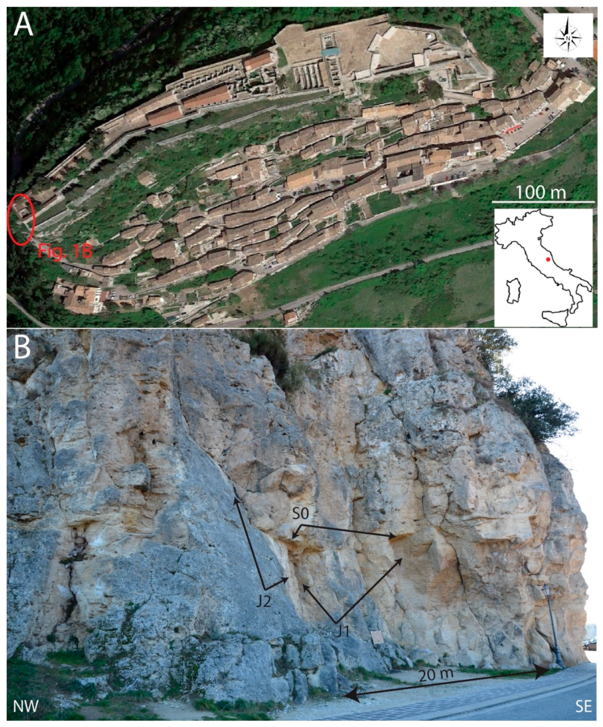
1. Introduction
2. Materials and Methods
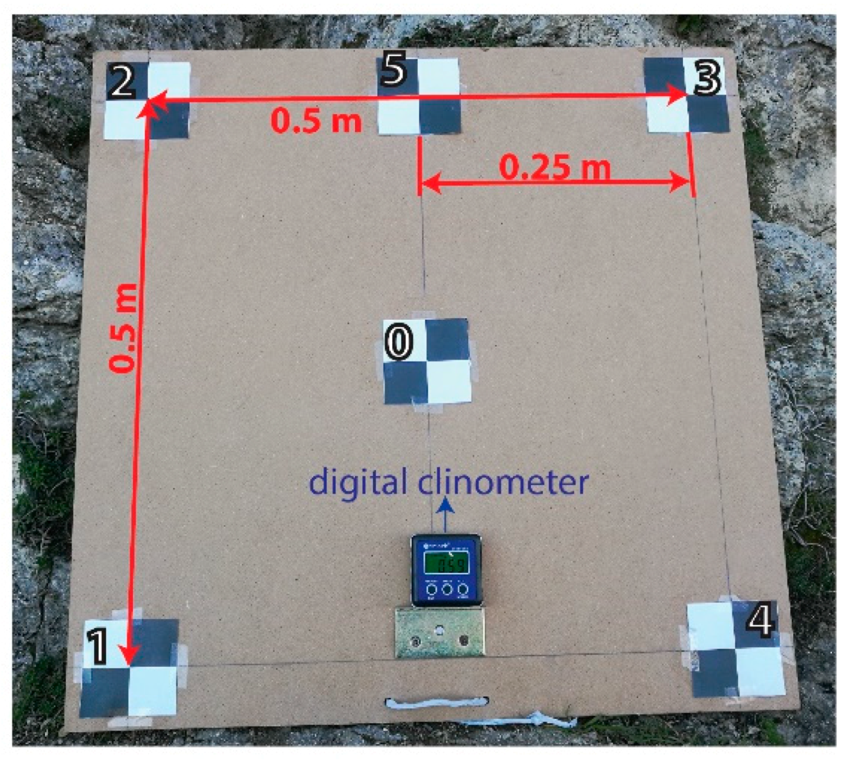
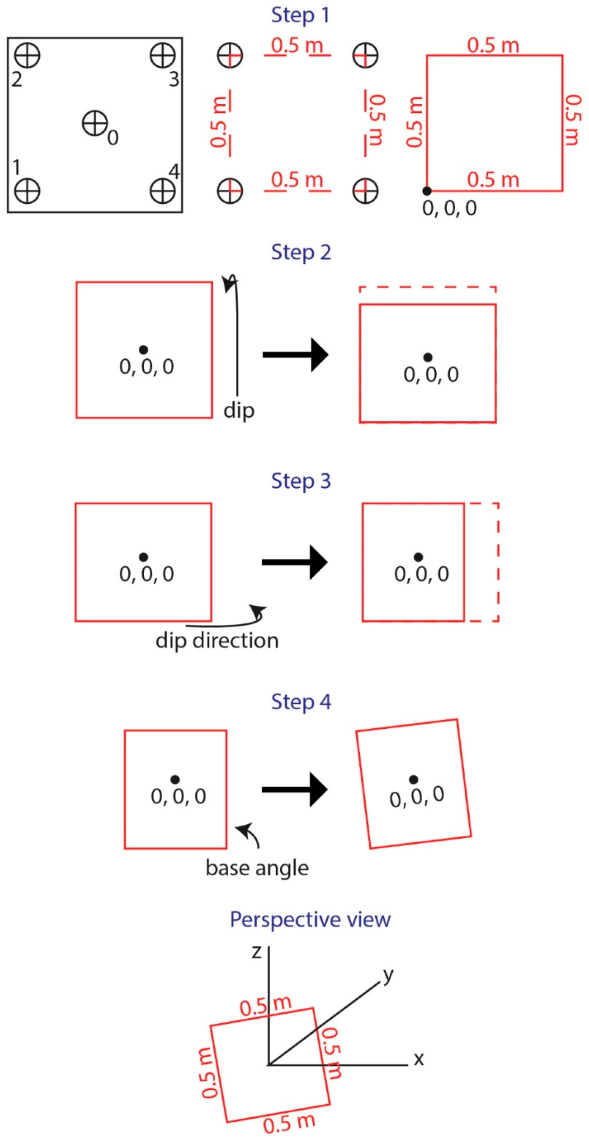
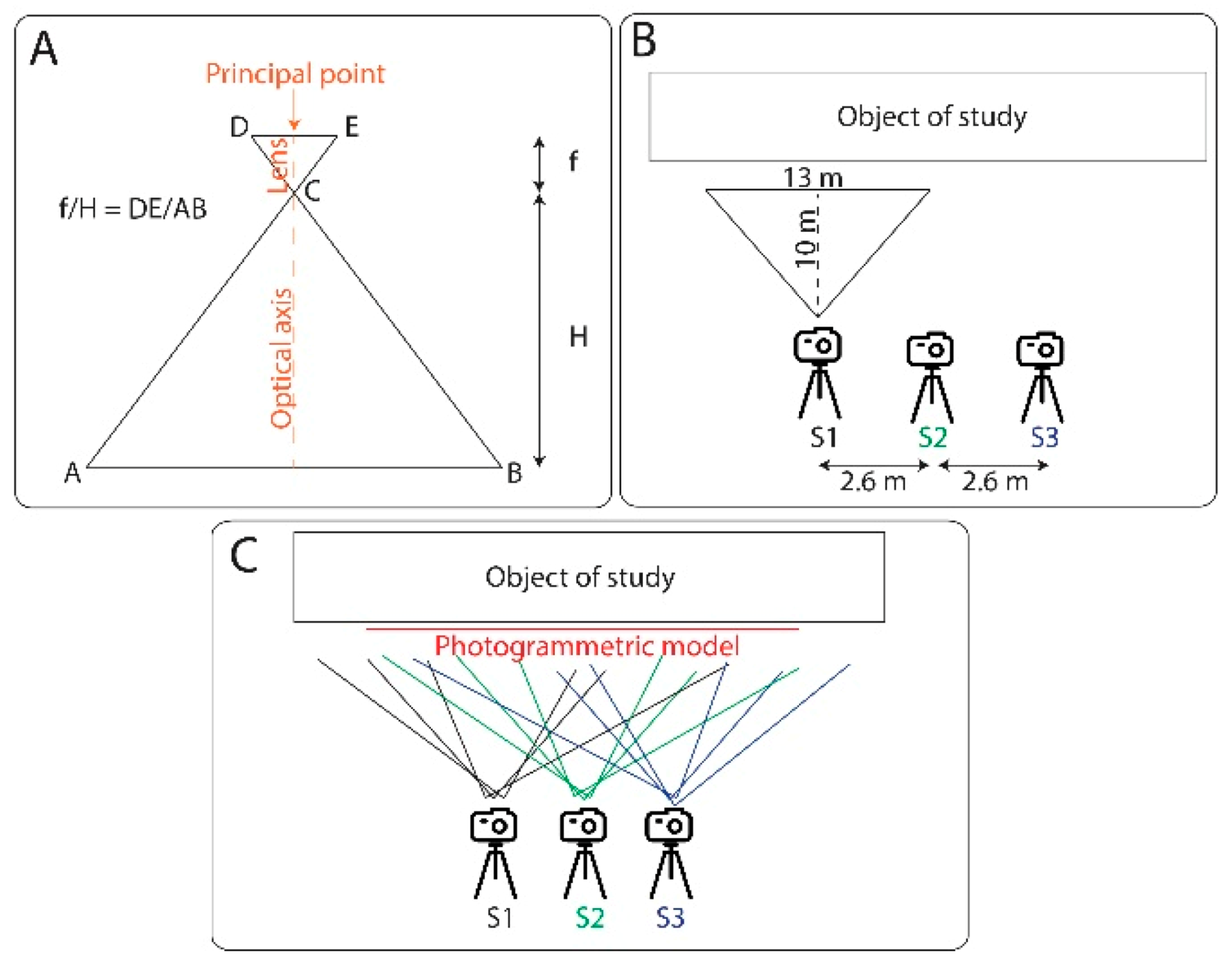
2.1. Defining the Coordinate of the Targets
2.2. DP Surveys
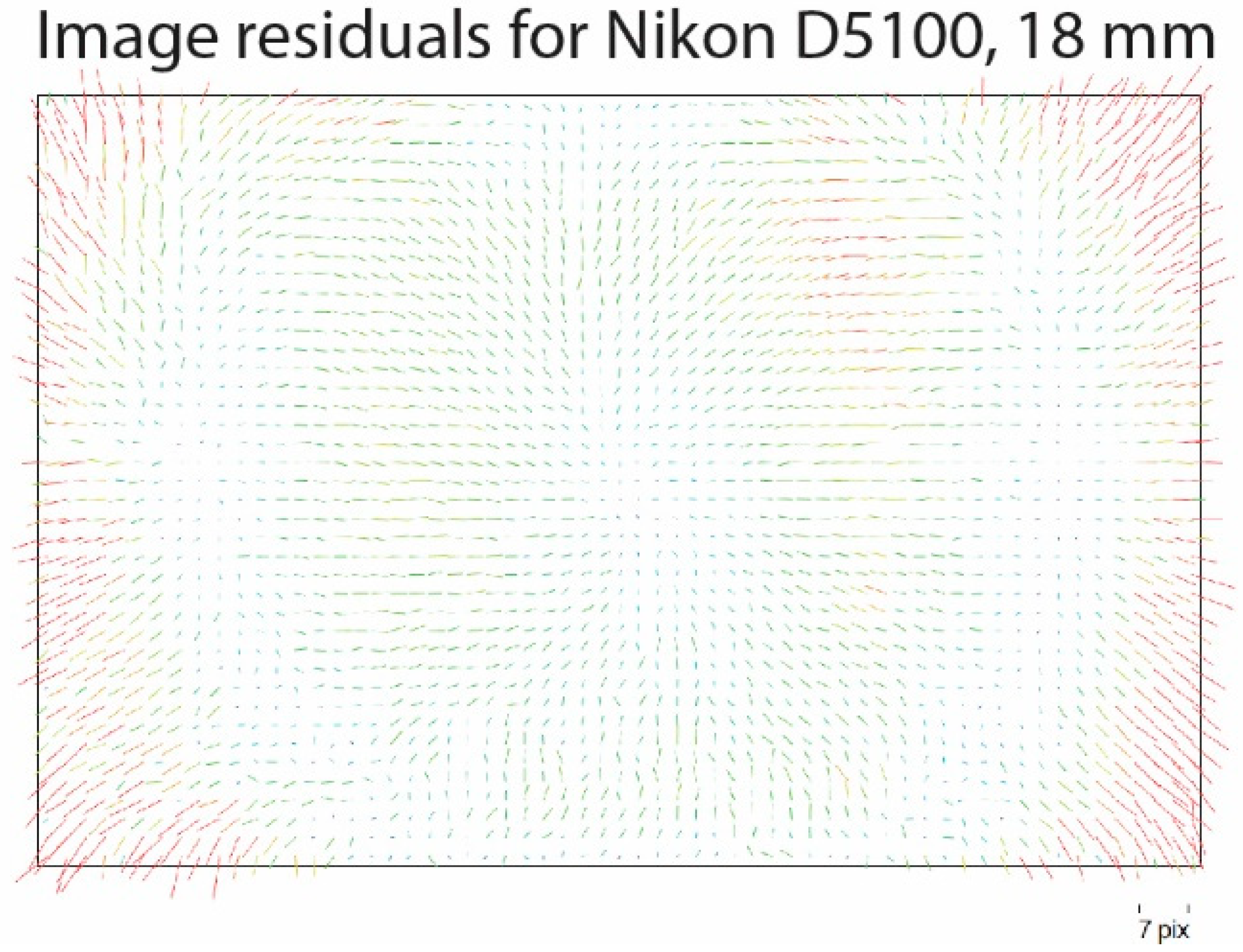
2.2.1. DP Surveys with Calibrated and Non-Calibrated Cameras
- fx, fy = focal length
- cx, cy = principal point coordinates
- K1, K2, K3, P1, P2 = radial distortion coefficients, using Brown’s distortion model
2.2.2. DP Surveys with Smartphones
2.3. LS Surveys
3. Results
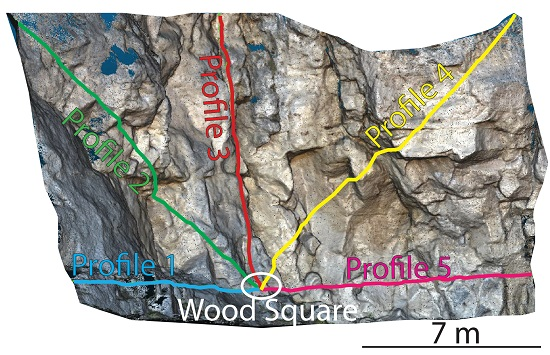
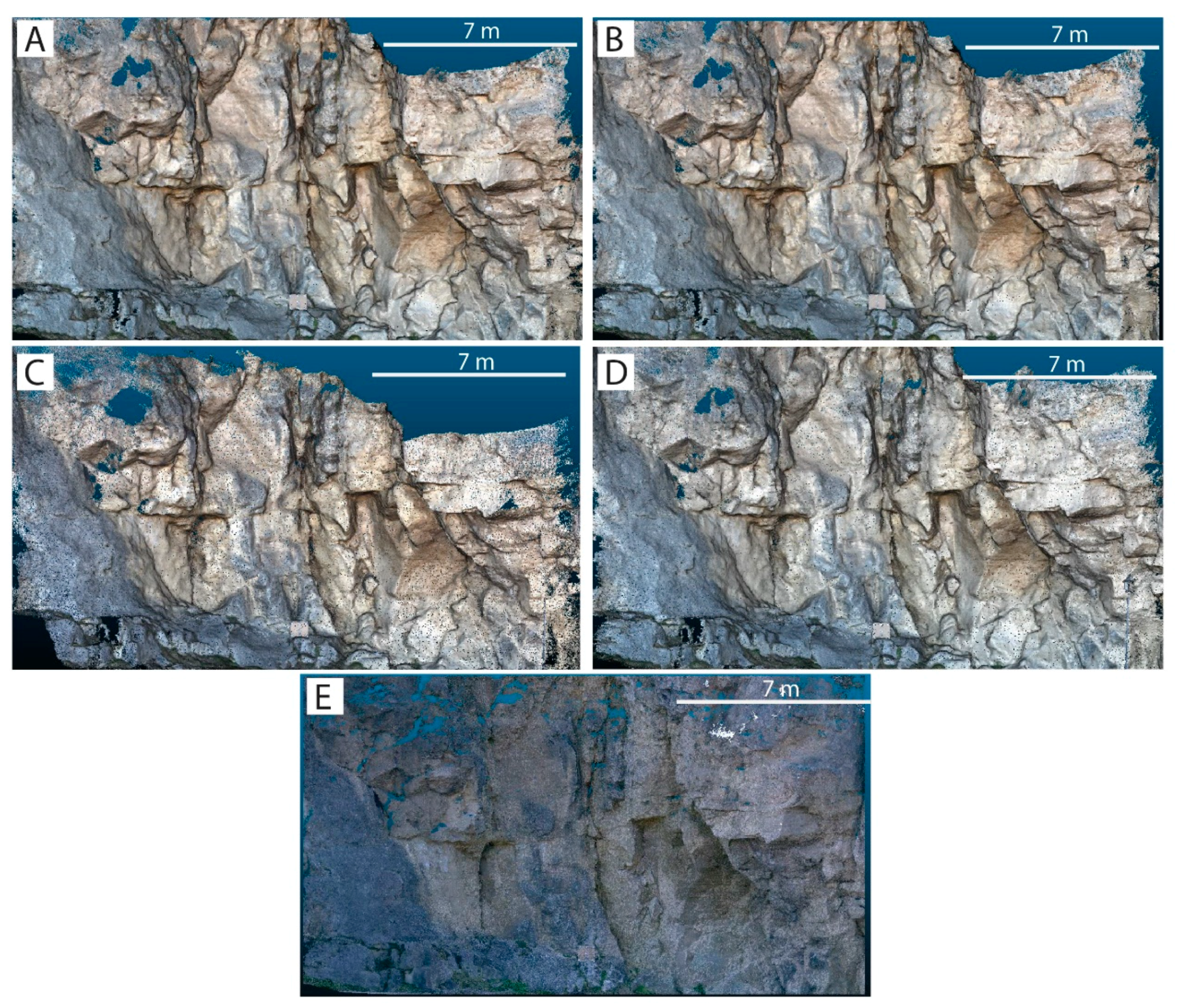
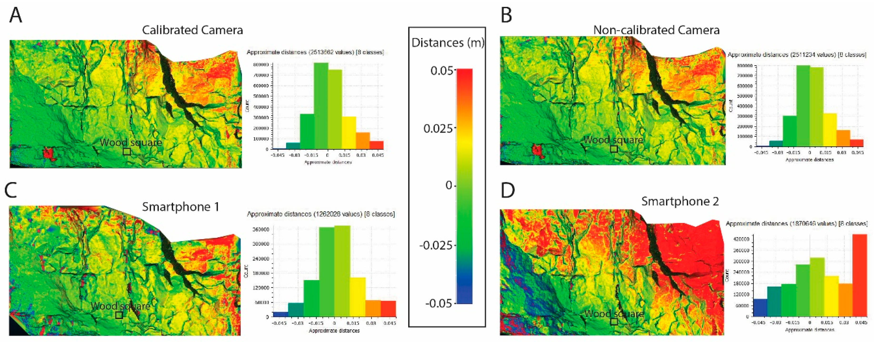
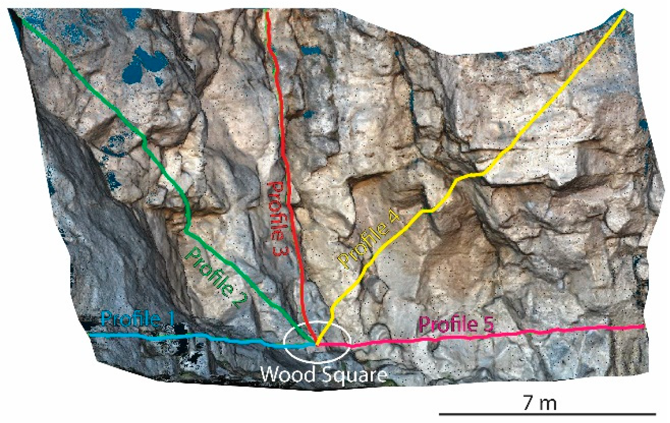
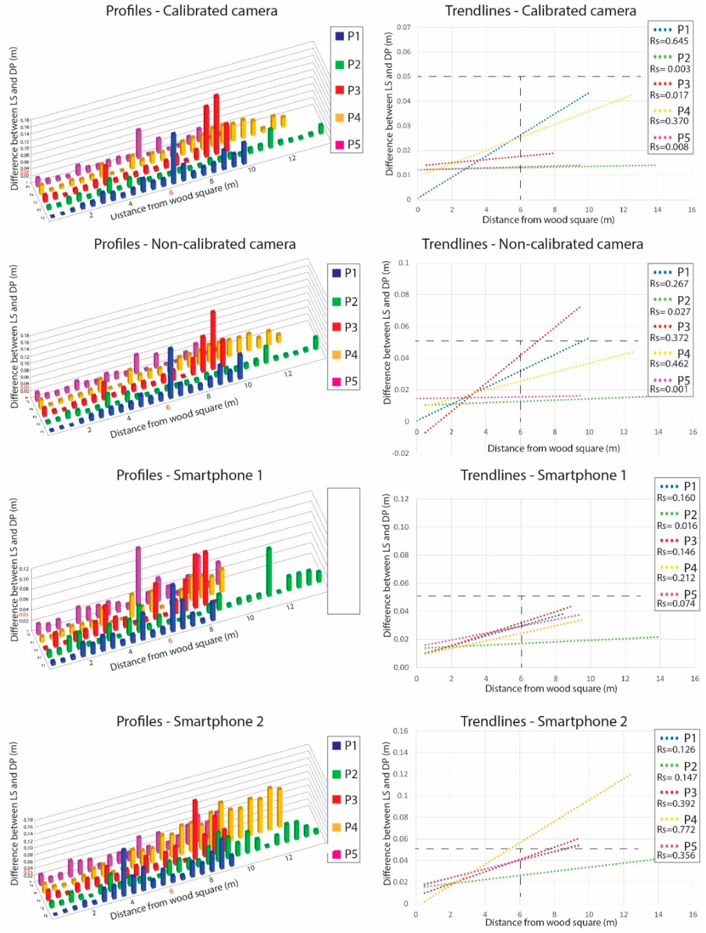
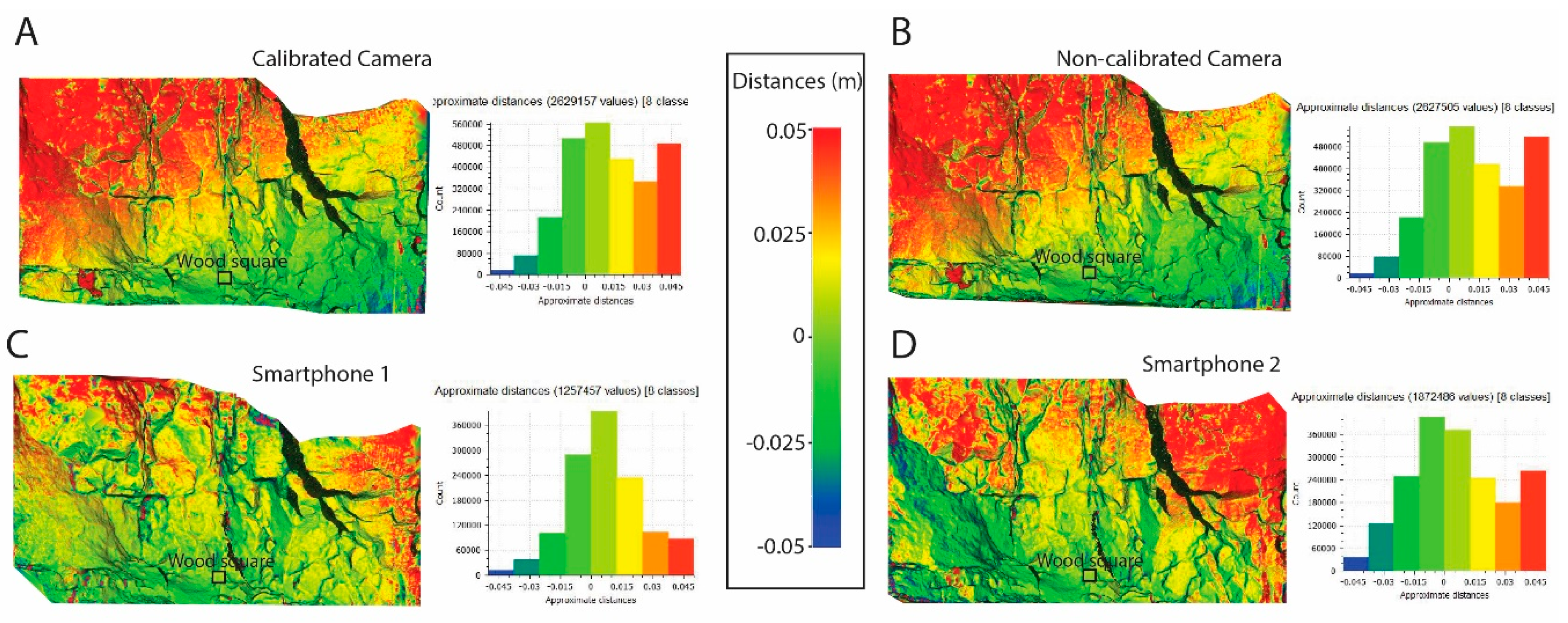
3.1. Analysis of DP and LS Data Using Wooden Square Targets 1, 2, 3, 4 and 5
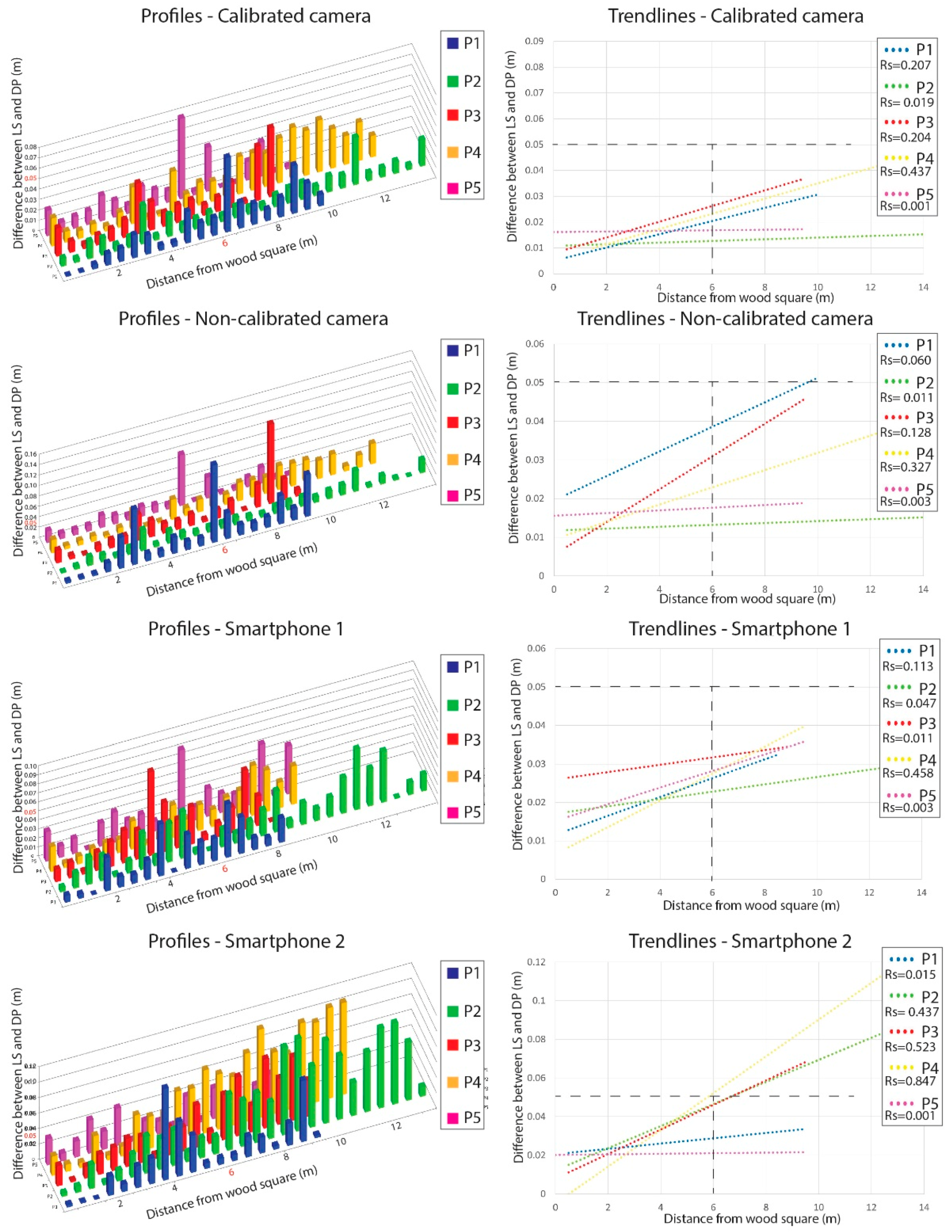
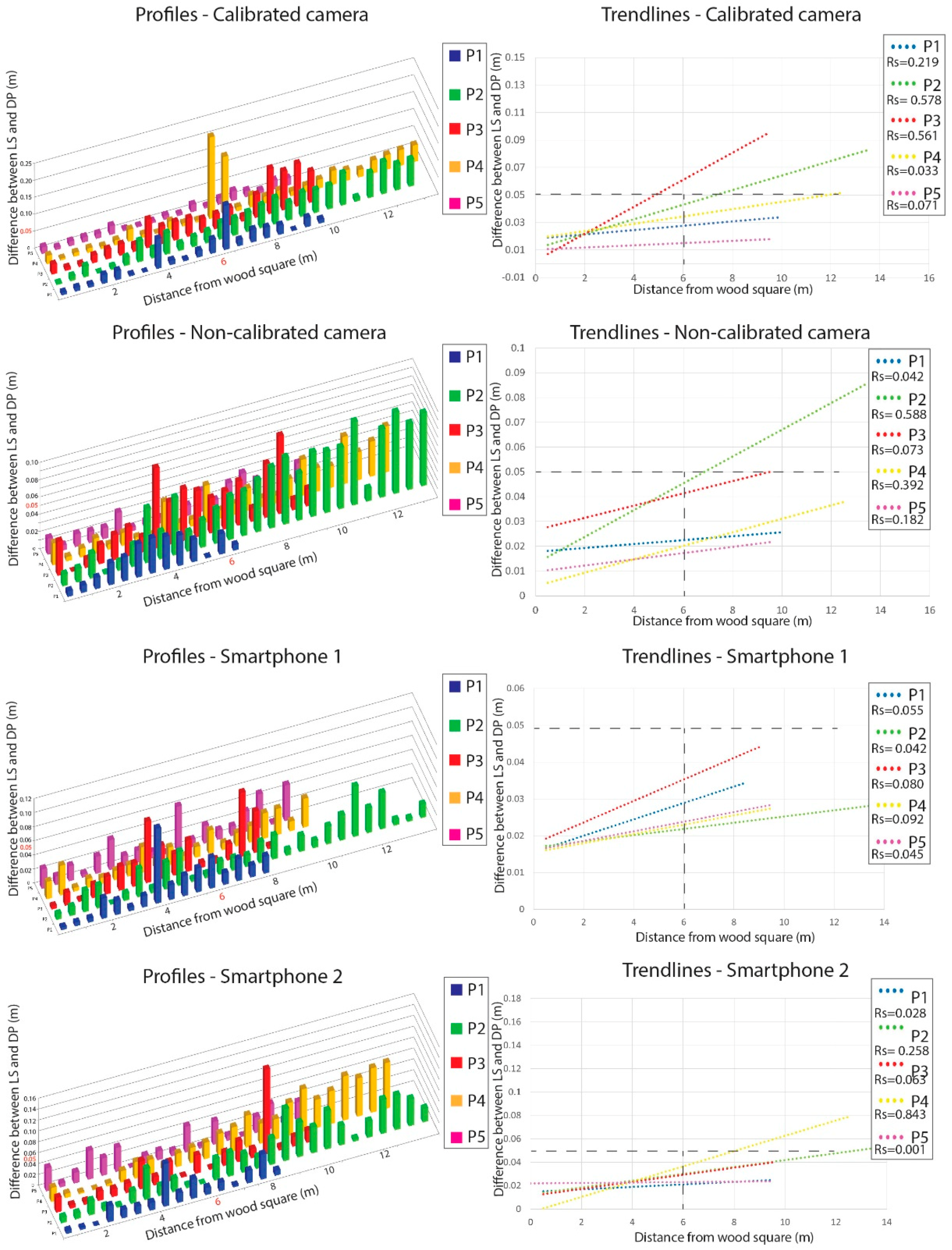
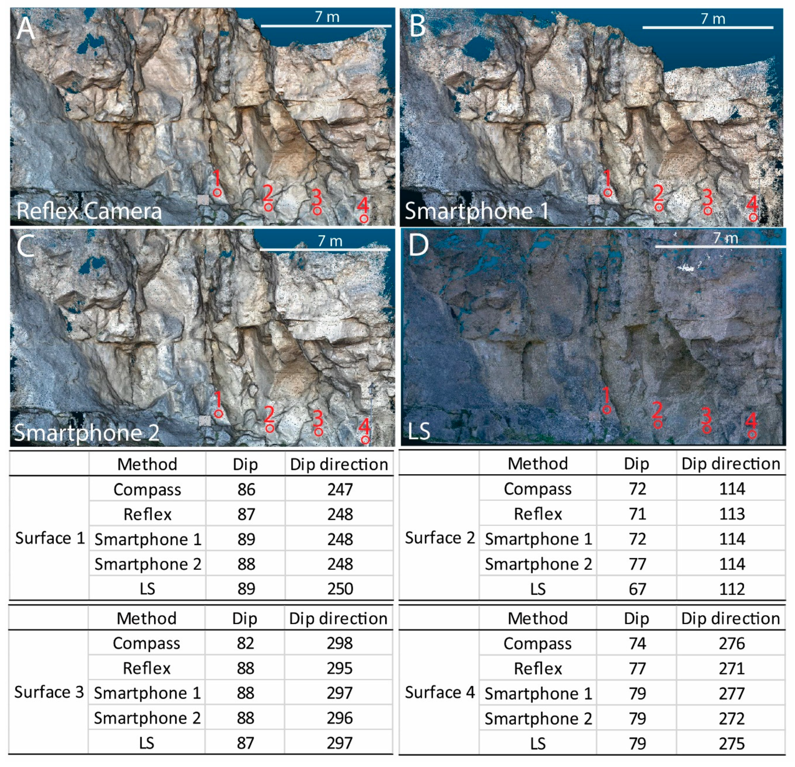
3.2. Analysis of the DP and LS Data Using the Three Targets 1, 2 and 3
3.3. Analysis of the DP and LS Data Using the Three Targets 0, 5, and 3
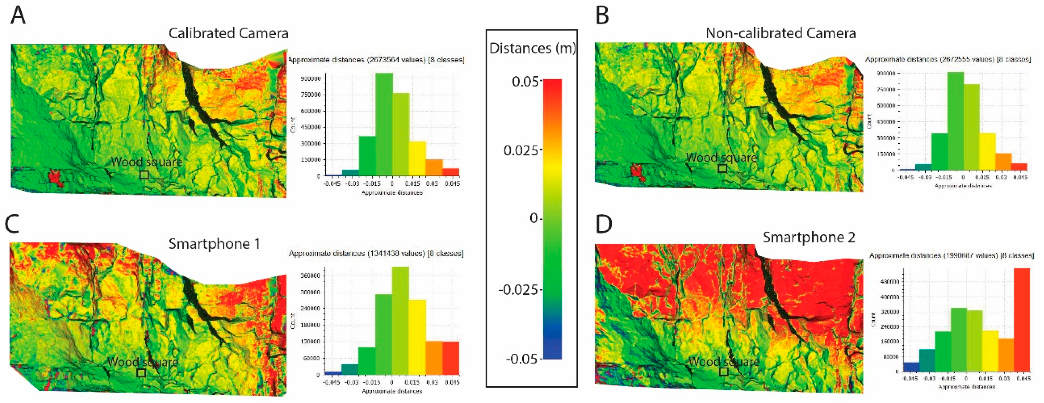
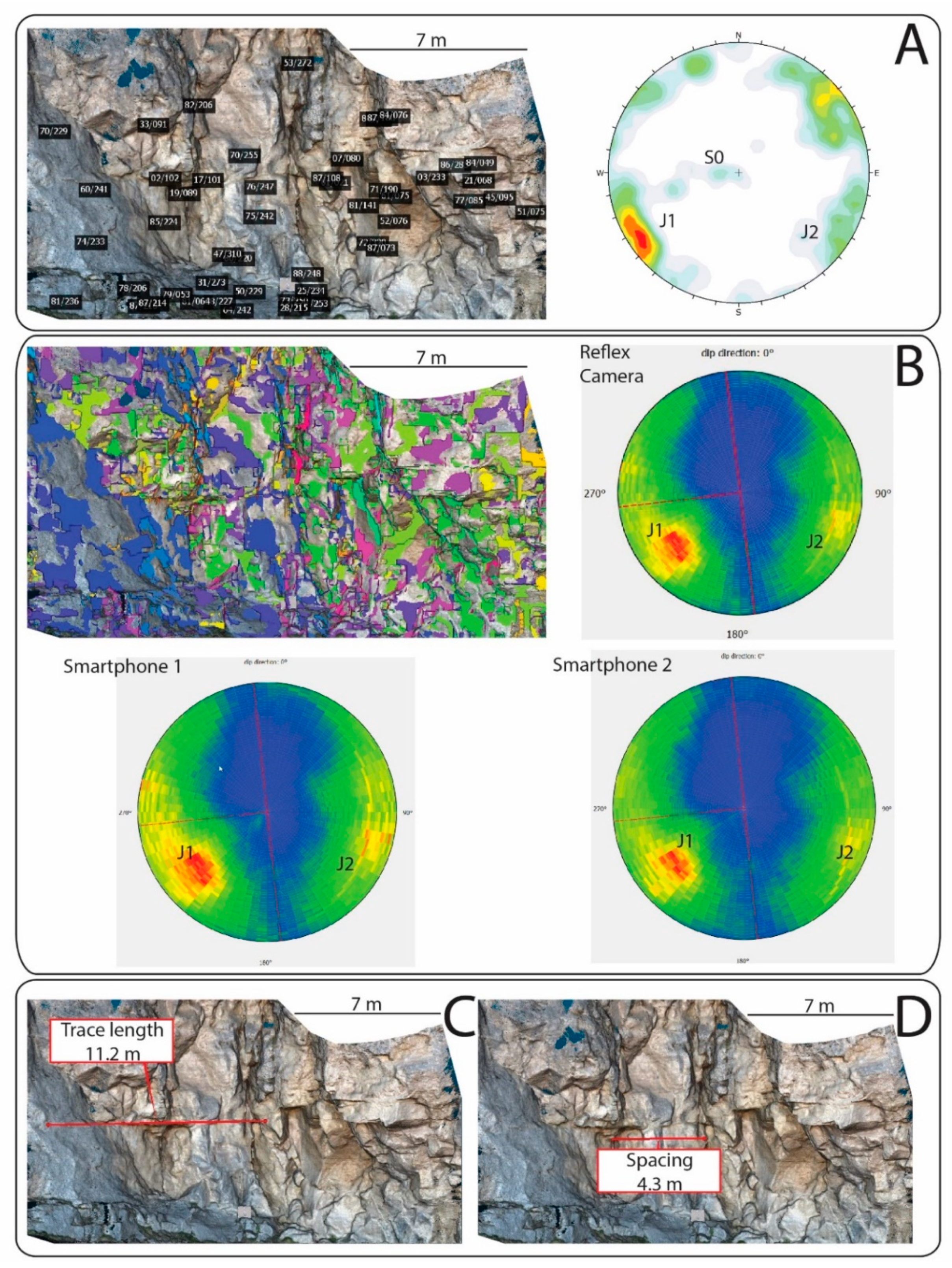
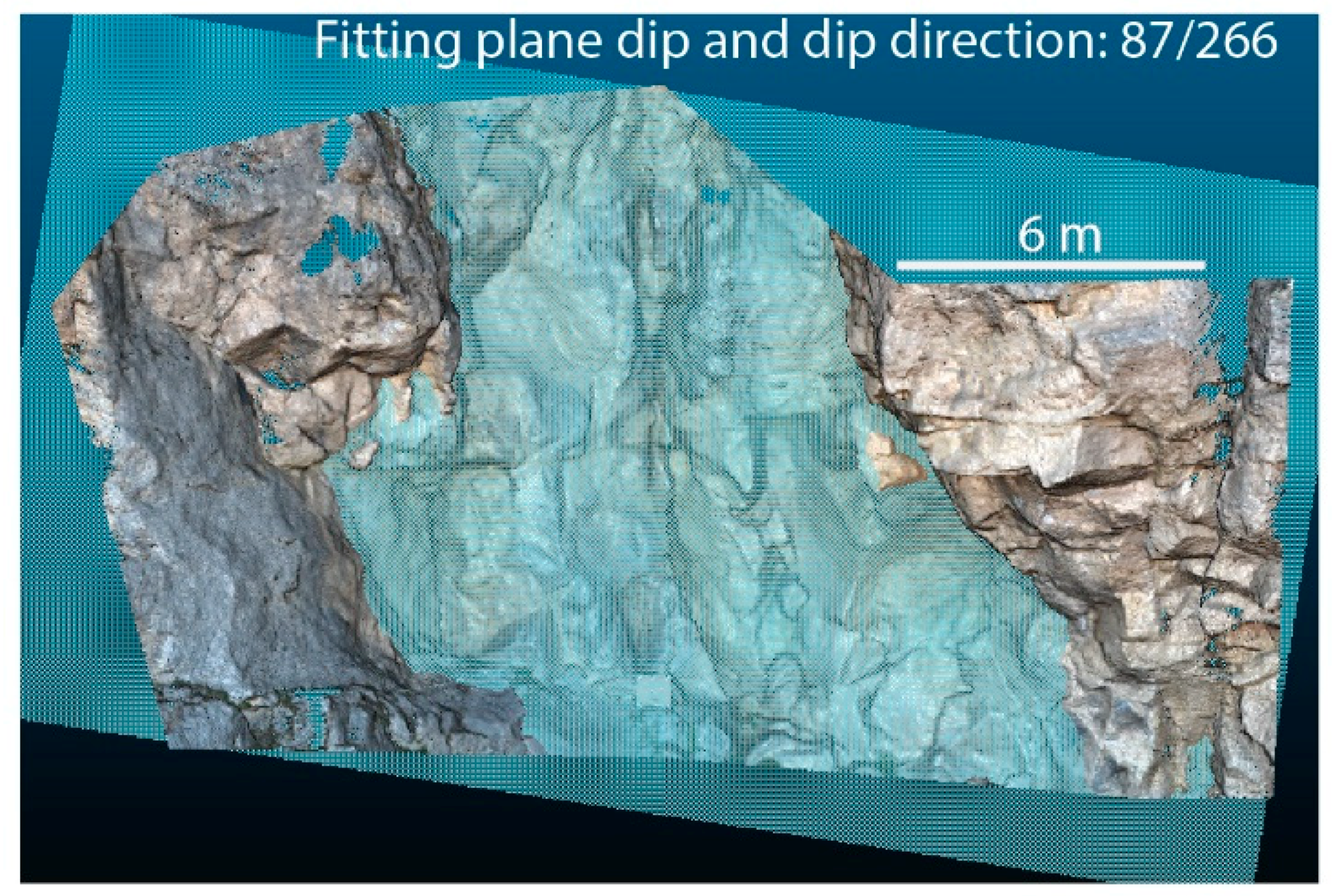
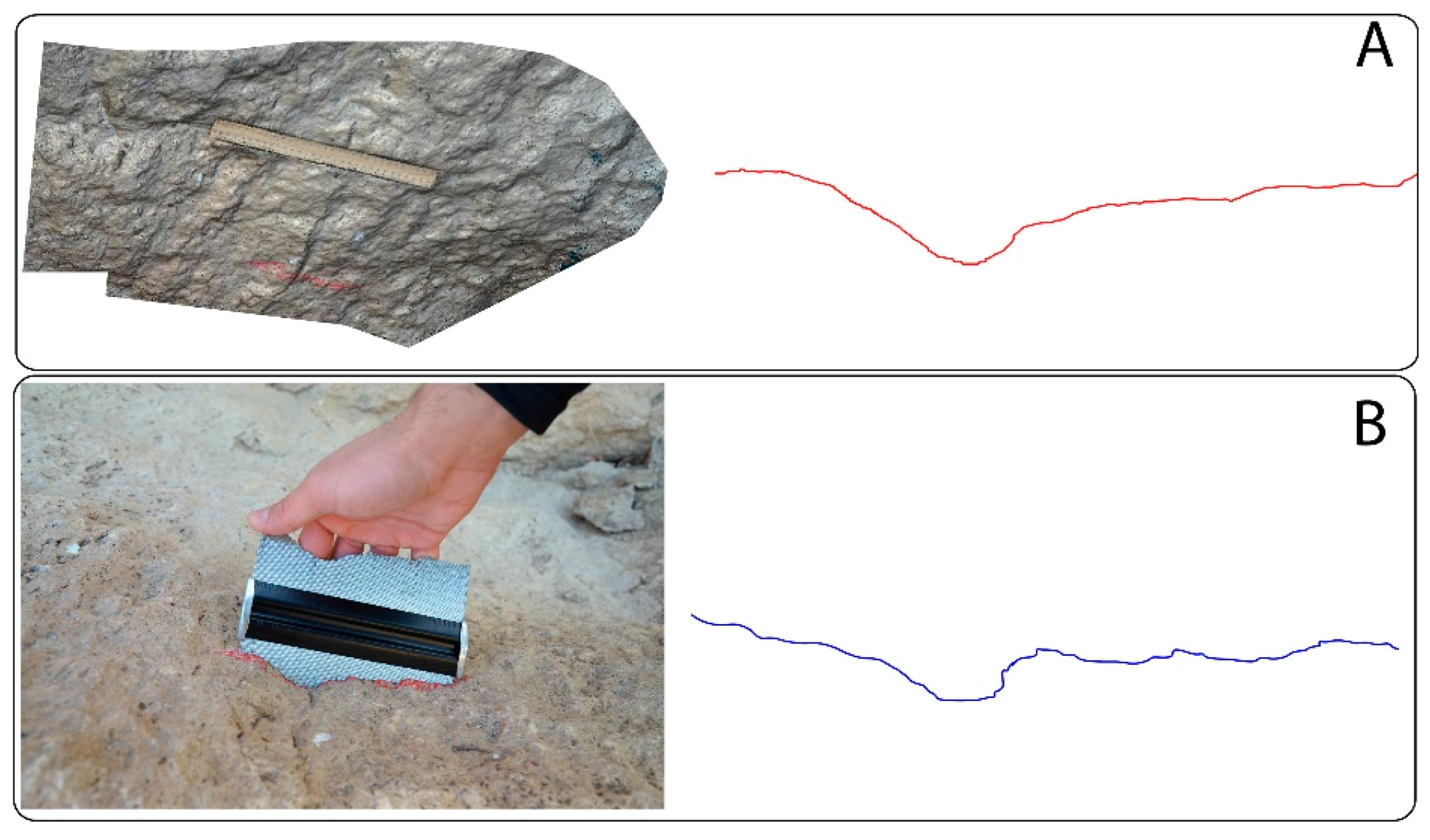
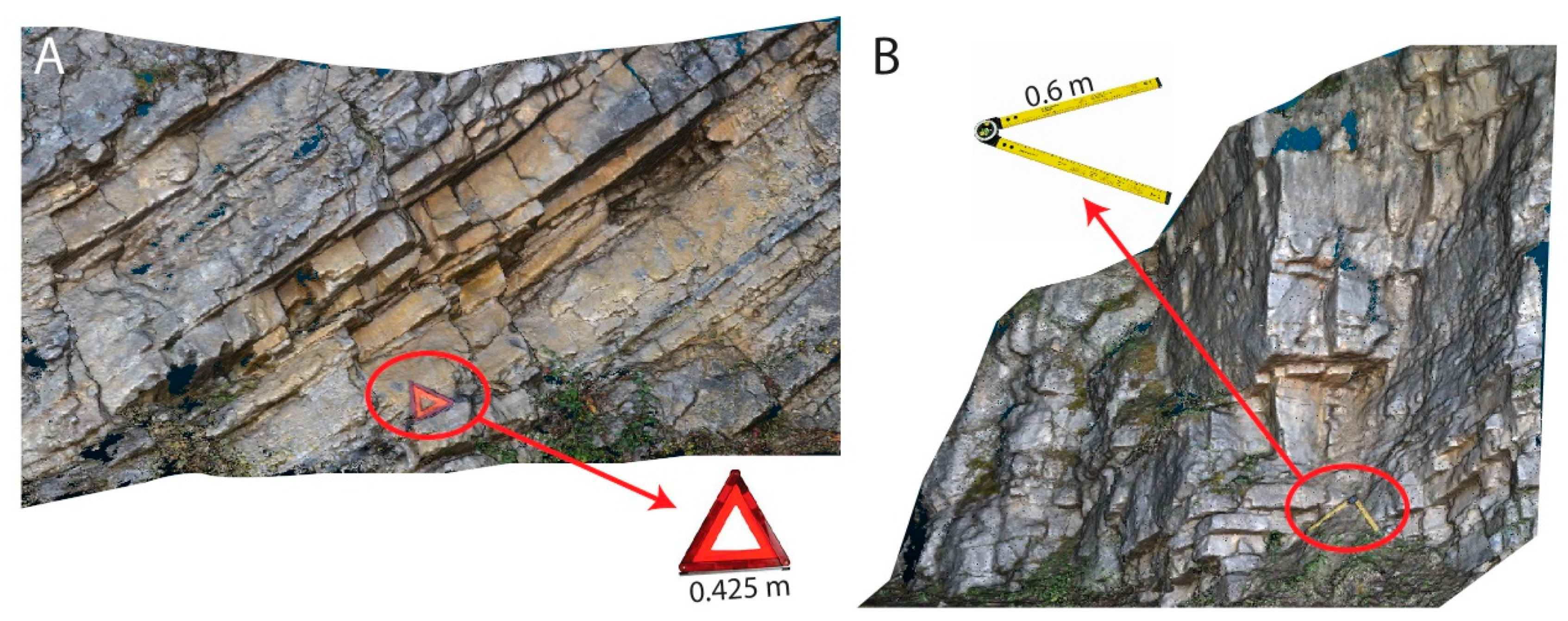
3.4. Potential Engineering Geological Data Derived from DP Models
4. Discussion
5. Conclusions
Author Contributions
Funding
Acknowledgments
Conflicts of Interest
References
- Salvini, R.; Francioni, M.; Riccucci, S.; Bonciani, F.; Callegari, I. Photogrammetry and laser scanning for analyzing slope stability and rock fall runout along the Domodossola? Iselle railway, the Italian Alps. Geomorphology 2013, 185, 110–122. [Google Scholar] [CrossRef]
- Francioni, M.; Salvini, R.; Stead, D.; Giovannini, R.; Riccucci, S.; Vanneschi, C.; Gulli, D. An integrated remote sensing-GIS approach for the analysis of an open pit in the Carrara marble district, Italy: Slope stability assessment through kinematic and numerical methods. Comput. Geotech. 2015, 67, 46–63. [Google Scholar] [CrossRef]
- Spreafico, M.C.; Cervi, F.; Francioni, M.; Stead, D.; Borgatti, L. An investigation into the development of toppling at the edge of fractured rock plateaux using a numerical modelling approach. Geomorphology 2017, 288, 83–98. [Google Scholar] [CrossRef]
- Wolter, A.; Stead, D.; Ward, B.C.; Clague, J.J.; Ghirotti, M. Engineering geomorphological characterisation of the Vajont Slide, Italy, and a new interpretation of the chronology and evolution of the landslide. Landslides 2016, 5, 1067–1081. [Google Scholar] [CrossRef]
- Donati, D.; Stead, D.; Ghirotti, M.; Brideau, M.-A. A model-oriented, remote sensing approach for the derivation of numerical modelling input data: Insights from the Hope Slide, Canada. In Proceedings of the ISRM International Symposium ‘Rock Mechanics for Africa’ AfriRock Conference, Cape Town, South Africa, 3–5 October 2017. [Google Scholar]
- Mazzanti, P.; Schilirò, L.; Martino, S.; Antonielli, B.; Brizi, E.; Brunetti, A.; Margottini, C.; Mugnozza, G.S. The contribution of terrestrial laser scanning to the analysis of cliff slope stability in Sugano (Central Italy). Remote Sens. 2018, 10, 1475. [Google Scholar] [CrossRef]
- Birch, J.S. Using 3DM Analyst mine mapping suite for rock face characterization. In Laser and Photogrammetric Methods for Rock Face Characterization; Tonon, F., Kottenstette, J., Eds.; ARMA: Golden, CO, USA, 2006; pp. 13–32. [Google Scholar]
- Francioni, M.; Salvini, R.; Stead, D.; Coggan, J.J. Improvements in the integration of remote sensing and rock slope modelling. Nat. Hazards 2018, 90, 975–1004. [Google Scholar] [CrossRef]
- Sturzenegger, M.; Stead, D. Close-range terrestrial digital photogrammetry and terrestrial laser scanning for discontinuity characterization on rock cuts. Eng. Geol. 2009, 106, 163–182. [Google Scholar] [CrossRef]
- Westoby, M.J.; Brasington, J.; Glasser, N.F.; Hambrey, M.J.; Reynolds, J.M. ‘Structure-from-Motion’ photogrammetry: A low-cost, effective tool for geoscience applications. Geomorphology 2012, 179, 300–314. [Google Scholar] [CrossRef]
- Salvini, R.; Riccucci, S.; Gullì, D.; Giovannini, R.; Vanneschi, C.; Francioni, M. Geological application of UAV photogrammetry and terrestrial laser scanning in marble quarrying (Apuan Alps, Italy). Eng. Geol. Soc. Territ. 2015, 5, 979–983. [Google Scholar]
- Francioni, M.; Coggan, J.; Eyre, M.; Stead, D. A combined field/remote sensing approach for characterizing landslide risk in coastal areas. Int. J. Appl. Earth Obs. Geoinf. 2018, 67, 79–95. [Google Scholar] [CrossRef]
- Francioni, M.; Stead, D.; Sciarra, N.; Calamita, F. A new approach for defining Slope Mass Rating in heterogeneous sedimentary rocks using a combined remote sensing GIS approach. Bull. Eng. Geol. Environ. 2019, in press. [Google Scholar] [CrossRef]
- Agisoft. Agisoft Photoscan (version 1.4) 2018. Available online: http://www.agisoft.com/ (accessed on 2 July 2018).
- Leica-geosystems. 2019. Available online: https://leica-geosystems.com/products/laser-scanners/scanners/blk360 (accessed on 7 January 2019).
- CloudCompare V.2.9, GPL Software 2018. Available online: http://www.cloudcompare.org/ (accessed on 2 July 2018).
- Dewez, T.J.B.; Girardeau-Montaut, D.; Allanic, C.; Rohmer, J. Facets: A Cloudcompare Plugin to Extract Geological Planes from Unstructured 3D Point Clouds. ISPRS Int. Arch. Photogramm. Sens. Spat. Inf. Sci. 2016, XLI-B5, 799–804. [Google Scholar] [CrossRef]
- Dershowitz, W.S.; Herda, H.H. Interpretation of fracture spacing and intensity. In Proceedings of the 33rd US Symposium on Rock Mechanics, Santa Fe, NM, USA, 3–5 June 1992; pp. 757–766. [Google Scholar]
- Francioni, M.; Salvini, R.; Stead, D.; Litrico, S. A case study integrating remote sensing and distinct element analysis to quarry slope stability assessment in the Monte Altissimo area, Italy. Eng. Geol. 2014, 183, 290–302. [Google Scholar] [CrossRef]
- Oniga, V.-E.; Breaban, A.-I.; Stătescu, F. Determining the Optimum Number of Ground Control Points for Obtaining High Precision Results Based on UAS Images. Proceedings 2018, 2, 352. [Google Scholar] [CrossRef]
- Novakova, L.; Pavlis, T.L. Assessment of the precision of smart phones and tablets for measurement of planar orientations: A case study. J. Struct. Geol. 2017, 97, 93–103. [Google Scholar] [CrossRef]
- Haneberg, W.C. Directional roughness profiles from three-dimensional photogrammetric or laser scanner point clouds. In Proceedings of the 1st Canada-U.S. Rock Mechanics Symposium, Vancouver, BC, Canada, 27–31 May 2007; pp. 101–106. [Google Scholar]
- Poropat, G. Remote characterisation of surface roughness of rock discontinuities. In 1st Southern Hemisphere International Rock Mechanics Symposium; Australian Centre for Geomechanics: Perth, Australia, 2008. [Google Scholar]
- Kim, D.H.; Gratchev, I.; Balasubramaniam, A. Determination of joint roughness coefficient (JRC) for slope stability analysis: A case study from the Gold Coast area, Australia. Landslides 2013, 10, 657–664. [Google Scholar] [CrossRef]
- Tong, X.; Liu, X.; Chen, P.; Liu, S.; Luan, K.; Li, L.; Liu, S.; Liu, X.; Xie, H.; Jin, Y.; et al. Integration of UAV-Based Photogrammetry and Terrestrial Laser Scanning for the Three-Dimensional Mapping and Monitoring of Open-Pit Mine Areas. Remote Sens. 2015, 7, 6635–6662. [Google Scholar] [CrossRef]
- Caporossi, P.; Mazzanti, P.; Bozzano, F. Digital Image Correlation (DIC) Analysis of the 3 December 2013 Montescaglioso Landslide (Basilicata, Southern Italy): Results from a Multi-Dataset Investigation. ISPRS Int. J. GeoInf. 2018, 7, 372. [Google Scholar] [CrossRef]
- Wu, C. VisualSFM: A Visual Structure from Motion System. 2011. Available online: http://www.cs.washington.edu/homes/ccwu/vsfm/ (accessed on 2 July 2018).


| Parameter | Value (pixel) | Standard Error |
|---|---|---|
| Image width | 4928 | |
| Image height | 3264 | |
| Principal point (x) | 19.9889 | 0.890748 |
| Principal point (y) | 36.4507 | 0.89439 |
| Radial K1 | −0.0628401 | 0.00235961 |
| Radial K2 | 0.0652221 | 0.0132876 |
| Radial K3 | −0.105281 | 0.0295335 |
| Radial K4 | 0.0729408 | 0.000503861 |
| Tangential P1 | −0.000123014 | 5.1837e-05 |
| Tangential P2 | 0.000487723 | 3.7193e-05 |
| ID | X (m) | Y (m) | Z (m) |
|---|---|---|---|
| 0 | 0 | 0 | 0 |
| 1 | −0.081 | 0.25 | −0.236 |
| 2 | 0.081 | 0.25 | 0.236 |
| 3 | 0.081 | −0.25 | 0.236 |
| 4 | −0.081 | −0.25 | −0.236 |
| 5 | 0.081 | 0 | 0.236 |
| Type of Survey | Model Resolution (m) |
|---|---|
| LS | 0.003–0.010 |
| DP calibrated camera | 0.010 |
| DP non-calibrated camera | 0.010 |
| Smartphone 1 | 0.015 |
| Smartphone 2 | 0.012 |
| DP Technique | Advantages | Limitation |
|---|---|---|
| DP with hand-held reflex camera and TS or GPS | Full control of the camera. Photographs can be acquired with great precision without problems associated with lateral extent of the outcrop. Total stationallows to acquire GCPs on the entire outcrop surface. The DP model created using TS GCP will be very accurate. Data extracted can be used for engineering geological interpretation and data extraction. | Cost of the instrumentation includes both the digital camera and TS/GPS. Presence of occlusions in the case of very high slopes. Difficult/impossible to use in poorly accessible areas. |
| DP with hand-held reflex camera and object of known geometry | Full control of the camera. Photographs can be acquired with great precision. High portability of the instrumentation. Limits the cost incurred to the use of a digital camera. Reduces the time of the survey and therefore decreases the risk to the surveyor. Data extracted can be used for engineering geological interpretation and post processing. | Cost of the instrumentation limited to the digital camera. Presence of occlusions in the case of very high slopes. The precision of the DP models is more influenced by the object used for georeferencing and decreases toward the outer limits of the derived models. |
| DP with smartphones and object of known geometry | Precision of photographs is limited according to the smartphone used. Very high portability of the instrumentation and cost-free. Reduces the time of the survey and therefore decreases the risk to the surveyor. Data extracted can be used for engineering geological interpretation and post processing. | Presence of occlusions in the case of very high slopes. The precision of the DP models is more highly influenced by the object used for georeferencing and decreases toward the outer extent of the derived models. The precision is also strongly influenced by the type of smartphone camera used. Therefore, when using the smartphone to obtain DP it is highly recommended to always validate the data against field measurements. |
© 2019 by the authors. Licensee MDPI, Basel, Switzerland. This article is an open access article distributed under the terms and conditions of the Creative Commons Attribution (CC BY) license (http://creativecommons.org/licenses/by/4.0/).
Share and Cite
Francioni, M.; Simone, M.; Stead, D.; Sciarra, N.; Mataloni, G.; Calamita, F. A New Fast and Low-Cost Photogrammetry Method for the Engineering Characterization of Rock Slopes. Remote Sens. 2019, 11, 1267. https://doi.org/10.3390/rs11111267
Francioni M, Simone M, Stead D, Sciarra N, Mataloni G, Calamita F. A New Fast and Low-Cost Photogrammetry Method for the Engineering Characterization of Rock Slopes. Remote Sensing. 2019; 11(11):1267. https://doi.org/10.3390/rs11111267
Chicago/Turabian StyleFrancioni, Mirko, Matteo Simone, Doug Stead, Nicola Sciarra, Giovanni Mataloni, and Fernando Calamita. 2019. "A New Fast and Low-Cost Photogrammetry Method for the Engineering Characterization of Rock Slopes" Remote Sensing 11, no. 11: 1267. https://doi.org/10.3390/rs11111267
APA StyleFrancioni, M., Simone, M., Stead, D., Sciarra, N., Mataloni, G., & Calamita, F. (2019). A New Fast and Low-Cost Photogrammetry Method for the Engineering Characterization of Rock Slopes. Remote Sensing, 11(11), 1267. https://doi.org/10.3390/rs11111267