On the Synergistic Use of Optical and SAR Time-Series Satellite Data for Small Mammal Disease Host Mapping


Abstract
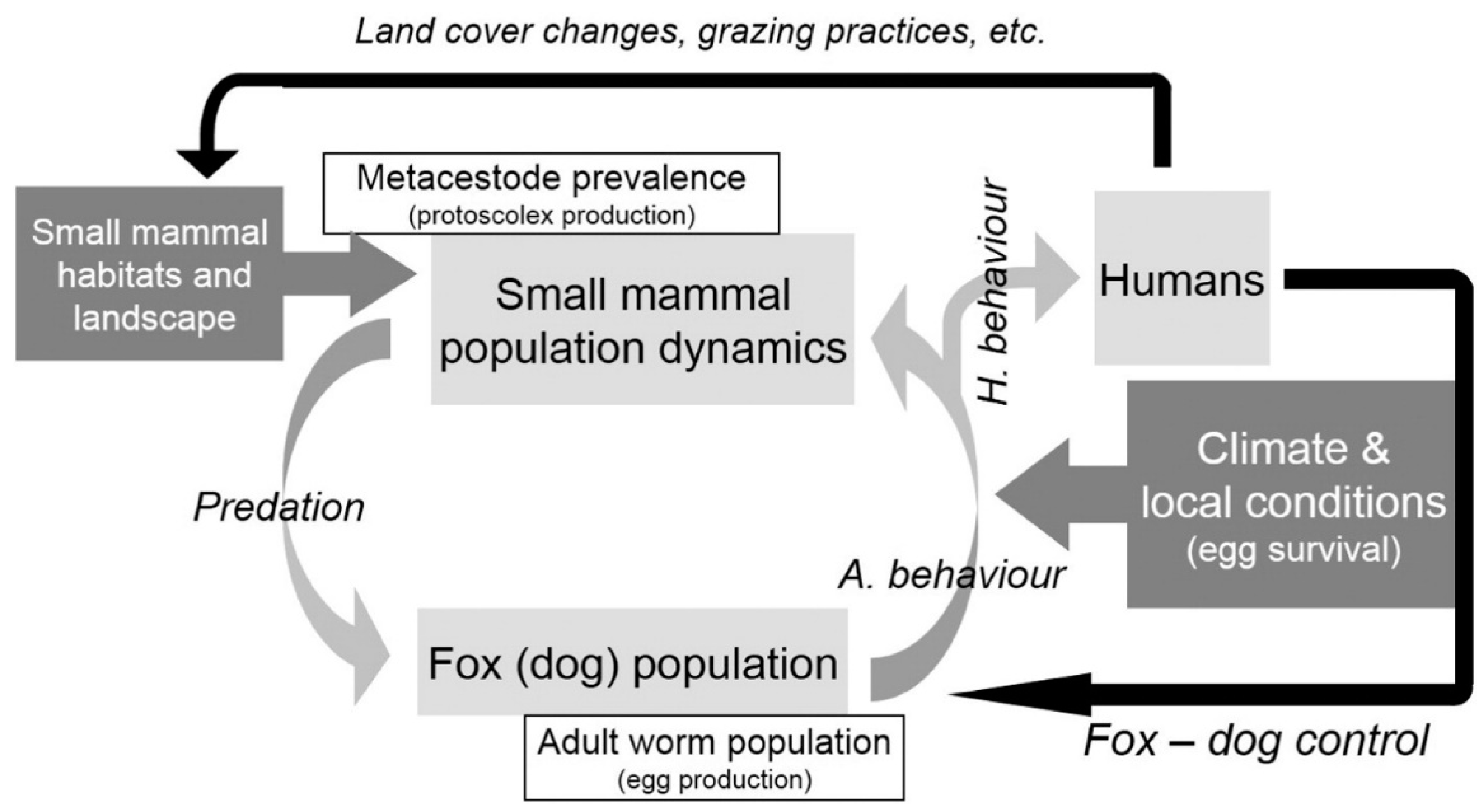
1. Introduction
- (1)
- Can time-series SAR data generate land cover maps of equivalent quality as optical imagery?
- (2)
- What are the key land cover drivers impacting Em host Ellobius tancrei and Microtus gregalis distributions in the study area?
2. Materials and Methods
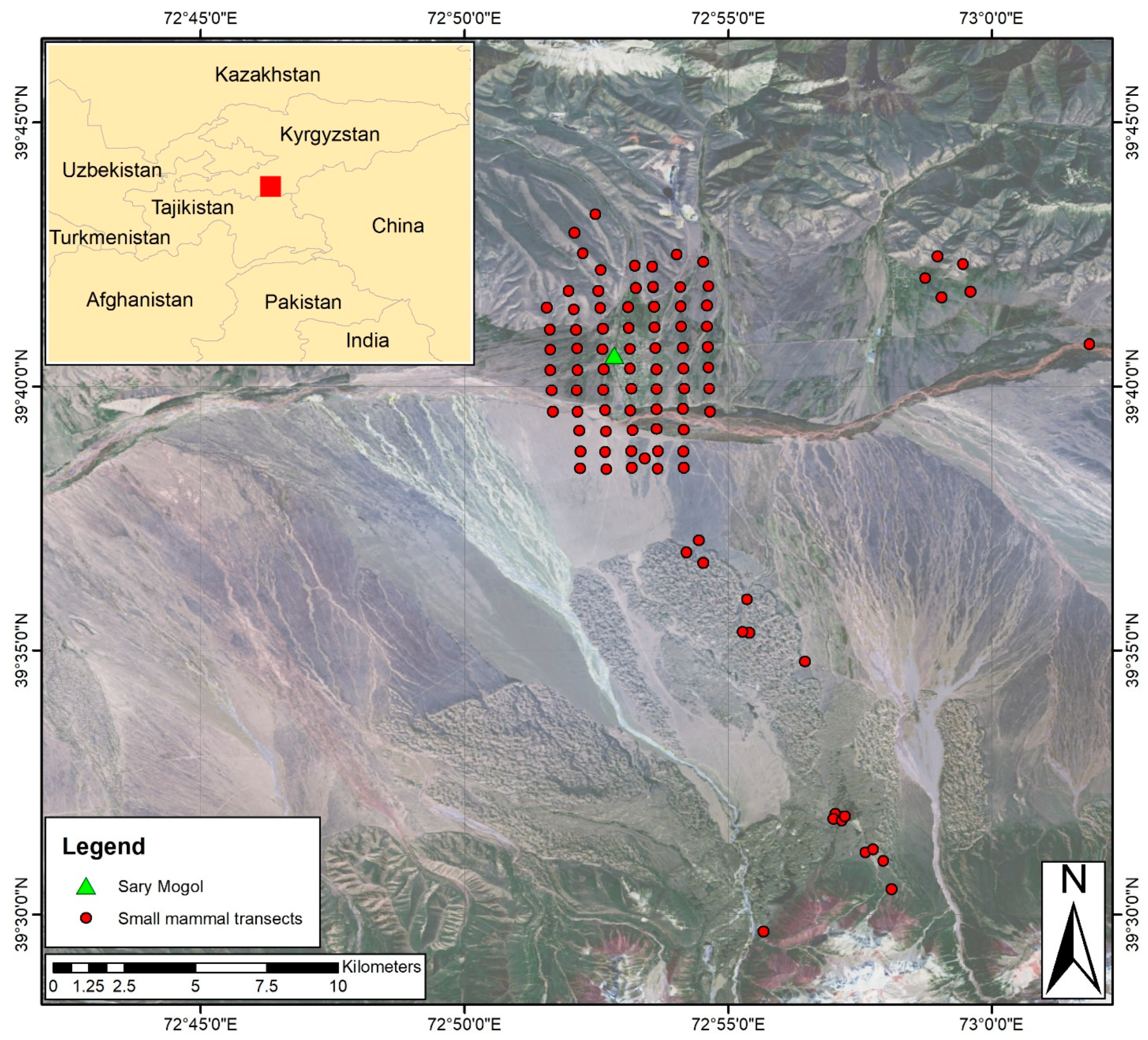
2.1. Study Site
2.2. Satellite Data
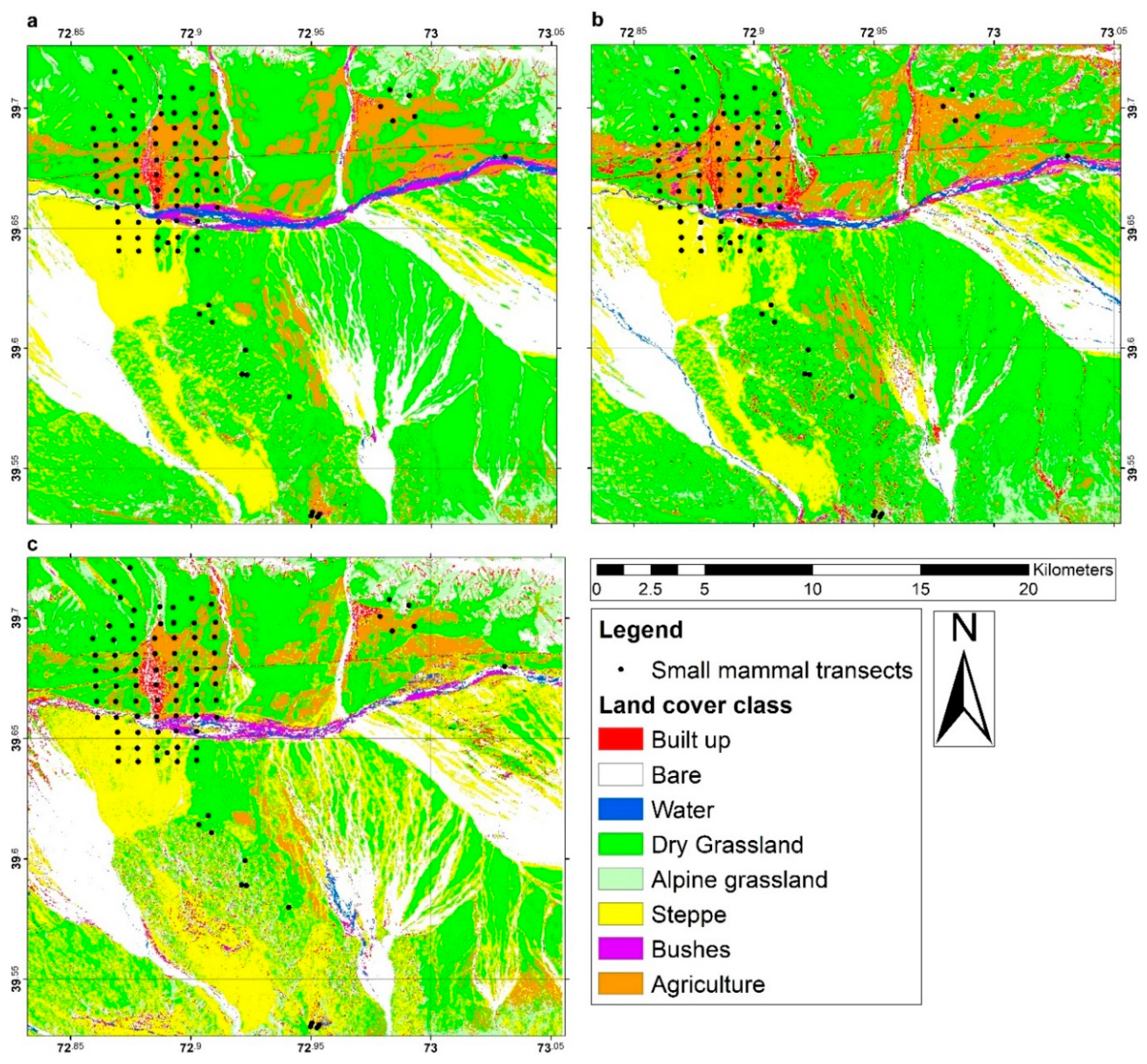
2.3. Land Cover Classification
2.4. Land Cover Data Extraction
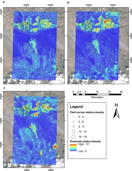
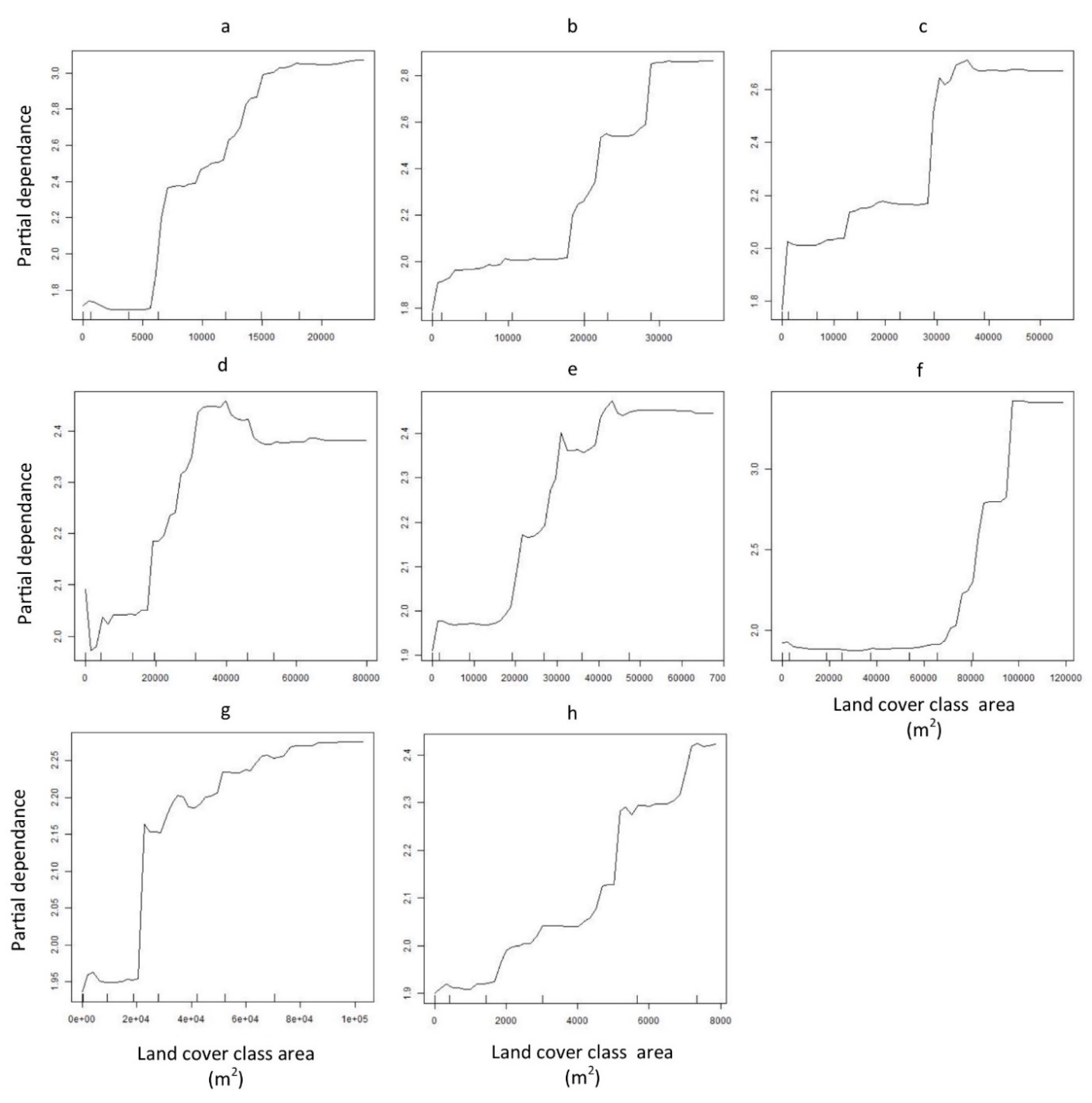
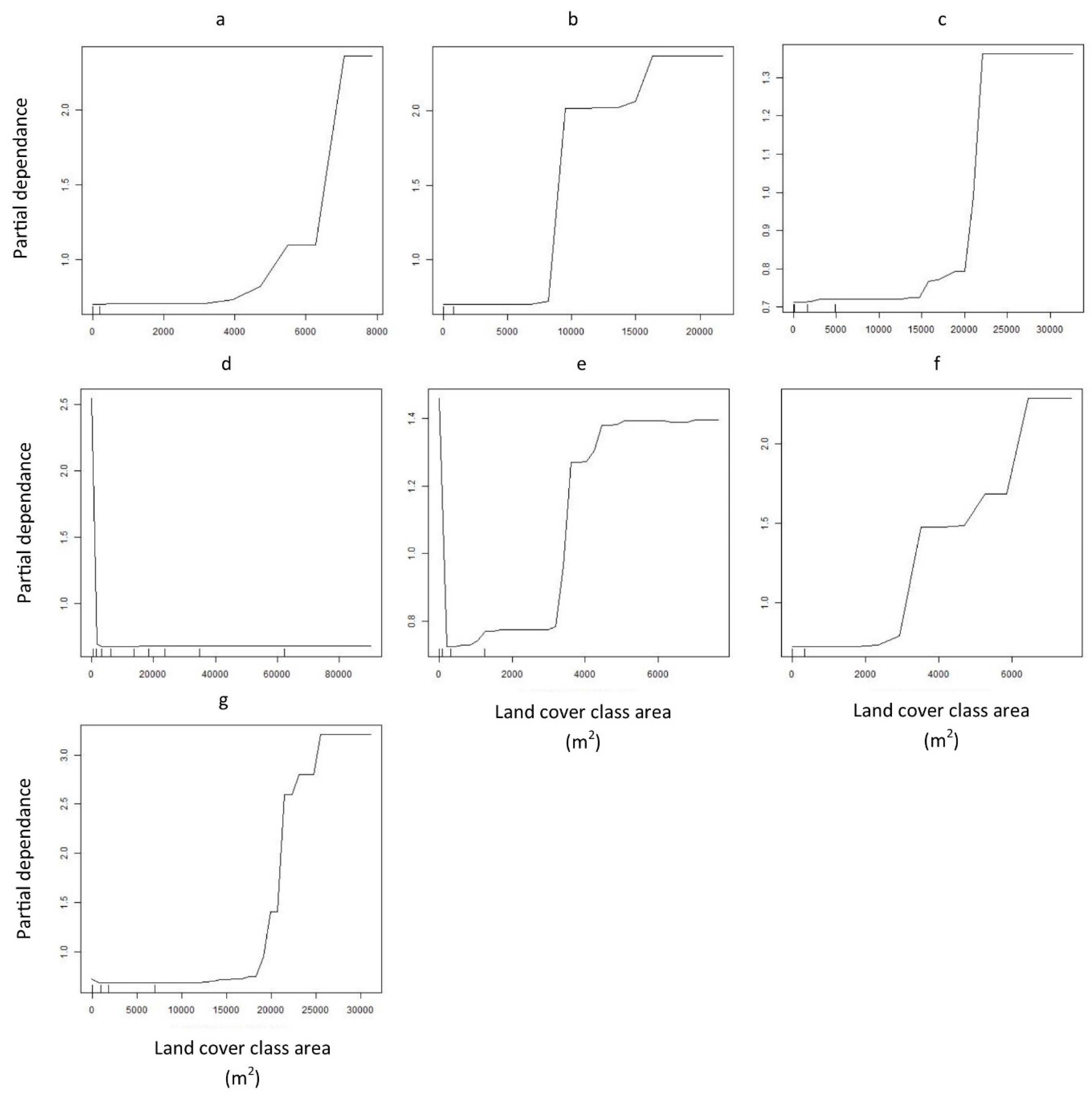
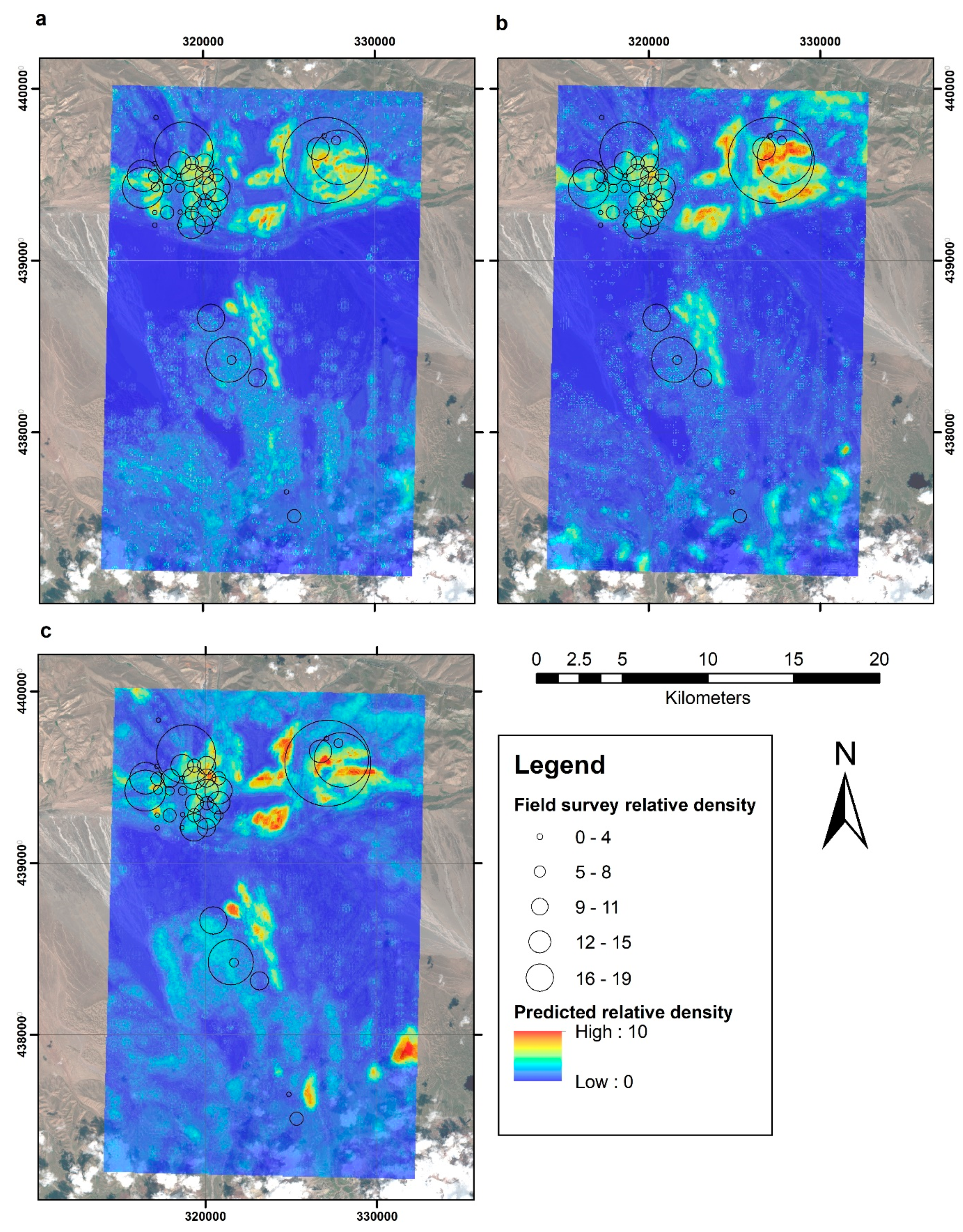
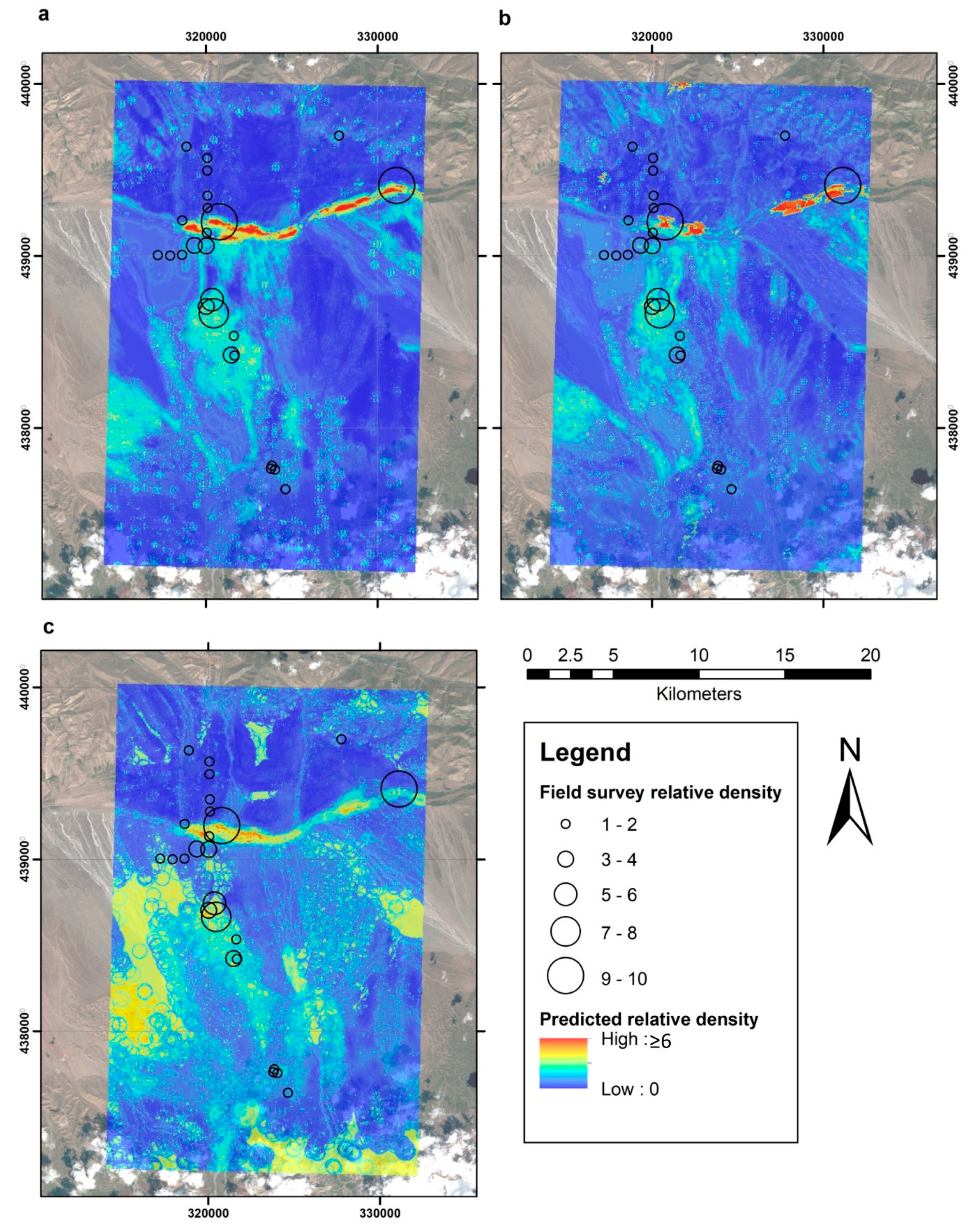
3. Results
4. Discussion
5. Conclusions
Supplementary Materials
Author Contributions
Funding
Conflicts of Interest
References
- Wang, Q.; Raoul, F.; Budke, C.; Craig, P.S.; Xiao, Y.F.; Vuitton, D.A.; Campos-Ponce, M.; Qiu, D.C.; Pleydell, D.R.J.; Giraudoux, P. Grass height and transmission ecology of Echinococcus multilocularis in Tibetan communities, China. Chin. Med. J. 2010, 123, 61–67. [Google Scholar] [PubMed]
- Cheng, Z.; Zhu, S.; Wang, L.; Liu, F.; Tian, H.; Pengsakul, T.; Wang, Y. Identification and characterisation of Emp53, the homologue of human tumor suppressor p53, from Echinococcus multilocularis: Its role in apoptosis and the oxidative stress response. Int. J. Parasitol. 2015, 45, 517–526. [Google Scholar] [CrossRef] [PubMed]
- McManus, D.P.; Zhang, W.; Li, J.; Bartley, P.B. Echinococcosis. Lancet 2003, 362, 1295–1304. [Google Scholar] [CrossRef]
- Torgerson, P.R.; Keller, K.; Magnotta, M.; Ragland, N. The Global Burden of Alveolar Echinococcosis. PLoS Negl. Trop. Dis. 2010, 4, e722. [Google Scholar] [CrossRef] [PubMed]
- Thompson, A.; Deplazes, P.; Lymbery, A. Echinococcus and Echinococcosis; Academic Press: London, UK, 2017. [Google Scholar]
- Massolo, A.; Liccioli, S.; Budke, C.; Klein, C. Echinococcus multilocularis in North America: The great unknown. Parasite 2014, 21, 73. [Google Scholar] [CrossRef] [PubMed]
- Craig, P.S.; Giraudoux, P.; Shi, D.; Bartholomot, B.; Barnish, G.; Delattre, P.; Quéré, J.P.; Harraga, S.; Bao, G.; Wang, Y.H.; et al. An epidemiological and ecological study of human alveolar echinococcosis transmission in south Gansu, China. Acta Trop. 2000, 77, 167–177. [Google Scholar] [CrossRef]
- Giraudoux, P.; Raoul, F.; Pleydell, D.R.J.; Li, T.; Han, X.; Qui, J.; Xie, Y.; Wang, H.; Ito, A.; Craig, P.S. Drivers of Echinococcus multilocularis transmission in China: Small mammal diversity, landscape or climate? PLoS Negl. Trop. Dis. 2013, 7, 1–12. [Google Scholar] [CrossRef]
- Raimkylov, K.M.; Kuttubaev, O.T.; Toigombaeva, V.S. Epidemiological analysis of the distribution of cystic and alveolar echinococcosis in Osh Oblast in the Kyrgyz Republic 2000–2013. J. Helminthol. 2015, 89, 651–654. [Google Scholar] [CrossRef]
- Said-Ali, Z.; Grenouillet, F.; Knapp, J.; Bresson-Hadni, S.; Vuitton, D.A.; Raoul, F.; Richou, C.; Millon, L.; Giraudoux, P. The FrancEchino Network. Detecting nested clusters of human alveolar echinococcosis. Parasitology 2013, 140, 1693–1700. [Google Scholar] [CrossRef]
- Wang, Q.; Yu, W.; Shang, J.; Huang, L.; Mastin, A.; Renqingpengcuo, H.Y.; Zhang, G.; He, W.; Giraudoux, P.; Wu, W.; et al. Seasonal pattern of Echinococcus re-infection in owned dogs in Tibetan communities of Sichuan, China and its implications for control. Infect. Dis. Poverty 2016, 5, 60. [Google Scholar] [CrossRef]
- Nunnari, G.; Pinzone, M.R.; Gruttadauria, S.; Celesia, B.M.; Madeddu, G.; Malaguarnera, G.; Pavone, P.; Cappellani, A.; Cacopardo, B. Hepatic echinococcosis: Clinical and therapeutic aspects. World J. Gastroenterol. 2012, 18, 1448–1458. [Google Scholar] [CrossRef] [PubMed]
- Giraudoux, P.; Craig, P.S.; Delattre, P.; Bao, G.; Bartholomot, B.; Harraga, S.; Quéré, J.P.; Raoul, F.; Wang, Y.; Shi, D.Z.; et al. Interactions between landscape changes and host communities can regulate Echinococcus multilocularis transmission. Parasitology 2003, 127, 121–131. [Google Scholar] [CrossRef]
- Marston, C.G.; Danson, F.M.; Armitage, R.P.; Giraudoux, P.; Pleydell, D.R.J.; Wang, Q.; Qiu, J.; Craig, P.S. A random forest approach to describing Echinococcus multilocularis reservoir Ochotona spp. presence in relation to landscape characteristics in western China. Appl. Geogr. 2014, 55, 176–183. [Google Scholar]
- Raoul, F.; Pleydell, D.R.J.; Quéré, J.P.; Vaniscotte, A.; Rieffel, D.; Takahashi, K.; Bernard, N.; Wang, J.L.; Dobigny, T.; Galbreath, K.E.; et al. Small-mammal assemblage response to deforestation and afforestation in central China. Mammalia 2008, 72, 320–332. [Google Scholar] [CrossRef]
- Giraudoux, P.; Delattre, P.; Habert, M.; Quéré, J.P.; Deblay, S.; Defaut, R.; Duhamel, R.; Moissenet, M.F.; Salvi, D.; Truchetet, D. Population dynamics of fossorial water vole (Arvicola terrestris scherman): A land use and landscape perspective. Agric. Ecosyst. Environ. 1997, 66, 47–60. [Google Scholar] [CrossRef]
- Lidicker, W.Z. Landscape Approaches in Mammalian Ecology and Conservation; University of Minnesota Press: Minneapolis, MN, USA, 1995. [Google Scholar]
- Herbreteau, V.; Demoraes, F.; Khaungaew, W.; Hugot, J.P.; Gonzalez, J.P.; Kittayapong, P.; Souris, M. Use of geographic information system and remote sensing for assessing environment influence on leptospirosis incidence, Phrae province, Thailand. Int. J. Geoinform. 2006, 2, 43–49. [Google Scholar]
- Porcasi, X.; Calderón, G.; Lamfri, M.; Gardenal, N.; Polop, J.; Sabattini, M.; Scavuzzo, C.M. The use of satellite data in modeling population dynamics and prevalence of infection in the rodent reservoir of Junin virus. Ecol. Model. 2005, 185, 437–449. [Google Scholar] [CrossRef]
- Boone, J.D.; McGwire, K.C.; Otteson, E.W.; DeBaca, R.S.; Kuhn, E.A.; Villard, P.; Brussard, P.F.; St Jeor, S.C. Remote sensing and geographic information systems: Charting Sin Nombre virus infections in deer mice. Emerg. Infect. Dis. 2000, 6, 248–258. [Google Scholar] [CrossRef]
- Glass, G.E.; Cheek, J.E.; Patz, J.A.; Shields, T.M.; Doyle, T.J.; Thoroughman, D.A.; Hunt, D.K.; Enscore, R.E.; Gage, K.L.; Irland, C.; et al. Using remotely sensed data to identify areas of risk for hantavirus pulmonary syndrome. Emerg. Infect. Dis. 2000, 63, 238–247. [Google Scholar] [CrossRef]
- Goodin, D.G.; Koch, D.E.; Owen, R.D.; Chu, Y.; Hutchinson, J.S.; Jonsson, C.B. Land cover associated with hantavirus presence in Paraguay. Glob. Ecol. Biogeogr. 2006, 15, 519–527. [Google Scholar] [CrossRef]
- Wayant, N.M.; Maldonado, D.; Rojas de Arias, A.; Cousiño, B.; Goodin, D.G. Correlation between normalized difference vegetation index and malaria in a subtropical rain forest undergoing rapid anthropogenic alteration. Geospat. Health 2010, 4, 179–190. [Google Scholar] [CrossRef] [PubMed]
- Danson, F.M.; Craig, P.S.; Man, W.; Shi, D.Z.; Giraudoux, P. Landscape dynamics and risk modelling of human alveolar echinococcosis. Photogramm. Eng. Remote Sens. 2004, 70, 359–366. [Google Scholar] [CrossRef]
- Giraudoux, P.; Raoul, F.; Afonso, E.; Zaidinov, I.; Yang, Y.; Li, L.; Li, T.; Quere, J.-P.; Feng, X.; Wang, Q.; et al. Transmission ecosystems of Echinococcus multilocularis in China and Central Asia. Parasitology 2013, 140, 1655–1666. [Google Scholar] [CrossRef] [PubMed]
- Danson, F.M.; Graham, A.J.; Pleydell, D.R.J.; Campos-Ponce, M.; Giraudoux, P.; Craig, P.S. Multi-scale spatial analysis of human alveolar echinococcosis risk in China. Parasitology 2003, 127, S133–S141. [Google Scholar] [CrossRef] [PubMed]
- Pleydell, D.R.J.; Yang, Y.R.; Danson, F.M.; Raoul, F.; Craig, P.S.; McManus, D.P.; Vuitton, D.A.; Wang, Q.; Giraudoux, P. Landscape composition and spatial prediction of alveolar echinococcosis in Southern Ningxia, China. PLoS Negl. Trop. Dis. 2008, 2, e287. [Google Scholar] [CrossRef] [PubMed]
- Marston, C.G.; Giraudoux, P.; Armitage, R.P.; Danson, F.M.; Reynolds, S.; Wang, Q.; Qiu, J.; Craig, P.S. Vegetation phenology and habitat discrimination: Impacts for E. multilocularis transmission host modelling. Remote Sens Environ. 2016, 176, 320–327. [Google Scholar] [CrossRef]
- Delattre, P.; Giraudoux, P.; Baudry, J.; Truchetet, D.; Musard, P.; Toussaint, M.; Stahl, P.; Poule, M.L.; Artois, M.; Damange, J.P.; et al. Land use patterns and types of common vole (Microtus arvalis) population kinetics. Agric. Ecosyst. Environ. 1992, 39, 153–169. [Google Scholar] [CrossRef]
- Cao, L.; Cova, T.J.; Dennison, P.E.; Dearing, M.D. Using MODIS satellite imagery to predict hantavirus risk. Glob. Ecol. Biogeogr. 2011, 20, 620–629. [Google Scholar] [CrossRef]
- Zhang, X.; Friedl, M.A.; Schaaf, C.B.; Strahler, A.H.; Hodges, J.C.F.; Gao, F.; Reed, B.C.; Huete, A. Monitoring vegetation phenology using MODIS. Remote Sens. Environ. 2003, 84, 471–475. [Google Scholar] [CrossRef]
- Yu, X.; Zhuang, D.; Chen, H.; Hou, X. Forest classification based on MODIS time series and vegetation phenology. In Proceedings of the International Geoscience and Remote Sensing Symposium, Anchorage, AK, USA, 20–24 September 2004; pp. 2369–2372. [Google Scholar]
- Whelan, T.; Siqueira, P. Time-series classification of Sentinel-1 agricultural data over North Dakota. Remote Sens. Lett. 2018, 9, 411–420. [Google Scholar] [CrossRef]
- Kontgis, C.; Warren, M.S.; Skillman, S.W.; Chartrand, R.; Moody, D.I. Leveraging Sentinel-1 time-series data for mapping agricultural land cover and land use in the tropics. In Proceedings of the 9th International Workshop on the Analysis of Multi Temporal Remote Sensing Images (MultiTemp), Brugge, Belgium, 27–29 June 2017. [Google Scholar]
- Zhou, T.; Pan, J.; Zhang, P.; Wei, S.; Han, T. Mapping winter wheat with multi-temporal SAR and optical images in an urban agricultural region. Sensors 2017, 17, 1210. [Google Scholar] [CrossRef] [PubMed]
- Balzter, H.; Cole, B.; Thiel, C.; Schmullius, C. Mapping CORINE Land Cover from Sentinel-1A SAR and SRTM digital elevation model data using random forests. Remote Sens. 2015, 7, 14876–14898. [Google Scholar] [CrossRef]
- Clerici, N.; Calderón, C.A.V.; Posada, J.M. Fusion of Sentinel-1A and Sentinel-2A data for land cover mapping: A case study in the lower Magdalena region, Colombia. J. Maps 2017, 13, 718–726. [Google Scholar] [CrossRef]
- Ali, M.Z.; Qazi, W.; Aslam, N. A comparative study of ALOS-2 PALSAR and landsat-8 imagery for land cover classification using maximum likelihood classifier. Egypt. J. Remote Sens. Space Sci. 2018, 21, S29–S35. [Google Scholar] [CrossRef]
- Herold, M.; Woodcock, C.; Di Gregorio, A.; Mayaux, P.; Belward, A.; Latham, J.; Schmullius, C.C. A joint initiative for harmonization and validation of land cover datasets. IEEE Trans. Geosci. Remote 2006, 44, 1719–1727. [Google Scholar] [CrossRef]
- De Alban, J.D.T.; Connette, G.M.; Oswald, P.; Webb, E.L. Combined Landsat and L-Band SAR Data Improves Land Cover Classification and Change Detection in Dynamic Tropical Landscapes. Remote Sens. 2018, 10, 306. [Google Scholar] [CrossRef]
- Kussul, N.; Skakun, S.; Shelestov, A.; Kravchenko, O.; Kussul, O. Crop Classification in Ukraine Using Satellite Optical and Sar Images. Int. J. Inf. Models Anal. 2013, 2, 118–122. [Google Scholar]
- Skakun, S.; Kussul, N.; Shelestov, A.Y.; Lavreniuk, M.; Kussul, O. Efficiency Assessment of Multitemporal C-Band Radarsat-2 Intensity and Landsat-8 Surface Reflectance Satellite Imagery for Crop Classification in Ukraine. IEEE J.-STARS 2015, 9, 1–8. [Google Scholar] [CrossRef]
- Kou, W.; Xiao, X.; Dong, J.; Gan, S.; Zhai, D.; Zhang, G.; Qin, Y.; Li, L. Mapping deciduous rubber plantation areas and stand ages with PALSAR and Landsat images. Remote Sens. 2015, 7, 1048–1073. [Google Scholar] [CrossRef]
- Qin, Y.; Xiao, X.; Dong, J.; Zhang, G.; Roy, P.S.; Joshi, P.K.; Gilani, H.; Murthy, M.S.R.; Jin, C.; Wang, J.; et al. Mapping forests in monsoon Asia with ALOS PALSAR 50-m mosaic images and MODIS imagery in 2010. Sci. Rep. 2016, 6, 570. [Google Scholar] [CrossRef]
- Reiche, J.; Souza, C.M.; Hoekman, D.H.; Verbesselt, J.; Persaud, H.; Herold, M. Feature level fusion of multi-temporal ALOS PALSAR and Landsat data for mapping and monitoring of tropical deforestation and forest degradation. IEEE J.-STARS 2013, 6, 2159–2173. [Google Scholar] [CrossRef]
- Reiche, J.; Verbesselt, J.; Hoekman, D.; Herold, M. Fusing Landsat and SAR time series to detect deforestation in the tropics. Remote Sens Environ. 2015, 156, 276–293. [Google Scholar] [CrossRef]
- Erasmi, S.; Twele, A. Regional land over mapping in the humid tropics using combined optical and SAR satellite data—A case study from Central Sulawesi, Indonesia. Int. J. Remote Sens. 2009, 30, 2465–2478. [Google Scholar] [CrossRef]
- Gessner, U.; Machwitz, M.; Esch, T.; Tillack, A.; Naeimi, V.; Kuenzer, C.; Dech, S. Multi-sensor mapping of West African land cover using MODIS, ASAR and TanDEM-X/TerraSAR-X data. Remote Sens. Environ. 2015, 164, 282–297. [Google Scholar] [CrossRef]
- Jhonnerie, R.; Siregar, V.P.; Nababan, B.; Prasetyo, L.B.; Wouthuyzen, S. Random Forest classification for mangrove land cover mapping using Landsat 5 TM and ALOS PALSAR imageries. Procedia Environ. Sci. 2015, 24, 215–221. [Google Scholar] [CrossRef]
- Torbick, N.; Ledoux, L.; Salas, W.; Zhao, M. Regional mapping of plantation extent using multisensor imagery. Remote Sens. 2016, 8, 236. [Google Scholar] [CrossRef]
- Vaglio Laurin, G.; Liesenberg, V.; Chen, Q.; Guerriero, L.; Del Frate, F.; Bartolini, A.; Coomes, D.; Wilebore, B.; Lindsell, J.; Valentini, R. Optical and SAR sensor synergies for forest and land cover mapping in a tropical site in West Africa. Int. J. Appl. Earth Obs. Geoinf. 2013, 21, 7–16. [Google Scholar] [CrossRef]
- Wijaya, A.; Gloaguen, R. Fusion of ALOS PALSAR and Landsat ETM data for land cover classification and biomass modeling using non-linear methods. In Proceedings of the 2009 International Geoscience and Remote Sensing Symposium (IGARSS), Cape Town, South Africa, 12–17 July 2009; Volume 3, pp. 581–584. [Google Scholar]
- Rüetschi, M.; Schaepman, M.E.; Small, D. Using Multitemporal Sentinel-1 C-band Backscatter to Monitor Phenology and Classify Deciduous and Coniferous Forests in Northern Switzerland. Remote Sens. 2018, 10, 55. [Google Scholar] [CrossRef]
- Minh, H.L.; Truong, V.; Duong, N.D.; Anh, T.T. Identification of land cover features phenology using multi-temporal Sentinel-1 data: A case study in Hanoi, Vietnam. In Proceedings of the 37th Asian Conference on Remote Sensing, Colombo, Sri Lanka, 17–21 October 2016. [Google Scholar]
- Afonso, E.; Knapp, J.; Tete, N.; Umhang, G.; Rieffel, D.; van Kesteren, F.; Ziadinov, I.; Craig, P.S.; Torgerson, P.R.; Giraudoux, P. Echinococcus multilocularis in Kyrgyzstan: Similarity in the Asian EmsB genotypic profiles from village populations of Eastern mole voles (Ellobius tancrei) and dogs in the Alay valley. J. Helminthol. 2015, 89, 664–670. [Google Scholar] [CrossRef]
- Raoul, F.; Quere, J.P.; Rieffel, D.; Bernard, N.; Takahashi, K.; Scheifler, R.; Wang, Q.; Qiu, J.; Yang, W.; Craig, P.S.; et al. Distribution of small mammals in a pastoral landscape of the Tibetan plateau (Western Sichuan, China) and relationship with grazing practices. Mammalia 2006, 42, 214–225. [Google Scholar]
- Giraudoux, P.; Quere, J.P.; Delattre, P.; Bao, G.; Wang, X.; Shi, D.; Vuitton, D.; Craig, P.S. Distribution of small mammals along a deforestation gradient in south Gansu, China. Acta Theriol. 1998, 43, 349–362. [Google Scholar] [CrossRef]
- Delattre, P.; Giraudoux, P.; Damange, J.P.; Quere, J.P. Recherche d’un indicateur de la cinétique démographique des populations du Campagnol des champs (Microtus arvalis). Rev. Ecol. 1990, 45, 375–384. [Google Scholar]
- Giraudoux, P.; Pradier, B.; Delattre, P.; Deblay, S.; Salvi, D.; Defaut, R. Estimation of water vole abundance by using surface indices. Acta Theriol. 1995, 40, 77–96. [Google Scholar] [CrossRef]
- McNemar, Q. Note on the sampling error of the difference between correlated proportions or percentages. Psychometrika 1947, 12, 153–157. [Google Scholar] [CrossRef] [PubMed]
- Momeni, R.; Aplin, P.; Boyd, D.S. Mapping complex urban land cover from spaceborne imagery: The influence of spatial resolution, spectral band set and classification approach. Remote Sens. 2016, 8, 88. [Google Scholar] [CrossRef]
- Giraudoux, P.; Delattre, P.; Takahashi, K.; Raoul, F.; Quere, J.P.; Craig, P.S.; Vuitton, D. Transmission ecology of Echinococcus multilocularis in wildlife: What can be learned from comparative studies and multiscale approaches? In Cestode Zoonoses: Echinococcosis and Cysticercosis: An Emergent and Global Problem, 341st ed.; Craig, P., Pawlowski, Z., Eds.; IOS Press: Amsterdam, The Netherlands, 2002; pp. 251–266. [Google Scholar]
- Pleydell, D.R.; Raoul, F.; Tourneux, F.; Danson, F.M.; Graham, A.J.; Craig, P.S.; Giraudoux, P. Modelling the spatial distribution of Echinococcus multilocularis infection in foxes. Acta Trop. 2004, 91, 253–265. [Google Scholar] [CrossRef] [PubMed]
- Liccioli, S.; Giraudoux, P.; Deplazes, P.; Massolo, A. Wilderness in the “city” revisited: Different urbes shape transmission of Echinococcus multilocularis by altering predator and prey communities. Trends Parasitol. 2015, 31, 297–305. [Google Scholar] [CrossRef]
- Rhodes, J.R.; McAlpine, C.A.; Zuur, A.F.; Smith, G.M.; Ieno, E.N. GLMM Applied on the Spatial Distribution of Koalas in a Fragmented Landscape. Mixed Effects Models and Extensions in Ecology with R (pp. 469e492); Zuur, A.F., Ieno, E.N., Walker, N.J., Saveliev, A.A., Smith, G.M., Eds.; Springer: New York, NY, USA, 2009. [Google Scholar]
- Breiman, L. Random forests. Mach. Learn. 2001, 45, 5–32. [Google Scholar] [CrossRef]
- Cutler, D.R.; Edwards, T.C., Jr.; Beard, K.H.; Cutler, A.; Hess, K.T.; Gibson, J.; Lawler, J.J. Random forests for classification in ecology. Ecology 2007, 88, 2783–2792. [Google Scholar] [CrossRef]
- Svetnik, V.; Liaw, A.; Tong, C.; Culberson, J.C.; Sheridan, R.P.; Feuston, B.P. Random Forests: A classification and regression tool for compound classification and QSAR modeling. J. Chem. Inf. Model. 2003, 43, 1947–1958. [Google Scholar] [CrossRef]
- Strobl, C.; Boulesteix, A.L.; Kneib, T.; Augustin, T.; Zeileis, A. Conditional variable importance for random forests. BMC Bioinf. 2008, 9, 307. [Google Scholar] [CrossRef] [PubMed]
- Duro, D.C.; Franklin, S.E.; Dube, M.G. Multi-scale object-based image analysis and feature selection of multi-sensor earth observation imagery using random forests. Int. J. Remote Sens. 2012, 33, 4502–4526. [Google Scholar] [CrossRef]
- Perdiguero-Alonso, D.; Montero, F.E.; Kostadinova, A.; Raga, J.A.; Barrett, J. Random forests, a novel approach for discrimination of fish populations using parasites as biological tags. Int. J. Parasitol. 2008, 38, 1425–1434. [Google Scholar] [CrossRef] [PubMed]
- Marston, C.G.; Wilkinson, D.M.; Reynolds, S.C.; Louys, J.; O’Regan, H.J. Water availability is a principle driver of large-scale land cover spatial heterogeneity in sub-Saharan savannahs. Landsc. Ecol. 2018, 1–15. [Google Scholar] [CrossRef]
- Ryo, M.; Rillig, M.C. Statistically reinforced machine learning for nonlinear patterns and variable interactions. Ecosphere 2017, 8, e01976. [Google Scholar] [CrossRef]
- Veldhuis, M.P.; Rozen-Rechels, D.; le Roux, E.; Cromsigt, J.P.G.M.; Berg, M.P.; Olff, H. Determinants of patchiness of woody vegetation in an African savanna. J. Veg. Sci. 2016, 28, 93–104. [Google Scholar] [CrossRef]
- Liaw, A.; Wiener, M. Classification and regression by randomForest. R News 2002, 2, 18–22. [Google Scholar]
- Giraudoux, P.; Pleydell, D.; Raoul, F.; Quere, J.P.; Qian, W.; Yang, Y.; Vuitton, D.A.; Qiu, J.M.; Yang, W.; Craig, P.S. Echinococcus multilocularis: Why are multidisciplinary and multiscale approaches essential in infectious disease ecology? Trop Med. Health 2007, 55, S237–S246. [Google Scholar] [CrossRef]
- Krebs, C.J. Population Fluctuations in Rodents; The University of Chicago Press: Chicago, IL, USA; London, UK, 2013. [Google Scholar]


| Number | Satellite | Date | Orbit |
|---|---|---|---|
| 1 | Sentinel-1A | 18 October 2014 | Descending |
| 2 | Sentinel-1A | 24 October 2014 | Ascending |
| 3 | Sentinel-1A | 11 November 2014 | Descending |
| 4 | Sentinel-1A | 17 November 2014 | Ascending |
| 5 | Sentinel-1A | 5 December 2014 | Descending |
| 6 | Sentinel-1A | 11 December 2014 | Ascending |
| 7 | Sentinel-1A | 29 December 2014 | Descending |
| 8 | Sentinel-1A | 4 January 2015 | Ascending |
| 9 | Sentinel-1A | 22 January 2015 | Descending |
| 10 | Sentinel-1A | 15 February 2015 | Descending |
| 11 | Sentinel-1A | 21 February 2015 | Ascending |
| 12 | Sentinel-1A | 27 February 2015 | Descending |
| 13 | Sentinel-1A | 17 March 2015 | Ascending |
| 14 | Sentinel-1A | 23 March 2015 | Descending |
| 15 | Sentinel-1A | 10 April 2015 | Ascending |
| 16 | Sentinel-1A | 4 May 2015 | Ascending |
| 17 | Sentinel-1A | 3 June 2015 | Descending |
| 18 | Sentinel-1A | 21 June 2015 | Ascending |
| 19 | Sentinel-1A | 27 June 2015 | Descending |
| 20 | Sentinel-1A | 15 July 2015 | Ascending |
| 21 | Sentinel-1A | 21 July 2015 | Descending |
| 22 | Sentinel-1A | 8 August 2015 | Ascending |
| 23 | Sentinel-1A | 14 August 2015 | Descending |
| 24 | Sentinel-1A | 1 September 2015 | Ascending |
| 25 | Sentinel-1A | 7 September 2015 | Descending |
| 26 | Sentinel-1A | 25 September 2015 | Ascending |
| 27 | Sentinel-1A | 1 October 2015 | Descending |
| 28 | Sentinel-1A | 19 October 2015 | Ascending |
| 29 | Landsat OLI | 22 July 2014 |
| SAR and OLI | SAR-Only | OLI-Only | ||||
|---|---|---|---|---|---|---|
| Land Cover Class | UA (%) | PA (%) | UA (%) | PA (%) | UA (%) | PA (%) |
| Built up | 94.74 | 72.00 | 95.24 | 80.00 | 72.00 | 72.00 |
| Bare | 85.71 | 96.00 | 83.05 | 98.00 | 82.35 | 84.00 |
| Water | 100.00 | 97.37 | 100.00 | 76.32 | 88.10 | 97.37 |
| Dry grassland | 89.29 | 100.00 | 85.96 | 98.00 | 92.59 | 100.00 |
| Alpine grassland | 98.04 | 100.00 | 97.96 | 96.00 | 98.00 | 98.00 |
| Steppe | 97.87 | 92.00 | 86.27 | 88.00 | 97.83 | 90.00 |
| Bushes | 97.22 | 89.74 | 97.37 | 94.87 | 92.31 | 61.54 |
| Agriculture | 98.00 | 98.00 | 91.67 | 88.00 | 82.76 | 96.00 |
| SAR and OLI | SAR-Only | OLI-Only | ||||
|---|---|---|---|---|---|---|
| Importance Ranking | Variable | p-Value | Variable | p-Value | Variable | p-Value |
| 1 | AG 100 m ** | 0.001 (16.778) | AG 250 m ** | <0.001 (17.924) | AG 150 m ** | 0.001 (17.187) |
| 2 | AG 150 m ** | 0.005 (14.300) | AG 100 m ** | 0.005 (15.603) | AG 300 m ** | 0.001 (16.200) |
| 3 | AG 200 m * | 0.016 (13.478) | AG 300 m ** | 0.009 (15.562) | AG 200 m ** | 0.001 (16.137) |
| 4 | AG 300 m * | 0.015 (13.308) | AG 350 m * | 0.023 (12.557) | AG 250 m ** | 0.002 (13.392) |
| 5 | AG 250 m * | 0.039 (11.696) | AG 150 m * | 0.021 (11.416) | AG 100 m ** | 0.002 (13.242) |
| 6 | DG 350 m | 0.067 (11.657) | BU 450 m * | 0.018 (10.104) | AG 50 m ** | 0.004 (12.807) |
| 7 | AG 500 m * | 0.042 (11.523) | AG 200 m * | 0.041 (9.683) | AG 350 m ** | 0.006 (12.790) |
| 8 | AG 400 m * | 0.036 (10.900) | AG 400 m | 0.092 (9.239) | AG 450 m ** | 0.010 (12.771) |
| 9 | AG 450 m | 0.053 (9.587) | BU 500 m * | 0.046 (9.237) | AG 500 m * | 0.013 (11.952) |
| 10 | DG 300 m | 0.155 (9.370) | AG 500 m | 0.082 (8.878) | BU 400 m ** | 0.007 (11.685) |
| 11 | AG 50 m * | 0.033 (9.325) | AG 450 m | 0.173 (8.818) | AG 400 m * | 0.025 (11.420) |
| 12 | AG 350 m | 0.096 (9.307) | BA 500 m | 0.179 (7.659) | BU 500 m * | 0.031 (10.545) |
| 13 | BU 500 m | 0.063 (8.912) | BU 300 m | 0.113 (7.163) | AP 200 m | 0.057 (8.525) |
| 14 | DG 400 m | 0.317 (8.663) | BU 250 m | 0.128 (7.016) | BU 300 m | 0.104 (7.551) |
| 15 | DG 500 m | 0.369 (8.316) | DG 100 m | 0.280 (6.938) | BU 450 m | 0.123 (7.503) |
| SAR and OLI | SAR-Only | OLI-Only | ||||
|---|---|---|---|---|---|---|
| Importance Ranking | Variable | p-Value | Variable | p-Value | Variable | p-Value |
| 1 | BS 50 m ** | 0.001 (13.673) | AG 450 m ** | 0.006 (22.610) | BS 300 m ** | 0.002 (14.649) |
| 2 | ST 350 m | 0.217 (10.539) | WA 200 m * | 0.038 (9.083) | ST 500 m | 0.079 (13.446) |
| 3 | ST 400 m | 0.278 (10.443) | ST 350 m | 0.226 (7.801) | AG 500 m | 0.201 (10.848) |
| 4 | ST 450 m | 0.338 (8.961) | ST 300 m | 0.238 (6.696) | ST 300 m | 0.241 (8.914) |
| 5 | BS 100 m ** | 0.006 (8.761) | ST 500 m | 0.295 (6.319) | DG 300 m | 0.413 (8.151) |
| 6 | BS 300 m * | 0.032 (8.452) | ST 450 m | 0.355 (5.791) | DG 400 m | 0.465 (7.978) |
| 7 | ST 500 m | 0.416 (8.273) | WA 350 m | 0.138 (5.558) | DG 450 m | 0.466 (7.947) |
| 8 | AP 200 m | 0.152 (8.192) | ST 400 m | 0.446 (5.544) | ST 250 m | 0.278 (7.849) |
| 9 | DG 200 m | 0.722 (8.074) | AG 500 m | 0.402 (5.428) | DG 500 m | 0.478 (7.807) |
| 10 | BS 400 m | 0.103 (7.846) | BS 300 m | 0.200 (5.106) | DG 100 m | 0.489 (7.744) |
| 11 | DG 300 m | 0.772 (7.124) | ST 250 m | 0.453 (4.761) | DG 350 m | 0.636 (6.697) |
| 12 | ST 300 m | 0.498 (7.123) | BU 500 m | 0.257 (4.621) | AG 250 m | 0.432 (6.246) |
| 13 | DG 50 m | 0.549 (6.629) | BS 50 m * | 0.035 (4.154) | AG 300 m | 0.457 (6.242) |
| 14 | BS 350 m | 0.121 (6.386) | WA 400 m | 0.269 (4.121) | DG 200 m | 0.649 (5.294) |
| 15 | DG 100 m | 0.717 (6.359) | WA 250 m | 0.175 (4.035) | AP 500 m | 0.419 (4.764) |
© 2018 by the authors. Licensee MDPI, Basel, Switzerland. This article is an open access article distributed under the terms and conditions of the Creative Commons Attribution (CC BY) license (http://creativecommons.org/licenses/by/4.0/).
Share and Cite
Marston, C.; Giraudoux, P. On the Synergistic Use of Optical and SAR Time-Series Satellite Data for Small Mammal Disease Host Mapping. Remote Sens. 2019, 11, 39. https://doi.org/10.3390/rs11010039
Marston C, Giraudoux P. On the Synergistic Use of Optical and SAR Time-Series Satellite Data for Small Mammal Disease Host Mapping. Remote Sensing. 2019; 11(1):39. https://doi.org/10.3390/rs11010039
Chicago/Turabian StyleMarston, Christopher, and Patrick Giraudoux. 2019. "On the Synergistic Use of Optical and SAR Time-Series Satellite Data for Small Mammal Disease Host Mapping" Remote Sensing 11, no. 1: 39. https://doi.org/10.3390/rs11010039
APA StyleMarston, C., & Giraudoux, P. (2019). On the Synergistic Use of Optical and SAR Time-Series Satellite Data for Small Mammal Disease Host Mapping. Remote Sensing, 11(1), 39. https://doi.org/10.3390/rs11010039