Object-Based Plastic-Mulched Landcover Extraction Using Integrated Sentinel-1 and Sentinel-2 Data

Abstract

Plastic mulching on farmland has been increasing worldwide for decades due to its superior advantages for improving crop yields. Monitoring Plastic-Mulched Land-cover (PML) can provide essential information for making agricultural management decisions and reducing PML’s eco-environmental impacts. However, mapping PML with remote sensing data is still challenging and problematic due to its complicated and mixed characteristics. In this study, a new Object-Based Image Analysis (OBIA) approach has been proposed to investigate the potential for combined use of Sentinel-1 (S1) SAR and Sentinel-2 (S2) Multi-spectral data to extract PML. Based on the ESP2 tool (Estimation of Scale Parameter 2) and ED2 index (Euclidean Distance 2), the optimal Multi-Resolution Segmentation (MRS) result is chosen as the basis of following object-based classification. Spectral and backscattering features, index features and texture features from S1 and S2 are adopted in classifying PML and other land-cover types. Three machine-learning classifiers known as the—Classification and Regression Tree (CART), the Random Forest (RF) and the Support Vector Machine (SVM) are carried out and compared in this study. The best classification result with an overall accuracy of 94.34% is achieved by using spectral, backscattering, index and textural information from integrated S1 and S2 data with the SVM classifier. Texture information is demonstrated to contribute positively to PML classifications with SVM and RF classifiers. PML mapping using SAR information alone has been greatly improved by the object-based approach to an overall accuracy of 87.72%. By adding SAR data into optical data, the accuracy of object-based PML classifications has also been improved by 1–3%.

1. Introduction

In the past decades, plasticulture has been widely utilized in agriculture around the world due to its notable advantages for improving crop yields by shielding crops from adverse conditions, such as coldness, heat, strong rainfall, wind, drought, harmful insects, and crop diseases, conserving water resources, and increasing the soil temperature [1]. However, plasticulture also has some negative impacts on local or regional eco-environment because it reduces the biodiversity by changing the pollination of plants and deteriorates the soil structure by leaving plastic film residue [2,3].

The raising concerns on plastic waste and pollution and other eco-environmental effects of plasticulture call for further research to respond. Monitoring and mapping plastic-mulched landcover (PML) which is one of the three dominant types of plasticultrue [3] and covers 95% area of overall plasticulture farmland in China [4] can provide prerequisites for improving agricultural management and lessening PML’s eco-environmental impacts. The conventional methods for PML mapping such as field-surveying and photogrammetric measurement are time-consuming, expensive and labor-intensive. In this context, remote sensing techniques are the only promising approaches to acquiring PML information for a large geographic area regardless of time and locations. However, mapping PML automatically with remote sensing data is far from being solved due to PML’s special and mixed characteristics.

Remote-sensing image classification is a widely used technique for plasticulture and other types of land use and land cover detection. In recent years, there has been growing interest in mapping plasticulture farmland using remote sensing data of different spectral and spatial resolutions, but the number of studies in PML is limited. The research on plasticulture landscape extraction can be divided into two main approaches: pixel-based image analysis and object-based image analysis (OBIA). The former are adopted widely on detecting plasticulture information from satellite data at different spatial resolutions [5,6,7,8,9,10,11,12]. For example, Lu et al. mapped the plastic-mulched cotton landcover from Landsat-5 TM and MODIS time series data respectively based on the decision tree model [2,3]. Hasituya et al. extracted the plastic-mulched farmland using Landsat-8 data and using different features [8,9]. Later, Hasituya et al. selected the appropriate spatial scale for mapping plastic-mulched farmland based on the concept of average local variance with GaoFen-1 imagery [10]. The OBIA is mostly used to detect plastic greenhouses from high spatial resolution images. Aguilar et al. utilized stereo pairs acquired from very high-resolution optical satellites GeoEye-1 and WorldView-2 to carry out greenhouse classification and demonstrated the importance of integrating the normalized digital surface model into the classification workflow [13]. They also mapped greenhouses with Landsat-8 time series based on the WorldView-2 segmentation using spectral, textural, seasonal statistics and other indices, and attained an overall accuracy over 93.0% [14]. Novelli et al. evaluated the performance of S2 and Landsat-8 data on object-based greenhouse extraction and compared the classification results based on the segmentation of WorldView-2 [15]. Aguilar et al. assessed the performance of multi-resolution segmentation with different parameter settings for extracting greenhouses from WorldView-2 imagery [16]. Besides extracting greenhouses land cover, Aguilar et al. also considered up an innovative study for identifying greenhouse horticultural crops that grew under plastic coverings with Landsat-8 time series images and reached an overall accuracy of 81.3% [17]. All the research studies mentioned above are about object-based greenhouse extraction. However, the spectral characteristics and the spatial patterns of PML are very different from plastic greenhouses. The OBIA approaches, demonstrated to be more efficient in greenhouse detection than pixel-based ones [18], have not been investigated in PML extraction.

Synthetic Aperture Radar (SAR), which is a type of active microwave remote sensing technique, has several advantages including all-time and all-weather observations and the ability to penetrate cloud and other objects. Because of those advantages, SAR has already been utilized along with optical remote sensing data in many agricultural applications [19,20]. Preliminary studies showed that SAR data might complement optical remote sensing data in PML mapping. For example, Hasituya et al. explored the potential of multi-polarization Radarsat-2 for mapping PML despite its relatively poor classification accuracy below 75% [21].

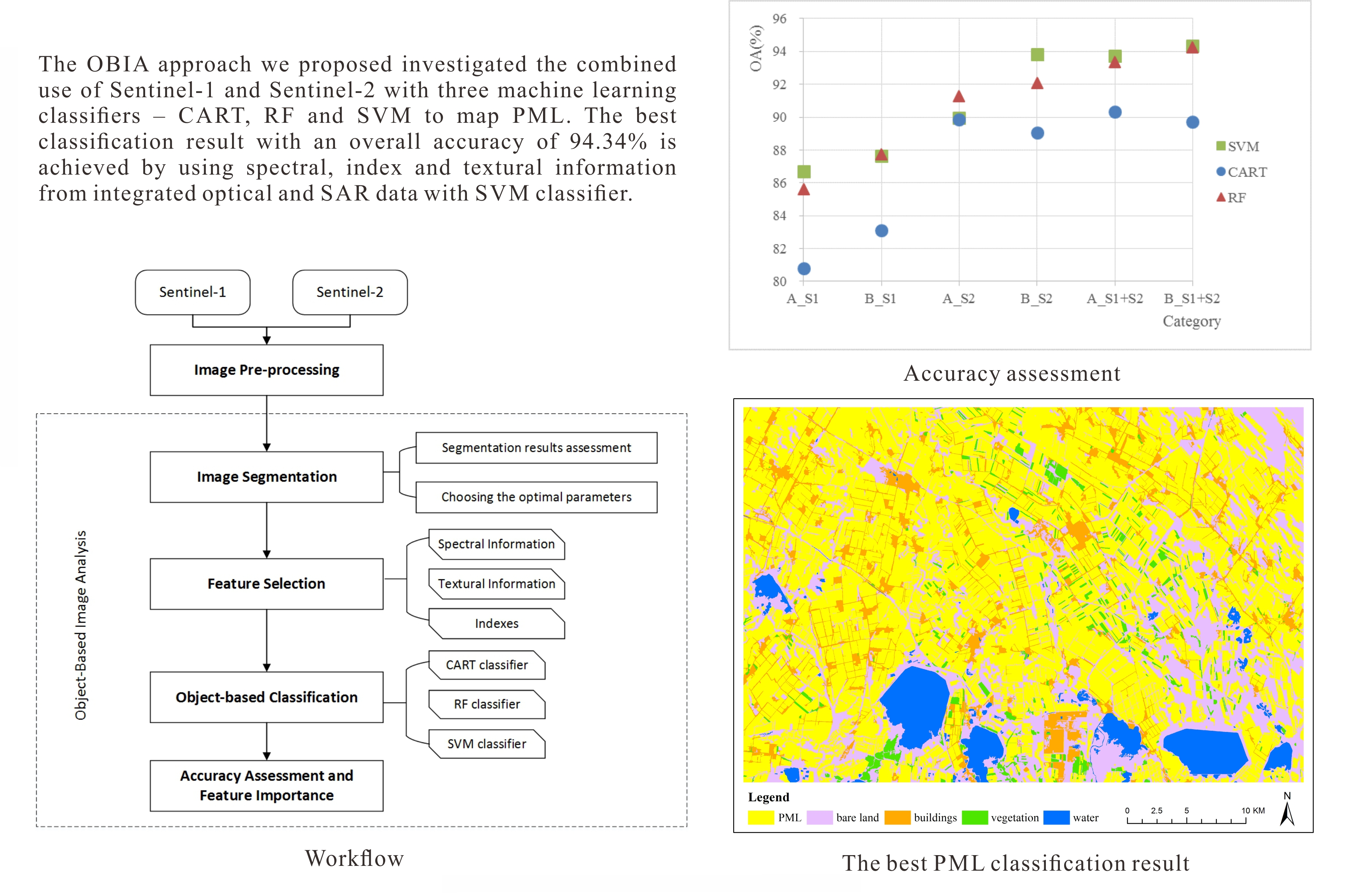
This paper proposed an object-based approach for PML detection using S1 SAR and S2 optical data with three machine learning classifiers: Classification and Regression Tree (CART), Random Forest (RF), and Support Vector Machine (SVM). As far as the authors’ knowledge, this is the first study comparing and integrating optical and SAR data for PML mapping. The main purposes of this study are: (1) to verify the effectiveness of OBIA for PML mapping, (2) to explore the importance of SAR data and evaluate its performance by combining SAR data with optical data in PML detection, and (3) to compare the performance of three machine learning algorithms, CART, RF, and SVM in PML mapping.

2. Study Area and Data Pre-Processing

2.1. Study Area

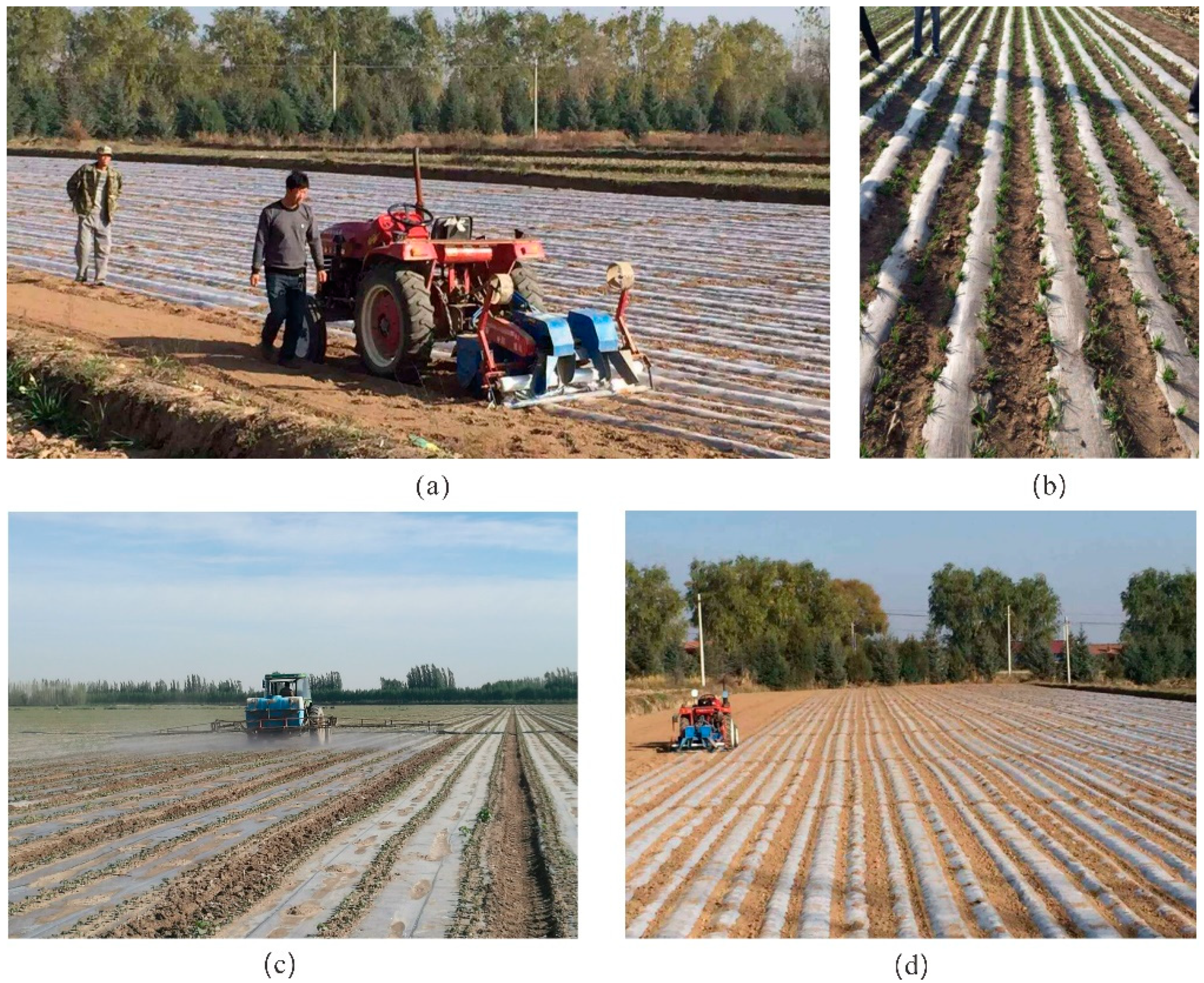
A region in northern Xinjiang, China was chosen as the study area and covered a large area of cotton field where plastic mulching is used 100%. The region is situated in Shihezi City between 44°24′23″N–44°41′12″N and 85°44′19″E–86°20′19″E with an area of over 1500 km² (Figure 1). The region has typical temperate continental arid climate, featuring hot summer and cold winter with great diurnal and annual temperature variations. The study area presents various land-cover types, which include PML (as the major one), bare land, buildings, vegetation and water. The major crops in the area include cotton, wheat and corn, and their planting time ranges from the middle of April to the middle of October. Some photos of PML in the study area are shown in Figure 2. The differences in the PML presence might contribute to the differences of soil conditions, which is the vegetation growing period and, how plastic film is mulched. The PML we investigate is a mixed field compromised of plastic coverings and bare soil. PML field in the study area has an average width of around 100 m.

2.2. Data Pre-Processing

The free availability of Sentinel 1 (S1) SAR and Sentinel 2 (S2) multispectral instrument from European Space Agency gives researchers great opportunities to explore the use of those satellite data on land cover studies. This study used two images including one S1 SAR image and one S2 optical image.

The SAR image is a Sentinel-1B C-band SAR Interferometric Wide Swath (IW) scene in VH and VV polarizations dated from 11 May 2017. The IW mode has a swath width of more than 250 km with a ground-range single look resolution of 5 m × 20 m in range and azimuth directions, respectively [22]. We used the S1 Level-1 Ground Range Detected (GRD) product, which is focused SAR data that has been detected, multi-looked and projected to ground range using an Earth ellipsoid model—WGS 84. GRD products have removed thermal noise and have approximate square pixels with reduced speckles. On 11 May 2017, the weather in the study area, Shihezi City was cloudy with temperatures ranging from 13 °C to 31 °C, and the weather was sometimes sunny, cloudy and rainy before 11 May 2017.

The optical image is a Sentinel-2A Level-1C multispectral scene from 14 May 2017 with less than 5% cloud cover. S2 Level-1C products are ortho-images composed of 100 km² tiles in UTM/WGS84 projection and provide Top-Of-Atmosphere (TOA) reflectance. S2 is a multispectral platform that contains 13 bands with different resolutions of 10 m, 20 m and 60 m. The 10 m-resolution bands are Blue, Green, Red, and Near Infrared, The 20 m-resolution bands are four Vegetation Red Edge bands and two Short-wave Infrared bands, The 60 m-resolution bands are the Coastal Aerosol band, the Water Vapor band, and the Cirrus band.

Since there are only three days apart between the two datasets, we assume that major changes on land cover can be neglected and the two datasets can be employed together. The following pre-processing steps for the two satellite images were conducted. For the SAR image, the S1 GRD IW image was first applied to the orbit filesand then radiometrically calibrated to the radar backscatter sigma0. SAR images have inherent noise speckles caused by random constructive and destructive interference. These noise speckles degrade the quality of the image and make interpretation more difficult. Therefore, a 5 × 5 Lee Sigma Filter [23] was used to reduce speckles. Afterwards, the SAR image was geometrically corrected by applying the Range Doppler Terrain Correction with a 3” SRTM (Shuttle Radar Topography Mission) digital elevation model [24] in order to eliminate inherent SAR geometry effects such as foreshortening, layover and shadow. For the optical image, the S2 L1C image was processed into Level 2A (Note: the cirrus band 10 is excluded since it does not represent surface information.) through atmospheric correction and terrain correction using the Sen2Cor Processor [25]. Both the S1 SAR image and the S2 multispectral image were resampled into a 10 m resolution, and then they were co-registered to create an image stack and were subset into the study area. The whole pre-processing for S1 and S2 was carried out on the platform SNAP from ESA [26].

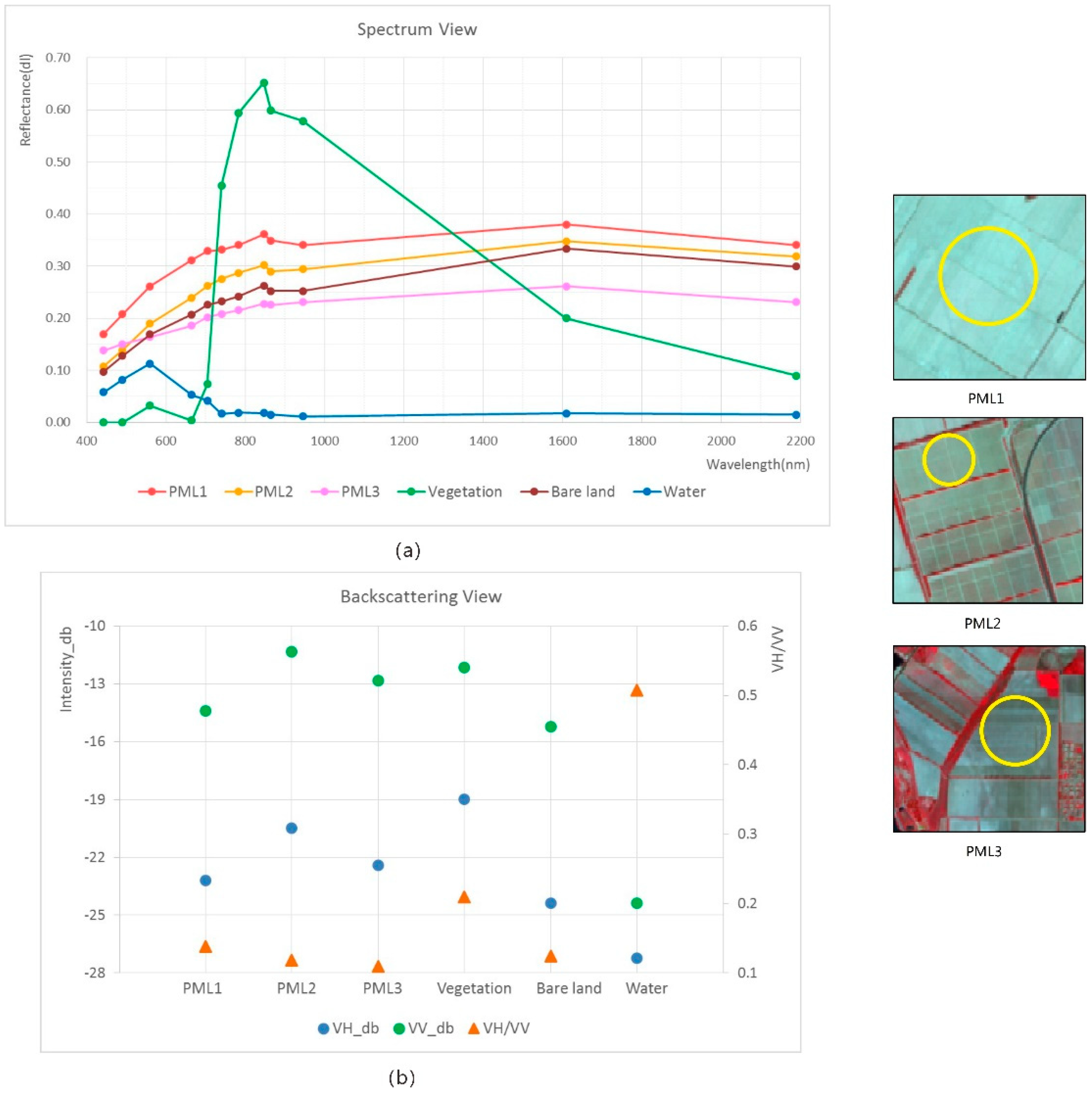
The spectral reflectance and backscattering information of three typical PMLs were explored from S1 and S2 data, which is shown in Figure 3. The spectral reflectance and backscattering intensity values of a certain PML were defined as the median value of the samples of a certain PML we chose. It is shown that different PML presences have very difference spectral and backscattering characteristics.

3. Material and Methods

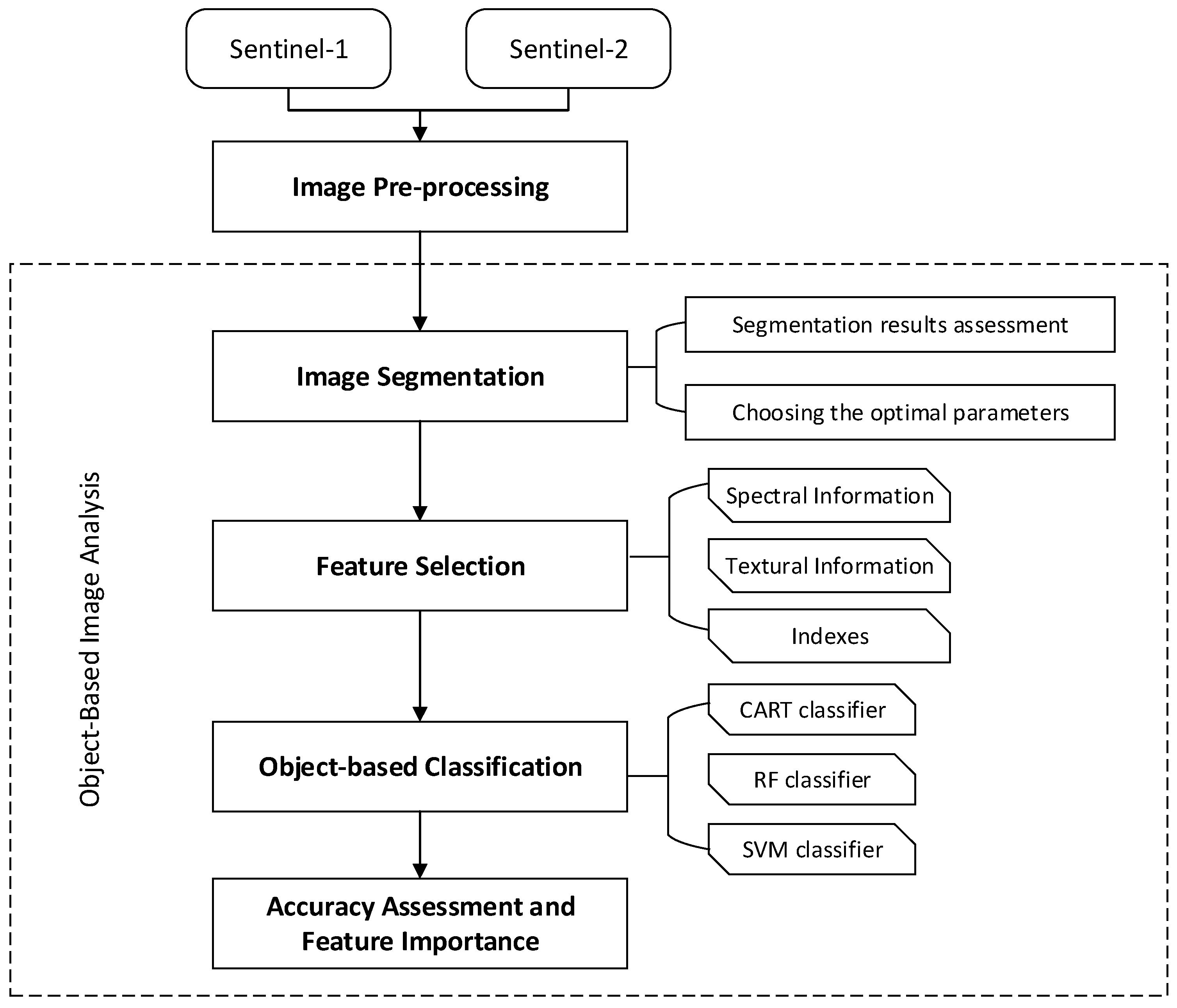
Based on S1 and S2 data, the main methodological procedures are as follows: (1) Segment the satellite images into meaningful objects by using the multi-resolution segmentation algorithm, (2) select appropriate features for mapping PML, (3) based on the optimal segmentation results, conduct object-based classification with a special attention to PML by three machine learning algorithms, and (4) assess the classification accuracy and figure out the important features extracting PML. The overview of the methodology and workflow are presented in Figure 4.

3.1. Multi-Resolution Segmentation

In the workflow of OBIA, image segmentation is the first and critical procedure, which aims to create meaningful objects by dividing an image into intra-homogeneous and inter-heterogeneous regions. Multi-resolution segmentation (MRS) was applied in this study. MRS is a bottom-up region-merging technique starting at random points with one-pixel objects and then merging them into bigger segments [27]. It is a stepwise optimization process with certain constrains on regional minimum heterogeneity. In numerous iterative steps, one-pixel separated objects are merged in pair into small image objects which then form bigger ones in the same way until the constrains on heterogeneity are met. During the region-growing process, the possible growths of the heterogeneity criterion of two adjacent objects are calculated. Then the pair objects are merged with the smallest growth. If the smallest growth exceeds the heterogeneity threshold, which is given by the scale parameter, the iterative procedure stops.

Heterogeneity in MRS comprises color and shape features. Color can be regarded as spectral information or values in the image. The shape is evaluated by two factors—smoothness and compactness. The contribution in heterogeneity by color and shape can be weighted by users. The scale parameter defines the stop criterion of heterogeneity for the optimization process. In general, the larger the scale parameter is, the larger but less homogenous objects will grow in the segmentation. Details and further explanations can be found in References [28,29].

3.2. Scale Parameter Selection and Segmentation Quality Assessment

Different parameter settings in MRS can produce segmentation results of different quality. Therefore, it is very important to choose the best parameter combinations especially the optimal scale parameter in MRS.

We adopted the ESP2 (Estimation of Scale Parameter 2) tool proposed by Dragut et al. to choose the scale parameter of MRS objectively [30,31,32]. The main method of the ESP2 tool is based on the concept of local variance (LV), which can be regarded as a useful indicator to access whether the meaning objects reach their appropriate scale [30]. The LV for a scene of a certain scale is calculated as the average standard deviation of objects obtained through segmentation at the scene level.

In MRS, when the size of a segment increases with the scale parameter, its standard deviation increases accordingly until it represents a meaningful object in the real world. Then, if the scale parameter continues to grow within a certain range where the object can still be distinguished from its background, its standard deviation stagnates. After producing multiple segmentations on the same dataset by increasing the scale parameter incrementally, we are able to identify the meaningful scale parameters along the changes of LV. The rate of change (ROC) is used to measure the changes of LV from one scale to another.

$$ROC=\frac{L{V}_n-L{V}_{n-1}}{L{V}_{n-1}}\times 100\%$$

(1)

$L{V}_n$ is the local variance at level n and $L{V}_{n-1}$ is the local variance at level n − 1. The optimal scale parameters are selected automatically at the points where $L{V}_n$ is equal to or lower than $L{V}_{n-1}$ and that ROC is equal to or lower than 0 [31,32].

The selection of the best segmentation result was carried out with the supervised discrepancy measure known as the Euclidean Distance 2 (ED2) [33]. ED2 is a composite index calculated with a set of reference objects to assess the performance of a segmentation. The discrepancy in ED2 between reference polygons and corresponding segments is categorized into geometric discrepancy and arithmetic discrepancy. The former has three basic types: overlap, over-segmentation, and under-segmentation. The latter can also be divided into three basic types: one to many, one to one, and many to one. The calculation of ED2 is stated in Equation (2). The Potential Segmentation Error (PSE) is used to measure the geometric relationships between reference polygons and corresponding segments (Equation (3)): $r_k$ is a polygon of a referent dataset; $s_i$ are segments in a corresponding segmentation, and PSE is the ratio between the total area of under-segments and that of reference polygons. Number-of-Segments Ratio (NSR) is used to measure the arithmetic relationships between reference polygons and corresponding segments (Equation (4)): m is the number of reference polygons and v is the number of corresponding segments.

$$ED2=\sqrt[]{PS{E}^2+NS{R}^2}$$

(2)

$$PSE=\frac{\sum \left|s_i-r_k\right|}{\sum \left|r_k\right|}$$

(3)

$$NSR=\frac{\left|m-v\right|}{m}$$

(4)

An ED2 value of zero suggests that the corresponding segments match perfectly with the reference polygons in terms of both geometry and arithmetic. A larger ED2 value indicates that there is higher geometric discrepancy or arithmetic discrepancy or both, and the segmentation performs worse. The ED2 index was modified by Novelli et al. [34] to improve the measurement when a reference polygon actually does not have corresponding segments based on the overlapping criteria [35].

In this paper, we used the ESP2 tool to select the ideal scale parameter in MRS for different tests. Then, we evaluated the segmentation results in order to choose the best one in further classification with C_AssesSeg tool [36].

3.3. Feature Selections

Two different information sources have been investigated in this paper including the S1 radar backscatter features and the S2 optical features. Features used in the classification process were computed at the object level providing geometric attributes. Features of each object in the segmentation results consider all pixels in it. The object-based features in S1 and S2 are listed in

Table 1. S1 and S2 object-based features.

Category	Feature	Num. (S2)	Num. (S1)	Description	Reference
Spectral information	Mean	12	3	Mean of values in objects of each band	[37]
	Standard deviation	12	3	Standard deviation of values in objects of each band	[37]
	Brightness	1	/	Brightness of the optical image layers	[37]
	Max Difference	1	/	Max difference of brightness	[37]
Indices	NDVI	1	/	Normalized Difference Vegetation Index: (NIR-R)/(NIR+R)	[38]
	PMLI	1	/	Plastic-mulched Land-cover Index: (SWIR1-R)/(SWIR1+R)	[2]
	MDI	1	/	Moment Distance Index: a measurement of the shape of reflectance spectrum	[39]
Textural information	GLCM_h	13	3	GLCM homogeneity of all directions	[41]
	GLCM_c	13	3	GLCM contrast of all directions	[41]
	GLCM_d	13	3	GLCM dissimilarity of all directions	[41]
	GLCM_e	13	3	GLCM entropy of all directions	[41]

. The basic spectral information includes mean and standard deviation values of each band. Brightness was calculated by considering all 12 optical bands as a weighted mean intensity of image layers. The max difference measures the ratio between the maximum difference of the mean intensity in two image layers and the brightness of the image objects [37]. Indices such as the Normalized Difference Vegetation Index (NDVI) [38], the Plastic-mulched Land-cover Index (PMLI) [2] and the Moment Distance Index (MDI) [39] are also tested in the study. MDI explores the available spectral bands by analyzing the shape of the reflectance spectrum. Aguilar et al. found that MDI is a very important feature in greenhouse detection. Details about the calculation of MDI can be found in Reference [40]. Textural information was obtained from the Grey Level Co-occurrence Matrix (GLCM) proposed by Haralick et al. [41]. Four out of the 14 original GLCM indicators in all directions were used, which is homogeneity, contrast, dissimilarity and entropy. In addition, the GLCM indicators of the brightness band were also computed.

As for SAR information, S1 carries dual-polarization images. Regarding the polarization effect, H tends to penetrate the canopy, which is particularly, more sensitive to soil conditions while V deals with the vertical structure and is insensitive to the penetration through the canopy. Both VH and VV information can contain vegetation-ground interaction [20]. The VH/VV ratio is calculated in the study because it can reduce the double-bounce effect, systematic errors, and environmental factors, which brings out information that is more useful.

3.4. Machine Learning Classifiers

We applied three machine-learning algorithms to perform object-based PML classifications including the Classification and Regression Tree (CART), the Random Forest (RF), and the Support Vector Machine (SVM). RF and SVM have shown wide use and great performance in land cover classifications, while CART can be carried out easily and explained in certain rules [42,43].

CART is a tree-growing process that is developing on a binary recursive partitioning procedure by splitting the training dataset into subsets based on maximum variance of variables among subsets and minimum variance of variables within subsets [44]. The process stops when there is no further split. The maximum depth of the tree determines the complexity of the model. A larger depth can result in a complex decision tree with possible higher accuracy but also raises the risks of over-fitting. When the maximum depth is set between five and eight in difference training sample sizes, the overall accuracy becomes relatively stable [45]. This study set the depth parameter to 8.

RF is an ensemble learning technique based on a combination of sets of CART. Each tree is trained by sampling the training dataset and a set of variables independently through bagging or bootstrap aggregating [46]. RF makes a tree grow by using the best split of a random subset of input features instead of using the best split variable, which can reduce the correlation between trees and the generalization error. Gini Index is usually used in RF as a measurement for the best split selection which maximizes dissimilarity between classes. RF presents many advantages of handling large dataset and variables but not of over-fitting [47]. There are two parameters in the RF classifier: the number of active variables (M) in the random subset at each node and the number of trees (T) in the forest. In this study, M was set to the square root of the number of features [48] and T was set to 50.

SVM is a non-parametric machine learning algorithm proposed by Vapnik et al. [49]. The core concept of SVM is to find an optimal hyper-plane as a decision function in high-dimensional space to classify input vectors into different classes. The hyper-plane is built based on the maximum gap of classes from the training dataset. In this study, the linear function was chosen as the kernel in SVM and the cost (C) parameter was set to 10².

3.5. Samples and Classification Accuracy Assessment

There are two sets of samples used in this study, which includes the reference polygons for assessing the segmentation results and the classification samples for classifier training and accuracy assessment. The study area features a large number of PML in which some are well-shaped and some are irregular and randomly-shaped. We carefully delineated 240 PML objects as reference polygons in the segmentation quality assessment. The classification samples have 900 objects, which accounts for about 20% of the total study area, with roughly 60% PML and 40% other classes. Then the classification samples were divided into two equal parts as training samples for classifier training and testing samples for accuracy assessment. In training samples, there were six classes: PML, mixed transparent PML, bare land, buildings, vegetation and water. Mixed transparent PML is the plastic-mulched farmland mixed with vegetation. It is half-transparent and emerges when crops or plants start growing. In testing samples, we combined mixed transparent PML with PML.

This study assesses the classification accuracy by using the pixel-based confusion matrix calculated with testing samples [50]. From the confusion matrix, user’s accuracy (UA), and producer’s accuracy (PA) for each class, overall accuracy (OA), and the Kappa coefficient are also derived to measure the classification performance. OA is the ratio of correctly classified pixels to the total number of pixels, according to the testing samples. UA responds to an omission error while OA responds to a commission error. The Kappa coefficient considers all components in the confusion matrix instead of using only diagonal numbers.

4. Results

4.1. Segmentation Results

This study carried out five experiments on segmentation in order to find the ideal segmentation results from S1, S2 and their integrated data.

• Seg1: using all L2A-level bands in S2 (12 bands),
• Seg2: using original 10 m-resolution and 20 m-resolution bands in S2 (10 bands),
• Seg3: using original 10 m-resolution bands in S2 (4 bands),
• Seg4: using original 10 m-resolution bands in S2 (4 bands) and three bands in S1 (VH_db, VV_db, VH/VV),
• Seg5: using original 10 m-resolution bands in S2 (4 bands) and two bands in S1 (VH_db, VV_db).

In all tests, we set the color weight to 0.8 and the shape weight to 0.2 since we gave more emphasis to spectral information than shape characteristics [51]. The weight of compactness and smoothness in the shape was both set to 0.5. After some initial trials, the estimated best scale parameter in MRS to extract PML using S1 and S2 was between 200 and 300. Therefore, we set the starting scale to 200 and the step size to 1 with 100 iterative loops in order to find the optimal scale parameter with the ESP2 tool. Afterward, the modified ED2 values (including PSE and NSR) were also calculated by considering the segmentations with the optimal scale parameters computed by the ESP2 tool. The lower the ED2 is, the better the segmentation performs.

According to

Table 2. ED2 values in different segmentation strategies.

Category	Description	Optimal Scale Parameter	Number of Objects	PSE	NSR	ED2
Seg1	12 bands in S2	263	7435	0.27	0.70	0.75
Seg2	10 bands in S2	274	7215	0.31	0.70	0.76
Seg3	4 bands in S2	281	7305	0.36	0.55	0.66
Seg4	4 bands in S2 and 3 bands in S1	251	5464	0.54	0.27	0.61
Seg5	4 bands in S2 and 2 bands in S1	254	5992	0.43	0.36	0.56

, using four original 10 m-resolution bands in S2 (Seg3) produces better segmentation than Seg1 and Seg2. Adding microwave bands to the optical bands also improves the segmentation performance because radar images may contain useful textural information. Seg5 yields the most satisfactory results among those sets of band combinations. In this case, we adopted the Seg5 MRS results as the basis of segmentation for following PML classifications, which is shown in Figure 5. Before classification, the segmentation was produced with a thematic vector layer—the training samples to avoid unnecessary sampling errors.

4.2. Comparisons of PML Classification

The purpose of this section is to test the effectiveness of the object-based method for PML extraction and compare the performances of different machine learning algorithms for PML classifications.

This study carried out a number of sets of tests for this purpose.

• As for classification algorithms, we have (1) CART, (2) RF, (3) SVM.
• As for image combinations, we have (1) using optical data alone (S2); (2) using SAR data alone (S1), (3) using integrated optical and SAR data (fused S1 and S2).
• As for feature selections, we assess the importance of textural features by comparing (1) using spectral features and indices and (2) using spectral features, indices and textural features.

All classifications were executed based on the Seg5 segmentation with geo-referencing information. Apart from overall classification accuracy, we paid special attention to the accuracy of the PML class. The accuracy assessment regarding different classification strategies is shown in

Table 3. Accuracy assessment for different classification strategies. (Category A. using spectral features and indices. Category B: using spectral features, indices, and textural features. OA: overall accuracy. PA: producer’s accuracy. UA: user’s accuracy. Kappa: Kappa coefficient).

Category		Classifier	OA	Kappa	PA for PML	UA for PML	PA for Others	UA for Others
A	S1	CART	80.79	0.64	83.33	94.72	74.89	58.54
		RF	85.59	0.73	87.28	96.84	81.68	66.44
		SVM	86.71	0.74	90.97	95.39	76.83	69.34
	S2	CART	89.85	0.80	92.45	98.45	83.82	73.43
		RF	91.29	0.83	93.71	97.83	85.66	78.03
		SVM	89.96	0.80	92.18	98.55	84.81	73.74
	S1+S2	CART	90.31	0.81	91.61	97.56	87.30	76.47
		RF	93.34	0.87	94.05	98.51	91.67	82.95
		SVM	93.72	0.88	94.54	98.80	91.84	83.46
B	S1	CART	83.13	0.67	87.40	94.73	73.21	62.06
		RF	87.72	0.76	91.22	95.63	79.59	71.90
		SVM	87.62	0.75	92.34	94.82	76.65	72.27
	S2	CART	89.04	0.79	91.97	97.20	82.24	73.11
		RF	92.07	0.84	94.50	98.23	86.41	79.41
		SVM	93.81	0.88	94.84	98.95	91.43	83.37
	S1+S2	CART	89.72	0.80	90.35	98.73	88.26	73.72
		RF	94.23	0.89	94.98	98.93	92.47	84.63
		SVM	94.34	0.89	94.47	99.01	94.02	84.98

.

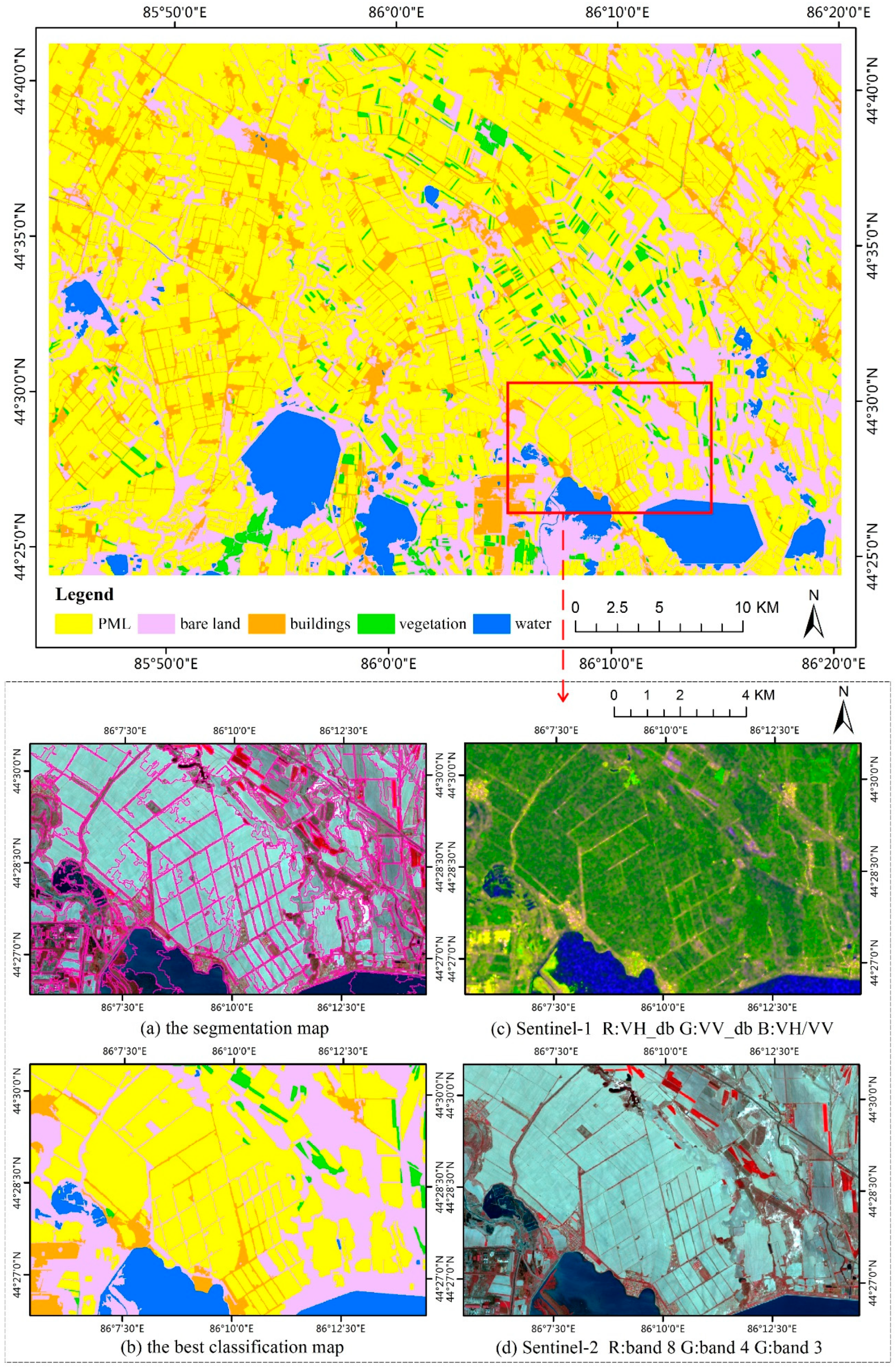
The different strategies produced different classification results. Of all the classification tests, SVM and RF classifiers performed much better than the CART classifier. Using spectral, index and textural features on integrated S1 and S2 data with the SVM classifier had the best classification accuracy of 94.34%, which is shown in Figure 6.

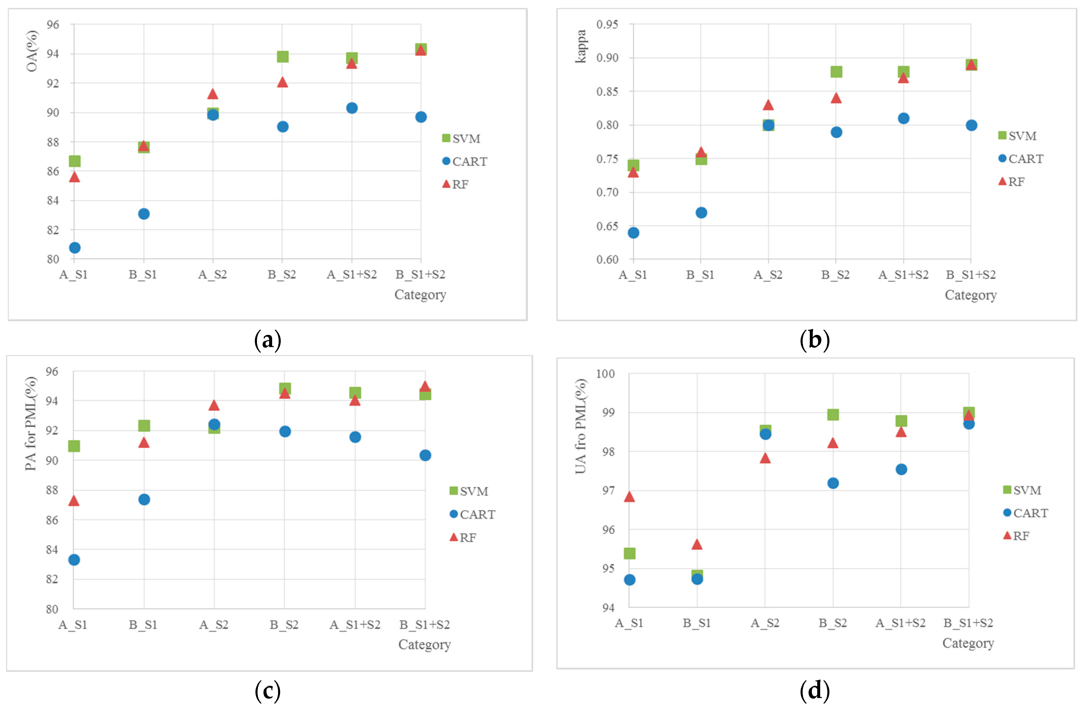
The scatterplots comparing the accuracy assessment results (i.e., OA, Kappa coefficient, PA for PML class and UA for PML class) of different classifications are presented in Figure 7. On SVM and RF classifiers, textural information played a positive role in classifying PML with 1–3% increase in terms of both overall accuracy and producer’s accuracy for PML. However, the CART classifier turned out to be less positive to textural information using S2 or integrated S1 and S2 data. Maybe it was because of the limitation, which a single tree CART classifier produced and high-dimension textural features held. When using S1 alone, textural information improved the classification accuracy regardless of the classification algorithms.

Regarding the classification results using SAR images alone, it turned out that based on the S1-and-S2 segmentation, S1 showed favorable results with an overall accuracy of around 85%. Sometimes, the producer’s accuracy for PML could exceed 90% on S1 alone. The best overall classification accuracy using S1 alone was 87.72% with the RF classifier. The object-based classification method we proposed greatly improved the classification performance by using SAR images alone, which could provide new insights into microwave remote sensing classification.

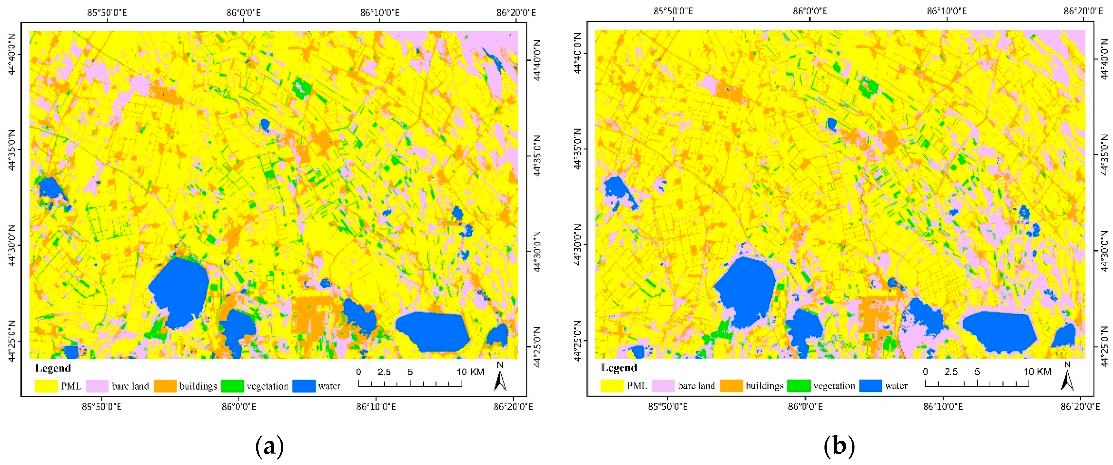
Conducting PML classification on S2 images alone already presented good classification results with an overall accuracy around 90% and kappa coefficient around 0.85. A comparison of the best object-based PML classifications using S1 alone and S2 alone is shown in Figure 8. Adding S1 images to S2 images could improve the overall accuracy by 1–3%. The improvement was more obvious on RF and SVM classifiers.

4.3. Importance of Features Used in PML Classification

According to the CART classifier, the rankings of 10 of the most important features using spectral, index, and textural information on S1, S2, and integrated S1-and-S2 data for PML classification are depicted in

Table 4. Feature importance in CART using different band combinations. (SD: Standard deviation).

S1 and S2		S1		S2
Features	Importance	Features	Importance	Features	Importance
Mean band 1	0.13	Mean VH_db	0.22	NDVI	0.11
Mean band 8	0.10	Mean VH/VV	0.14	Mean band 8	0.11
NDVI	0.10	Mean VV_db	0.11	GLCM-d	0.10
SD band 2	0.09	SD VV_db	0.09	Mean band 1	0.09
SD VV_db	0.09	GLCM-e-VV_db	0.08	SD band 3	0.09
GLCM-d	0.08	GLCM-h-VV_db	0.07	Mean band 3	0.08
Mean band 3	0.07	GLCM-c-VH_db	0.07	GLCM-c-8	0.06
Mean VH/VV	0.07	GLCM-d-VH_db	0.05	SD band 12	0.05
SD band 5	0.06	GLCM-e-VH/VV	0.05	PMLI	0.05
Mean band 4	0.04	SD VH_db	0.04	GLCM-h	0.05

.

In S2, the mean values of band 8 and band 1 of S2 and NDVI were very important in building the regression tree, while the textural information played a minor role. In S1, the mean values of VH_db, VV_db, and VH/VV were the most important in classifying PML. The importance of textural features were also indicated. It is worth noting that VH/VV were very helpful in PML extraction.

5. Discussion

The quality of segmentation results has the following impact on the quality of object-based classification. The ESP2 tool presents a good way to choose the optimal scale parameter of MRS automatically. The ED2 index can measure the segmentation performance and assist in the selection of segmentation strategies. For S2 data, four original 10 m-resolution bands had the best segmentation result based on ESP2 and ED2. Its effectiveness has also been investigated by Novelli et al. [15]. Using S1 images alone for segmentation was not a wise decision since it showed unsatisfactory results, but further research is needed on this issue. Carrying out segmentation on fused S1 and S2 data was a novel idea and it turned out to be better than using S1 or S2 alone.

The textural features derived from Haralick’s matrices had improved the classification accuracy to some extent. It was especially true for implementing classification on SAR images because they carried useful textural information. Textural features played a minor positive role in classifying PML by using integrated S1 and S2 data. However, MDI certainly did not play a very positive role in PML classification as previous studies stated [14].

Figure 7 showed that the classification accuracy was improved by adding SAR data into optical data, especially on SVM and RF classifiers. Microwave remote sensing images could help PML classification. Further research could be explored regarding the combined use of S1 and S2.

It was important to highlight that the OBIA approach we proposed could improve the classification performance greatly in SAR images alone with the best overall accuracy of 87.72%. Previous work showed an overall accuracy of nearly 75% of pixel-based classification in SAR remote sensing data [21]. Since the ground objects do not change very rapidly and SAR images are not impacted by cloud and weather, based on the segmentation of one scene of SAR and optical images at a certain date it is possible to detect PML changes over a certain period using SAR images alone.

As for the three machine learning algorithms, SVM and RF classifiers performed much better than CART. SVM and RF classifiers produced similar classification results and the classification accuracies of SVM were slightly higher than those of RF most of the time. Using spectral, index and textural features from fused S1 and S2 data with SVM produced the best classification results. However, all the classifiers tended to confuse and misclassify bare land and buildings. This occurred because the ground presented mixed characteristics in bare land and buildings and the earthen rows were likely to be segmented with bare land or buildings into one object. However. despite the confusion between bare land and buildings in classification, PML was not misclassified. Another misclassification lay in the intersected area of PML, bare land, and vegetation where land cover changes in different seasons.

Although the CART classifier had the lowest classification accuracy among the three, the feature importance table it generated could provide some useful information in improving the classification process. Choosing 15–20 important features, CART suggested instead of all mentioned features for classification, RF and SVM could produce slightly better classification results.

By integrating S1 with S2, 15 bands of the dataset were created, which hindered the segmentation and classification process. We thought it would be a good idea to reduce the dimensions by the principal component analysis. However it turned out the overall classification accuracy would decrease a bit after performing the dimension reduction. Therefore, all bands were used in generating the final PML map.

6. Conclusions

In this study, a new object-based approach with three machine learning algorithms was proposed to map PML with optical data, SAR data, and a combination of the two. This was the first study on object-based PML classification using S1 and S2 images. We also compared classification results regarding whether or not to use textural features.

The first stage of the OBIA was to obtain an optimal segmentation for PML extraction by MRS based on the ESP2 tool by, taking both optical and SAR data into consideration. Based on the evaluation of ED2 using 240 PML reference polygons, we found that the combination of four original 10 m-resolution S2 bands and two S1 bands produced the best segmentation result.

On the basis of the best segmentation, different classification strategies, which consisted of using S1 data, S2 data, or both, selecting spectral, backscattering, index, and textural features and carrying out CART, RF, and SVM classifiers, were implemented. The classification accuracy assessment indicated that the best classification result was achieved by using spectral, index, and textural information from integrated S1 and S2 data with the SVM classifier.

Among the three machine learning algorithms, RF and SVM classifiers performed way better than CART. The two classifiers yielded similar classification results while SVM was slightly better in some cases. Textural information helped improve the overall classification accuracy by 1–3% with SVM and RF classifiers. However it did not show such benefits in classifying PML with a CART classifier. Adding S1 data to S2 data could also improve the classification performance with a 1–3% increase of overall accuracy. S1 SAR images were proven to play a positive role in classifying PML due to its unique backscatter information. The OBIA method we developed was able to improve the PML classification accuracy by using S1 data alone and, achieving a best overall accuracy of 87.72% with the RF classifier. According to the feature importance obtained from the CART classifier, the mean values of band 8, band 1, and NDVI were very important in building the regression tree when S2 data was included. VH/VV band and textural features derived from S1 were very helpful in PML extraction.

This study investigated the OBIA method by using the combination of S1 and S2 data in PML classification and yielded satisfactory results. The potential of the combined use of S1 and S2 in PML and other land cover classification should be explored further.

References

- Takakura, T.; Wei, F. Introduction. In Climate under Cover-Digital Dynamic Simulation in Plant Bio-Engineering, 2nd ed.; Kluwer Academic Publishers: Dordrecht, The Netherlands, 2002; Volume 1, pp. 1–6. [Google Scholar]
- Lu, L.Z.; Di, L.P.; Ye, Y.M. A Decision-Tree Classifier for Extracting Transparent Plastic-Mulched Landcover from Landsat-5 TM Images. IEEE J. Sel. Top. Appl. Earth Obs. Remote Sens. 2014, 7, 4548–4558. [Google Scholar] [CrossRef]
- Lu, L.Z.; Hang, D.W.; Di, L.P. Threshold model for detecting transparent plastic-mulched landcover using moderate-resolution imaging spectroradiometer time series data: A case study in southern Xinjiang, China. J. Appl. Remote Sens. 2015, 9, 097094. [Google Scholar] [CrossRef]
- Zhou, D.G. Analysis of situations of China agro-film industry (2010) and countermeasures for its development. China Plast. 2010, 24, 9–12. [Google Scholar]
- Agüera, F.; Aguilar, F.J.; Aguilar, M.A. Using texture analysis to improve per-pixel classification of very high resolution images for mapping plastic greenhouses. ISPRS-J. Photogramm. Remote Sens. 2008, 63, 635–646. [Google Scholar] [CrossRef]
- Koc-San, D. Evaluation of different classification techniques for the detection of glass and plastic greenhouses from WorldView-2 satellite imagery. J. Appl. Remote Sens. 2013, 7, 073553. [Google Scholar] [CrossRef]
- Novelli, A.; Tarantino, E. Combining ad hoc spectral indices based on LANDSAT-8 OLI/TIRS sensor data for the detection of plastic cover vineyard. Remote Sens. Lett. 2015, 6, 933–941. [Google Scholar] [CrossRef]
- Chen, Z.; Wang, L.; Wu, W.; Jiang, Z.; Li, H. Monitoring Plastic-Mulched Farmland by Landsat-8 OLI Imagery Using Spectral and Textural Features. Remote Sens. 2016, 8, 353. [Google Scholar]
- Chen, Z. Mapping Plastic-Mulched Farmland with Multi-Temporal Landsat-8 Data. Remote Sens. 2017, 9, 557. [Google Scholar]
- Chen, Z.; Wang, L.; Liu, J. Selecting Appropriate Spatial Scale for Mapping Plastic-Mulched Farmland with Satellite Remote Sensing Imagery. Remote Sens. 2017, 9, 265. [Google Scholar]
- Tarantino, E.; Figorito, B. Mapping Rural Areas with Widespread Plastic Covered Vineyards Using True Color Aerial Data. Remote Sens. 2012, 4, 1913–1928. [Google Scholar] [CrossRef]
- Lu, L.Z.; Huang, Y.L.; Di, L.P.; Hang, D.W. Large-scale subpixel mapping of landcover from MODIS imagery using the improved spatial attraction model. J. Appl. Remote Sens. 2018, 12, 046017. [Google Scholar] [CrossRef]
- Aguilar, M.; Bianconi, F.; Aguilar, F.; Fernández, I. Object-Based Greenhouse Classification from GeoEye-1 and WorldView-2 Stereo Imagery. Remote Sens. 2014, 6, 3554–3582. [Google Scholar] [CrossRef]
- Aguilar, M.; Nemmaoui, A.; Novelli, A.; Aguilar, F.; García Lorca, A. Object-Based Greenhouse Mapping Using Very High Resolution Satellite Data and Landsat 8 Time Series. Remote Sens. 2016, 8, 513. [Google Scholar] [CrossRef]
- Novelli, A.; Aguilar, M.A.; Nemmaoui, A.; Aguilar, F.J.; Tarantino, E. Performance evaluation of object based greenhouse detection from Sentinel-2 MSI and Landsat 8 OLI data: A case study from Almería (Spain). Int. J. Appl. Earth Obs. 2016, 52, 403–411. [Google Scholar] [CrossRef]
- Aguilar, M.; Aguilar, F.; García Lorca, A.; Guirado, E.; Betlej, M.; Cichon, P.; Nemmaoui, A.; Vallario, A.; Parente, C. Assessment of multiresolution segmentation for extracting greenhouses from WorldView-2 imagery. Int. Arch. Photogramm. Remote Sens. Spat. Inf. Sci. 2016, XLI-B7, 145–152. [Google Scholar] [CrossRef]
- Aguilar, M.A.; Vallario, A.; Aguilar, F.J.; Lorca, A.G.; Parente, C. Object-based greenhouse horticultural crop identification from multi-temporal satellite imagery: A case study in Almeria, Spain. Remote Sens. 2015, 7, 7378–7401. [Google Scholar] [CrossRef]
- Wu, C.F.; Deng, J.S.; Wang, K.; Ma, L.G.; Tahmassebi, A.R.S. Object-based classification approach for greenhouse mapping using Landsat-8 imagery. Int. J. Agric. Biol. Eng. 2016, 9, 79–88. [Google Scholar]
- McNairn, H.; Champagne, C.; Shang, J.; Holmstrom, D.; Reichert, G. Integration of optical and Synthetic Aperture Radar (SAR) imagery for delivering operational annual crop inventories. ISPRS-J. Photogramm. Remote Sens. 2009, 64, 434–449. [Google Scholar] [CrossRef]
- Veloso, A.; Mermoz, S.; Bouvet, A.; Toan, T.L.; Planells, M.; Dejoux, J.F.; Ceschia, E. Understanding the temporal behavior of crops using sentinel-1 and sentinel-2-like data for agricultural applications. Remote Sens. Environ. 2017, 199, 415–426. [Google Scholar] [CrossRef]
- Chen, Z.; Li, F. Mapping Plastic-Mulched Farmland with C-Band Full Polarization SAR Remote Sensing Data. Remote Sens. 2017, 9, 1264. [Google Scholar]
- Sentinel-1 Product Definition. Available online: https://sentinel.esa.int/documents/247904/1877131/Sentinel-1-Product-Definition (accessed on 28 June 2018).
- Lee, J.S.; Grunes, M.R.; Grandi, G.D. Polarimetric SAR speckle filtering and its implication for classification. IEEE Trans. Geosci. Remote Sens. 1999, 37, 2363–2373. [Google Scholar]
- Small, D.; Schubert, A. Guide to ASAR Geocoding; RSL-ASAR-GC-AD; The University of Zurich: Zürich, Switzerland, March 2008. [Google Scholar]
- Muller-Wilm, U.; Louis, J.; Richter, R.; Gascon, F.; Niezette, M. Sentinel-2 Level 2A Prototype Processor: Architecture, Algorithms and First Results. In Proceedings of the ESA Living Planet Symposium, Edinburgh, UK, 9–13 September 2013. [Google Scholar]
- The Sentinel Application Platform (SNAP). Available online: http://step.esa.int/main/download (accessed on 28 June 2018).
- Baatz, M.; Schape, A. Multiresolution Segmentation: An Optimization Approach for High Quality Multi-Scale Image Segmentation. In Angewandte Geographische Informations-Verarbeitung XII; Strobl, J., Blaschke, T., Eds.; Wichmann Verlag: Karlsruhe, Germany, 2000; pp. 12–23. [Google Scholar]
- Benz, U.C.; Hofmann, P.; Willhauck, G.; Lingenfelder, I.; Heynen, M. Multi-resolution, object-oriented fuzzy analysis of remote sensing data for GIS-ready information. ISPRS-J. Photogramm. Remote Sens. 2004, 58, 239–258. [Google Scholar] [CrossRef]
- Tian, J.; Chen, D.M. Optimization in multi-scale segmentation of high-resolution satellite images for artificial feature recognition. Int. J. Remote Sens. 2007, 28, 4625–4644. [Google Scholar] [CrossRef]
- Dragut, L.; Tiede, D.; Levick, S.R. ESP: A tool to estimate scale parameters for multiresolution image segmentation of remotely sensed data. Int. J. Geogr. Inf. Sci. 2010, 24, 859–871. [Google Scholar] [CrossRef]
- Dragut, L.; Eisank, C. Automated object-based classification of topography from SRTM data. Geomorphology 2012, 141, 21–33. [Google Scholar] [CrossRef] [PubMed]
- Dragut, L.; Csillik, O.; Eisank, C.; Tiede, D. Automated parameterisation for multi-scale image segmentation on multiple layers. ISPRS-J. Photogramm. Remote Sens. 2014, 88, 119–127. [Google Scholar] [CrossRef] [PubMed]
- Liu, Y.; Bian, L.; Meng, Y.; Wang, H.; Zhang, S.; Yang, Y.; Shao, X.; Wang, B. Discrepancy measures for selecting optimal combination of parameter values in object-based image analysis. ISPRS-J. Photogramm. Remote Sens. 2012, 68, 144–156. [Google Scholar] [CrossRef]
- Novelli, A.; Aguilar, M.A.; Aguilar, F.J.; Nemmaoui, A.; Tarantino, E. AssesSeg—A Command Line Tool to Quantify Image Segmentation Quality: A Test Carried Out in Southern Spain from Satellite Imagery. Remote Sens. 2017, 9, 40. [Google Scholar] [CrossRef]
- Clinton, N.; Holt, A.; Scarborough, J.; Yan, L.; Gong, P. Accuracy assessment measures for object-based image segmentation goodness. Photogramm. Eng. Remote Sens. 2010, 76, 289–299. [Google Scholar] [CrossRef]
- Novelli, A.; Aguilar, M.A.; Aguilar, F.J.; Nemmaoui, A.; Tarantino, E. C_AssesSeg Concurrent Computing Version of AssesSeg: A Benchmark between the New and Previous Version. In Computational Science and Its Applications—ICCSA 2017, Proceedings of the International Conference on Computational Science and Its Applications, Trieste, Italy, 3–6 July 2017; Springer: Cham, Switzerland, 2017. [Google Scholar]
- Trimble Germany GmbH. eCognition Developer 9.0.1 Reference Book; Trimble Germany GmbH: Munich, Germany, 2014. [Google Scholar]
- Rouse, J.W.; Haas, R.H.; Schell, J.A.; Deering, D.W. Monitoring vegetation systems in the great plains with ERTS. In Proceedings of the Third ERTS Symposium, NASA SP-351, Washington, DC, USA, 10–14 December 1973. [Google Scholar]
- Salas, E.A.L.; Henebry, G.M. Separability of maize and soybean in the spectral regions of chlorophyll and carotenoids using the moment distance index. Isr. J. Plant Sci. 2012, 60, 65–76. [Google Scholar] [CrossRef]
- Salas, E.A.L.; Boykin, K.G.; Valdez, R. Multispectral and texture feature application in image-object analysis of summer vegetation in Eastern Tajikistan Pamirs. Remote Sens. 2016, 8, 78. [Google Scholar] [CrossRef]
- Haralick, R.M.; Shanmugam, K.; Dinstein, I.H. Textural features for image classification. IEEE Trans. Syst. Man Cybern. 1973, 3, 610–621. [Google Scholar] [CrossRef]
- Kaszta, Z.; Kerchove, R.V.D.; Ramoelo, A.; Cho, M.A.; Madonsela, S.; Mathieu, R.; Wolff, E. Seasonal Separation of African Savanna Components Using Worldview-2 Imagery: A Comparison of Pixel- and Object-Based Approaches and Selected Classification Algorithms. Remote Sens. 2016, 8, 763. [Google Scholar] [CrossRef]
- Jing, W.; Yang, Y.; Yue, X.; Zhao, X. Mapping Urban Areas with Integration of DMSP/OLS Nighttime Light and MODIS Data Using Machine Learning Techniques. Remote Sens. 2015, 7, 12419–12439. [Google Scholar] [CrossRef]
- Breiman, L.; Friedman, J.H.; Olshen, R.A.; Stone, C.J. Classification and Regression Trees; Wadsworth & Brooks: Monterey, CA, USA, 1984; ISBN 9781351460491. [Google Scholar]
- Qian, Y.; Zhou, W.; Yan, J.; Li, W.; Han, L. Comparing Machine Learning Classifiers for Object-Based Land Cover Classification Using Very High Resolution Imagery. Remote Sens. 2014, 7, 153–168. [Google Scholar] [CrossRef]
- Breiman, L. Random forests. Mach. Learn. 2001, 45, 5–32. [Google Scholar] [CrossRef]
- Rodriguez-Galiano, V.F.; Ghimire, B.; Rogan, J.; Chica-Olmo, M.; Rigol-Sanchez, J.P. An assessment of the effectiveness of a random forest classifier for land-cover classification. ISPRS-J. Photogramm. Remote Sens. 2012, 67, 93–104. [Google Scholar] [CrossRef]
- Gislason, P.O.; Benediktsson, J.A.; Sveinsson, J.R. Random Forests for Land Cover Classification. Pattern Recognit. Lett. 2006, 27, 294–300. [Google Scholar] [CrossRef]
- Cortes, C.; Vapnik, V. Support-Vector Networks. Mach. Learn. 1995, 20, 273–297. [Google Scholar] [CrossRef]
- Congalton, R.G. A review of assessing the accuracy of classifications of remotely sensed data. Remote Sens. Environ. 1991, 37, 35–46. [Google Scholar] [CrossRef]
- Wang, X.; Liu, S.; Du, P.; Liang, H.; Xia, J.; Li, Y. Object-based change detection in urban areas from high spatial resolution images based on multiple features and ensemble learning. Remote Sens. 2018, 10, 276. [Google Scholar] [CrossRef]
Figure 1.
The study area in northern Xinjiang, China. Coordinate System: WGS_1984_UTM_zone_45N. Sentinel-2 false color image: R: band 8; G: band 4; B: band 3.
Figure 2.
Plastic-mulched landcover presences in the study area. (a–d): some photos of PML in Shihezi, Xinjiang, China.
Figure 3.
The spectrum and backscattering information from Sentinel-1 and Sentinel-2 with different plastic-mulched landcover (PML). (a) The spectrum view from Sentinel-2; (b) The backscattering view from Sentinel-1.
Figure 4.
The workflow of the study.
Figure 5.
The best segmentation results: using four original 10 m-resolution bands in Sentinel-2 and two bands (VH_db, VV_db) in Sentinel-1. Scale parameter: 254.
Figure 6.
The best Plastic-Mulched Landcover (PML) classification: using spectral, index, and textural features on integrated Sentinel-1 and Sentinel-2 data with the SVM classifier. In the zoomed area: (a) the best segmentation result, (b) the best PML classification, (c) Sentinel-1 false color image: R:VH_db, G: VV_db, B: VH/VV, (d) Sentinel-2 false color image: R: band 8, G: band 4, B: band 3.
Figure 7.
Accuracy assessment for different band combinations and feature selections on three machine learning algorithms: (a) Overall accuracy, (b) Kappa coefficient, (c) Producer’s accuracy for Plastic-Mulched Landcover (PML), and (d) User’s accuracy for PML. In the category, A_S1 means using spectral features on Sentinel-1, B_S1 means using spectral and textural features on Sentinel-1. A_S2 means using spectral and index features on Sentinel-2. B_S2 means using spectral, index, and textural features on Sentinel-2; A_S1+S2 means using spectral and index features on Sentinel-1 and Sentinel-2. B_S1+S2 means using spectral, index and textural features on Sentinel-1 and Sentinel-2.
Figure 8.
Comparison between the best object-based Plastic-Mulched Landcover (PML) classifications using Sentinel-1 and Sentinel-2: (a) object-based Sentinel-1 classification with RF classifier (b) object-based Sentinel-2 classification with the SVM classifier.