Time-Series Modeling and LLM-Based Agents for Peak Energy Management in Smart Campus Environments

Abstract

A Smart campus increasingly operates on the basis of data-driven operations, but an increasing demand for energy puts their control over costs and sustainability at risk. This study addresses the challenge of anticipating and managing energy consumption peaks in multi-campus environments by proposing a hybrid framework that combines advanced time-series forecasting models with a large language model (LLM)-driven multi-agent system. Based on the UNICON dataset, LSTM, CNN, GRU, and a combination architecture are trained and compared in terms of MAE and RMSE. The hybrid configuration achieves the greatest forecasting results by returning the minimum loss values. For the identification of critical periods, we employed a strategy based on median thresholding, which offers a categorization into low, normal, and extreme category, allowing the targeting of peak mitigation actions. We also introduce a multi-agent system based on the LLM, including the data aggregator, the forecaster, and the policy advisor, which create actionable policies informed by context. We also compare LLMs (Qwen-2.5, Gemma-2, Phi-4, Mistral, Llama-3.3) in terms of context accuracy, response relevance, semantic similarity, and retrieval/recall accuracy and fidelity, with Llama-3.3 achieving the best overall results. This framework has shown great potential, not only for energy consumption forecasting but also for developing precise policies on how to effectively manage energy consumption peaks.

1. Introduction

The smart campus concept has been developed from the foundations of the smart city concept, offering an integration of efficient, sustainable, and easy-to-use learning opportunities through the application of state-of-the-art technologies [1]. In general, a smart campus uses Internet of Things (IoT) technology, big data analytics, and artificial intelligence (AI) to produce knowledge-informed decisions based on a number of campus operations, such as energy consumption, resource management, and human demands [2]. Energy management is one area that raises a very acute subject of concern among universities all over the world as far as their use of energy comes with high financial costs. University campuses, due to large building stocks as well as the wide variety of activities undertaken within them, use great quantities of energy to maintain their activity. Colleges and universities in the United States alone consume energy valued at about USD 14 billion a year; this high energy demand not only increases the operating costs, but also contributes to the production of greenhouse gases, for which institutions need to consider efficiency and sustainability [3]. In order to deal with these problems, smart campus energy management systems use the power of smart sensors and monitoring and controlling technologies. Sustainable smart campus initiatives rely on low-power, autonomous sensor networks. Recent surveys highlight that integrating ultra-low-power design with micro-energy harvesting can make IoT nodes self-sufficient [4], reducing maintenance and enabling long-term deployments. These systems often have smart meters so that electricity, gas, and water expenditures are accurately monitored within a short time almost anywhere on the campus.

Future developments in smart campus environments include the use of Internet of Things (IoT) sensor networks to track other energy consumption determinants, such as occupancy levels, ambient temperature, humidity, and lighting levels [5]. Simultaneously, the use of analytics, especially those focused on big data methods and machine learning algorithms, can ease the analysis of usage patterns, the identification of energy consumption inefficiencies, and the prediction of future demand patterns [6]. Intelligent building management systems are examples of automated control architecture used to regulate heating, ventilation, air conditioning, lighting, and other high-energy-consumption subsystems based on real-time data streams, to maximize energy use according to current operational needs [7]. Many facilities are also incorporating renewable generation resources, such as photovoltaic panels and wind turbines, to supplement traditional energy sources and support sustainability goals [8].

To enhance the capabilities of these systems, multi-agent networks based on large language models (LLMs) were introduced. The autonomous agents that are driven by LLMs operate to assist with various aspects of energy control, providing a more adaptable and responsive management method. An example here, in a smart campus energy-management setting, is a multi-agent framework based on LLM, which comprises multiple interconnected agents; each agent has an LLM, reads complex data, coordinates its actions, issues detailed reports, and provides specific advice on energy optimization [9]. This LLM-based multi-agent system can meet the challenges of a data-rich campus environment by providing contextual and adaptive solutions that go beyond the capabilities of traditional single-agent or rule-based systems. The integration of LLM-based multi-agent systems into smart campuses represents a significant advance in AI, leveraging the capabilities of natural language to interact intuitively and operate dynamically in complex environments. These systems enable institutions to achieve greater degrees of efficiency and sustainability and, at the same time, increase user comfort, thus creating a new standard of responsive, data-driven decision-making in the management of campus resources and infrastructure. This area of research is probably receiving particular attention both scientifically and practically, as smart campus initiatives offer the potential to achieve significant energy savings and improve the sustainability of future higher education infrastructures. This paper presents a hybrid framework that combines advanced time series models and agent-based systems powered by large language models (LLMs) to address the challenge of efficient energy management in smart campuses. Employing models such as LSTM, GRU, and a hybrid architecture, the framework accurately predicts energy consumption, with the hybrid model achieving the highest accuracy. Using a median-based threshold, peak energy periods are identified, and an LLM-driven agent-based system generates adaptive energy policies to optimize operations and improve sustainability. This paper begins by reviewing related work and methodologies; then, it explains the hybrid framework and its implementation. The performance of the framework is demonstrated by a detailed case study using the UNICON dataset, which includes time series energy consumption data from a multi-campus university. This case study highlights the system’s ability to predict demand, classify peaks, and provide actionable policy recommendations for dynamic energy management.

This paper is organized as follows. Section 2 reviews related work on energy forecasting, peak detection, and intelligent energy management systems in smart campus environments. Section 3 presents the proposed hybrid framework, detailing the data preprocessing steps, the time-series forecasting models, and the median-based peak detection strategy. Section 4 evaluates the performance of the forecasting models across multiple campuses using error metrics. Section 5 describes the energy peak classification methodology and its integration into the decision-making process. Section 6 introduces the LLM-based multi-agent system and the retrieval-augmented generation pipeline for policy recommendation, along with the adopted evaluation metrics. Section 7 discusses the experimental results and comparative analysis of the tested models. Finally, Section 8 concludes the paper and outlines limitations and future research directions.

2. Literature Reviews

To achieve our goal, we used the UNICON dataset [10], derived from La Trobe University’s Energy AI/Analytics platform, which has been widely used to explore energy optimization in smart campuses. As an open dataset comprising electricity, gas, and water consumption data for over 100 buildings, it supports a variety of academic, residential, and administrative uses. Recent advances in energy management have highlighted the potential of predictive modeling and intelligent systems in optimizing energy use.

The UNICON dataset has been the focus of several studies. Sumanasena et al. in his paper [11] used UNICON to address the challenges of electric vehicle infrastructure (EVI), focusing on demand profiling, forecasting, and optimization. Their framework used artificial intelligence to efficiently manage energy consumption and charging schedules, demonstrating significant improvements in demand prediction and explicability. However, their work was primarily focused on electric vehicle infrastructure and does not address the broader challenges of energy management in smart campuses. Similarly, Moraliyage et al. [12] have used UNICON to validate energy conservation measures (ECM), using robust and explainable AI approaches. Their framework combines pre- and post-retrofit data to assess energy savings, highlighting the role of AI in measurement and verification (M&V) protocols. While useful, this work is limited to M&V validation without addressing predictive modeling or peak energy management. With regard to energy consumption prediction, recent work by Zhang et al. has demonstrated that LSTM models, when combined with attention mechanisms and transfer learning, achieve high accuracy in short-term residential load prediction, particularly for non-linear consumption models [13]. Similarly, Son and Kim have highlighted the effectiveness of deep neural networks, including GRU and LSTM, in accurately predicting building energy consumption using real-world datasets [14]. Barbato have developed a framework for smart campuses that integrates local renewable energy sources, battery banks, and controllable loads [15]. Their system optimizes demand–response interactions through predictive energy scheduling that ensures user comfort while reducing energy expenditure. Yuliansyah et al. proposed an IoT-based energy monitoring system for a smart campus, enabling the real-time data acquisition and visualization of energy usage [16]. Their work focused on the role of monitoring in improving efficiency but did not explore predictive analytics or policy generation. Talei presented an AI-tuned microgrid system integrated with IoT sensors to optimize load balancing and renewable energy use on campuses [17]. In another work, the authors describe a smart campus case study where large language models process sensor data and user preferences to adjust room settings and network configurations, achieving energy savings of 20–30% [18].

With regard to energy peak detection problems, Wang and Sung-Hoon have proposed a real-time peak detection algorithm, suitable for load forecasting in dynamic energy environments, that adapts effectively to variations in baseline consumption [19]. M. A. Petri et al. also propose a fundamental review of anomaly detection methods, many of which are applicable to peak detection in energy consumption data [20]. Bakakeu et al. have shown that multi-agent reinforcement learning frameworks can improve the energy efficiency of cyber-physical production systems by enabling decentralized control strategies [21]. Luo extended this approach to the context of smart grids, showing that agents trained by machine learning can significantly optimize energy flows and load coordination [22].

In addition, Saleh [23] have suggested the Follow-Me AI infrastructure, which leverages LLM-based agents to simulate the behavior of users and adjust the environment to the movements and preferences of people. The AI approach proposed provides a proactive solution to energy waste mitigation and a more comfortable experience for users, which proves the potential of LLMs and generative artificial intelligence to offer effective and efficient solutions in intelligent environments. In the context of agent and LLM integration in energy systems, Xiao and Xu [24] proposed a multi-agent model of automated energy optimization, which uses unstructured data on buildings as the input and suggests improvements with the help of an LLM. Their publication points to the possibility of using agent-based systems to address complicated processes in energy. Yang [25] also demonstrated that LLMs have the ability to aid smart grids through intelligent decision-making based on the demand signals and adapting the control strategies in real time. Similarly, Buster [26] also addressed the potential of using LLMs in the planning of energy systems, with an emphasis on their ability to combine political limits and operational data into practical advice. Regarding retrieval-augmented generation (RAG) systems, we take a direction that is consistent with the RAG paradigm presented by Lewis [27], which combines knowledge retrieval with generative models to improve the factuality and context awareness of text generation. This methodology was further improved by Izacard and Grave [28], who added more efficient passage-search mechanisms to facilitate open-domain question answering. This model forms a precedent for using the usage of LLM-driven agents and thus motivates our strategy to integrate energy prediction with policy suggestions to smart campus energy peaks.

Building on these foundations, our research introduces a new approach that combines time series models to predict energy consumption and uses a statistical approach to detect energy peaks. Once these energy peaks are detected, the agent LLM-based system will be used to automatically propose energy policies to mitigate them (like load shifting to optimize power usage or adjusting energy supply resources in real time). This concept aims to use the positive properties of predictive analytics and offers a robust framework for managing energy consumption in dynamic environments.

3. Our Approach

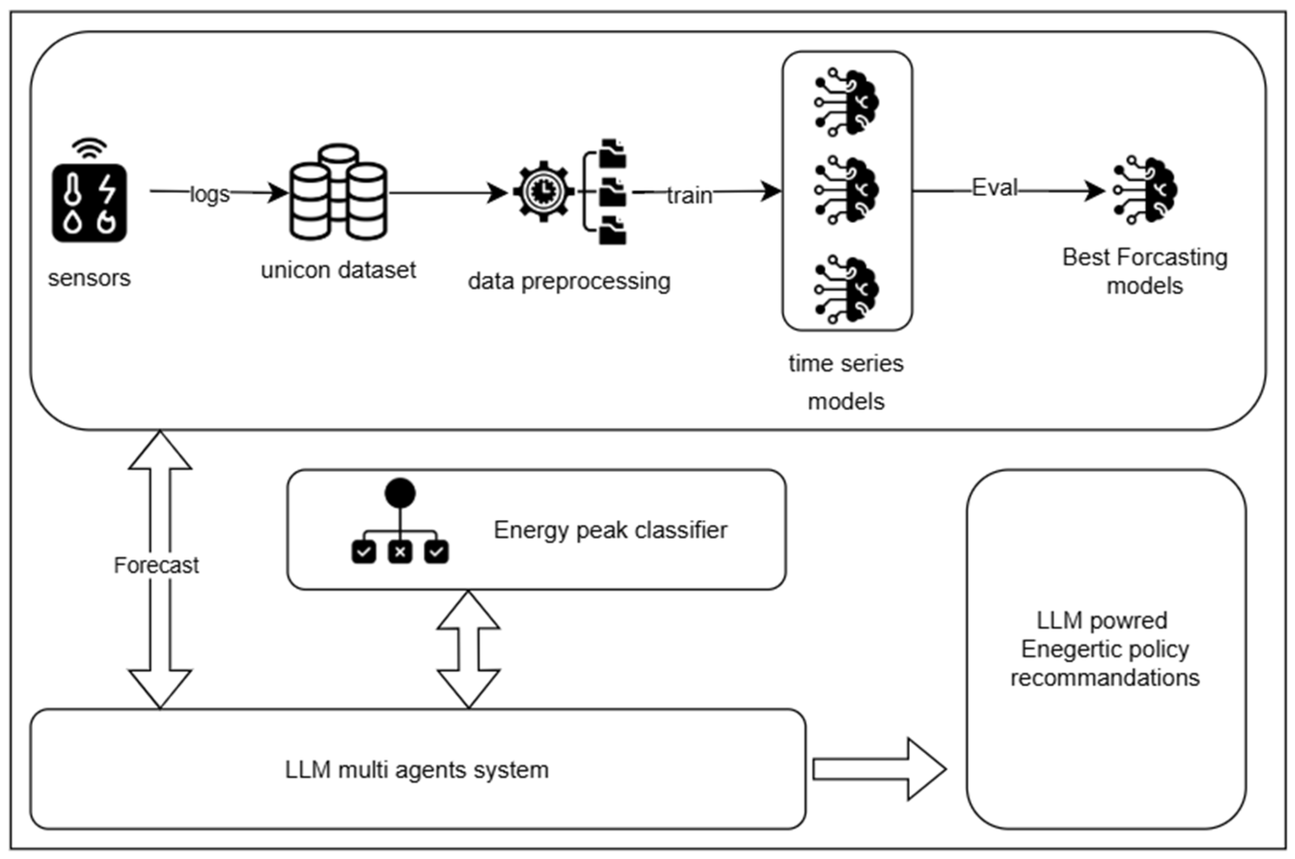
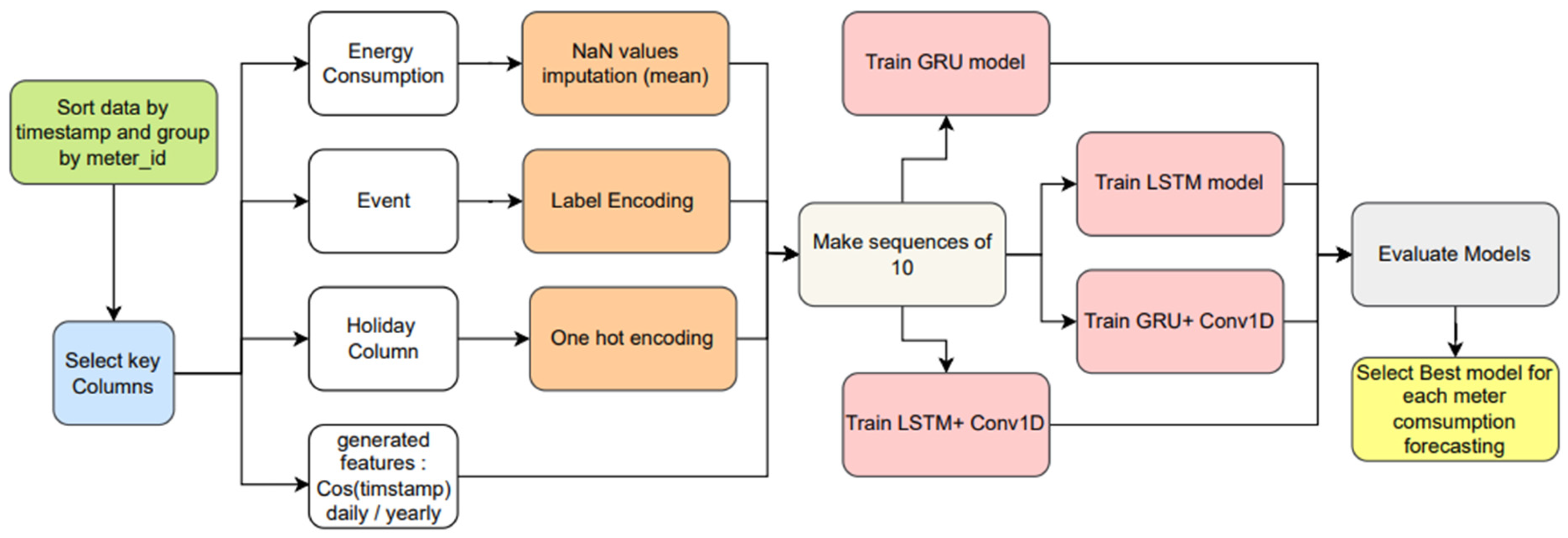
This study as shown in Figure 1 outlines the development of a framework that combines advanced machine learning models and an agent-based system utilizing large language models (LLMs) for energy consumption forecasting and energy policy recommendations in a smart campus. The main source of data was the UNICON dataset from La Trobe University. The dataset comprises detailed time-series data of electricity use in the buildings of 5 campuses, as well as meteorological variables such as temperature and humidity. For the energy prediction, we implemented and compared three state-of-the-art models: long short-term memory, which has three layers (LSTM) [29]; convolutional neural network (CNN) [30]; and a hybrid LSTM-CNN model with a gated recurrent unit (GRU) [31]. Additionally, a hybrid model that synthesizes the power of all three architectures was evaluated. Each model was trained and evaluated using Mean Absolute Error (MAE) [32] and root-mean-square error (RMSE) [32]. Peak energy demand was defined using a median-based thresholding approach, which classifies consumption values predicted for peak and non-peak times compared to the median consumption level of each electricity consumption meter. This classification allowed for the development of specific energy management strategies. To manage peak times, an LLM-based agent-based module was developed to produce policy recommendations that can be turned into actions. The LLM agents analyzed energy use patterns as well as contextual building metadata, from which adaptive measures were proposed, like the redistribution of loads, adjustments to HVAC, and integration of renewable energy. The hybrid framework was evaluated on the measurement of predictive accuracy, classification efficiency, and the quality of recommendations generated.

3.1. Dataset

The UNICON dataset [10] is an open-access dataset provided by La Trobe University’s campuses as part of its commitment to achieve net-zero carbon emissions by 2029. It represents a fundamental resource for the La Trobe Energy AI/Analytics Platform (LEAP), which is helping to monitor, predict, and optimize energy use and the management of resources by utilizing AI and data analytics. All five geographically distributed campuses were covered during a period of four years (2018–2021), including the period of the COVID-19 pandemic with its consequent drastic cuts to energy demand. UNICON has high-resolution consumption data. These include data on electricity usage at 15 min intervals, gas usage at hourly intervals, water usage at 15 min intervals, and weather data every one minute and at 10 min intervals from the nearest weather stations. Additionally, the dataset includes an annotation on key events that have occurred internally in the building, such as Energy Conservation Measures (ECMs) and Measurement and Validation activities, to support in-depth energy analysis and optimization strategies. UNICON offers detailed metadata, technical validation, and high-granularity energy usage records, making it an invaluable resource for academics, researchers, industry practitioners, sustainability experts, and policymakers. It enables the development and evaluation of AI-driven energy forecasting models, data-driven energy management policies, and benchmarking standards, contributing to sustainable and intelligent campus operations.

The following steps, shown in Figure 2, are important for cleaning and preparing UNICON data for analysis using time series techniques. Firstly, all data is grouped by the meter_id field, so that similar data is brought together. Then, to maintain the chronological order of the data, the data is sorted based on timestamp. Three key columns are adopted: energy consumption as an event column, which is a set of six values; a public holiday column, which indicates whether the day is a public holiday or not; and the weather status, including temperature and humidity. The data contained in the “event” feature is first transformed into numerical data using label encoding, as it is categorical in nature, and the “is_holiday” feature has only two values; for our model, due to the periodic nature of electricity consumption in a smart campus environment, time-derived features are generated from the timestamp information. Electricity demand is known to exhibit strong daily and seasonal cycles, which are not adequately represented by raw timestamp values. To address this limitation, sinusoidal transformations, specifically cosine-based encodings, are applied to represent temporal positions within daily and yearly cycles in a continuous manner. This encoding preserves the cyclical structure of time and avoids artificial discontinuities that occur at temporal boundaries, such as midnight or the transition between calendar years. By providing the learning models with explicit information about recurring temporal patterns, these generated features enhance the ability of recurrent and convolutional architectures to capture regular consumption behaviors and seasonal trends, leading to improved forecasting performance. To deal with the problem of data sparsity, all NaN values are imputed by the column average. In addition, the MinMaxScaler is used on the energy consumption column to scale the data, normally to between 0 and 1. Next, sequences of 10 values are obtained to enter the GRU, LSTM, CNN+GRU, and CNN+LSTM time series models. Then, we split our data for each meter into 70% for training, 15% for validation, and 15% for testing. We also adopted an early stopping of 10 epochs to avoid the overfitting issue. All the models are trained on the result obtained from every meter_id, and the desired model is chosen for each electricity consumption meter based on the minimum loss values to get the maximum accurate consumption value of energy.

3.2. Time Series Models

For the time series prediction models, the pre-processed data are used to train the following models: GRU, LSTM, GRU with Conv1D, and LSTM with Conv1D, respectively. These models are expected to give the likely energy consumption for meter ID and total meters over the whole campus and university. Predictions are recalled and checked against predefined standard thresholds and updated accordingly. If predicted consumption exceeds these values, a pre-trained campus-specific language model (LLM) is used with energy consumption policies.

3.2.1. LSTM

The long-term memory network [29], commonly known as LSTM is a type of recurrent neural network that deals with the fading gradient problem by backpropagation in time. LSTM enables the creation of extended recurrent networks, which are essential for solving complex sequence problems in machine learning. Unlike traditional neurons, LSTM networks are made up of interconnected memory blocks between layers. These blocks have specialized components that give them a higher level of intelligence than conventional neurons, as well as a memory for recent sequences. 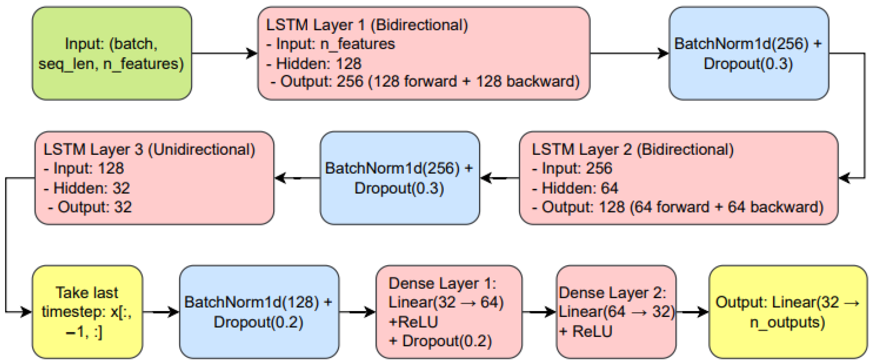In this study, the Figure 3 presents a model architecture where we employ a deep recurrent neural network composed of stacked Long Short-Term Memory (LSTM) layers. The model processes multivariate time-series inputs structured as sequences of a fixed length of 10, representing recent historical observations of campus energy usage. The architecture comprises two bidirectional LSTM (BiLSTM) layers followed by a unidirectional LSTM layer. The first BiLSTM layer uses 128 hidden units per direction, yielding a 256-dimensional output per timestep, while the second BiLSTM layer employs 64 hidden units per direction, producing 128-dimensional temporal representations. These bidirectional layers enable the model to capture short-term temporal dependencies within the observation window. Batch normalization and dropout with a rate of 0.3 are applied after each recurrent layer to stabilize training and reduce overfitting. The third LSTM layer is unidirectional, with 32 hidden units, enforcing causal temporal modeling consistent with forecasting objectives. The hidden state corresponding to the last timestep is then extracted to obtain a compact summary of the input sequence. This representation is passed to a fully connected prediction head consisting of two dense layers with ReLU activations and dropout (0.2), followed by a linear output layer that produces the final energy consumption forecast.

3.2.2. GRU

Similarly to the long short-term memory (LSTM) network, a recurrent neural network variation called Gated Recurrent Units (GRU) [31] is a recurrent neural network that uses gates to control access to information in the network. However, it has been considered relatively new as opposed to LSTMs and is an improvement in terms of its simpler architecture without a loss in performance.

Let us dive into how these gates operate. To compute the hidden state $h_t$ in a GRU, a two-step process is followed. The first thing to do will be to create a variable called the candidate hidden state:

$$h_t=\tanh \left(x_t \mathrm{\ast } U_g+\left(r_t°h_{t-1}\right) \mathrm{\ast } W_g\right)$$

(1)

In this equation, the input $x_t$ and the hidden state from the previous timestamp t − 1 are taken into account. These values are then multiplied by the reset gate output $r_t$. The whole information is then passed through a hyperbolic tangent, which produces the candidate hidden state.

Once we obtain this candidate state, this is used to develop the present hidden state at time t. This is where the update gate should help. In exercising the gates, GRUs use only one update gate and allow the historical $h_{t-1}$ value to mix with the new information that comes from the candidate state:

$$h_t=u_t°h_{t-1}+\left(1-u_t\right)°h_t$$

(2)

This equation shows how the update gate balances the previous hidden state $h_{t-1}$ with the candidate state $h_t$, determining how much each contributes to the current hidden state. In addition, this mechanism enables GRUs to successfully learn and make use of relevant information for sequential tasks.

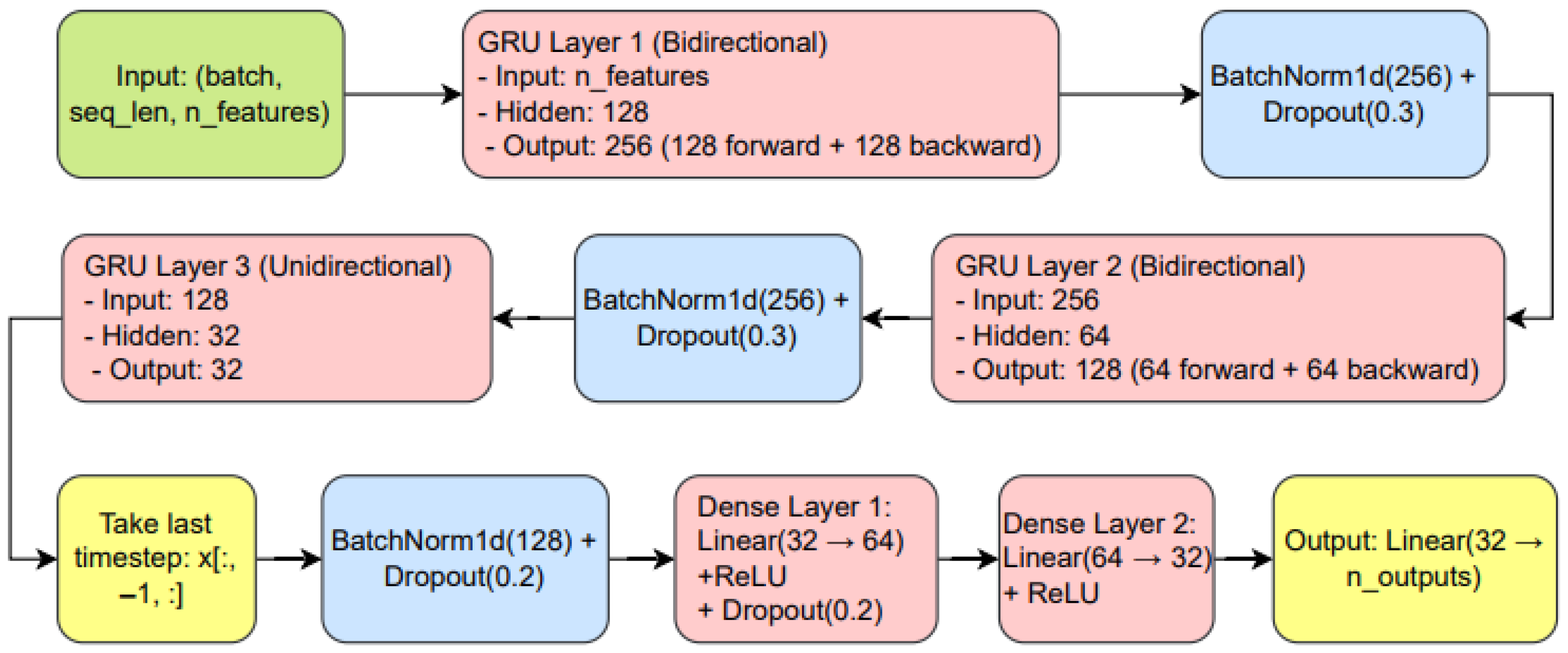
Figure 4 shows the details of the architecture of the GRU model we trained on our preprocessed data. The model processes multivariate input sequences structured as $\left(\mathrm{batch},\mathrm{seq}\_\mathrm{len},{\mathrm{n}}_{\mathrm{features}}\right)$ and is designed to capture short-term temporal dependencies within a fixed observation window. The architecture consists of three stacked GRU layers, including two bidirectional GRU layers followed by a unidirectional GRU layer. The first bidirectional GRU layer uses 128 hidden units per direction, producing a 256-dimensional representation at each timestep, while the second bidirectional GRU layer employs 64 hidden units per direction, resulting in 128-dimensional temporal features. These bidirectional layers enable the model to exploit contextual information from both forward and backward temporal directions within the input sequence. Batch normalization and dropout with a rate of 0.3 are applied after each GRU layer to improve training stability and mitigate overfitting. The final GRU layer is unidirectional, with 32 hidden units, enforcing causal temporal modeling consistent with forecasting objectives. To obtain a fixed-size representation for regression, the hidden state corresponding to the last timestep is extracted and used as a compact summary of the input sequence. This representation is then passed through a fully connected prediction head comprising two dense layers with ReLU activations and dropout (0.2), followed by a linear output layer that produces the final energy consumption forecast.

3.2.3. Conv1D

In recent academic work, convolutional neural networks (CNNs) [30] have gained a lot of attention for their outstanding performance. Thanks to convolutional calculations that are performed on the original data, CNNs can detect partial features of the data independently. Similarly, a version of CNN called Conv1D is used to convolve one-dimensional signals to find underlying relationships in sequential data. The unique feature of Conv1D is not only its capability to extract important features from sequential data, but also its ability to reduce sequence dimensionality. After being compressed to unit length, the model is suitable for regression modeling tasks. The length can also represent the number of categories, enabling the model to be used for classification tasks. The equation below represents the convolution calculation formula:

$$F\left(x\right)=\left(f \mathrm{\ast } g\right)\left(x\right)=\sum \tau =f\left(\tau \right)g\left(x-\tau \right)$$

(3)

Here, F(x) is the convolution operation between the functions f and g at position x, where f and g are functions of the corresponding arguments $\tau$ and $x-\tau$.

3.2.4. Hybrid of GRU LSTM and Conv1D

a.

CNN+GRU.

The use of convolutional neural networks (Conv1D), together with the gate recurrent unit (GRU), is a strong hybrid model for analyzing sequential data [33]. GRUs [11] are a variant of recurrent neural network architecture, which makes it easier to understand the structure of the long short-term memory (LSTM) network and which has the ability to recognize temporal dependencies. It does this mainly using two gates: the reset gate and the update gate. The gates control the flow of information and decide how much of the information from the past should be kept or forgotten. The candidate hidden state and the previous state are combined to form the hidden state of GRUs, maintaining the balance of historical information and new information. Therefore, compared with LSTM, GRUs can fully encode the sequential data with decreased computational complexity. The Conv1D layer complements GRUs by improving feature extraction from one-dimensional sequential data. Conv1D applies convolutional operations along the time axis, identifying local patterns and reducing dimensionality. This means that the model can capture complex features before feeding them through the GRU layer for temporal processing. The Conv1D layer is for extracting the same type of spatially correlated patterns (trend or periodicity) in the sequences that are very important for accurate predictions in time series tasks. The CNN+GRU hybrid model presents an advantage due to the fact that the Conv1D layer can be used to preprocess the data by extracting high-level features, followed by the fact that the GRU can be used to model temporal relationships. This combination has the potential to give a very good ratio between spatial feature extraction as well as temporal dependency modeling, making it well-suited for applications such as energy consumption forecasting.

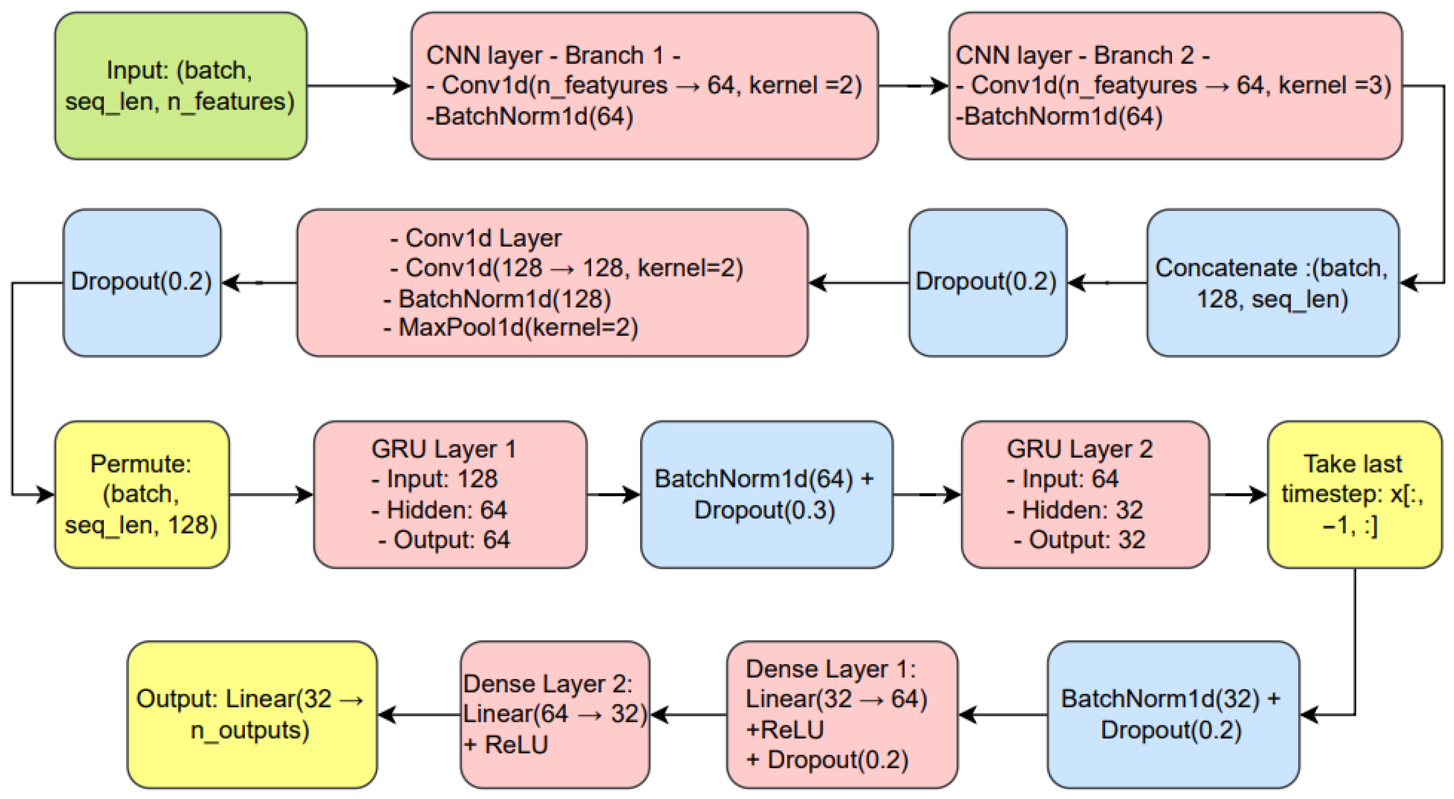
The architecture presented in Figure 5 begins with a multi-scale convolutional module composed of two parallel one-dimensional convolutional branches. The first branch applies a Conv1D layer with a kernel size of 2, while the second branch employs a kernel size of 3; both branches project the input feature space into 64 channels and are followed by batch normalization. This multi-scale design enables the extraction of temporal patterns at different resolutions, capturing both short-term variations and slightly broader temporal structures in energy consumption data. The outputs of the two convolutional branches are concatenated along the channel dimension, yielding a combined representation of size $\left(\mathrm{batch},128,\mathrm{seq}\_\mathrm{len}\right)$, followed by dropout, with a rate of 0.2 for regularization. A subsequent Conv1D layer with 128 filters and a kernel size of 2 further refines the extracted features, followed by batch normalization and max pooling to reduce temporal redundancy and emphasize salient local patterns. The resulting feature maps are then permuted to restore the temporal ordering $\left(\mathrm{batch},\mathrm{seq}\_\mathrm{len},128\right)$ and fed into a stacked GRU module. The first GRU layer employs 64 hidden units to model temporal dependencies across the convolutionally extracted features, followed by batch normalization and dropout (0.3). A second GRU layer with 32 hidden units further compresses the temporal representation while preserving sequential information relevant to forecasting. To obtain a fixed-size representation suitable for regression, the hidden state corresponding to the last timestep is extracted, providing a compact summary of the input sequence. This representation is subsequently normalized and regularized using batch normalization and dropout (0.2) and then passed through a fully connected prediction head, comprising two dense layers with ReLU activations. The final linear output layer maps the learned representation to the target space, producing the predicted energy consumption values.

b.

Conv1D+LSTM

When combined with a convolutional neural network (Conv1D), the long short-term memory (LSTM) network will form a powerful architecture that can process complex sequential data [34]. LSTMs are known for their ability to overcome the problem of gradient vanishing in recurrent neural networks. They use memory cells and specific gates (forgetting, input, and output gates) to control the flow of information in time. As a result, LSTMs are highly suitable for modeling complex temporal dynamics because they can capture long-term dependencies while paying attention to relevant features. Conv1D layers are integrated within the LSTM architecture, which will improve the process of feature extraction. These layers work by performing a convolution on the input sequences, thereby identifying local structures and patterns that are difficult to capture with purely recurrent architectures. The convolution operation reduces the dimensionality of the sequence while retaining critical information. This is then passed to the LSTM for temporal analysis. The synergy between them allows the model to first extract meaningful features from raw sequential data through convolution operations and then use the memory capabilities of the LSTM to model dependencies over time. This hybrid architecture is effective for tasks that involve both spatial and temporal complexities, like energy forecasting or time series classification, in which it is crucial to understand local patterns and long-term dependencies.

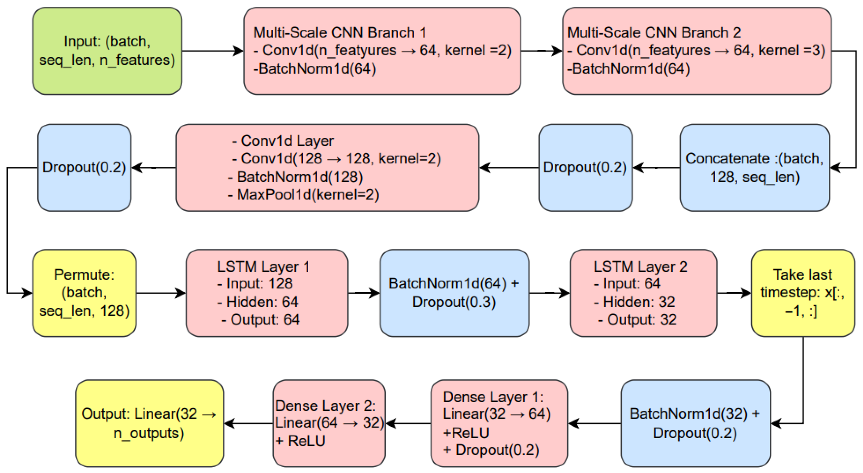
The Figure 6 presents the architecture used in our study; it begins with a multi-scale convolutional module composed of two parallel one-dimensional convolutional branches. The first branch applies to a Conv1D layer with a kernel size of 2, while the second branch uses a kernel size of 3; both branches project the input features into 64 feature maps and are followed by batch normalization. This multi-scale design enables the model to capture temporal patterns at different resolutions, improving sensitivity to both short-term fluctuations and slightly longer temporal variations in energy consumption data. The outputs of the two convolutional branches are concatenated along the channel dimension, forming a unified representation of size $\left(\mathrm{batch},128,\mathrm{seq}\_\mathrm{len}\right)$. Dropout with a rate of 0.2 is then applied for regularization. A subsequent Conv1D layer with 128 filters and kernel size 2 further refines the extracted features, followed by batch normalization and max pooling to reduce temporal redundancy and emphasize dominant local patterns. The resulting feature maps are permuted to restore a time-major format $\left(\mathrm{batch},\mathrm{seq}\_\mathrm{len},128\right)$ and passed to a stacked LSTM module. The first LSTM layer uses 64 hidden units to model temporal dependencies across the extracted convolutional features, followed by batch normalization and dropout (0.3). A second LSTM layer with 32 hidden units further compresses the temporal representation. To obtain a fixed-size vector suitable for regression, the hidden state corresponding to the last timestep is extracted, providing a compact summary of the input sequence. This representation is subsequently normalized and regularized using batch normalization and dropout (0.2) and then fed into a fully connected prediction head composed of two dense layers with ReLU activations. The final linear output layer maps the learned representation to the target space, producing the forecasted energy consumption values.

To test the performance of our deep learning models for the short-horizon electrical consumption forecasting, we used two popular methods: Mean Absolute Error (MAE) [32] and Mean Squared Error (MSE). When we deal with a nonlinear predictive model, the best way to evaluate its performance is to calculate the loss. Usually, the metrics used are the MSE (Mean Squared Error) and the MAE (mean Average Error); the MAE evaluates the absolute distance of the observations (x_i) to the predictions (y_i) on a regression, taking the average over all:

$$MSE={\displaystyle \frac{1}{n}}\sum _{i=1}^n{\left(Yi-Ŷi\right)}^2$$

(4)

$$MSE={\displaystyle \frac{1}{n}}{\sum }_{i=1}^n\left|Yi-Xi\right|={\displaystyle \frac{1}{n}}{\sum }_{i=1}^n\left|Ei\right|$$

(5)

The MSE [32] tries to calculate the average of the squared error between actual and predicted values; it is based on the L2 loss, which is a squared difference between actual and predicted values. The MSE [21] is the mean of all the L2 loss values.

4. Time Series Models Evaluation

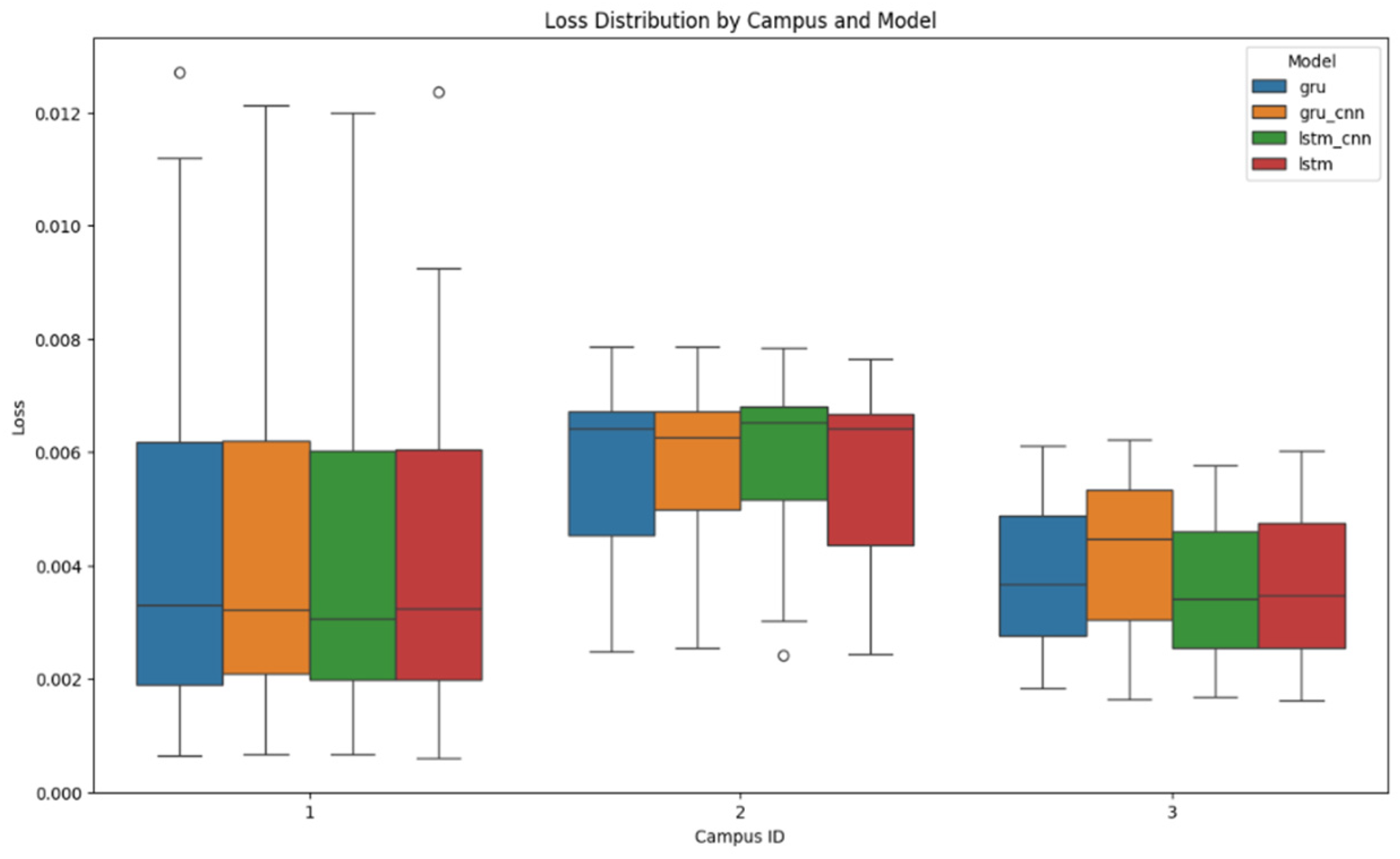
Figure 7 presents an analysis of the distribution of losses across three campuses for four different models (GRU, GRU+CNN, LSTM+CNN, and LSTM) which reveals several key insights into the performance and consistency of the models. On Campus 1, all models have relatively high median losses, with the GRU, GRU+CNN, and LSTM models showing similar median losses of around 0.003, while the LSTM+CNN model shows a slightly higher median loss of 0.006. This indicates that the models have comparable performance. There is significant variability, particularly between the GRU and GRU+CNN models, as shown by the wide interquartile ranges. For Campus 2, the GRU model shows a slightly lower median loss, just above 0.003, compared to the other models, suggesting that it handles this dataset slightly better. The GRU+CNN and LSTM+CNN models show similar performance, with median losses of around 0.004, but with a wider range for the GRU+CNN model, indicating greater variability.

In Campus 3, the GRU model performs best, with the lowest median loss of around 0.0025, followed by the GRU+CNN and LSTM models, with median losses of around 0.003. The LSTM+CNN model has the highest median loss in this campus, around 0.0035, suggesting that adding CNN layers may not significantly improve performance in this context. Overall, the GRU model tends to have a slight performance advantage, particularly in Campus 3, while the LSTM model shows more consistent performance across all campuses. The combined models show some potential but require further tuning to achieve performance levels comparable to those of the simpler GRU and LSTM models, for the isolated circular marker observed in the boxplot, it corresponds to an outlier. It represents a loss value that lies significantly outside the typical range of the data distribution of our results. These results highlight the importance of selecting and tuning models based on specific campus characteristics and also suggest that simpler models can sometimes perform better than more complex architectures.

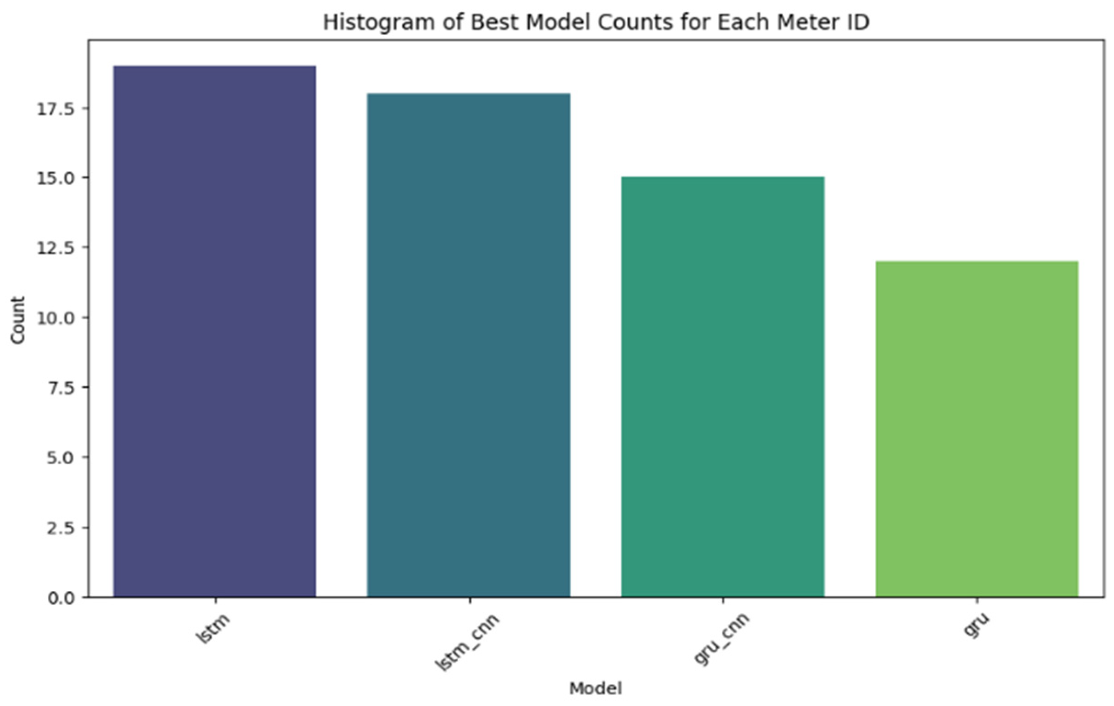
The histogram shown in Figure 8 includes an illustration of the best models for each meter ID that reveals interesting trends regarding model performance across different campuses. The LSTM model proves to be the best for around 18 m IDs, which shows the good performance of the model in capturing the temporal dependencies and accurately forecasting energy consumption. It is followed closely by the LSTM+CNN model, which combines the strength of LSTM with convolutional layers and is the best model for just under 18 m IDs. This suggests that adding CNN layers improves performance for a significant number of meter IDs. The GRU+CNN model is identified as the best for approximately 14 m IDs, demonstrating its usefulness in scenarios where the combined architecture is suited to the characteristics of the data. Finally, although the GRU model performs best for approximately 12 m IDs, it nevertheless demonstrated robustness and simplicity in specific contexts. These results highlight that the LSTM and LSTM+CNN models are generally the most effective for predicting energy consumption, while emphasizing the importance of model diversity to address the varied characteristics of data between different meter identifiers in a smart campus setting.

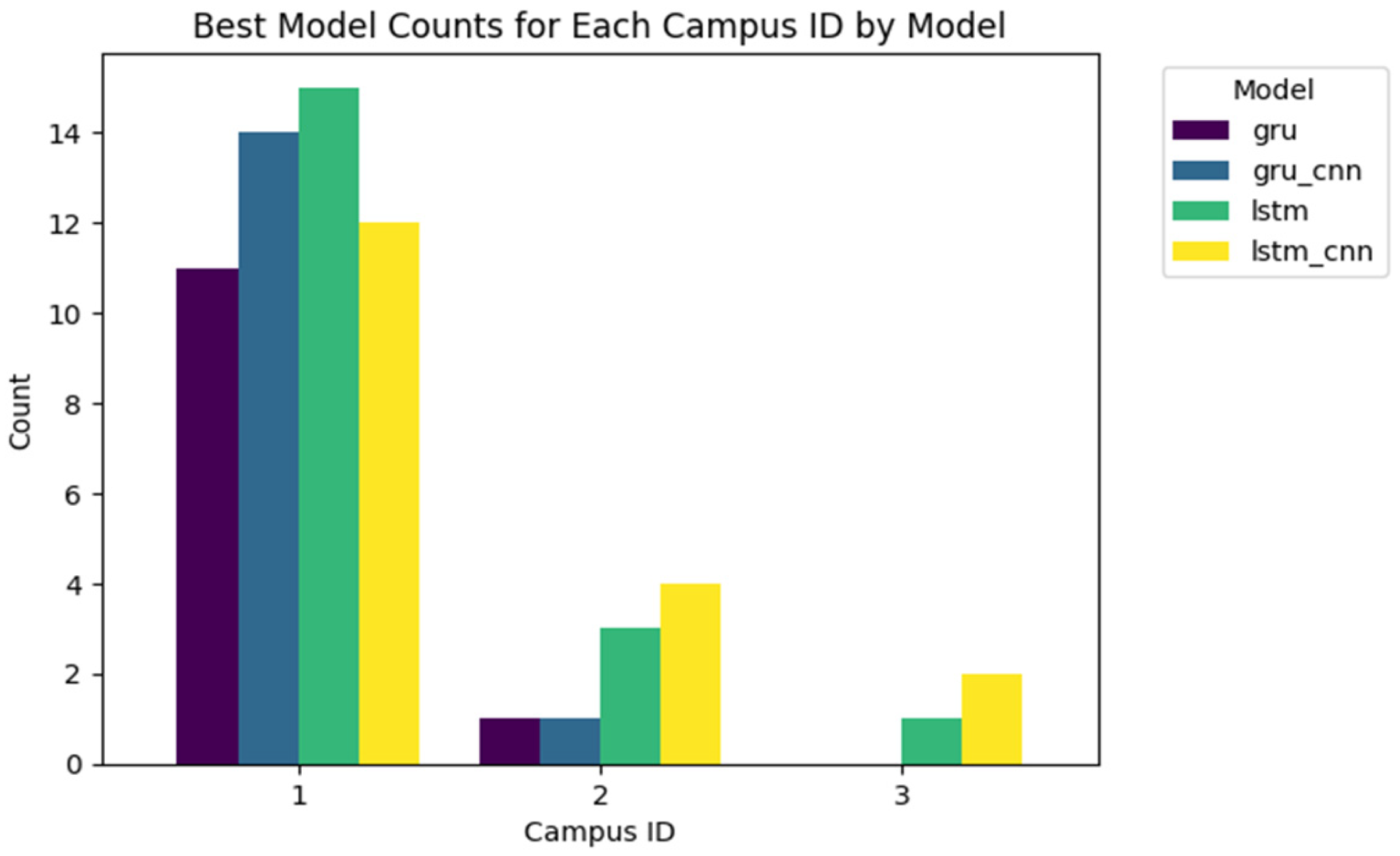
Figure 9 also shows that the LSTM and LSTM+CNN models are generally the most relevant across all campuses. For the 1st campus, the LSTM+CNN model has been remarked as the best, with around 15 m, followed by the LSTM model with 14 m and the GRU+CNN model with 13 m. In comparison, the GRU model performs fewer scores with around 11 m. On the 2nd campus, the LSTM+CNN model performs best, with 5 m, followed by the LSTM model with 4 m, the GRU+CNN model with 3 m, and the GRU model with 1 m. For the 3rd campus, the LSTM model performs best, at around 3 m, followed by the LSTM+CNN model with 2 m and the GRU+CNN model with 1 m. While LSTM-based models are efficient across different campuses, the specific characteristics of each campus influence the choice of the optimal model, highlighting the need for a best approach in predictive energy consumption modeling.

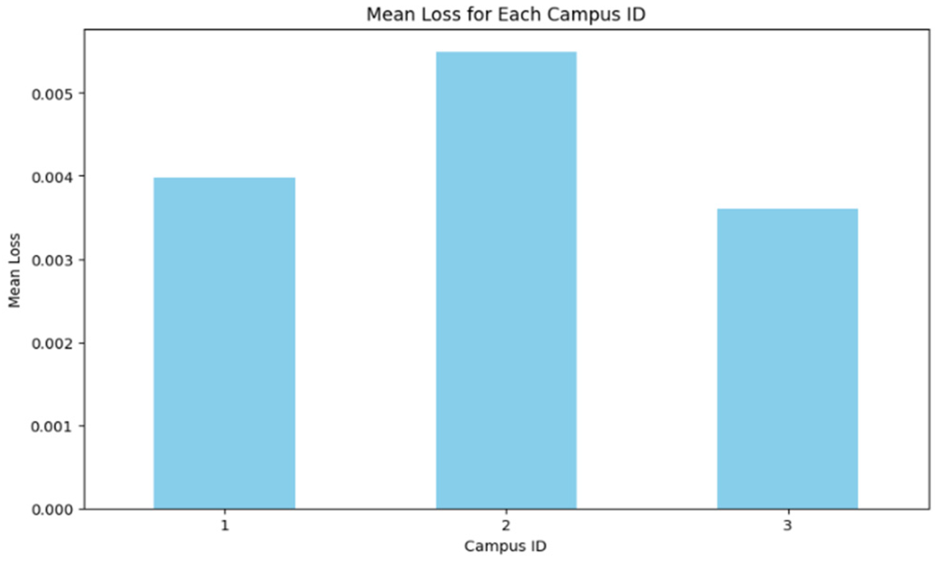
The bar chart included in Figure 10 shows the average loss of all the electricity meters for each campus. Campus 1 shows an average loss of 0.004, indicating relatively accurate energy consumption forecasts. In contrast, Campus 2 shows the highest average loss of 0.005, suggesting higher forecast errors for this campus. Campus 3 shows the lowest average loss of 0.0038, reflecting the minimum detected average loss. These results highlight the variability in predictive performance across campuses and the need to effectively address the unique characteristics and challenges of each campus.

5. Energy Peak Detection Classification

In smart campus environments, the understanding and prediction of energy consumption patterns are essential for implementing effective energy-saving strategies. Detecting peaks in energy consumption is particularly important as they can lead to higher operating costs and increased pressure on the energy infrastructure. Previous studies have explored various methods for detecting peaks in energy consumption data, including statistical approaches such as threshold-based methods, with standard deviation analysis having also been commonly used. Ref. 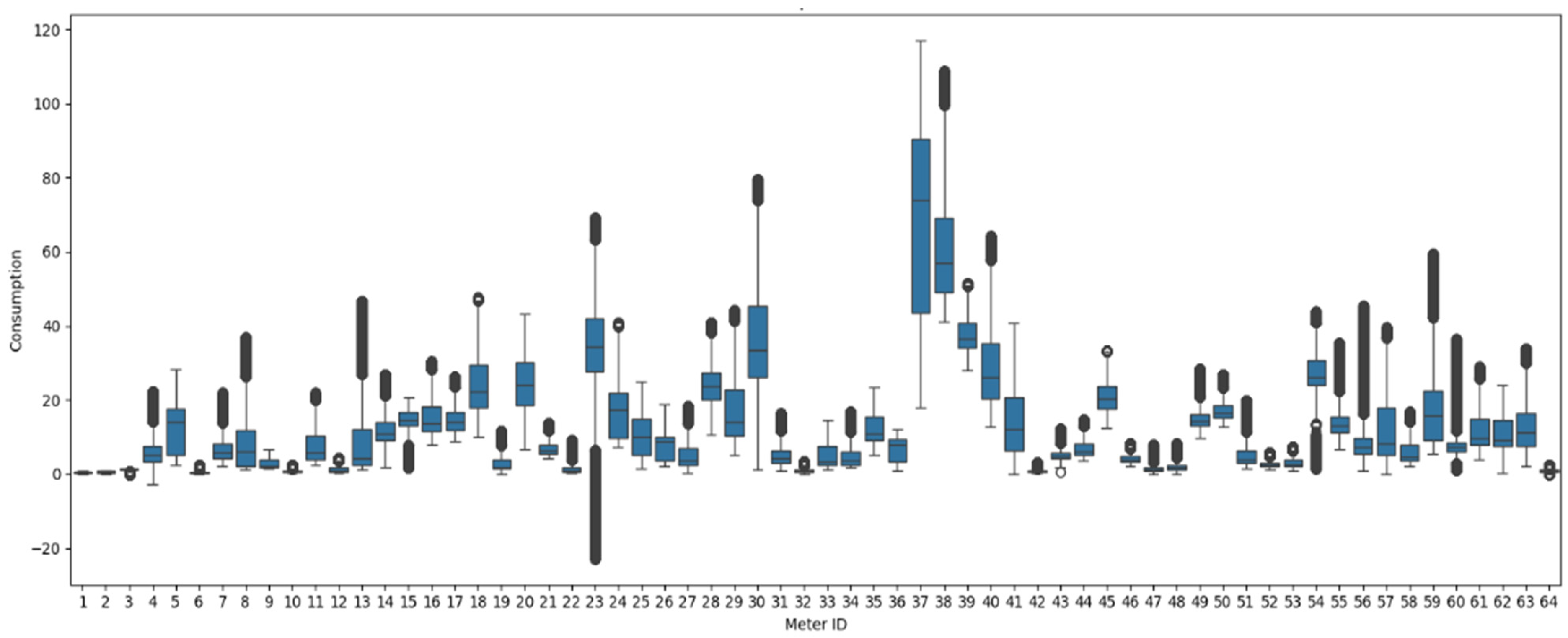[35] applied standard deviation thresholds to identify abnormal energy consumption in residential environments. In this section, we will explain how we employed the use of statistical analysis to identify energy consumption peaks in a smart campus. Through surveying, we hope to categorize the energy flow patterns of each meter, and we seek to hand-craft energy-management policies by analyzing UNICON data of five campuses of La Trobe University. Boxplots present the distribution of data using five measurements (minimum, first quartile (Q1), median, third quartile (Q3), and maximum). We further identify outliers, which in this instance could indicate energy peaks.

Figure 11 illustrates the boxplots for selected meters. The central line in each box represents median energy consumption, providing a measure of central tendency. The edges of the box correspond to Q1 and Q3, indicating the interquartile range (IQR), which encompasses the middle 50% of the data, while whiskers are any points within 1.5 IQR values from quartiles, and points beyond the whiskers are outliers, which are potential peaks. For each meter_id, we implemented an algorithm comprising quartile analysis to label all of the peaks in the energy consumption. The consumption values are classified into four levels by the algorithm as Low, Normal, Extreme, and Danger levels. This classification aids in identifying not only peaks but also periods of unusually low consumption, which could indicate underutilization or sensor malfunctions.

The Algorithm 1 categorizes the data of energy consumption of each meter through the quartile analysis to detect the usage trends and possible anomalies. For each meter_id in the dataset, it extracts the associated consumption data and calculates key statistical measures: the first quartile (Q1), the median (Q2), and the third quartile (Q3). The interquartile range (IQR) is determined by subtracting Q1 from Q3 (IQR = Q3 − Q1). A critical cut-off point is set at Q3 + 1.5 × IQR to find a high consumption value. The algorithm continues by setting each consumption value in the data to one of four categories, depending on relative position to the quartiles: Low in the case that it is less than Q1, Normal in the case that it falls within the range of Q1 and Q3, Extreme in the case that it is greater than Q3 and less than or equal to the extreme threshold, and Danger in the case that it is greater than the extreme threshold. The algorithmic classification of consumption values in such a way can readily identify the times when energy consumption is unusual, which can be used to implement specific measures to reduce energy use and control peak demand. The second step in our study is the incorporation of the system status into an agent system that is driven by large language models (LLMs). This integration will be used to deliver intelligent and adaptive suggestions to conserve energy and increase the efficiency and sustainability of campus operations.

Algorithm 1: CategorizeEnergyConsumption

Input: Dataset containing energy consumption data for multiple meters Output: Categorized energy consumption data with labels: “Low”, “Normal”, “Extreme”, “Danger” Begin   For each meter_id in Dataset do     // Step 1: Extract consumption data for the current meter     data ← GetConsumptionData(meter_id)     // Step 2: Calculate statistical quartiles and IQR     Q1 ← Calculate25thPercentile(data)     Q2 ← Calculate50thPercentile(data) // Median     Q3 ← Calculate75thPercentile(data)     IQR ← Q3 − Q1     // Step 3: Define the extreme threshold     ExtremeThreshold ← Q3 + 1.5 × IQR     // Step 4: Categorize each consumption value     For each consumption_value in data do       If consumption_value < Q1 then         category ← “Low”       Else if Q1 ≤ consumption_value ≤ Q3 then         category ← “Normal”       Else if Q3 < consumption_value ≤ ExtremeThreshold then         category ← “Extreme”       Else         category ← “Danger”       End if       // Step 5: Assign the category to the consumption value       AssignCategory(consumption_value, category)     End for   End for End

6. LLM-Based Multi-Agent System

6.1. Multi-Agent System Architecture and LLMs

LLMs and MASs are at the forefront of automation development in building energy optimization. LLMs have proven to be good at understanding and reasoning with human language. They perform well at processing unstructured information, creating information, and performing complex, language-intensive tasks such as summarizing, responding to queries, and reasoning. However, noisier generic lifecycle management systems have insufficient specific understanding to perform tasks such as energy management, and therefore require additional methods, such as knowledge injection and expert solicitation, to adapt them to the application requirements [36]. On the other hand, MASs are created to delegate work to a network of autonomous agents that can cooperate with each other or act independently to achieve specific goals. MASs are flexible, scalable, and more modular compared to other large and evolved domains such as energy optimization. The incorporation of LLMs into a MAS increases the system’s ability to process unstructured data, be flexible to adapt to different situations, and have knowledge-based and context-dependent decision-making potential. Special functions, such as data pre-processing, performance analysis, or the creation of modernization recommendations, can be applied to LLM-driven agents in relation to other agents and human specialists. In this section, we will explain how we used this LLM-based MAS structure to forecast energy peaks in our smart campus and to develop policies.

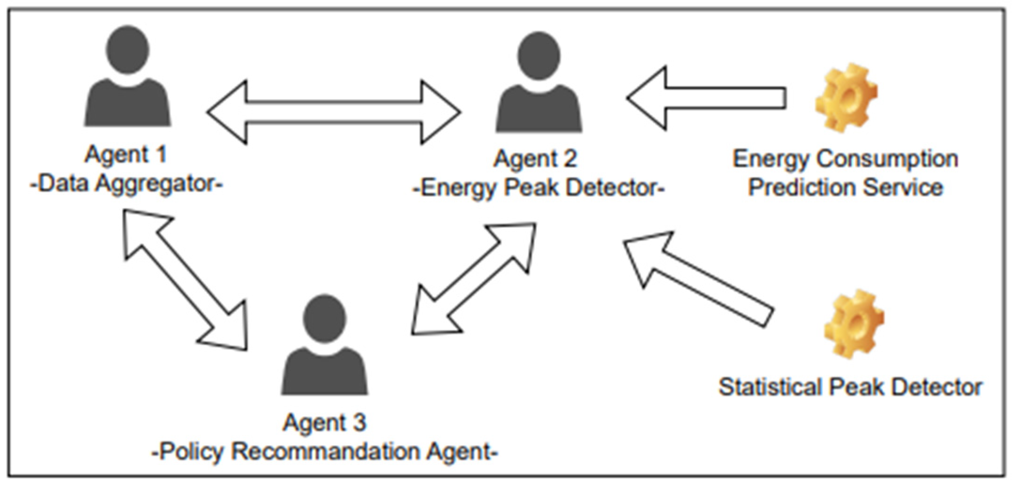
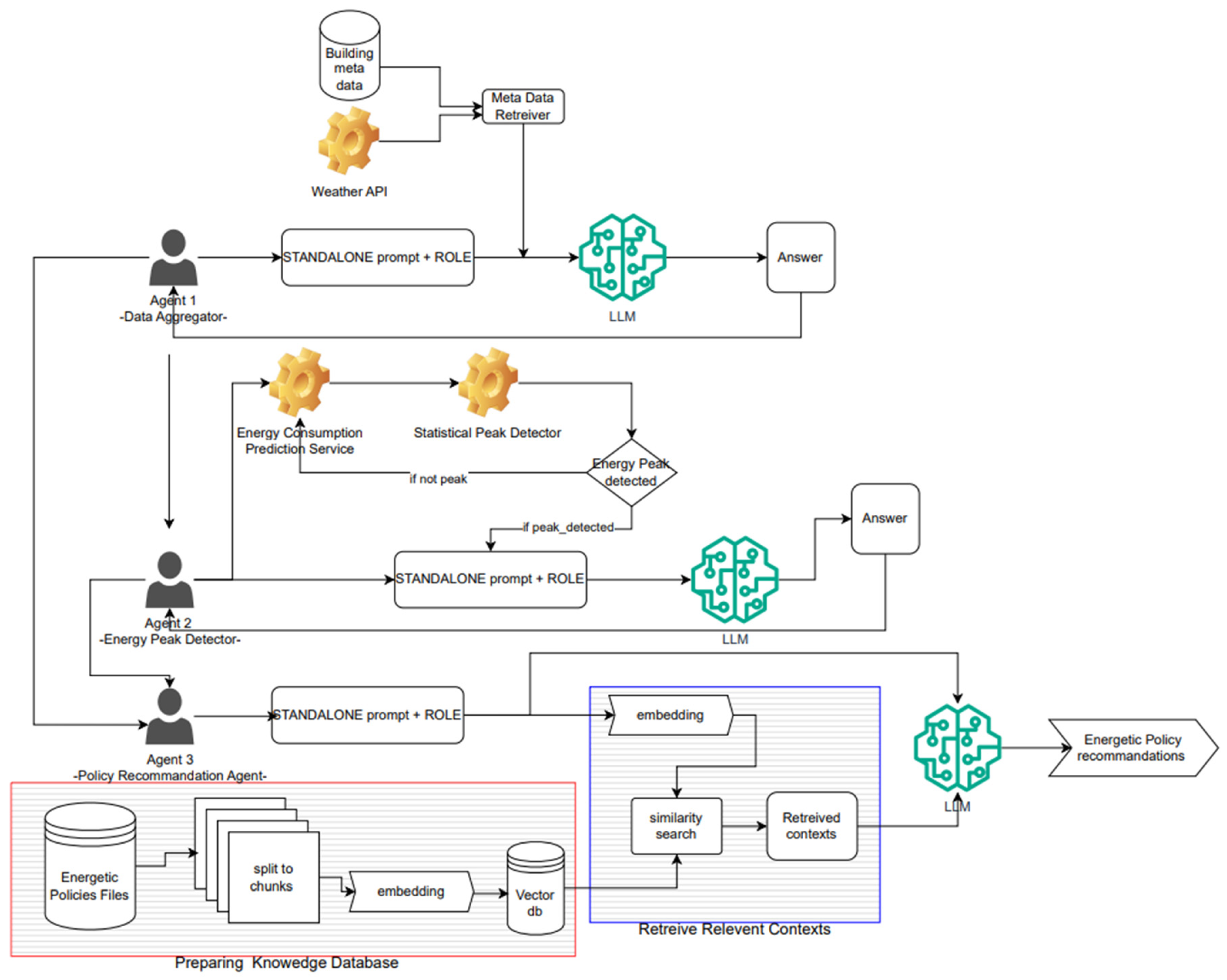
The proposed LLM-powered multi-agent system in Figure 12 is designed to predict demand peaks and generate intelligent policy suggestions specific to smart campuses. By utilizing the advanced natural language understanding and reasoning capabilities offered by large language models (LLMs), the system can efficiently process structured and unstructured data, automate energy management tasks, and provide actionable insights for managing peak loads.

a.

Data Processing: Data Aggregator Agent

The data aggregator agent is responsible for collecting and pre-processing real-time data gathered from different data sources, such as real-time smart meters, weather API, and operating logs. It combines meta-information (time series of energy measurements) with unstructured information like audit reports in a text-based format for an in-depth analysis. Pre-processing is undertaken through the cleaning, normalization, and management of missing or anomalous data points. Using LLMs, the agent can perform sentiment analysis to uncover patterns; for example, from a textual description, an agent can turn the results into actionable intelligence, such as occupancy trend or equipment status. It takes logs of weather data and converts them into defined values like temperature or humidity so that the next agents are provided with good data that is ready to be used.

b.

Forecasting and Peak Detection Agent

The forecasting agent uses the LSTM, GRU, CONV, and hybrid models to ensure the prediction of energy demand in future intervals using context-based data. Once the forecast has been generated, the agent looks for energy peaks using our statistical thresholds algorithm and flags critical energy peaks, triggering the next workflow for generating the policy. Through timely and accurate forecasting and the early detection of peaks, this agent serves as a basis for good recommendations for energy policy.

c.

Policy Recommendation Agent

The policy advisor agent integrates the role of planning and policy generation into one coherent process. When an energy peak is detected, this agent assesses its nature, identifies and prioritizes interventions, such as load shifting, HVAC adjustments, and energy storage deployment, and at the same time, aligns them with operating constraints and resource availability. Using the LLM’s reasoning capabilities, the agent creates these strategies as detailed human-readable policies. The recommendations are provided with justifications, expected outcomes, and trade-offs for the sake of transparency and trust. For example, during a forecasted high demand (peak), during what is expected to be an off-peak hour, the policy advisor agent might suggest scheduling non-critical energy-intensive activities for off-peak hours, changing HVAC setpoints in a less critical area, and alerting building managers and occupants to the required action.

The

Table 1. Description of agent roles, data types, and input sources.

Agents	Input Data Type	Inputs
Data Aggregator	Raw data from various sources	Smart meter readings, weather data, occupancy logs, audit reports, and historical data
Forecasting Agent	Preprocessed, structured data	Time-series energy data, is_holiday, is_event.
Policy Advisor	Forecasted peaks and contextual data	Peak detection results, building constraints, knowledge base inputs, resource status

below summarizes the different agents involved in the proposed system, along with their corresponding input data types and inputs:

The architecture of the LLM component of our multi-agent system is designed to generate energy optimization instructions based on predicted consumption data and data retrieved from our knowledge database. This process involves several interconnected steps that ensure efficient retrieval and application of relevant energy policy information to minimize energy consumption in the smart campus.

The proposed architecture displayed in Figure 13 represents a multi-agent retrieval-augmented generation (RAG) system designed to provide context-aware energy policy recommendations by integrating real-time energy consumption analysis, metadata retrieval, and a structured knowledge database. The system is composed of three key agents, each responsible for a specific task. The first agent represents the metadata acquisition phase. It collects and processes metadata from two primary sources: building metadata, retrieved via a dedicated Metadata Retriever, and weather conditions, fetched using an external Weather API. This information is then structured into a standalone prompt with a predefined role and passed to a large language model (LLM), which generates an initial response based on the contextual data. The second agent is responsible for analyzing energy consumption patterns and identifying peak events. This is achieved through an Energy Consumption Prediction Service, which forecasts expected usage, and a Statistical Peak Detector, which determines whether an energy peak is detected. If no peak is identified, the process terminates at this stage. However, if a peak event is detected, the system constructs another standalone prompt with role-specific instructions and sends it to the LLM, which generates a response about the detected energy peak. The last agent is the policy recommendation agent, which leverages this information to retrieve relevant energy policies from a pre-structured knowledge database. The knowledge database is built from energetic policy files, which are pre-processed into chunks, converted into high-dimensional embeddings, and stored in a vector database for efficient retrieval. When a query is received, the system performs a semantic similarity search within the vector database to retrieve the most relevant policy-related contexts. These retrieved contexts are then incorporated into a final LLM prompt, allowing the model to generate contextually relevant energy policy recommendations based on both real-time analytics and retrieved domain knowledge. This architecture ensures that energy policy recommendations are not only data-driven and fact-based but also dynamically tailored to real-time consumption trends and external environmental factors.

6.2. Evaluation Approach

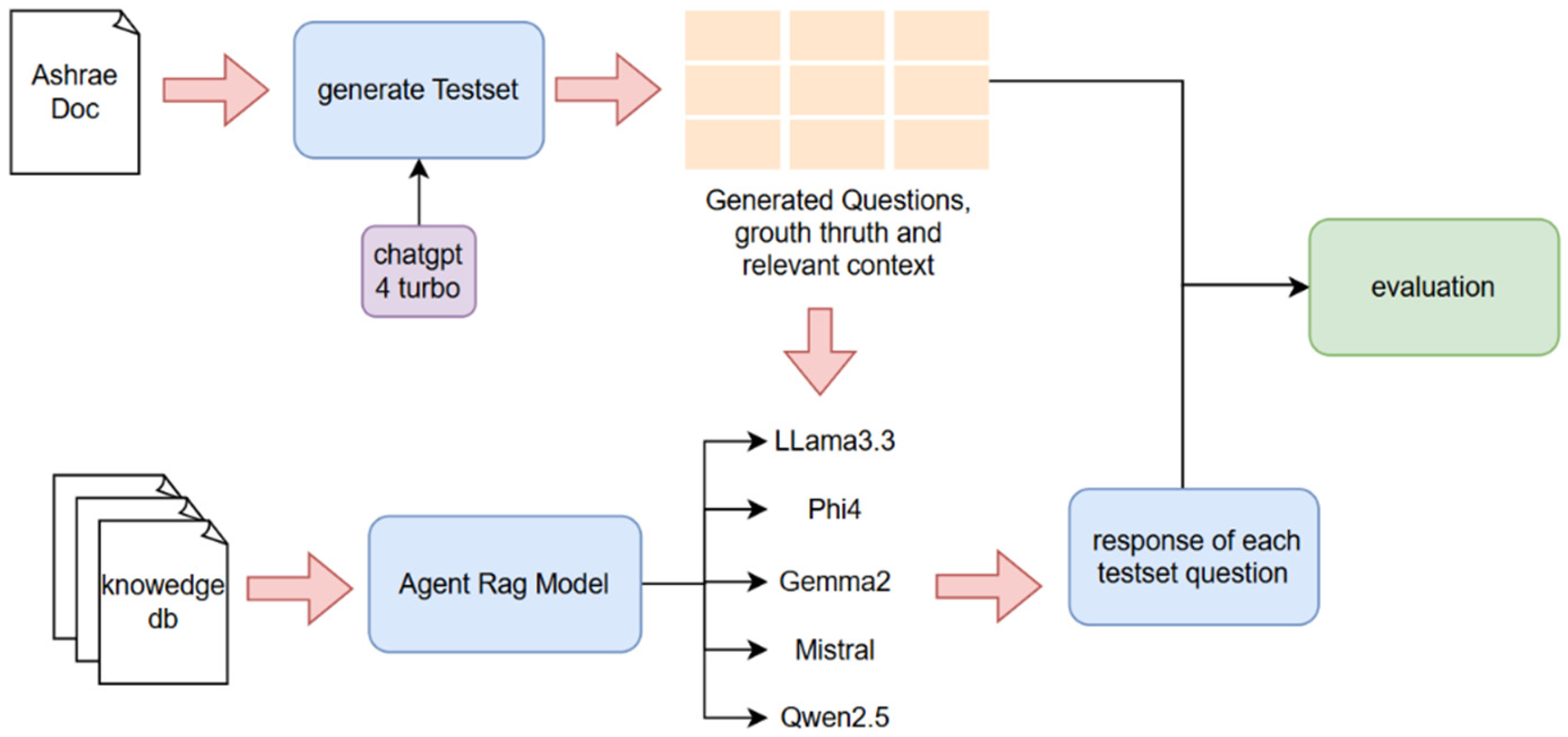
Our evaluation process presented in Figure 14 commenced by curating domain-specific documents, predominantly sourced from authoritative ASHRAE standards; ASHRAE (American Society of Heating, Refrigerating, and Air-Conditioning Engineers) [37] is a global professional organization dedicated to advancing the fields of heating, ventilation, air conditioning, and refrigeration (HVAC&R) through research, standards development, and industry best practices. It sets widely recognized standards and guidelines for energy efficiency, indoor air quality, and building sustainability. These documents were subsequently segmented into 6570 text chunks. To develop a domain-specific test set, the system employs ChatGPT-4 Turbo, which formulates a series of well-structured questions derived from the content of the ASHRAE corpus. Each generated question is systematically linked to a ground-truth reference answer and an associated relevant context, ensuring that the dataset accurately reflects domain-specific knowledge. Once established, the Agent RAG Model utilizes our knowledge database, in which document embeddings are stored to facilitate efficient retrieval. Upon receiving a test question, the model conducts a semantic similarity search within the vectorized knowledge base, retrieving the most contextually relevant chunks. These retrieved segments are then supplied as input to multiple LLMs, including Llama3.3 [25], Phi4 [38], Gemma2 [39], Mistral [40], and Qwen2.5 [41], which process the contextual data to generate corresponding responses. The final phase of the evaluation involves systematically comparing the LLM-generated responses against ground-truth answers and the retrieved contextual information. Performance assessment is conducted using multiple evaluation metrics, including faithfulness (adherence to retrieved context and minimization of hallucinations), correctness (alignment with authoritative ASHRAE knowledge), answer relevancy (degree to which the response directly addresses the posed question), semantic similarity (closeness of the generated response to the reference answer), and context precision/recall (effectiveness in retrieving relevant contextual data). After generating responses using each LLM, the quality of the returned responses is systematically compared, allowing for a quantitative and qualitative assessment of each model’s performance. Based on the evaluation results, the best-performing model is selected as the most suitable for deployment in the domain of energy policy and building efficiency.

6.3. Evaluation Metrics

The evaluation framework for our retrieval-augmented generation (RAG) system incorporates a suite of metrics designed to rigorously assess both the retrieval and generative components of our pipeline.

The faithfulness [42] metric is useful for quantifying how factual the generated response is with regard to the retrieved context, in order to protect against the generation of hallucinations or unsupported assertions. A response is faithful if all the information it makes is completely supported by the retrieved information. The faithfulness score is estimated by citing all different claims in the answer, checking for each of them whether there is a possibility to derive it directly from the retrieved context, and computing the ratio of supported claims to the total number of claims. The formula for faithfulness is given as

$$\mathrm{Faithfulness} ={\displaystyle \frac{\begin{array}{c}\mathrm{N}\mathrm{u}\mathrm{m}\mathrm{b}\mathrm{e}\mathrm{r} \mathrm{o}\mathrm{f} \mathrm{c}\mathrm{l}\mathrm{a}\mathrm{i}\mathrm{m}\mathrm{s} \mathrm{i}\mathrm{n} \mathrm{t}\mathrm{h}\mathrm{e} \mathrm{r}\mathrm{e}\mathrm{s}\mathrm{p}\mathrm{o}\mathrm{n}\mathrm{s}\mathrm{e} \mathrm{s}\mathrm{u}\mathrm{p}\mathrm{p}\mathrm{o}\mathrm{r}\mathrm{t}\mathrm{e}\mathrm{d}\\ \mathrm{b}\mathrm{y} \mathrm{t}\mathrm{h}\mathrm{e} \mathrm{r}\mathrm{e}\mathrm{t}\mathrm{r}\mathrm{i}\mathrm{e}\mathrm{v}\mathrm{e}\mathrm{d} \mathrm{c}\mathrm{o}\mathrm{n}\mathrm{t}\mathrm{e}\mathrm{x}\mathrm{t}\end{array}}{\mathrm{Total} \mathrm{number} \mathrm{of} \mathrm{claims} \mathrm{in} \mathrm{the} \mathrm{response}}}$$

(6)

where scores range from 0 to 1, with higher values indicating stronger factual alignment. A low faithfulness score suggests that the response introduces hallucinated information, reducing reliability.

Alongside this, context precision assesses the proportion of relevant chunks among the retrieved contexts by computing Precision@k, which is the ratio of true positives to the sum of true positives and false positives, expressed as

$$\mathrm{Precision}@\mathrm{k}={\displaystyle \frac{\mathrm{true} \mathrm{positives}@\mathrm{k}}{\left(\mathrm{true} \mathrm{positives}@\mathrm{k}+\mathrm{false} \mathrm{positives}@\mathrm{k}\right)}}$$

(7)

and Context Precision@K aggregates these values across the top-k retrieved results:

$$\mathrm{Context} \mathrm{Precision}@\mathrm{K}={\displaystyle \frac{\sum _{k=1}^K\left(\mathrm{Precision}@\mathrm{k}\times v_k\right)}{\mathrm{Total} \mathrm{number} \mathrm{of} \mathrm{relevant} \mathrm{items} \mathrm{in} \mathrm{the} \mathrm{top} K \mathrm{results}}}$$

(8)

where higher values indicate better retrieval accuracy. Complementary to this, context recall [43] evaluates how well the retrieval system captures all relevant information, ensuring no critical data is omitted. It is computed as

$$\mathrm{Context} \mathrm{Recall}={\displaystyle \frac{\begin{array}{c}\mathrm{N}\mathrm{u}\mathrm{m}\mathrm{b}\mathrm{e}\mathrm{r} \mathrm{o}\mathrm{f} \mathrm{c}\mathrm{l}\mathrm{a}\mathrm{i}\mathrm{m}\mathrm{s} \mathrm{i}\mathrm{n} \mathrm{t}\mathrm{h}\mathrm{e} \mathrm{r}\mathrm{e}\mathrm{f}\mathrm{e}\mathrm{r}\mathrm{e}\mathrm{n}\mathrm{c}\mathrm{e} \mathrm{s}\mathrm{u}\mathrm{p}\mathrm{p}\mathrm{o}\mathrm{r}\mathrm{t}\mathrm{e}\mathrm{d} \\ \mathrm{b}\mathrm{y} \mathrm{t}\mathrm{h}\mathrm{e} \mathrm{r}\mathrm{e}\mathrm{t}\mathrm{r}\mathrm{i}\mathrm{e}\mathrm{v}\mathrm{e}\mathrm{d} \mathrm{c}\mathrm{o}\mathrm{n}\mathrm{t}\mathrm{e}\mathrm{x}\mathrm{t}\end{array}}{\mathrm{Total} \mathrm{number} \mathrm{of} \mathrm{claims} \mathrm{in} \mathrm{the} \mathrm{reference}}}$$

(9)

where higher recall scores indicate more comprehensive retrieval. Moving to the generative aspects, answer relevancy quantifies how well the generated response aligns with the original question, using cosine similarity between the original question embedding and a set of reverse-engineered questions derived from the response:

$$\mathrm{A}\mathrm{nswer} \mathrm{relevancy}={\displaystyle \frac{1}{N}}{\sum }_{i=1}^N\cos \left(E_{g_i},E_o\right)$$

(10)

$$\mathrm{Answer} \mathrm{relevancy}={\displaystyle \frac{1}{N}}{\sum }_{i=1}^N{\displaystyle \frac{E_{g_i}\cdot E_o}{‖E_{g_i}‖‖E_o‖}}$$

(11)

where E_gi is the embedding of the generated question iii, E_o is the embedding of the original question, and N is the number of generated questions. A higher score indicates that the response remains highly relevant to the query, while a low score suggests off-topic or incomplete answers. Answer correctness is determined by comparing the generated response to the ground truth, incorporating factual correctness through an answer correctness score, calculated as

$$\mathrm{Answer} \mathrm{Correctness} \mathrm{Score}={\displaystyle \frac{|\mathrm{TP}|}{\left(\left|\mathrm{TP}\right|+0.5\times \left(\left|\mathrm{FP}\right|+\left|\mathrm{FN}\right|\right)\right)}}$$

(12)

where TP (True Positives) are facts correctly present in both the generated response and the ground truth, FP (False Positives) are incorrect statements in the response, and FN (False Negatives) are missing details from the ground truth. Finally, semantic similarity quantifies how closely the meaning of the generated response aligns with the reference answer, regardless of wording differences, calculating the cosine between the generated response embedding and the reference response embedding, where higher scores indicate that the generated response retains the intended meaning of the reference answer.

7. Results

Within the context of our comparative analysis, we considered five advanced large language models (LLMs) with different architectures. Qwen-2.5 is a 13 billion-parameter model that demonstrates a strong ability in multilingual tasks and domain-specific applications like finance and healthcare due to its broad pretraining on large datasets and fine-tuning. LLaMA-3.3, a 14-billion-parameter model, is fine-tuned for open-ended dialog and instruction-following use cases based on a refined reinforcement learning from human feedback (RLHF) mechanism that helps improve alignment with the user’s intent. We also tested Mistral-3, which is a model with 36 billion parameters with a sliding window close-attention, which substantially minimizes computation costs and still achieves high quality in text generation and summarization tasks, thus being suitable for low-latency applications. Phi-4 is a small 1.3 billion-parameter model for reasoning and coding tasks, leveraging a data-optimized training pipeline that prioritizes high-quality textbook-like data to attain powerful performances with a lower range of size. Lastly, a 2.5 billion parameter model called Gemma-2 is built specifically around ethical AI to this end, with a strong safety filter and mitigating bias, while retaining support for competitive general NLP benchmarks.

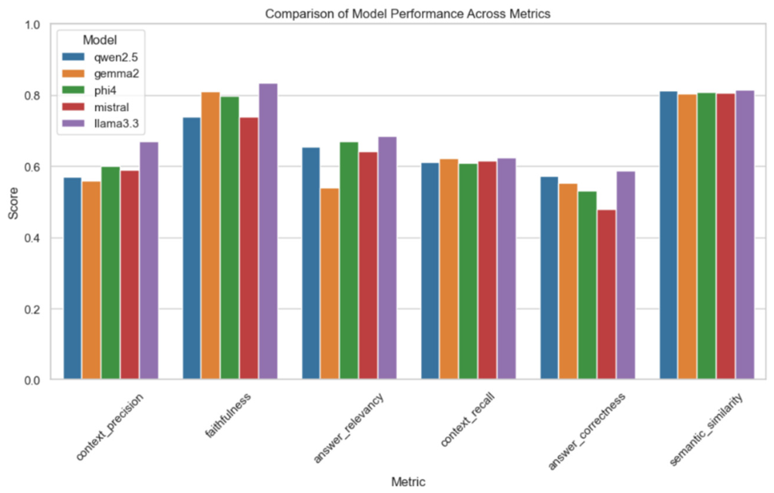
For a better comparison of large language models with respect to these six key performance metrics context precision, faithfulness, answer relevancy, context recall, answer correctness, and semantic similarity we conducted an evaluation of five large language models, namely Qwen2.5, Gemma2, Phi4, Mistral, and Llama3.3. Llama3.3 showed better performance compared to the other models in the overall case.

Context precision, which evaluates the proportion of relevant retrieved chunks, as mentioned in Figure 15 and

Table 2. Quantitative evaluation of RAG models on multiple metrics.

Models	Context Precision	Faithfulness	Answer Relevancy	Context Recall	Answer Correctness	Semantic Similarity
Qwen2.5	0.57	0.7389	0.6551	0.6107	0.5721	0.812
Gemma2	0.56	0.8098	0.5401	0.6223	0.5523	0.8031
Phi4	0.6	0.7977	0.6705	0.6103	0.5313	0.8083
Mistral	0.59	0.7402	0.6412	0.6153	0.4801	0.8062
Llama3.3	0.66	0.8339	0.6551	0.619	0.5884	0.8151

is highest for Llama3.3 (0.66), followed by Phi4 (0.60) and Mistral (0.59), while Gemma2 scores the lowest (0.56), indicating that Llama3.3 consistently retrieves more relevant information, reducing the risk of incorporating irrelevant data. Faithfulness, measuring factual consistency with the retrieved context, is also highest for Llama3.3 (0.8339), followed closely by Gemma2 (0.8098) and Phi4 (0.7977), suggesting that these models generate more factually grounded responses with minimal hallucination, whereas Mistral (0.7402) shows weaker faithfulness, meaning it occasionally includes unsupported claims. Answer relevancy, which assesses how well the response aligns with the question, highlights Phi4 (0.6705) as the best model, followed by Llama3.3 (0.6551) and Qwen2.5 (0.6551), whereas Gemma2 (0.5401) ranks the lowest, suggesting that it sometimes fails to fully address the question. context recall, which ensures all relevant information is retrieved, remains balanced across models, with Gemma2 achieving the highest recall (0.6223), followed closely by Llama3.3 (0.6153), Mistral (0.6153), and Qwen2.5 (0.6107), showing that most models retrieve a sufficient amount of relevant information with minor differences. However, answer correctness, which determines factual accuracy by comparing responses to the ground truth, shows significant variation, with Llama3.3 achieving the highest score (0.5884), followed by Qwen2.5 (0.5721), while Mistral (0.4801) scores the lowest, indicating that Mistral tends to generate incorrect responses more frequently. Lastly, semantic similarity, which measures how closely the generated response matches the ground truth meaning, is relatively high across all models, with Llama3.3 (0.8151) achieving the best score, followed closely by Qwen2.5 (0.812), Phi4 (0.8083), and Mistral (0.8062), suggesting that all models generate semantically coherent responses, even though some may introduce factual inaccuracies.

8. Discussions

The comparative results demonstrate that LSTM and CNN-LSTM architectures consistently outperform GRU and GRU+CNN across multiple meters. This is in agreement with previous research showing that hybrid convolutional–recurrent networks can extract spatial features before modeling temporal dependencies and thereby achieve lower MSE, MAE, and RMSE values than standalone CNN or LSTM. For example, Khan et al. [44] found that combining CNN and LSTM reduced MSE from 0.35 (LSTM) to 0.31 and further to 0.007 at daily resolution, outperforming other deep-learning models Such hybrids are effective because CNN layers capture local temporal patterns while LSTM layers model long-term dependencies. The variability in mean loss across campuses underscores the influence of building type, occupancy patterns, and external factors (weather, holidays).

The quartile-based classification scheme provides a simple yet robust way to flag consumption peaks. Statistical boxplots are widely used to detect anomalies because they are robust to outliers and do not assume any particular distribution. By converting continuous consumption values into categorical labels (Low, Normal, Extreme, Danger), the system can identify times when proactive demand-response actions are necessary. However, these thresholds are purely statistical and may not align with contractual or economic peak limits; integrating tariff-specific thresholds or demand charges would improve practical relevance.

Based on this evaluation of our policy recommendation agent’s output, Llama3.3 emerges as the most robust model, excelling in context precision, faithfulness, answer correctness, and semantic similarity, while also maintaining competitive scores in context recall and answer relevancy, making it the most reliable model for generating fact-based, contextually relevant responses. Although Phi4 performs best in answer relevancy, it falls short in recall and correctness, making it less reliable for precise knowledge retrieval tasks. Similarly, Gemma2 demonstrates strong faithfulness but ranks lower in answer relevancy and correctness, indicating that while it stays grounded in retrieved information, it may not always provide the most relevant or complete answers. Mistral, with the lowest answer correctness score (0.4801), is the weakest performer overall, as it is more prone to generating incorrect or misleading responses, making it less suitable for high-precision applications. Consequently, Llama3.3 is the most suitable model for deployment in knowledge-intensive RAG systems, as it consistently retrieves high-quality information, generates factually accurate responses, and maintains strong semantic alignment with authoritative references. In terms of sustainability, an increasing amount of work in the literature confirms that more AI-aspired energy management will not only save money but also enhance the sustainability score in a university setting. Madabathula et al. [45] has recently suggested an example of a smart green energy management system, which combines machine learning prediction with reinforcement learning control to optimize electricity consumption and solar generation within a campus; the system has a better prediction accuracy and provides a scalable solution that is not bound to external grids and is more energy efficient.

Based on these findings, our multi-agent framework integrates per-meter prediction, median-based peak prediction, and policy suggestions provided by LLM so that demand response may take context-dependent responses. Our approach can be used to minimize the costs of energy by focusing on the consumption peaks and ensuring that when a shift or a reduction in loads is required, it is able to recommend it. Furthermore, we will track the energy, latency, and carbon footprint of our forecasting and LLM elements and compare and contrast them with the performance of lighter-weight models to confirm that the benefits of operation are not paying a huge operational price.

After all, we envision several enhancements, including the domain-specific fine-tuning of LLMs using the corpora of energy regulations and operational data; integration of reinforcement learning for policy feedback; coupling the multi-agent system with a digital-twin environment for closed-loop simulations; adding renewable-energy agents to dynamically manage on-site generation and storage; exploring multi-objective optimization to balance cost, comfort, and emissions; and developing more interpretable LLM architectures. These perspectives point to promising avenues for advancing smart campus energy management.

9. Conclusions

This paper presents a time-series forecast with an LLM multi-agent layer to manage energy consumption on smart campuses. We modeled consumption forecasting again with LSTM, CNN-LSTM, GRU, and hybrid models, and we selected the model with the least loss. We separated peak from base demand using a median-based threshold to facilitate our actions at the times we feel it is most useful. We also evaluated a RAG pipeline that uses our multi-agent system on five new LLMs, Qwen2.5, Gemma2, Phi4, Mistral, and Llama3.3, with six metrics: context precision, faithfulness, response relevance, context recall, response correctness, and semantic similarity. Llama3.3 had the highest context values, with 0.66 precision and 0.8339 faithfulness, along with an accuracy of 0.5884 and an overall semantic similarity of 0.8151, across its responses. This suggests that it has a solid ability to search and provide helpful recommendations for on-topic responses. The multi-agent framework then drives the actions. The data aggregator agent cleans and combines the potential streams from smart meters, weather, and operations logs into a single stream. The forecasting agent marks likely peaks, while the policy recommendation agent, which can be improved, recommends selected actionable steps using RAG and a knowledge base. This approach produced largely favorable outcomes across faithfulness, correctness, answer relevancy, semantic similarity, and retrieval precision/recall metrics, signifying that good retrieval leads to the successful generation of evidence-based policies. Again, Llama3.3 had the most favorable outcomes here; however, it might be improved with some light domain fine-tuning to work through context nuances.