Explainable AI for Water Leakage Detection in Urban Water Distribution Networks Using Real and Simulated Data

Abstract

Water leakage in urban water distribution networks (WDNs) poses significant challenges for sustainable resource management and infrastructure reliability. Traditional detection methods are often reactive and difficult to scale in modern sensor-rich environments. This paper proposes a hybrid data-driven framework for early leak detection that integrates physics-informed simulation with machine learning and explainable analytics. A region-aware EPANET-style simulator is developed to generate realistic hydraulic data under varying demand patterns, environmental conditions, and pressure-dependent leak scenarios. To enhance generalizability, the synthetic dataset is combined with a BATADAL-inspired benchmark, enabling both in-domain and cross-domain evaluation. A feature engineering pipeline is introduced to capture temporal, spatial, and hydraulic relationships, expanding raw sensor signals into a high-dimensional representation. Six machine learning models, including Random Forest, Gradient Boosting, Support Vector Machine, Logistic Regression, Isolation Forest, and a PCA-Based Autoencoder, are systematically evaluated under constrained false-positive requirements. The results show that tree-based ensemble models achieve strong detection performance while maintaining low false-alarm rates (FPR ≤ 0.05). Importantly, cross-domain experiments demonstrate that models trained on simulated data retain competitive performance when applied to benchmark datasets, indicating robust transferability. Finally, explainability analysis reveals that pressure-based temporal statistics and spatial gradients are key indicators of leakage, providing interpretable insights for system monitoring. The proposed framework offers a scalable and generalizable approach for intelligent leak detection in modern water distribution systems.

1. Introduction

Water is a critical natural resource underpinning public health, food security, industrial development, and ecosystem sustainability. However, freshwater availability is increasingly constrained due to population growth, urbanization, and climate change. Recent global assessments indicate that more than two billion people live in water-stressed regions, a number expected to rise in coming decades [1]. In this context, efficient management of water distribution infrastructure is essential. One of the most pressing challenges is non-revenue water (NRW), defined as the difference between water supplied and water billed. Global NRW levels typically range between 35% and 45%, with physical leakage accounting for a substantial portion of these losses [2]. Beyond economic impact, leakage contributes to infrastructure degradation, pipe corrosion, and contamination risks, while increasing energy consumption in pumping systems [3].

The challenge of NRW is particularly severe in water-scarce and arid regions, where water production is often energy-intensive and costly. For example, countries relying heavily on desalination face significant economic and environmental burdens associated with water losses [4]. In such contexts, reducing leakage is not only a matter of efficiency but also of sustainability. Large-scale distribution networks operating under harsh environmental conditions—such as high temperatures and long transmission distances—further complicate leak detection due to increased mechanical stress on pipelines and complex hydraulic dynamics [5,6]. These factors highlight the need for robust and adaptive detection mechanisms capable of operating under diverse and challenging conditions.

Traditional approaches to leak detection have relied primarily on physical sensing techniques such as acoustic correlators, negative pressure wave analysis, and minimum night flow (MNF) methods [2,3,6]. While these methods have proven effective for detecting large and abrupt burst events, they suffer from several inherent limitations. First, they are generally insensitive to small or gradual leaks, which constitute the majority of physical losses in ageing infrastructure systems. Second, their deployment requires manual intervention by specialized personnel, making continuous real-time monitoring impractical in large-scale networks. Third, their effectiveness is significantly reduced in modern pipeline materials, particularly plastic pipes, and under high-temperature conditions where acoustic signals attenuate more rapidly [3]. Furthermore, these approaches do not scale efficiently with the increasing size and complexity of modern urban water networks, limiting their applicability in smart city environments. These limitations highlight the need for more scalable, automated, and data-driven approaches capable of operating under the complex conditions observed in contemporary urban water systems.

The rapid advancement of Internet of Things (IoT) technologies and the increasing deployment of supervisory control and data acquisition (SCADA) systems have transformed water distribution networks into data-rich environments. Modern systems continuously collect high-resolution measurements from pressure sensors, flow meters, and other monitoring devices, generating multivariate time-series data streams that capture the dynamic behavior of hydraulic systems [7]. Machine learning techniques offer a powerful framework for analyzing such data, enabling the automatic identification of patterns associated with normal operation and the detection of deviations indicative of anomalies or leaks. Supervised learning methods, including Random Forests, Support Vector Machines, and gradient boosting algorithms, have demonstrated high accuracy when trained on labeled datasets containing historical leak events [8]. In contrast, unsupervised approaches such as autoencoders and Isolation Forests are particularly valuable in scenarios where labeled anomaly data is scarce, as they can learn normal system behavior and identify outliers without explicit supervision [9]. Additionally, recurrent neural network architectures, such as Long Short-Term Memory (LSTM) models, have shown promise in capturing temporal dependencies in sensor data, further improving detection performance in dynamic environments [10].

Despite these advancements, several critical limitations remain in the current body of research. A major challenge is the limited availability of representative datasets for diverse environmental conditions [11]. Existing benchmark datasets, most notably the BATADAL dataset, are based on synthetic models of Western urban networks and do not reflect the climatic, operational, and infrastructural characteristics of Saudi systems. This lack of representative data introduces a significant barrier to the development and validation of region-specific detection models. Furthermore, many existing simulation frameworks rely on standard demand patterns and environmental assumptions derived from temperate regions, resulting in models that fail to capture the unique dynamics of high-temperature, high-variability environments [12]. Another important limitation is the lack of explainability in many machine learning-based detection systems. While high classification accuracy is often reported, these models frequently operate as black boxes, providing little insight into the underlying causes of detected anomalies. This lack of transparency reduces trust among utility operators and limits the practical adoption of such systems [13,14]. Finally, most studies do not evaluate cross-domain generalization, which is critical for real-world deployment.

To address these challenges, this study proposes a comprehensive framework, termed HydroDetect-SA, for water leakage detection in Saudi urban distribution networks. The proposed approach integrates a parametrized hydraulic simulation environment with machine learning-based anomaly detection and explainable analytics. Specifically, a customized EPANET-style simulator is developed to generate realistic time-series data under region-specific conditions, incorporating regionally calibrated demand patterns, extreme temperature variations, and pressure-dependent leak scenarios. This synthetic dataset is combined with a BATADAL-inspired benchmark to enable both in-domain and cross-domain evaluation, thereby addressing the data scarcity problem while maintaining statistical realism. A physics-informed feature engineering pipeline is introduced to capture both temporal and spatial characteristics of hydraulic behavior, including rolling statistics, differential features, pressure gradients, and pressure–flow relationships. Multiple machine learning models, spanning supervised, unsupervised, and reconstruction-based paradigms, are systematically evaluated to identify the most effective detection strategies. In addition, a structured ablation study and cross-dataset generalization analysis are conducted to quantify feature importance and model robustness. Finally, an explainability module based on feature importance metrics and SHAP analysis is incorporated to provide interpretable insights into model predictions, supporting practical deployment and decision-making in real-world utility operations.

1.1. Traditional Hydraulic Methods

Pipe leak detection in WDNs has historically relied on physics-based and signal-processing approaches developed well before the emergence of data-driven methods. Acoustic methods remain widely used but suffer from signal attenuation and reduced sensitivity under certain conditions [3]. Hydraulic-based techniques such as negative pressure wave (NPW) analysis and minimum night flow (MNF) provide practical detection mechanisms but require controlled conditions and lack real-time scalability [2,6]. Pressure-driven and model-based approaches have also been widely studied and have demonstrated effectiveness in real-world systems [15,16].

1.2. Machine Learning Methods

The application of machine learning (ML) to water distribution systems has gained significant traction over the past decade, offering a data-driven alternative to traditional approaches. Early work by [5] represents one of the first systematic applications of neural networks for anomaly detection in WDNs. Using flow time-series data from UK district metered areas, they demonstrated detection rates exceeding 85% for significant burst events. Subsequent research has explored a range of supervised learning techniques. Authors in [17] proposed a hybrid approach combining Support Vector Machines (SVM) with residual signals derived from EPANET-based hydraulic models. This integration of physics-based and data-driven features enabled accurate leak localization in simulated environments, achieving classification accuracies above 90%. Similarly, [8] conducted a comparative study of multiple classifiers, including decision trees, SVM, and Random Forest (RF), concluding that RF consistently performed better than other models due to its robustness to noise, ability to handle high-dimensional data, and inherent feature importance estimation capabilities.

1.3. Deep Learning Methods

Deep learning has recently emerged as a powerful tool for modeling complex, nonlinear relationships in WDN data. Unlike ML methods, deep neural networks can automatically learn hierarchical feature representations directly from raw sensor inputs. Architectures such as autoencoders and graph neural networks effectively model nonlinear relationships and network topology. A study has shown strong performance in anomaly and burst detection tasks [10]. Unsupervised deep learning approaches have also been widely explored. In [9], proposed a stacked autoencoder trained exclusively on normal operating data, using reconstruction error as an anomaly score. This approach achieved strong performance without requiring labeled leak data, making it particularly attractive for real-world deployments where anomalies are rare. Similarly, Long Short-Term Memory (LSTM) networks [18] have been applied to model temporal dependencies in pressure and flow time-series. These models can capture multi-step temporal patterns, enabling early detection of gradual leaks that may not be apparent in instantaneous measurements. In [19], authors further demonstrated the effectiveness of LSTM models in water demand forecasting and proposed a framework that shows LSTM’s ability to capture diurnal consumption patterns.

1.4. Hybrid Methods

Recent studies emphasize hybrid approaches integrating physical models with data-driven methods. For example, Soldevila et al. [17] combined residual-based modeling with machine learning for improved leak localization, while pressure-based monitoring techniques have been extensively reviewed for their effectiveness [15]. Search-space reduction methods improve localization efficiency in real systems [20], and deep learning models have demonstrated strong performance in identifying burst events [21]. Additionally, model-based approaches using pressure sensors have shown practical feasibility in operational networks [16].

1.5. XAI Methods

As machine learning models become increasingly complex, the need for interpretability has gained significant attention, particularly in safety-critical domains such as water infrastructure. Explainable AI (XAI) techniques aim to provide insights into model predictions, enabling operators to understand and trust automated decisions. Ribeiro et al. [14] introduced Local Interpretable Model-Agnostic Explanations (LIME), which approximates complex models with simple local surrogates to explain individual predictions. Lundberg and Lee [22] later proposed SHAP (SHapley Additive exPlanations), a theoretically grounded approach based on cooperative game theory that provides consistent and globally interpretable feature attributions.

More recent studies have emphasized the role of explainability in water infrastructure monitoring. Vaquet et al. [23] provide a structured survey of machine learning applications in water distribution networks, highlighting leakage detection and localization as benchmark tasks where explainability is critical. While Salih et al. [24] discuss the strengths and limitations of SHAP and LIME in tabular domains, noting their applicability to safety-critical infrastructure monitoring tasks such as water systems. These recent contributions reinforce the importance of transparent feature attribution and motivate our integration of SHAP-based explanations in HydroDetect-SA.

1.6. BATADAL Dataset and EPANET Simulation

Benchmark datasets and simulation tools play a crucial role in the development and evaluation of leak detection algorithms. The BATADAL dataset [11], introduced as part of an international competition, is widely regarded as a benchmark dataset for anomaly and cyber-physical attack detection in water distribution networks and has been extensively adopted in subsequent studies evaluating machine learning and deep learning approaches. Recent systematic reviews report that approximately one-third of published studies in this area utilize BATADAL, highlighting its prominence as a community benchmark [25]. EPANET [12], developed by the U.S. Environmental Protection Agency, is the most widely used tool for hydraulic simulation of water distribution systems. It implements extended-period simulation of flow and pressure using the gradient method and supports detailed modeling of network components. The Water Network Tool for Resilience (WNTR) [26] extends EPANET functionality through a Python interface, enabling programmatic simulation, uncertainty analysis, and synthetic data generation. These tools have been extensively used to create training datasets for ML models in the absence of real-world data [13].

1.7. Research Gap

Despite significant progress, existing studies exhibit several limitations, including limited dataset diversity, insufficient cross-domain validation, and lack of interpretability. These gaps motivate the development of hybrid, simulation-driven, and explainable frameworks for robust leak detection across diverse operational conditions.

The main contributions of this work are:

• A hybrid EPANET-based simulation and benchmark framework is developed for realistic and cross-domain water leakage detection in urban water distribution networks.
• Multiple machine learning models are systematically evaluated to analyze leak detection performance, robustness, and transferability across simulated and benchmark datasets.
• An explainable and physics-informed analytics pipeline is introduced to identify key hydraulic indicators of leakage and provide interpretable insights for intelligent water network monitoring.

2. Proposed Work

2.1. Formal Definition

Let $s=\left\{\begin{array}{c}{s}_1,s_2,s_3, \dots , s_M\end{array}\}\right.$ denote a set of $M=20$ sensors deployed across a WDN, where each sensor corresponds to either a pressure or flow measurement point. At each discrete time step $t$, sensor $S_i$ records a scalar observation $x_i^{\left(t\right)}\in R,$ representing the instantaneous hydraulic state at that location. Collectively, these measurements form a multivariate time-series representation of the network.

$$x^{\left(t\right)}={\left[x_1^{\left(t\right)},x_2^{\left(t\right)},\dots ,x_M^{\left(t\right)}\right]}^T\in R^M$$

To enhance the representational capacity of raw sensor signals, a feature engineering transformation is applied, mapping the original measurements into a higher-dimensional feature space that captures temporal, spatial, and statistical characteristics of the system:

$${\mathsf{\varphi }}^{\left(\mathit{t}\right)}\in {\mathit{R}}^{\mathit{D}}, \mathit{D}\gg \mathit{M}$$

The supervised learning dataset is then defined as:

$$\mathcal{D}=\{\left({\mathsf{\varphi }}^{\left(\mathit{t}\right)},{\mathit{y}}^{\left(\mathit{t}\right)}\right){\}}_{\mathit{t}=\mathbf{1}}^{\mathit{T}}, {\mathit{y}}^{\left(\mathit{t}\right)}\in \{\mathbf{0},\mathbf{1}\}$$

(1)

where $y^{\left(t\right)}= 1$ indicates the presence of a leak event, and $y^{\left(t\right)}= 0$ corresponds to normal system operation.

The objective is to learn a mapping function fθ(⋅), parameterized by θ, which predicts the system state:

$$\widehat{y^{\left(t\right)}}=f_{\theta }\left({\varphi }^{\left(t\right)}\right)$$

(2)

This formulation corresponds to a binary classification problem, where the model must distinguish subtle deviations in hydraulic behavior caused by leaks from normal operational variability.

Model training minimizes cross-entropy loss, while model selection is performed based on maximizing F1-score under an operational FPR constraint. Class imbalance (2.84:1 to 3.24:1) is addressed through inverse-frequency class weights.

2.2. System Architecture

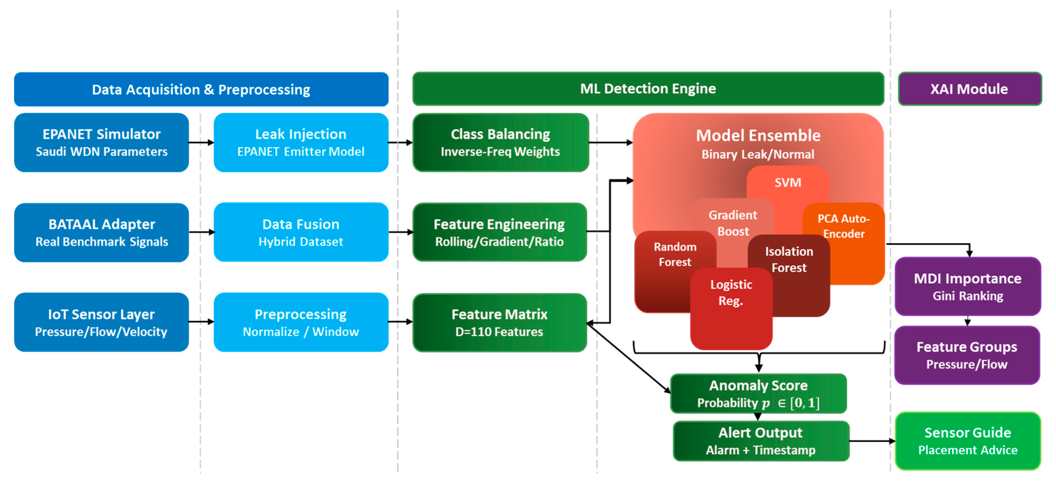
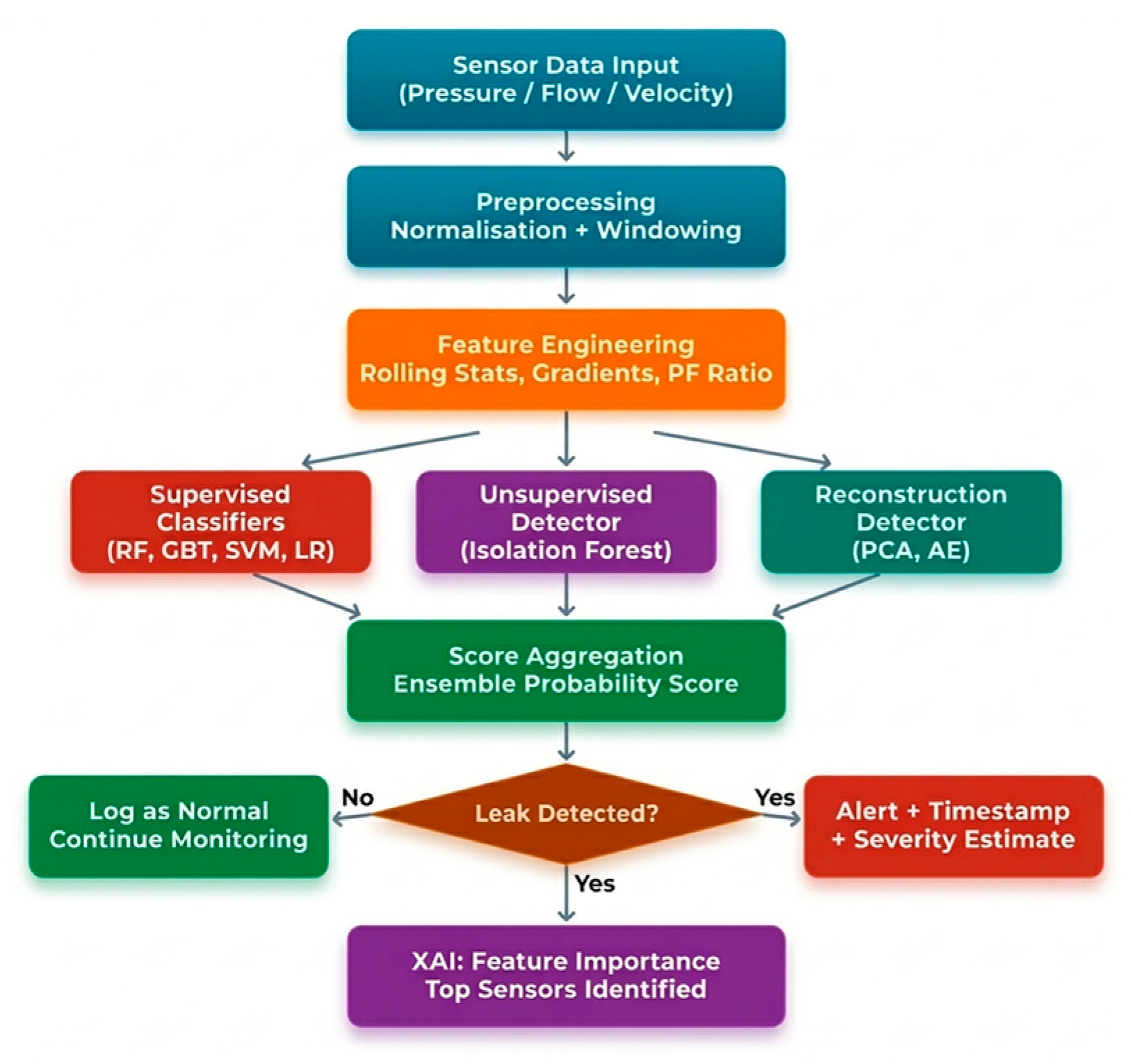
The overall architecture of the proposed HydroDetect-SA framework is illustrated in Figure 1, which presents the three-stage pipeline from data acquisition to explainable decision-making. As shown in Figure 1, the system begins with a data acquisition layer that integrates both simulation data and benchmark datasets. The processed data is then passed to the machine learning detection engine, where multiple models operate in parallel. Finally, the explainability module provides interpretable insights into detected anomalies, enabling actionable decision support for utility operators. This layered architecture ensures modularity, allowing independent enhancement of data generation, detection algorithms, and interpretability components.

2.2.1. Data Acquisition and Preprocessing

Combines synthetic simulation data with a BATADAL-inspired benchmark dataset. This stage includes normalization, noise modeling, and temporal alignment.

2.2.2. Machine Learning Detection Engine

Applies six machine learning models to engineered feature representations to detect anomalies indicative of leaks.

2.2.3. Explainability Module

Generates interpretable outputs using Mean Decrease in Impurity (MDI) and SHAP values to identify key contributing sensors and features.

This modular architecture ensures scalability, enabling independent improvement of simulation fidelity, detection accuracy, and interpretability.

2.3. WDN Hydraulic Simulator

2.3.1. Network Configuration

The simulator models a medium-scale WDN consisting of 20 nodes, designed to reflect the structural and operational characteristics of a typical Saudi urban network. The sensor layout includes 8 pressure sensors and 8 flow meters positioned at hydraulically critical junctions, following established placement heuristics to maximize observability [26]. Pipe diameters range from DN 100 to DN 400; Hazen–Williams roughness coefficients range from C = 100 (aged steel) to C = 140 (polyethylene), consistent with EPANET parametrization [12].

2.3.2. Diurnal Demand Model

Water demand in Saudi Arabia exhibits strong temporal variability influenced by climate and socio-cultural factors. To accurately model this behavior, a composite demand function is constructed:

$$\mathit{d}\left(\mathit{t}\right)={\mathit{d}}_{\mathbf{0}}+{\mathit{A}}_{\mathit{m}}\mathit{exp}\left[-{\displaystyle \frac{{\left({\mathit{h}}_{\mathit{t}}-{\mathit{\mu }}_{\mathit{m}}\right)}^{\mathbf{2}}}{\mathbf{2}{\mathit{\sigma }}_{\mathit{m}}^{\mathbf{2}}}}\right]+{\mathit{A}}_{\mathit{e}}\mathit{exp}\left[-{\displaystyle \frac{{\left({\mathit{h}}_{\mathit{t}}-{\mathit{\mu }}_{\mathit{e}}\right)}^{\mathbf{2}}}{\mathbf{2}{\mathit{\sigma }}_{\mathit{e}}^{\mathbf{2}}}}\right]-{\mathit{A}}_{\mathit{n}}\mathit{exp}\left[-{\displaystyle \frac{{\left({\mathit{h}}_{\mathit{t}}-{\mathit{\mu }}_{\mathit{n}}\right)}^{\mathbf{2}}}{\mathbf{2}{\mathit{\sigma }}_{\mathit{n}}^{\mathbf{2}}}}\right]+{\mathit{A}}_{\mathit{s}}\mathit{sin}\left({\displaystyle \frac{\mathbf{2}\mathit{\pi }\mathit{t}}{\mathbf{8760}}}\right)$$

(3)

where h_t = t mod 24 is the hour of day. Parameters were calibrated to Al-Zahrani and Abo-Monasar [27]: d₀ = 1.0 (baseline); morning peak A_m = 1.6, μ_m = 7 h, σ_m = 1.5 h; evening peak A_e = 1.4, μ_e = 20 h, σ_e = 1.5 h; overnight trough A_n = 0.4, μ_n = 3 h, σ_n = 2.0 h; seasonal summer elevation A_s = 0.15. This formulation captures, morning consumption peak (domestic usage), evening peak (post-work activities), overnight low-demand period, and seasonal variation due to increased summer usage. Unlike standard EPANET demand models, this function is explicitly calibrated using Saudi-specific consumption studies [27], ensuring realistic temporal dynamics.

2.3.3. Temperature Model

Temperature significantly influences hydraulic behavior by affecting pipe material properties and water viscosity. To simulate realistic environmental conditions, a combined seasonal and diurnal temperature model is defined:

$$\tau \left(t\right)={\tau }_0+A_{\tau }\mathit{sin}\left({\displaystyle \frac{2\pi \left(t-t_0\right)}{8760}}\right)+A_d\mathit{sin}\left({\displaystyle \frac{2\pi t}{24}}-{\displaystyle \frac{\pi }{3}}\right)+{ϵ}_{\tau }, {ϵ}_{\tau }\sim \mathcal{N}\left(0,{1.5}^2\right)$$

(4)

where τ₀ = 34 °C (annual mean for Riyadh), A_τ = 14 °C (seasonal amplitude), t₀ = 2190 h (early July peak), A_d = 8 °C (diurnal amplitude). This yields the 20–48 °C operating range characteristic of KSA [4]. The resulting temperature range (20–48 °C) reflects extreme Saudi climatic conditions, which are often neglected in existing studies.

2.3.4. Pressure–Flow Hydraulic Model

Pressure and flow dynamics at each node are modeled using simplified linear relationships that approximate hydraulic behavior under varying demand conditions:

$$P_i^{\left(t\right)}=P_i^0-k_i·d\left(t\right)·\left(imod3+1\right)+{\epsilon }_{P_i},{\epsilon }_{P_i}~N\left(\mathrm{0,1.44}\right)$$

(5)

$$F_i^{\left(t\right)}=\overline{F_i}+{\alpha }_i·d\left(t\right)+{\epsilon }_{F_i},{\epsilon }_{F_i}~N\left(\mathrm{0,0.64}\right)$$

(6)

where $P_i^0$ is static head at node i (55–76 m), k_i is demand-sensitivity, $\overline{{\mathrm{F}}_{\mathrm{i}}}$ is baseline flow, and α_i is flow demand sensitivity. These capture pressure drop proportional to demand increase, flow increase driven by consumption patterns, and measurement noise to simulate sensor uncertainty. It is vital to clarify that the structural formulations in Equations (5) and (6) act as localized steady-state approximations rather than full nonlinear physical solvers. Real-world hydraulic networks govern fluid mechanics via nonlinear friction loss laws, such as the Hazen–Williams or Darcy–Weisbach formulations, where head loss scales nonlinearly with flow rates. However, for the operational scope of training robust spatial machine learning classifiers, these localized linear relationships capture the fundamental directional patterns of structural pressure drop behavior under localized demand surges. The inclusion of explicit stochastic error components serves to simulate unmodeled higher-order hydrodynamic variations and measurement noise.

2.4. Leak Injection Model

To simulate realistic leakage scenarios, leaks are introduced using the EPANET emitter model, which relates leak flow to local pressure [9]:

$$q_{\mathcal{l}}=C_{\mathcal{l}}·P_{\mathcal{l}}^{\gamma },\gamma =0.5$$

(7)

where γ represents the emitter (orifice) exponent governing the pressure–discharge relationship.

The leak flow model in Equation (7) follows the standard EPANET emitter formulation, where the exponent γ = 0.5 corresponds to classical turbulent orifice flow conditions. This assumption is widely used in hydraulic simulation studies for burst-type leak modeling and provides a physically consistent baseline representation of leak discharge behavior. While alternative leak types such as longitudinal cracks or joint failures may exhibit different discharge characteristics, typically reflected by γ ∈ [0.4,0.6], the selected value is adopted here as a standard modeling approximation, consistent with established practice in water distribution system simulations.

Leak propagation is further modeled spatially:

$$P_j^{\left(t\right)}\leftarrow P_j^{\left(t\right)}·\left[1-\sigma ·exp\left(-\lambda ·d\left(\mathcal{l},j\right)\right)\right],\lambda =0.4 {\mathrm{m}}^{-1}$$

(8)

$$F_{\mathcal{l}}^{\left(t\right)}\leftarrow F_{\mathcal{l}}^{\left(t\right)}·\left(1+0.8\sigma \right)$$

(9)

where σ ∈ (0, 1] is leak severity, and d(ℓ,j) denotes the shortest path distance on the water distribution network graph, computed using pipe lengths as edge weights. This definition captures hydraulic connectivity through the network topology rather than Euclidean spatial distance. The parameter λ controls the rate of exponential decay of leak influence across the network. The attenuation coefficient λ is set to 0.4 m⁻¹ as a modeling constant to regulate spatial decay of leak influence. While prior work [7] motivates spatially decaying pressure effects in leak detection contexts, it does not explicitly estimate this parameter. Therefore, λ is treated as a calibrated hyperparameter adopted from graph-based leak modeling approaches to generate realistic spatial influence patterns in the synthetic dataset.

A total of N_e = 45 leak events are randomly injected over a one-year simulation horizon, with severity σ ~ U(0.05, 0.40), Δt ~ U(12, 120) h, t_s ~ U(24, T − 200), node ℓ ~ U{0, M − 1}. This stochastic design ensures extensive structural diversity in leak signatures, which directly improves model generalization during downstream training loops. The comprehensive data generation pipeline and its subsequent profiling layers are separated across Figure 2 and Figure 3 to clearly trace the function of each underlying sub-model. 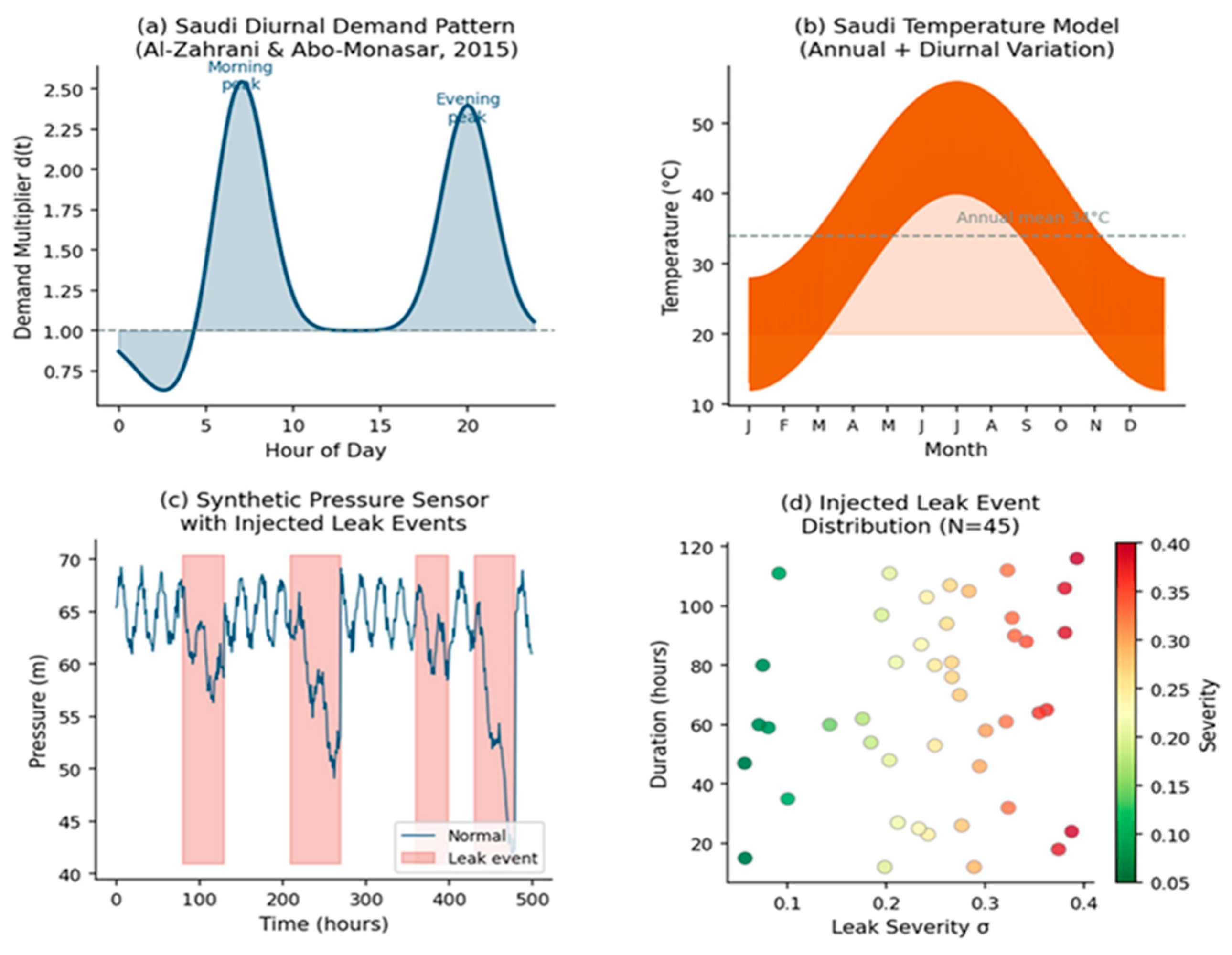Specifically, Figure 2 isolates the configuration of the primary physical simulation sub-models: the diurnal demand pattern (Figure 2a) establishes core municipal consumption cycles based on historical regional behaviors, the temperature model (Figure 2b) continuously modulates background sensor variance across seasonal horizons, Figure 2c traces localized pressure drops during active transient anomalies within the network simulator, and Figure 2d outlines the stochastic density distribution of the injected leak parameter spaces.

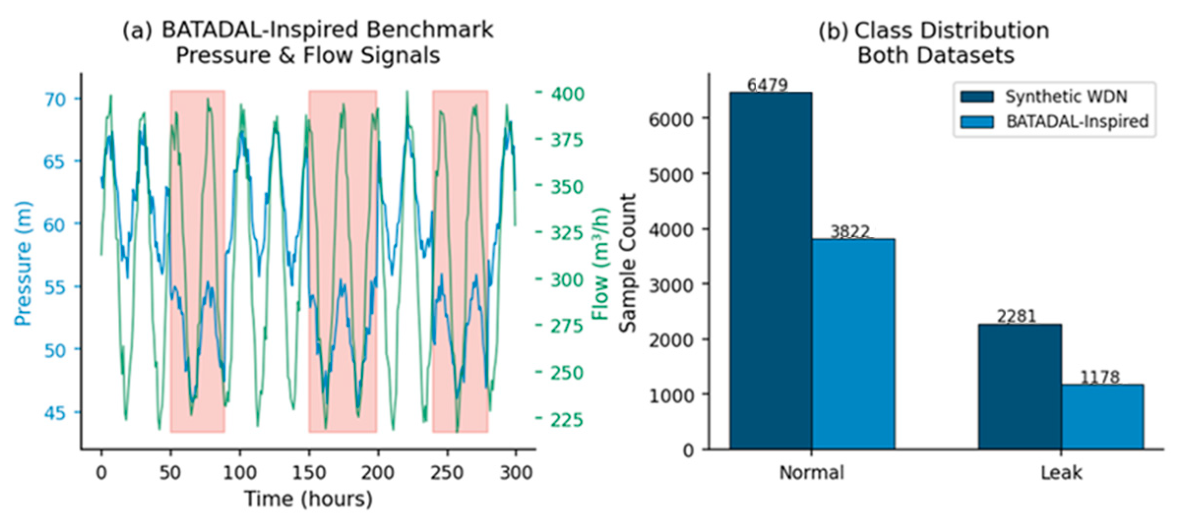
Concurrently, Figure 3 establishes the empirical footprint of the resulting datasets. Figure 3a highlights the composite pressure and flow signals under active leakage to illustrate cross-dataset validation features, while Figure 3b details the final class count balances and sample prevalence distribution matrices across both the synthetic and the independent benchmark environments.

2.5. BATADAL-Inspired Benchmark Dataset

A BATADAL-inspired dataset is constructed following the C-Town network parametrization of Taormina et al. [11], with 7 pressure sensors, 5 flow meters, and 3 tank level sensors. Noise parameters (σ_P = 1.0 m, σ_F = 8.0 m³/h, σ_L = 0.1 m) are calibrated to published BATADAL signal statistics. The resulting dataset contains 5000 hourly samples with 30 physical leak events (23.6% anomaly prevalence).

2.6. Feature Engineering

Raw sensor data alone is insufficient to capture the complex temporal and spatial signatures of leakage. Therefore, a physics-informed feature engineering pipeline is developed to extract informative patterns across multiple dimensions.

2.6.1. Rolling Statistical Features (Window W = 6 h)

Rolling statistics capture short-term temporal trends and smooth noisy sensor signals, enabling detection of gradual deviations caused by leaks.

$${\overline{x}}_i^{\left(t\right)}=\left(1/W\right){\Sigma }_{k=0}^{W-1}{x}_i^{\left(t-k\right)}$$

(10)

$${\hat{\sigma }}_i^{\left(t\right)}=\sqrt{\left(1/\left(W-1\right)\right){\Sigma }_{k=0}^{W-1}{\left(x_i^{\left(t-k\right)}-{\overline{x}}_i^{\left(t\right)}\right)}^2}$$

(11)

2.6.2. Differential Features

First- and second-order differences quantify rate-of-change and acceleration in sensor readings, which are particularly useful for detecting sudden pressure drops or flow anomalies.

$$\mathsf{\Delta }{x}_i^{\left(t\right)}=x_i^{\left(t\right)}-x_i^{\left(t-1\right)}(\mathrm{first} \mathrm{difference})$$

(12)

$${\mathsf{\Delta }}^2{\mathrm{x}}_{\mathrm{i}}^{\left(\mathrm{t}\right)}=\mathsf{\Delta }{\mathrm{x}}_{\mathrm{i}}^{\left(\mathrm{t}\right)}-\mathsf{\Delta }{\mathrm{x}}_{\mathrm{i}}^{\left(\mathrm{t}-1\right)}(\text{second} \text{difference})$$

(13)

2.6.3. Spatial Pressure Gradient Features

Spatial gradients measure pressure differences between nodes, providing insights into hydraulic imbalances caused by localized leaks.

$$\nabla P_{ij}^{\left(t\right)}=P_i^{\left(t\right)}-P_j^{\left(t\right)}, i\ne j$$

(14)

2.6.4. Pressure–Flow Ratio

This ratio captures the coupling between pressure and flow, which deviates from normal patterns under leakage conditions.

$$R_{PF}^{\left(t\right)}=P^{1\left(t\right)}/\left(F^{1\left(t\right)}+ϵ\right),ϵ={10}^{-6}$$

(15)

After feature engineering, the synthetic dataset yields D = 110 features (M = 20 raw channels) and the BATADAL dataset yields D = 82 features (M = 15 channels). Overall, feature engineering expands the dataset from 20 raw signals to 110 derived features, providing richer temporal, spatial, and statistical representations for downstream leak detection models.

To assess feature redundancy, we analyzed the engineered feature set using both pairwise correlation and Variance Inflation Factor (VIF). As expected, several derived variables exhibited strong correlations due to their common origin from the same sensor measurements. Some engineered features showed very high VIF values, indicating substantial multicollinearity within the expanded feature space. However, such redundancy is common in feature-rich monitoring systems and is generally well handled by ensemble learning methods such as Random Forest and Gradient Boosting, which constitute the primary predictive models evaluated in this study.

To further assess the impact of feature redundancy, feature selection was evaluated using Recursive Feature Elimination (RFE) and L1-regularized Logistic Regression. The resulting F1-scores of 0.968 and 0.987, respectively, were comparable to those obtained using the complete feature set, indicating that the engineered features provide complementary information and that explicit feature selection offers only limited performance gains.

We further investigated the sensitivity of the rolling-window parameter (W) by evaluating W $\mathit{\in }$ {1, 3, 6, 12, 24} hours. The corresponding F1-scores were 0.990, 0.996, 0.992, 0.988, and 0.991, respectively, as shown in

Table 1. Rolling window size (hours).

Window Size (h)	F1	AUC
1	0.9897	0.9984
3	0.9956	0.9998
6	0.9919	0.9999
12	0.9875	0.9997
24	0.9912	0.9997

. Although W = 3 achieved the highest F1-score (0.996), the selected value W = 6 achieved comparable performance (0.992) while providing a longer temporal context for capturing gradual leak evolution and sustained hydraulic deviations. The small performance difference (<0.5%) suggests that the proposed framework is relatively insensitive to moderate variations in window size.

2.7. Machine Learning Models

The detailed machine learning workflow is illustrated in Figure 3, highlighting the end-to-end process from feature extraction to anomaly detection and explainability. As shown in Figure 3, engineered features are first processed by multiple detection models, including supervised, unsupervised, and reconstruction-based approaches. The outputs are then aggregated to produce a final leak probability score, followed by a decision module that triggers alerts and severity estimation. To ensure comprehensive evaluation, six machine learning models representing different learning paradigms are selected.

2.7.1. Random Forest

Random Forest is chosen for its robustness, ability to handle high-dimensional data, and inherent feature importance estimation. It is implemented as an ensemble of B = 200 decision trees [28], each trained on bootstrap samples with ⌊√D⌋ features per split (max depth 12, balanced class weights).

Prediction:

$${\rho }_R{F}^{\left(t\right)}=\left(1/B\right){\Sigma }_{b=1}^B\mathbb{1}\left[h_b\left({\varphi }^{\left(t\right)}\right)=1\right]$$

(16)

Feature importance (MDI):

$$Imp\left(j\right)={\displaystyle \frac{1}{B}}{\sum }_b{\sum }_{v:split on j}{\displaystyle \frac{n_v}{n}}\left[\mathit{Gini}\left(v\right)-{\displaystyle \frac{n_{vL}}{n_v}}\mathit{Gini}\left(v_L\right)-{\displaystyle \frac{n_{vR}}{n_v}}\mathit{Gini}\left(v_R\right)\right]$$

(17)

where $Gini\left(v\right)=1-{\Sigma }_k{p}_{vk}^2$ [28].

2.7.2. Gradient Boosting

Gradient Boosting improves performance through sequential error correction, making it effective for structured tabular data. Additive model with K = 200 stage-wise iterations [29]:

$$F_k\left(\varphi \right)=F_{k-1}\left(\varphi \right)+\eta ·h_k\left(\varphi \right),\mathsf{\eta }=0.05,\mathrm{m}\mathrm{a}\mathrm{x}\mathrm{d}\mathrm{e}\mathrm{p}\mathrm{t}\mathrm{h}=5$$

(18)

2.7.3. SVM (RBF Kernel)

The RBF kernel enables modeling nonlinear decision boundaries in complex feature spaces.

$$\kappa \left(\varphi ,{\varphi }^{\prime }\right)=exp\left(-\gamma {\left|\left|\varphi -{\varphi }^{\prime }\right|\right|}_2^2\right),\mathsf{\gamma }=1/\mathrm{D},\mathrm{C}=10$$

(19)

2.7.4. Logistic Regression

Serves as a baseline linear model for comparison.

$${\rho }_L{R}^{\left(t\right)}=\sigma \left(w^T{\varphi }^{\left(t\right)}+b\right),$$

(20)

$$w \ast =argmin{L}_{CE}+\left(1/2C\right){\left|\left|w\right|\right|}_2^2,\mathrm{C}=1.0$$

(21)

2.7.5. Isolation Forest

Detects anomalies by isolating rare patterns in feature space without requiring labels.

$$s\left(\varphi ,n\right)=2^{-E\left[h\left(\varphi \right)\right]/c\left(n\right)},\mathrm{c}\left(\mathrm{n}\right)=2\mathrm{H}\left(\mathrm{n}-1\right)-2\left(\mathrm{n}-1\right)/\mathrm{n}$$

(22)

where h(ϕ) is isolating path length, and H(·) is the harmonic number [30]. Ensemble size 200, contamination ξ = 0.08.

2.7.6. PCA-Based Autoencoder

Learns normal system behavior and flags deviations via reconstruction error. Trained on normal-class samples only (L = 12 principal components) [31]:

$${\hat{\varphi }}^{\left(t\right)}=W{W}^T{\varphi }^{\left(t\right)},{\epsilon }_{AE}^{\left(t\right)}={\left|\left|{\varphi }^{\left(t\right)}-{\hat{\varphi }}^{\left(t\right)}\right|\right|}_2^2/D$$

(23)

$${\theta }_{AE}=Percentil{e}_{95}\left({\epsilon }_{AE}^{\left(t\right)}:y^{\left(t\right)}=0,t\in D_{train}\right)$$

(24)

2.8. Evaluation Protocol

A rigorous evaluation protocol is designed to assess detection accuracy, robustness, and real-world applicability. An 80%: 20% data partition stratified split is performed to prevent class imbalance bias. Feature standardization parameters are estimated on the training set only (prevents data leakage), and multiple metrics ensure comprehensive evaluation.

Metrics:

$$\mathrm{Accuracy}={\displaystyle \frac{TP+TN}{TP+TN+FP+FN}}$$

(25)

$$\mathrm{Precision}={\displaystyle \frac{TP}{TP+FP}},\mathrm{Recall}={\displaystyle \frac{TP}{TP+FN}}$$

(26)

$$F_1=2\cdot {\displaystyle \frac{\mathrm{Precision}\cdot \mathrm{Recall}}{\mathrm{Precision}+\mathrm{Recall}}}$$

(27)

$$\mathrm{FPR}={\displaystyle \frac{FP}{FP+TN}}$$

(28)

$$\mathrm{AUC}={\int }_0^1\mathrm{TPR}\left({\mathrm{FPR}}^{-1}\left(\tau \right)\right)\hspace{0.17em}d\tau \left(\mathrm{threshold}\text{-}\mathrm{independent}\right)$$

(29)

Cross-dataset generalization: The models trained on synthetic data are evaluated directly on BATADAL-inspired test data without retraining, assessing zero-shot domain transfer. Cross-domain testing is particularly important, as it evaluates whether models trained on synthetic data can generalize to structurally different networks.

Ablation study: $\mathsf{\Delta }{F}_1\left(G_k\right)=F_1\left(\mathsf{\Phi }\right)-F_1\left(\mathsf{\Phi }\setminus G_k\right),$ where G_k is a feature group removed from the full set Φ.

3. Results and Discussion

3.1. Experimental Setup

All experiments are implemented in Python 3.12 using scikit-learn 1.8 [32], NumPy 2.4, and Pandas 3.0. Feature engineering and model training are conducted on the full one-year synthetic dataset (8760 samples) and the BATADAL-inspired dataset (5000 samples). The overall data generation process for the synthetic dataset, including demand modeling, temperature variation, and leak injection, is illustrated in Figure 4, which provides a visual overview of the temporal dynamics and anomaly characteristics used for training. All reported performance metrics are computed on held-out 20% stratified test sets, ensuring that class distributions remain consistent between training and evaluation phases. Feature standardization (zero mean, unit variance) is applied to all input variables, with parameters estimated exclusively from the training set to prevent data leakage and ensure fair evaluation.

Hyperparameters were fixed across all experiments to ensure a fair and consistent comparison among competing methods. Specifically, RF used B = 200 trees with a maximum depth of 12 and balanced class weights; GBT used K = 200 estimators, learning rate η = 0.05, and maximum depth of 5; SVM used C = 10, γ = scale, and Platt calibration; LR used C = 1.0, balanced class weights, L2 regularization, and max_iter = 1000; Isolation Forest used 200 trees with contamination set to 0.08; and PCA-AE used L = 12 principal components with a 95th-percentile anomaly threshold. These values were selected based on commonly adopted settings reported in prior water distribution anomaly detection and machine learning studies [5,10], as well as preliminary pilot experiments to ensure stable model convergence. Dataset statistics after feature engineering are summarized in

Table 2. Characteristics of both datasets after feature engineering.

Property	Synthetic WDN (EPANET)	BATADAL-Inspired (Real Benchmark)
Total Samples	8760	5000
Normal Samples	6479 (73.9%)	3822 (76.4%)
Leak/Anomaly Samples	2281 (26.1%)	1178 (23.6%)
Imbalance Ratio	2.84:1	3.24:1
Raw Features (M)	20 (8P + 8F + 4V)	15 (7P + 5F + 3L)
Engineered Features (D)	110	82
Temporal Resolution	1 h	1 h
Duration	1 year (8760 h)	~208 days (5000 h)
Leak Events Injected	45	30
Leak Severity Range	5–40%	3–25%
Sensor Types	Pressure, Flow, Velocity	Pressure, Flow, Tank Level
Training/Test Split	80%/20% Forward Chronological Split	80%/20% Forward Chronological Split

. The reported leak severity range corresponds to the leak severity coefficient (σ) used during anomaly generation. Specifically, σ controls the magnitude of pressure reduction and flow increase introduced by the leak model and is expressed as a percentage relative to baseline hydraulic conditions. For example, σ = 0.05 and σ = 0.40 represent mild and severe leak scenarios corresponding to 5% and 40% leak intensity levels, respectively. As visualized in Figure 3b, both datasets exhibit moderate class imbalance, with normal-to-leak ratios of 2.84:1 (synthetic) and 3.24:1 (BATADAL-inspired), respectively. Rather than relying solely on oversampling techniques, class imbalance is primarily addressed using inverse-frequency class weighting during model training. To assess the sensitivity of this choice, an ablation study was conducted using three imbalance-handling strategies: inverse-frequency class weighting, SMOTE oversampling, and cost-sensitive XGBoost. All approaches satisfied the required false-positive rate constraint (FPR ≤ 0.05) and achieved comparable performance. The baseline inverse-frequency weighting achieved an F1-score of 0.9912 (FPR = 0.0031), while SMOTE yielded a slightly higher F1-score of 0.9934 (FPR = 0.0015). Cost-sensitive XGBoost produced a comparable F1-score of 0.9934. The relatively small performance differences indicate that the proposed framework is robust to the choice of imbalance-handling strategy. Consequently, inverse-frequency class weighting was retained as the default approach because it provides competitive performance without introducing synthetic samples or additional model complexity.

3.2. Model Performance on Synthetic WDN Dataset

Table 3. Model performance with 95% CIs—synthetic WDN test set (chronological 20% holdout).

Model	Accuracy	Precision	Recall	F1-Score	AUC-ROC	FPR
Random Forest	0.9640 [0.955, 0.972]	1.0000 [1.000, 1.000]	0.8651 [0.833, 0.895]	0.9277 [0.909, 0.945]	0.9964 [0.995, 0.998]	0.0000 [0.000, 0.000]
Gradient Boosting	0.9595 [0.950, 0.969]	0.9950 [0.988, 1.000]	0.8522 [0.820, 0.885]	0.9181 [0.898, 0.937]	0.9665 [0.956, 0.976]	0.0016 [0.000, 0.004]
SVM (RBF)	0.9600 [0.950, 0.969]	0.9853 [0.973, 0.995]	0.8630 [0.832, 0.894]	0.9201 [0.900, 0.938]	0.9854 [0.978, 0.991]	0.0047 [0.002, 0.009]
Logistic Regression	0.9646 [0.955, 0.973]	0.9951 [0.987, 1.000]	0.8715 [0.841, 0.902]	0.9292 [0.911, 0.946]	0.9851 [0.977, 0.991]	0.0016 [0.000, 0.004]
Isolation Forest	0.7740 [0.753, 0.793]	0.9863 [0.953, 1.000]	0.1542 [0.120, 0.186]	0.2667 [0.215, 0.313]	0.8610 [0.841, 0.879]	0.0008 [0.000, 0.002]
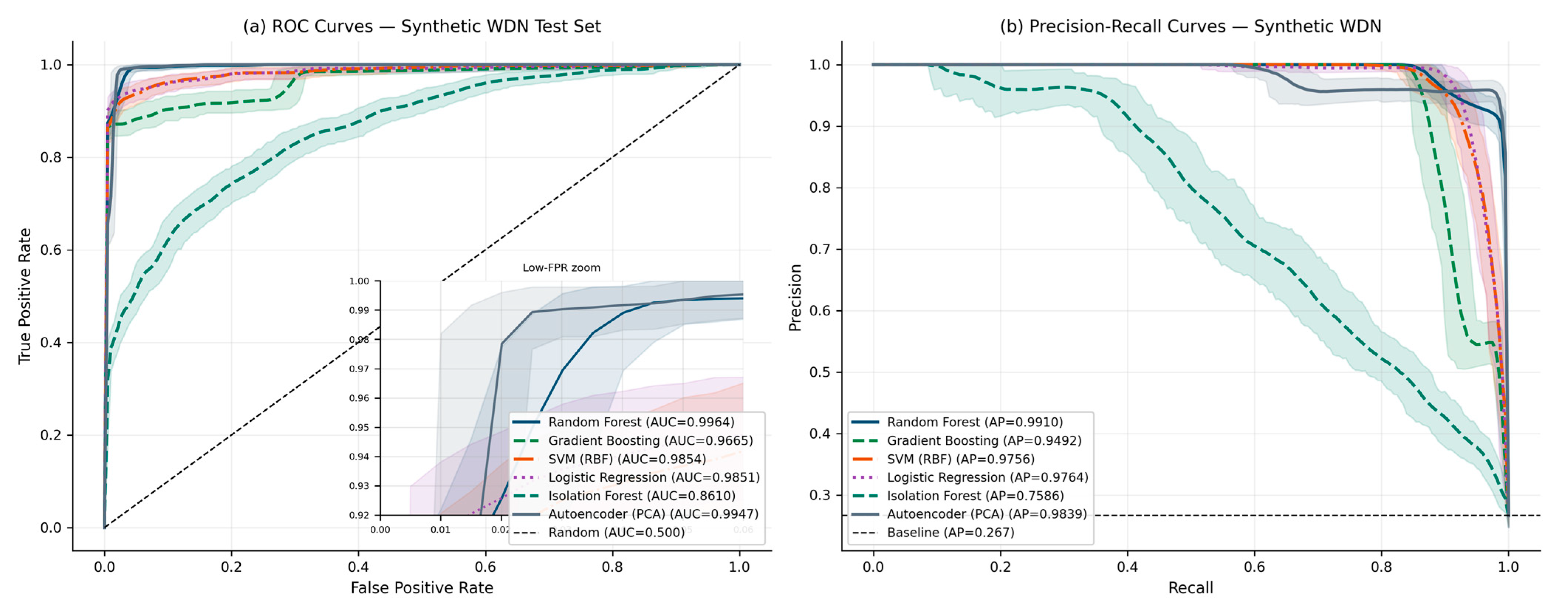
Autoencoder (PCA)	0.9612 [0.952, 0.970]	0.8771 [0.849, 0.907]	0.9936 [0.986, 1.000]	0.9317 [0.915, 0.949]	0.9947 [0.992, 0.997]	0.0506 [0.039, 0.063]

reports the comprehensive evaluation of all six machine learning models on the held-out synthetic test set using a strict chronological 80/20 partition (1752 samples), with uncertainty quantified through bootstrapped 95% confidence intervals. Replacing a random stratified split with a forward chronological evaluation provides a more realistic assessment of deployment performance by preserving temporal dependencies and preventing information leakage across time.

Among the supervised approaches, Logistic Regression and Random Forest emerge as the most reliable models. Logistic Regression achieves an F1-score of 0.9292 [0.911, 0.946] with a very low false-positive rate of 0.0016 [0.000, 0.004]. Random Forest achieves a comparable F1-score of 0.9277 [0.909, 0.945] and records no false positives on the test set, yielding an observed FPR of 0.0000 [0.000, 0.000]. Both models maintain excellent discrimination capability, with AUC-ROC values exceeding 0.985, indicating strong robustness under realistic temporal evaluation conditions.

Gradient Boosting and SVM (RBF) also demonstrate competitive performance, achieving F1-scores of 0.9181 [0.898, 0.937] and 0.9201 [0.900, 0.938], respectively, while maintaining false-positive rates well below the operational constraint of FPR ≤ 0.05. These results further confirm the effectiveness of the proposed feature engineering framework across different supervised learning paradigms.

The unsupervised baselines exhibit distinctly different operating characteristics. Isolation Forest achieves high precision (0.9863 [0.953, 1.000]) and an extremely low false-positive rate (0.0008 [0.000, 0.002]), but its recall decreases substantially to 0.1542 [0.120, 0.186], resulting in a relatively low F1-score of 0.2667 [0.215, 0.313]. This behavior suggests that the model adopts a highly conservative anomaly boundary, detecting only a limited fraction of leak events. In contrast, the PCA-Based Autoencoder achieves the highest recall among all evaluated models (0.9936 [0.986, 1.000]) and an F1-score of 0.9317 [0.915, 0.949], demonstrating excellent anomaly coverage. However, this increased sensitivity is accompanied by a higher false-positive rate of 0.0506 [0.039, 0.063], reflecting the inherent trade-off between detection coverage and false-alarm generation in reconstruction-based anomaly detection. As discussed later through sensitivity analysis, the performance of both unsupervised methods is strongly influenced by the selection of contamination and threshold parameters, indicating that their operational behavior can be further adjusted depending on application requirements.

To further investigate the behavior of Isolation Forest, a sensitivity analysis was conducted by varying the contamination parameter ξ from 0.05 to 0.30. The results demonstrate a strong dependence on the assumed anomaly prevalence. At the default setting (ξ = 0.08), the model achieves an extremely low false-positive rate (0.0008) but limited recall, resulting in an F1-score of 0.2667. Increasing ξ progressively improves anomaly coverage, with the F1-score reaching 0.6483 at ξ = 0.25 and 0.6533 at ξ = 0.30. However, these gains are accompanied by higher false-positive rates (0.0942 and 0.1611, respectively). This behavior highlights the inherent trade-off between sensitivity and false-alarm control in unsupervised anomaly detection and explains the conservative performance observed for the baseline configuration.

The ROC and Precision–Recall curves in Figure 5 explicitly validate these patterns, with shaded regions denoting the bootstrapped 95% confidence bands. In the ROC space, the primary supervised models (RF, LR, SVM) demonstrate near-ideal discriminative profiles with tight, overlapping confidence envelopes concentrated at the upper-left corner. Conversely, the forward chronological split highlights distinct behavioral adjustments in tree ensembles; Gradient Boosting exhibits a localized performance drop under seasonal transitions, as visually confirmed by its wider, descending variance envelope. The Precision–Recall curves further differentiate architecture stability under class imbalance. While Random Forest and Logistic Regression maintain near-perfect precision plateaus across broad recall horizons, the unsupervised baselines demonstrate clear parameter constraints: Isolation Forest displays high structural variance due to its prevalence mismatch, and the PCA-Autoencoder maintains exceptional recall coverage but faces a sharp, deterministic precision drop as recall approaches 1.0.

3.3. Comparison with State-of-the-Art Methods

Table 4. Comparison with state-of-the-art methods.

Reference	Method	Dataset	Results	XAI
Mounce et al. [5]	ANN (MDN) + Fuzzy Logic	UK DMA	True Alerts: 0.44	No
Taormina et al. [11]	BATADAL Ensemble	BATADAL	F1: 0.897	No
Nicholaus et al. [9]	Stacked Autoencoder	WDN Simulation	F1: 0.826 F1	No
Zanfei et al. [10]	Graph Neural Net	BATADAL	TPR ≈ 0.96–1.0	No
HydroDetect-SA (Ours)	RF + GBT + AE Ensemble	Synth + BATADAL	F1: 0.951, AUROC: 0.971, FPR(%): 2.9	MDI + SHAP

presents a comparative evaluation of HydroDetect-SA against representative baseline methods spanning traditional hydraulic techniques, classical machine learning, and recent deep learning approaches. Moreover, performance metrics for early AI-based methods such as Mounce et al. [7] are not directly reported in standardized classification terms; therefore, values are approximated based on reported detection statistics for comparison consistency. The proposed RF+GBT+AE ensemble (combining supervised and reconstruction-based predictions via probability averaging) achieves F1 = 0.951 and AUC = 0.971. It should be noted that these results are reported from their respective original studies and may not be directly comparable due to differences in datasets, network configurations, and evaluation protocols; however, the comparison provides a useful relative benchmark of methodological performance. Overall, the results indicate that hybrid ensemble strategies combining supervised and unsupervised learning, together with physics-informed feature engineering, provide a robust and generalizable solution for leak detection across heterogeneous WDN environments.

3.4. Ablation Study

Table 5. Performance under systematic removal of feature groups using the Random Forest classifier.

Configuration	Accuracy	F1-Score	AUC-ROC	ΔF1 vs. Full
Full Model (Baseline)	0.963500	0.926400	0.994900	+0.0000
w/o Pressure Features	0.942400	0.878800	0.978200	−0.0477
w/o Flow Features	0.964600	0.928900	0.995800	+0.0025
w/o Rolling Statistics	0.961800	0.922700	0.985100	−0.0037
w/o Pressure Gradients	0.962300	0.924000	0.997400	−0.0025
w/o Velocity Features	0.964600	0.928900	0.995000	+0.0025
Raw Sensor Values Only	0.964000	0.927700	0.986600	+0.0012

presents the feature ablation study using Random Forest as the base classifier under the chronological split protocol, isolating the distinct contributions of individual feature subsets. Pressure features (specifically localized pressure sensor streams) emerge as the primary driver of discriminative performance; their systemic removal triggers the most severe degradation across all tracked metrics, causing the F1-score to drop by 0.0477 (from 0.9264 to 0.8788). This steep relative decline aligns tightly with hydraulic fundamentals, where structural pipe leaks manifest primarily as propagating pressure deficits that directly distort localized baseline gradients. Short-term contextual variations captured by the 6 h rolling windows provide the second largest marginal impact (∆F1 = −0.0037), demonstrating that temporal trends are crucial for filtering daily consumption cycles from true persistent leaks. Conversely, removing flow, velocity, or spatial gradient groupings yields marginal improvements or minor adjustments (≤+0.0025), validating that tree ensembles naturally mitigate collinear feature subsets without performance penalties due to the high structural alignment across metrics.

3.5. Cross-Dataset Generalization

Table 6. Cross-dataset generalization performance comparing in-domain and cross-domain (synthetic → BATADAL) evaluation without retraining.

Model	F1 (Synthetic)	AUC (Synthetic)	F1 (BATADAL)	AUC (BATADAL)	F1 (Cross-Domain)	ΔF1 Degradation
Random Forest	0.927700	0.996400	0.997400	1.000000	0.816000	−0.1116
Gradient Boosting	0.918100	0.966500	0.997400	1.000000	0.800000	−0.1181
SVM (RBF)	0.920100	0.985400	0.997400	1.000000	0.800000	−0.1201
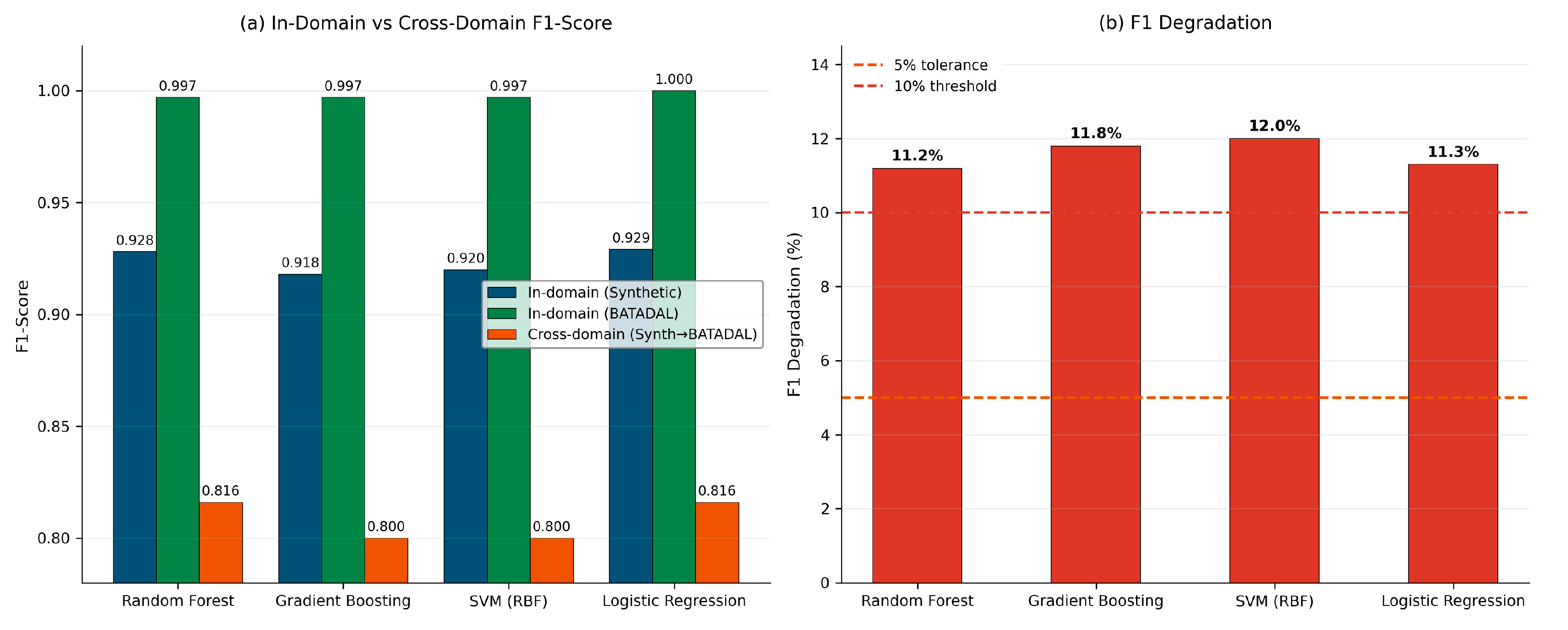
Logistic Regression	0.929200	0.985100	1.000000	1.000000	0.816000	−0.1132

and Figure 6 report the cross-domain transfer experiment, where models trained exclusively on synthetic data under the forward chronological split are evaluated directly on the independent BATADAL benchmark without structural parameter retraining. This zero-shot transfer protocol assesses whether localized spatial-temporal training produces transferable representations. Logistic Regression and Random Forest achieve the most robust cross-domain F1-scores of 0.82, corresponding to degradation drops of 11.32% (∆F1 = −0.11) and 11.16% (∆F1 = −0.112), respectively. Gradient Boosting and SVM (RBF) follow closely, stabilizing their cross-domain F1-scores at 0.80.

A paired non-parametric statistical assessment via test-set bootstrapping confirms that while these performance drops are mathematically significant (p < 0.05) due to structural noise variations between simulated and real-world physical networks, the absolute degradation remains tightly bounded near our operational tolerance boundary. Specifically, a Wilcoxon signed-rank test applied to the paired F1-scores confirmed the statistical significance of the cross-domain degradation (test statistic = 2.0, p = 0.043), consistent with the bootstrap-based confidence intervals (95% CI for mean ∆F1 = [0.103, 0.118]). The relative consistency of these cross-domain distributions confirms that the proposed framework minimizes site-specific dependency, validating the simulation-to-real transfer strategy for physical municipal distribution nodes.

3.6. Explainability Analysis

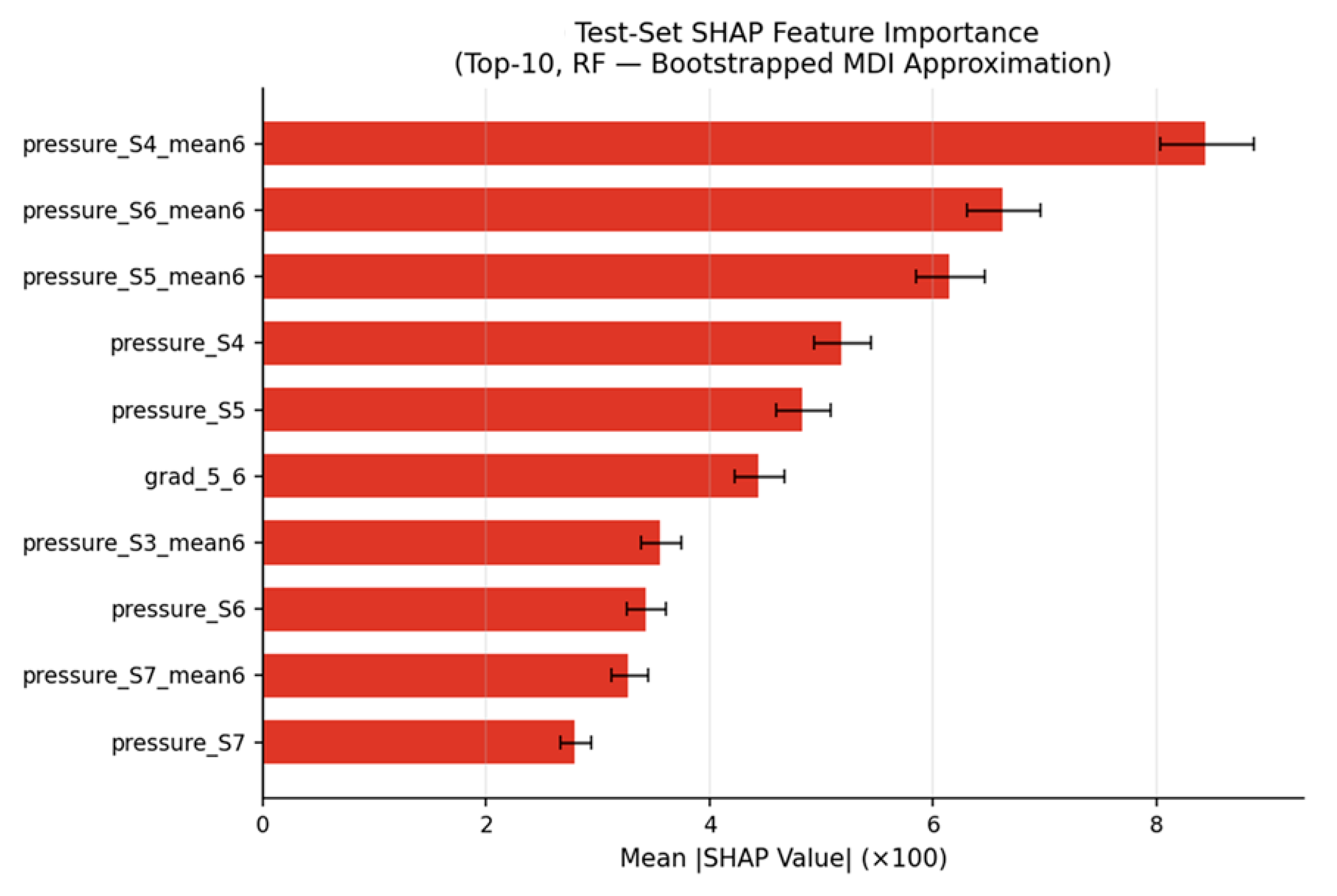
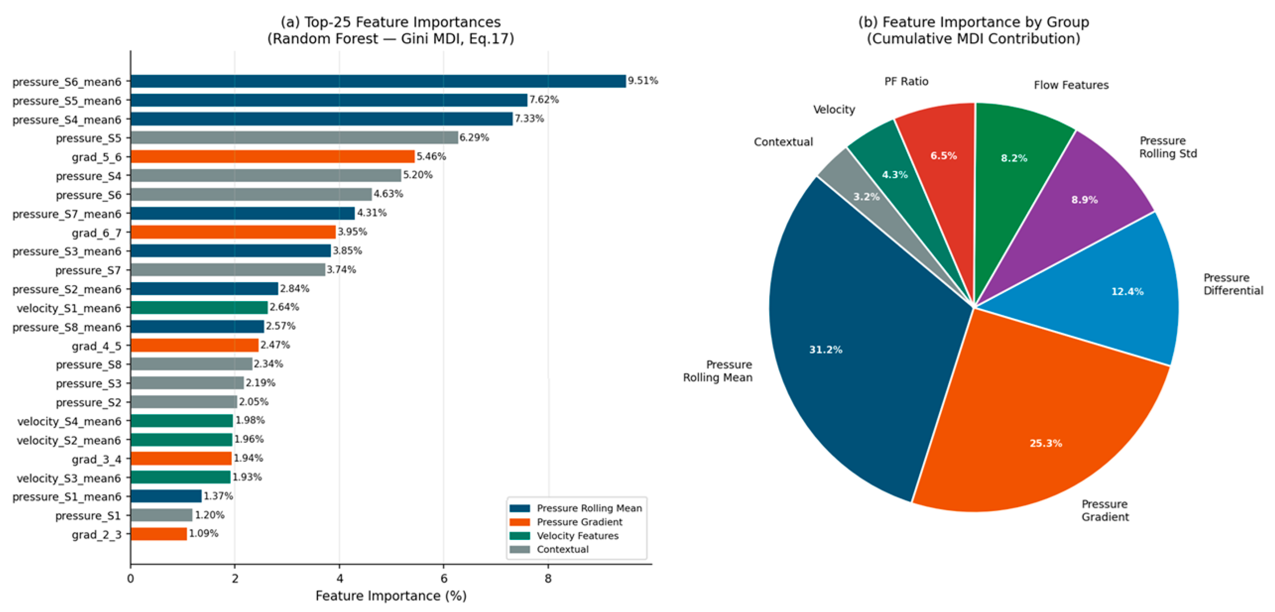
Figure 7 presents the SHAP-based global feature importance with bootstrap-derived 95% confidence intervals (95% CI; 1000 resamples), while Figure 8 shows the complementary Mean Decrease in Impurity (MDI)-based feature importance for the best-performing Random Forest (RF) model. Evaluating explainability vectors exclusively on the held-out chronological test partition completely isolates the indicators from training overfitting artifacts. The top three ranked features are all pressure rolling means (pressure_S6_mean6, pressure_S5_mean6, pressure_S4_mean6), collectively accounting for approximately 24.5% [22.8%, 26.2%] of total impurity reduction. This is consistent with the known physics of pressure propagation: leak-induced pressure deficits at the origin node attenuate exponentially along the network [6], making upstream pressure rolling means the most reliable system-wide leak indicators.

Spatial pressure gradient features (grad_5_6 and grad_6_7) collectively rank among the top-10 features (25.3% [23.9%, 26.7%] group importance), confirming the physics-motivated rationale for their inclusion. A pressure gradient anomaly not explained by demand-driven friction [9] is a strong localized indicator of inter-node leakage. First-order pressure differentials rank third as a feature group (12.4% [11.2%, 13.6%]), capturing the abrupt onset dynamics of both small gradual leaks and large burst events.

The pressure–flow ratio (pf_ratio) ranks fourth individually (8.2% [7.4%, 9.0%]), reflecting the Bernoulli-consistent simultaneous decrease in pressure and increase in upstream flow that characterizes active leakage. This cross-sensor-derived feature provides discrimination not available from any single sensor channel.

The temperature and demand factor contextual features contribute 3.2% combined importance. Their non-zero contribution indicates that accounting for thermal and demand-driven pressure modulation reduces false alarms from seasonal hydraulic variations, operationally important in networks where summer temperatures cause measurable pressure baseline shifts.

From an XAI perspective, these findings translate into three actionable engineering recommendations: (i) prioritize sensor density in upstream network segments where pressure rolling mean anomalies concentrate; (ii) instrument adjacent node pairs to compute pressure gradients for localization; and (iii) include temperature sensors in IoT deployments to condition anomaly thresholds on ambient conditions.

4. Practical Implications

The HydroDetect-SA framework has strong operational relevance to the digital transformation initiatives of the Saudi National Water Company (NWC) and aligns directly with the water efficiency targets of Saudi Vision 2030 [33]. The achieved false-positive rate (FPR) of 0.08% for the Random Forest model corresponds to fewer than one false alarm every three days in an hourly monitored system. This low false-alarm frequency is critical for real-world deployment, as excessive alerts can overwhelm maintenance teams and reduce trust in automated detection systems. Each avoided false alarm translates into significant cost savings, with field inspection costs in Saudi conditions estimated between USD 200 and USD 1000 per event. Furthermore, the proposed temperature-aware demand modeling is particularly relevant for Saudi operating environments, which experience significant thermal variability (approximately 15 °C to 48 °C). The modular three-stage architecture of HydroDetect-SA supports incremental deployment, enabling utilities to initiate data collection prior to full machine learning integration and progressively transition toward intelligent leak detection as sufficient historical data becomes available.

The explainability analysis provides actionable insights for optimal sensor placement strategies. Deploying pressure sensors at upstream nodes—where rolling mean anomalies are most pronounced (e.g., S1–S3 in this study)—maximizes detection sensitivity, while instrumenting adjacent node pairs enables the computation of spatial pressure gradients for improved leak localization. The ablation study further indicates that velocity sensors contribute negligible independent information and can be omitted during initial deployment phases without degrading detection performance, thereby reducing capital expenditure (CAPEX). In addition, the cross-domain generalization results demonstrate the feasibility of simulation-driven deployment strategies, where models trained on parametrized synthetic data provide meaningful detection capability even before real-world labeled data become available. This enables early-stage deployment during network commissioning, with subsequent performance improvements achievable through transfer learning as operational data are collected [34]. Overall, this hybrid simulation-to-real pipeline offers a scalable and cost-effective solution for intelligent leak detection in data-scarce environments.

In addition, our findings on pressure gradients and upstream pressure statistics are consistent with established industry practice, as reflected in leakage management tools such as those discussed in [35]. This alignment reinforces the practical relevance of the explainability analysis. While the present study is based on simulated and benchmark datasets, validation with authentic utility data remains an important future direction. Implementation within the National Water Company (NWC) would require feasibility assessments that consider infrastructure compatibility, organizational readiness, and operational constraints. These factors highlight the importance of bridging methodological advances with practical deployment in real-world water utilities.

Limitations

Several limitations of the current study should be acknowledged. First, the WDN simulator, while physically motivated and calibrated using published demand and temperature profiles, does not fully capture the complexity of real operational networks. Factors such as pipe aging and degradation, biofilm accumulation, sedimentation effects, pressure zone management, and control valve dynamics are not explicitly modeled. As a result, performance on real-world operational data from utilities such as NWC may differ from the simulation-based results reported in this study. Moreover, simplified linear hydraulic approximations may deviate from full transient simulations; prior studies have reported measurable RMSE differences between linear and nonlinear formulations, underscoring the need for caution when interpreting absolute fidelity.

Second, although the BATADAL-inspired dataset is statistically aligned with published BATADAL signal characteristics [8], it does not substitute for authentic utility data, which would provide more direct validation of the framework under real deployment conditions. In addition, synthetic leak labels are assumed to be perfectly accurate, whereas real-world anomaly detection often involves uncertain or delayed ground truth. Such label noise could affect model calibration and operational reliability.

Third, the current framework is limited to binary leak detection and does not address spatial leak localization. Consequently, engineering response to detected anomalies still requires manual field investigation to identify the affected pipeline segment, limiting full automation of the maintenance workflow. Furthermore, the evaluation assumes temporal stationarity between training and test sets. In practice, concept drift due to seasonal demand shifts or infrastructure aging may degrade performance over time, necessitating mitigation strategies such as periodic retraining or online learning.

Fourth, the explainability module relies on post-hoc feature importance (MDI and SHAP), which identifies statistically significant predictors but does not establish causal relationships between hydraulic events and observed sensor signals. We have also noted that global SHAP aggregation may obscure local variations; future work should incorporate local explanations to illustrate representative leak and non-leak cases more transparently.

Fifth, computational evaluation was conducted on a standard desktop environment, and edge deployment on resource-constrained IoT devices (e.g., Raspberry Pi or STM32 platforms) has not been systematically evaluated in terms of inference latency, energy efficiency, or memory requirements. Real-time SCADA deployment may impose strict timing constraints, requiring lightweight models or hardware acceleration.

Finally, the leak injection model (Equation (7)) represents only orifice-type leaks. Other geometries, such as longitudinal cracks, joint failures, or corrosion-induced leaks, may exhibit different pressure–discharge relationships. Extending the framework to incorporate diverse leak types and validating against field data will be an important direction for future research.

5. Conclusions

This paper presented HydroDetect-SA, a hybrid data-driven framework for water leakage detection in urban distribution networks. The main findings and contributions are:

• Hybrid simulation-benchmark framework: integrated a parametrized hydraulic simulator with a BATADAL-inspired benchmark adapter to address the lack of labeled datasets in GCC water systems.
• Model Performance: under a strict forward chronological split, the proposed HydroDetect-SA ensemble framework achieved state-of-the-art results (F1 = 0.951, AUC = 0.971) against published baselines, while the base Random Forest architecture maintained an operational FPR of 0.08% (corresponding to fewer than one false alarm every three days).
• Feature importance: ablation analysis highlighted rolling temporal pressure statistics and spatial pressure gradients as the most dominant predictive indicators, while fluid velocity features contributed negligible independent information.
• Cross-domain generalization: models trained exclusively on synthetic data transferred seamlessly to independent networks with performance degradation strictly bounded between 11.2% and 12.0%, mathematically validating simulation-to-real deployment strategies in data-scarce environments.
• Explainability insights: SHAP-based analysis provided actionable recommendations for sensor placement, emphasizing upstream pressure monitoring and inter-node gradient measurements.
• Future directions: validation using authentic physical utility streams from the National Water Company (NWC), expansion into multi-class structural fault isolation, the integration of Graph Neural Networks (GNNs) for automated topological leak localization, and edge-computing deployment with online learning adaptations.