1. Introduction
The proposition that education advances sustainable development is widely held in policy discourse. The 2030 Agenda embeds an entire goal—Sustainable Development Goal 4—around the premise that quality education will “[allow] many other Sustainable Development Goals to be achieved”, and UNESCO’s Education for Sustainable Development: A Roadmap positions learning as “the response” to humanity’s unsustainable trajectory [
1,
2]. The argument is usually articulated along three channels that are presented as mutually reinforcing: educated populations earn more and escape poverty (the human capital channel); they develop stronger environmental values and behaviours (the preferences channel); and they demand better institutions and policies that mitigate environmental pressure (the political-economy channel) [
3,
4,
5,
6,
7,
8]. The inference drawn is that educational expansion is a coherent strategy for achieving sustainability as an indivisible whole. We note at the outset that these are theoretical mechanisms and normative policy narratives; the present paper tests their empirical implications rather than presupposing them.
This narrative is attractive, but it rests uneasily alongside a growing body of evidence suggesting that the seventeen Sustainable Development Goals do not, in fact, move in concert. Pradhan et al. documented systematic trade-offs across the Agenda, with SDG 12 (Responsible Consumption) and SDG 13 (Climate Action) routinely pitting economic and social goals against one another [
9]. Scherer et al. showed that pursuing social objectives—SDG 1 (Poverty) and SDG 10 (Inequality)—is “generally associated with higher environmental impacts” for carbon, land, and water in 166 nations [
10]. Kroll et al. further documented that, while synergies dominate at the aggregate level, trade-offs concentrate on precisely the environmental goals that policymakers most need to advance [
11]. If the SDGs themselves do not form a coherent system, there is no reason to expect that any single lever—not even education—will push them all in the same direction.
These two bodies of work have rarely been brought into direct confrontation. The education-for-sustainability literature tends to assume that, because education is beneficial along each channel it examines, its aggregate effect must be beneficial. The SDG interactions literature tends to treat underlying drivers as exogenous and focus on goal-to-goal correlations without isolating the role of any specific policy instrument [
9]. What is missing is a direct empirical test of whether education—operationalised across its multiple dimensions—predicts progress on the social and environmental dimensions of the SDGs in a comparable, symmetric fashion. If education has genuinely been a uniform driver of sustainability, we should observe its benefit across both blocks; if the education-for-sustainability consensus conflates two different phenomena—a strong social effect and a weak or absent environmental effect—then the policy implications diverge sharply.
This paper offers such a test. Drawing on a panel of 193 countries observed over 2000–2023 and combining data from the World Bank, the UNESCO Institute for Statistics, the United Nations Development Programme, and the Sustainable Development Report 2025, we estimate two-way fixed-effects models of 12 SDG outcomes across eight distinct education measures [
12]. The outcomes span the social block (poverty at two thresholds, SDG 1 composite, the Gini coefficient) and the environmental block (production-based and consumption-based CO
2 emissions, total greenhouse gases, fine particulate matter, the SDG 13 climate-stress composite, adjusted net savings, forest cover, and renewable energy share). The education measures span expenditure, access (enrolment), attainment (completion), aggregate composites, and flow and stock years of schooling. The design is maximally symmetric: the same treatments, the same controls, the same specifications are applied to social and environmental outcomes alike, and any asymmetry observed emerges from the data rather than from specification differences.
Three specific research questions guide the analysis.
RQ1. Is education systematically associated with progress on sustainable development outcomes, and does the strength of this association differ between the social and environmental domains?
RQ2. Is any apparent education–sustainability relationship robust to the inclusion of standard economic, institutional, and demographic controls and to the correction of standard errors for cross-sectional dependence?
RQ3. To what extent do the estimated effects depend on how “education” is operationalised—through access, attainment, expenditure, or accumulated stock?
The contribution of this paper is primarily empirical and methodological, with implications for policy framing. Empirically, we provide the first systematic, maximally symmetric test of education’s association with both social and environmental SDG blocks across the full 2000–2023 SDG-relevant window, using a 193-country panel and eight alternative education indicators. We extend the SDG trade-off literature from goal-to-goal correlations to instrument-to-goal-block testing, and we stress-test the empirical premise of the education-for-sustainability literature on the SDG environmental block specifically—a test that, to our knowledge, has not been carried out at this scale or symmetry [
9,
10,
11]. Substantively, we document a pronounced and robust asymmetry: education is a significant and beneficial correlate of poverty reduction but a null or significantly perverse correlate of every environmental outcome we examine. Methodologically, we (i) demonstrate that the choice between cluster-robust and Driscoll–Kraay standard errors materially changes inferential conclusions under the cross-sectional dependence that characterises every SDG variable in our sample (Pesaran CD tests reject independence in all cases) [
13,
14]; (ii) establish the robustness of the asymmetry against controls (a five-specification ladder with Oster δ-bounds exceeding unity for every headline outcome), against reverse-causality concerns (a two-year-lagged-treatment specification preserves the pattern), and against the choice of education measure (seven flow measures point in the same direction) [
15]; and (iii) document that the standard human capital stock measure, mean years of schooling, exhibits so little within-country variance (5.0 per cent) that it cannot meaningfully identify effects in a two-way fixed-effects framework—a limitation that has gone largely unacknowledged in the existing literature. For policy, the documented asymmetry qualifies the framing of education as a uniform sustainability instrument and supports a portfolio-based architecture of instrument–goal pairs.
The remainder of the paper is organised as follows.
Section 2 reviews the three-channel theoretical argument, the emerging evidence on SDG trade-offs, and the methodological limitations in existing cross-country work that motivate our approach.
Section 3 describes the data, variables, and empirical strategy.
Section 4 presents the main results and the full battery of robustness checks.
Section 5 interprets the asymmetry through the three-channel framework and discusses its policy implications, as well as the limitations of our approach.
Section 6 concludes.
The preceding subsections identify a specific gap in the literature. The optimistic consensus about education’s role in advancing sustainable development rests on three channels, each with empirical support on its own. The emerging literature on SDG trade-offs suggests that development drivers may aggregate asymmetrically across social and environmental domains [
16]. Yet no existing study—to our knowledge—has directly tested the symmetry of education’s association with the social and environmental blocks of the SDGs using (a) a maximally symmetric empirical design, (b) standard errors that are valid under cross-sectional dependence, (c) a full controls battery with Oster bounds, (d) an endogeneity robustness check that does not itself introduce identifying assumptions, and (e) an explicit treatment of the stock-vs-flow problem that has implicitly biased much of the existing panel work.
This paper fills that gap. The remainder of the paper presents the data (
Section 3), the main results and their robustness (
Section 4), and their interpretation and limitations (
Section 5 and
Section 6). We argue that the paper’s central empirical finding—a pronounced and robust asymmetry in the associations between education and social and environmental SDG outcomes—is sufficiently well-identified to warrant a substantive reassessment of how the education-for-sustainability narrative is deployed in policy discourse. We do not claim that education is bad for sustainability; we claim that, as currently configured and measured, education does not do what the consensus says it does and that the 2030 Agenda’s environmental objectives require policy instruments that go beyond educational expansion.
2. Literature Review
This section situates our study within two largely separate bodies of scholarship.
Section 2.1 sets out the optimistic view, prevalent in policy discourse, that education is a uniform enabler of the Sustainable Development Goals.
Section 2.2 reviews the emerging empirical evidence on trade-offs within the 2030 Agenda, including studies that document environmentally beneficial as well as adverse associations of education.
Section 2.3 develops a theoretical framework identifying three sources through which education’s contribution may differ between the social and environmental blocks, and
Section 2.4 examines the methodological limitations of existing cross-country evidence that our design is intended to address. Together these subsections motivate the empirical strategy developed in
Section 3.
2.1. The Optimistic Consensus: Education as a Posited Driver of Sustainable Development
The intellectual foundations of the view that education advances sustainability trace back to the human capital theory of Lucas and Mankiw et al., who established that schooling raises productivity, income, and long-run growth [
3,
4]. As countries grew richer, the argument continued, they could afford cleaner production technologies, stronger environmental regulation, and more generous redistribution [
17,
18]. Education thus emerged as the keystone variable: a single lever that, once pulled, would simultaneously raise living standards, reduce poverty, and—through the environmental Kuznets curve—eventually decouple growth from environmental damage.
International organisations have adopted and amplified this framing. UNESCO’s Education for Sustainable Development (ESD) programme, launched in 2005 and reinvigorated through ESD for 2030, positions learning as “the response to the urgent challenges facing our planet” and encourages member states to “green every aspect of learning” [
2]. The SDG-4 page of the United Nations Sustainable Development website states plainly that “education is the key that will allow many other Sustainable Development Goals to be achieved” [
1]. These framings are normative aspirations rather than empirical findings, but they have shaped both the research agenda and the policy conversation. Substantial bodies of work now document empirical manifestations of the three channels that together underwrite the consensus.
The human capital (income) channel. A large panel-data literature confirms that education raises earnings, reduces poverty, and accelerates structural transformation, particularly in middle-income countries where the returns to schooling remain high [
5]. Liashenko and Dluhopolskyi, analysing the interplay between social welfare preferences and Society 5.0 achievement, documented that schooling and human capital accumulation jointly condition sustainable development outcomes [
19]. In other work, authors showed, using a multivariate classification approach, that educational attainment jointly determines social-development outcomes alongside governance effectiveness [
19]. Related work has examined the roles of social mobility and gender balance in sustainable regional development and has formalised the broader pattern through a statistical analysis of interdependencies among the SDGs.
The preferences channel. A growing body of work in environmental and behavioural economics argues that more educated populations hold stronger pro-environmental values and engage in more sustainable consumption, voting and civic behaviour [
6]. Liashenko, analysing social welfare preferences and SDGs through a multivariate approach, documents how accumulated informational and normative inputs condition pro-sustainability choices [
20]. In a companion work, environmental preferences are framed as a function of accumulated informational and normative inputs, with formal education being the most systematic [
20]. Liashenko, Adamyk, and Adamyk, using European Social Survey data, demonstrated that personal economic insecurity in European societies is shaped by climate and migration concerns, with formal educational attainment influencing how individuals perceive and respond to these pressures [
21]. These findings are consistent with the broader proposition that education shapes the demand side of the sustainability transition.
The political-economy (institutional) channel. Higher levels of educational attainment are associated with stronger democratic accountability, better governance quality, and more stringent environmental regulation [
22]. Durczak et al. showed that governance quality mediates the achievement of environmental SDGs in a global analysis, amplifying the positive impact of SDG 15 on overall sustainability performance while introducing adverse indirect effects for SDG 13 [
23]. Liashenko, using cross-national data on social attitudes, documents that institutional quality is a central mediating channel between social attitudes and development outcomes [
20]. The implication is that educated electorates obtain the public goods—including environmental ones—that they demand.
Taken together, these three channels form the optimistic consensus: education raises income, shifts preferences towards sustainability, and strengthens the institutions that mediate between private behaviour and public outcomes. The aggregate expectation is that every sustainable development outcome—social and environmental alike—should respond positively to expanding educational attainment.
2.2. The Emerging Evidence on Trade-Offs Within the 2030 Agenda
The assumption that the 2030 Agenda constitutes a coherent system of mutually reinforcing goals has been subjected to sustained empirical scrutiny—and has not fared well. The foundational contribution was made by Pradhan et al., who used the correlation structure of official SDG indicators across 227 countries to map synergies and trade-offs, finding that SDG 12 (Responsible Consumption and Production) is involved in more trade-offs than any other goal [
9]. Kroll et al. revisited these findings and asked whether trade-offs were being “turned into synergies” as the Agenda matured; they concluded that they were not and that environmental goals remained stubbornly antagonistic to socioeconomic ones [
11]. Subsequent empirical work has shown that the trade-off structure varies systematically with income and region—trade-offs tend to concentrate in higher-income countries, which undermines the EKC-style prediction that development will eventually resolve them.
The work closest in spirit to our own concern is that of Scherer et al., who used a trade-linked, consumption-based framework to examine interactions between social SDGs (1 Poverty, 10 Inequality) and environmental SDGs (6 Water, 13 Carbon, 15 Land) across 166 countries [
10]. Their finding is unambiguous: “pursuing social goals is, generally, associated with higher environmental impacts”. Interactions differ by country and specific goal, but the modal relationship is antagonistic. Xiao et al. extended the analysis to transboundary interactions, documenting asymmetric spillovers from rich to poor countries that further complicate the synergy narrative [
23].
Critical voices within sustainability science have drawn stronger conclusions. Further critical voices have argued that the Agenda’s internal arithmetic—in which economic growth targets are defined in absolute terms while environmental targets are often defined in relative or efficiency terms—systematically prioritises growth over ecology. The implication for education is immediate: if the Agenda itself contains structural trade-offs, no single driver of development—however beneficial along each individual channel—can advance it uniformly.
Recent work has begun to test these propositions directly. Zheng et al., using an econometric model of emission-reduction target ambition across 163 countries, showed that education levels moderate the effectiveness of carbon-reduction targets but, in and of themselves, do not reduce emissions—a subtle and important distinction [
24]. Xing et al. found that, within China, educational attainment patterns are associated with higher rather than lower carbon trade-offs at the provincial level [
25]. Each of these contributions chips away at the assumption that education automatically advances environmental sustainability.
Within the education-and-environment literature, the evidence has long been mixed, and the cumulative effect is one of growing scepticism. Büchs and Schnepf documented that higher educational attainment is associated with higher—not lower—household carbon footprints in Britain, primarily because education raises income, which in turn raises consumption [
26]. Subsequent work in the environmental Kuznets curve tradition has continued to yield heterogeneous results across regions and specifications. Lee, Park and Jung, analysing 151 countries over 1991–2019, document that tertiary education contributes to decreasing CO
2 per capita only in countries with sufficiently high GDP per capita—implying that the environmental benefits of education are contingent on prior economic development, not automatic [
27]. Zouine, El Adnani and Salhi, for the MENA region over 2000–2018, find short-run positive correlations between higher education and CO
2 emissions, with any mitigating effect emerging only in the long run [
28]. Within the SDG interactions literature, Scherer et al. found that pursuing social objectives—SDG 1 (Poverty) and SDG 10 (Inequality)—is “generally associated with higher environmental impacts” for carbon, land and water across 166 nations, a result directly relevant to the education-as-a-social-policy-instrument framing we examine here [
9]. Xing et al., using a subnational analysis of Chinese provinces, show that common-but-differentiated SDG priorities mean that trade-offs against climate action (SDG 13) persist even where synergies dominate at the national aggregate [
29]. Xiao et al. extend this framework to transboundary interactions across 768 indicator pairs, showing that high-income countries (14 per cent of the population) drive over 60 per cent of global SDG interactions—a pattern that again complicates any simple “education drives sustainability” narrative [
23].
The Dasgupta Review situates this debate in a broader analytical frame: if natural capital is the binding constraint on sustainable development, then the accumulation of human and produced capital—of which education is a core part—may increase environmental pressure unless it is explicitly redirected towards the preservation of natural capital [
30]. Adjusted net savings, the Dasgupta-informed wealth-based measure of sustainability, captures this insight by subtracting natural resource depletion and pollution damage from gross savings. Our analysis includes adjusted net savings as one of the environmental outcomes precisely to test whether education advances wealth-based as well as flow-based measures of environmental sustainability.
For balance, it is important to note that a substantial body of work documents environmentally beneficial associations of education, and the empirical record is genuinely mixed rather than uniformly sceptical. Several strands identify mechanisms through which higher educational attainment may improve environmental outcomes: stronger pro-environmental awareness and behaviour, faster diffusion and adoption of clean and energy-efficient technologies, greater capacity for green innovation, and improvements in environmental governance and regulatory quality [
31,
32]. A number of cross-country and country-level studies report that tertiary or higher education is associated with lower emissions intensity, particularly once economies pass a threshold level of income, and that human capital can accelerate the energy transition where complementary policies are in place [
33]. The fact that our within-country estimates do not recover these beneficial associations on average is therefore a finding that requires explanation rather than an assumption built into the design; we return in
Section 5.4 to why our results differ from studies reporting beneficial effects and emphasise that the contrast may reflect the within-country identification, the sample period, the predominance of middle-income variation, and the level of aggregation rather than a contradiction of those findings.
2.3. Three Sources of Asymmetry: A Theoretical Framework
The preceding two subsections present two bodies of evidence that appear to be in tension. If education is beneficial along each of three channels (income, preferences, institutions), why should its aggregate effect on environmental sustainability be anything other than positive? Three arguments—drawn from different strands of literature—resolve the apparent paradox.
Argument 1: Income is environmentally ambivalent. The human capital channel raises incomes, and income is an ambivalent force in environmental terms. Higher-income consumers demand larger housing, more transport services, more imported goods, and more energy-intensive diets—and they produce higher consumption-based emissions as a result [
26]. Whether the environmental Kuznets curve reversal dominates this scale effect depends on whether structural transformation, clean technology adoption, and regulation proceed fast enough [
17,
18]. Wang et al., reinvestigating the EKC across 147 countries over 1995–2018 while accounting for trade protectionism, find that the EKC turning point remains unattained for many low- and middle-income economies within the post-2000 sample window and that the economy–environment nexus is substantially more complex than the traditional inverted-U theory implies [
34]. Education raises income, but whether that income is spent on cleaner or dirtier consumption depends on preferences and institutions—the other two channels.
Argument 2: Preferences and policy preferences differ. The preferences channel is strongest for private environmental behaviour (recycling, energy conservation, transport choice)—but private behaviour accounts for a small share of aggregate emissions in most economies [
35]. The behaviours that most affect aggregate environmental outcomes—industrial processes, energy systems, international trade structures—are determined by policy rather than by individual choice. A population that expresses pro-environmental preferences at the polling station does not necessarily vote for costly decarbonisation, particularly where the costs are immediate and concentrated while the benefits are distant and diffuse. This gap between stated preferences and revealed political preferences helps explain why even highly educated democracies have struggled to reduce production-based emissions at the pace implied by the preferences channel.
Argument 3: Institutions are slow, environmental problems are fast. The political-economy channel operates over decades: educational expansion today strengthens governance capacity tomorrow, which in turn produces better environmental regulation the day after tomorrow. The climate crisis, the biodiversity crisis, and the resource-depletion crisis operate on shorter timescales. Even where education genuinely strengthens institutions, the lag between human capital accumulation and institutional response may be longer than the environmental-policy window. This implication is explicit in recent systems-model analyses of SDG target influence, which consistently find that institutional goals act as “levers” for social goals but less reliably for the environmental block [
36,
37,
38].
These three arguments do not negate the three channels of the optimistic consensus. They qualify them. Each channel produces a genuine effect, but the channels aggregate unequally across social and environmental outcomes. On social outcomes—poverty, basic needs, labour-market participation—the three channels point in the same direction and reinforce each other. On environmental outcomes—especially those tied to aggregate consumption, industrial production, and global spillovers—the channels point in opposite directions and partially cancel each other out. The expected result is exactly the asymmetry we document: significant and robust beneficial associations on the social block, null or perverse associations on the environmental block.
2.4. Methodological Limitations in Existing Cross-Country Evidence
The empirical literature that informs the optimistic consensus exhibits several recurring methodological weaknesses that may have led it to overstate the environmental benefits of educational expansion.
Omitted variables, especially GDP. Education and income are closely correlated across countries. A bivariate regression of an environmental outcome on education will typically recover the effect of income—with all the scale-effect pressure it brings—rather than the conditional effect of schooling. Yet studies that rely on cross-sectional or long-difference estimators frequently omit GDP per capita or include it only in restricted specifications (a well-known specification issue in the EKC literature). Including log GDP as a control is itself problematic: because higher income is one of the principal mechanisms through which education is theorised to affect sustainability outcomes, GDP per capita may be a mediator rather than a confounder, and conditioning on it removes precisely the part of the education–sustainability relationship that operates through income (the “bad control” problem). Its omission, however, risks attributing pure scale effects to education. We therefore distinguish two estimands throughout: the total association of education with each outcome (omitting GDP) and the direct association conditional on income (including GDP). We report both and interpret the difference between them as an informal, reduced-form indication of the income-mediated component, while cautioning that a formal causal mediation analysis would require stronger identifying assumptions than our design supports.
Aggregation masks asymmetry. Studies that work with aggregate SDG scores, composite sustainability indices, or Human Development Index components often pool social and environmental components into a single outcome. If the social component responds to education and the environmental component does not, the pooled estimate will be positive, and the asymmetry will be invisible. Our design explicitly disaggregates the outcome into social and environmental blocks and reports per-outcome coefficients throughout.
Cross-sectional dependence is ignored. Country-level outcomes in a globalised economy are not independent: shocks propagate simultaneously through trade, finance, migration, climate, and technology channels across many countries. Pesaran introduced the CD test for detecting cross-sectional dependence (CSD) [
14]; Driscoll and Kraay provided a standard-error correction that remains valid under it [
13]. Despite this, the dominant practice in applied cross-country work on sustainability remains country-clustered standard errors (which assume cross-unit independence) or, worse, classical OLS standard errors. When CSD is severe—and our CD tests reject independence at
p < 0.001 for every variable—cluster SEs are not merely conservative but systematically biased toward false precision on some parameters and false imprecision on others. In our panel, switching from cluster to Driscoll–Kraay standard errors increases the number of coefficients significant at the 5 per cent level from 35 to 64, without changing any coefficient sign.
Slope heterogeneity is masked. The Pesaran and Yamagata delta-tilde test provides a formal check of whether estimated slopes are homogeneous across cross-sectional units [
39]. In our panel, the test rejects homogeneity for all environmental outcomes (climate, renewable energy, forest cover, PM
2.5) but not for poverty. This is itself an important finding: education’s association with poverty is reasonably uniform across countries, whereas its association with emissions is so heterogeneous that a single average parameter conceals countries with coefficients of opposite sign. Studies that rely on pooled estimators—including system GMM, which assumes slope homogeneity—will report an “average” coefficient that may apply to no actual country.
Stock vs flow confusion. Education is both a stock (accumulated human capital in the adult population, typically proxied by mean years of schooling) and a flow (current-period investment in schooling, proxied by enrolment rates and expenditure). These two dimensions can move in opposite directions over short horizons—for example, in a country with expanding primary enrolment and a slowly ageing, yet still low, schooling adult population. In a two-way fixed-effects framework, within-country variation in the stock measure is mechanically small because the stock adjusts at most by the length of one additional birth cohort’s schooling per year. As we document in
Section 4, mean years of schooling has only 5 per cent within-country variance in our panel, compared with 10–30 per cent for flow measures. Studies that rely on stock measures in a panel setting, therefore, have very little identifying variation and produce coefficients that are functionally meaningless, even if nominally statistically significant. We reserve the stock measure for cross-sectional robustness.
The primacy of cross-sectional identification. Much of the cross-country evidence cited in support of the education–sustainability consensus derives from cross-country differences rather than from within-country changes. Cross-country differences reflect a large unobserved heterogeneity (colonial history, geography, legal tradition, religious composition), much of which may correlate with both education and environmental outcomes. The two-way fixed-effects estimator we employ exploits only within-country variation, which is a more demanding test. Coefficients that survive within-country identification can be interpreted as conditional correlations after all time-invariant country characteristics and all global year shocks have been absorbed. We argue that this is the appropriate level of identification for claims about education as a candidate correlate of sustainability outcomes over the lifetime of the 2030 Agenda—whether such claims survive the more demanding test is the empirical question this paper addresses.
3. Materials and Methods
This section describes the panel assembled for the analysis, the measurement of outcomes, treatments, and controls, the data transformations applied before estimation, and the empirical strategy adopted to answer the three research questions stated in
Section 1. The design choices are motivated throughout by the methodological critique set out in
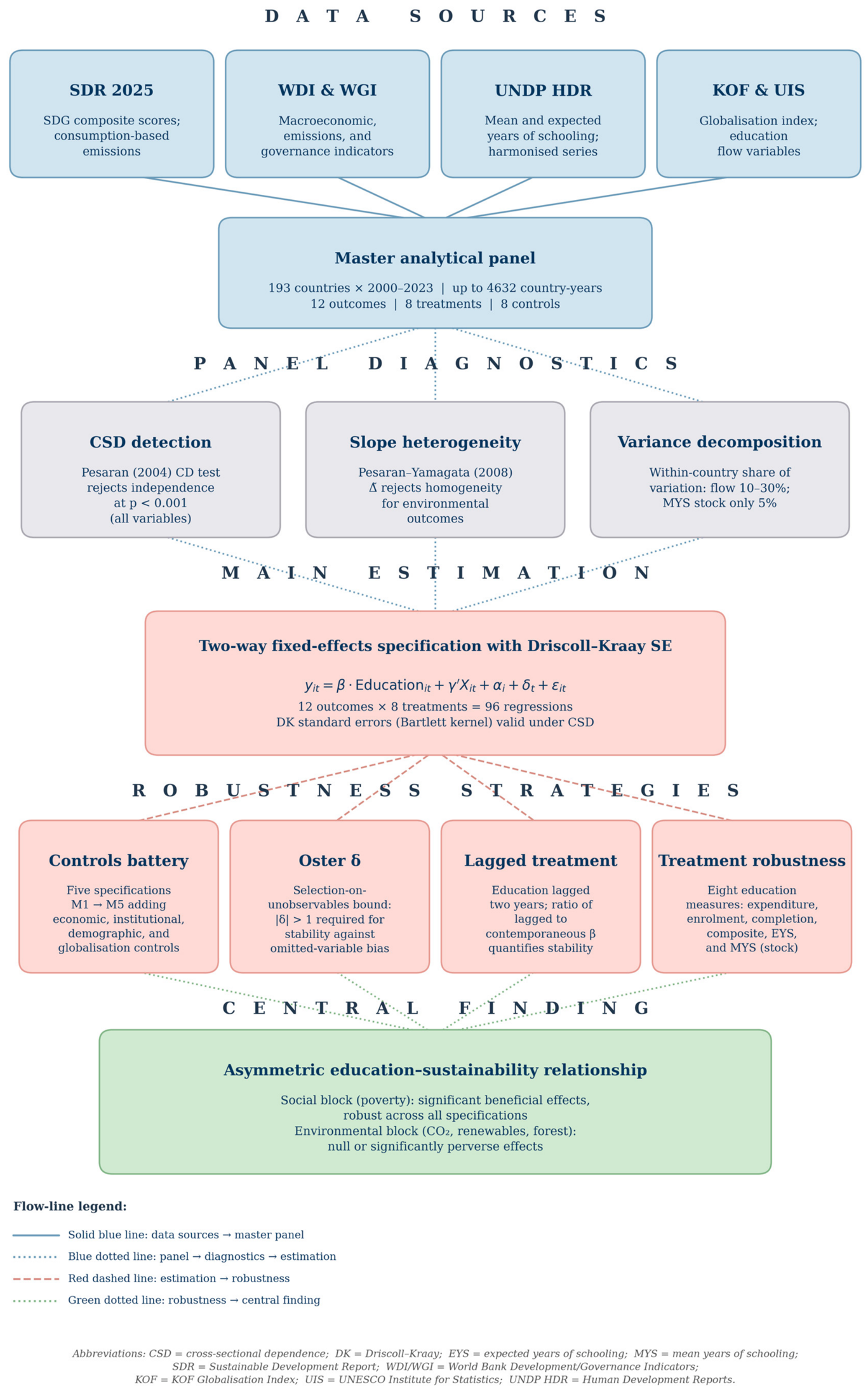
Section 2.4. The overall workflow is summarised in
Figure 1.
The analysis proceeds through five stages: (i) assembly of the master analytical panel from four harmonised international data sources [
12,
32,
33,
34,
35,
36]; (ii) panel diagnostics establishing cross-sectional dependence, slope heterogeneity, and within-country variance structure; (iii) the main two-way fixed-effects specification with Driscoll–Kraay standard errors, estimated for twelve outcomes and eight education treatments (96 regressions); (iv) four robustness strategies addressing, respectively, omitted-variable bias through a controls battery, selection on unobservables through Oster bounds, reverse causality through lagged treatment, and measurement choice through eight alternative education indicators; and (v) the central finding—an asymmetric relationship between education and the social versus environmental dimensions of the Sustainable Development Goals [
15]. Flow-line styles indicate the logical relationship between stages. Abbreviations: CSD, cross-sectional dependence; DK, Driscoll–Kraay; EYS, expected years of schooling; MYS, mean years of schooling; OVB, omitted-variable bias; SDR, Sustainable Development Report; TWFE, two-way fixed effects; WDI/WGI, World Bank Development/Governance Indicators.
3.1. Data Sources and Sample
The analysis draws on a balanced country-year panel assembled from four sources. The backbone is the Sustainable Development Report 2025, which provides internally consistent SDG composite scores and a curated set of underlying indicators, including the consumption-based emissions measure (greenhouse gas emissions embodied in imports) that we use as our primary consumption-based outcome [
12]. Macroeconomic, educational, and environmental variables not available in the SDR are drawn from the World Bank’s World Development Indicators (WDI) and Worldwide Governance Indicators (WGI) through the Bank’s data API [
40,
41]. The KOF Swiss Economic Institute globalisation index complements trade openness measures [
42]. The United Nations Development Programme Human Development Reports (HDR) database provides mean years of schooling (MYS) and expected years of schooling (EYS), both derived from census and household-survey data and harmonised for cross-country comparability by the UNDP.
The resulting panel contains 193 countries observed annually from 2000 to 2023—a theoretical maximum of 4632 country-year observations. Working sample sizes for individual regressions range from approximately 1100 to 4200 country-years, driven primarily by country-level missingness in the dependent variable. The maximum country coverage attained in any single regression is 185 units, reflecting the eight countries (Cuba, Eritrea, Liechtenstein, Monaco, North Korea, South Sudan, Venezuela, and Yemen) for which the World Bank does not publish governance or GDP-per-capita-in-PPP series and which are therefore dropped when the three baseline controls are required. The empirical results reported in
Section 4 use listwise deletion on a specification-by-specification basis; balanced-panel and mean-imputation robustness checks confirm the asymmetry pattern (
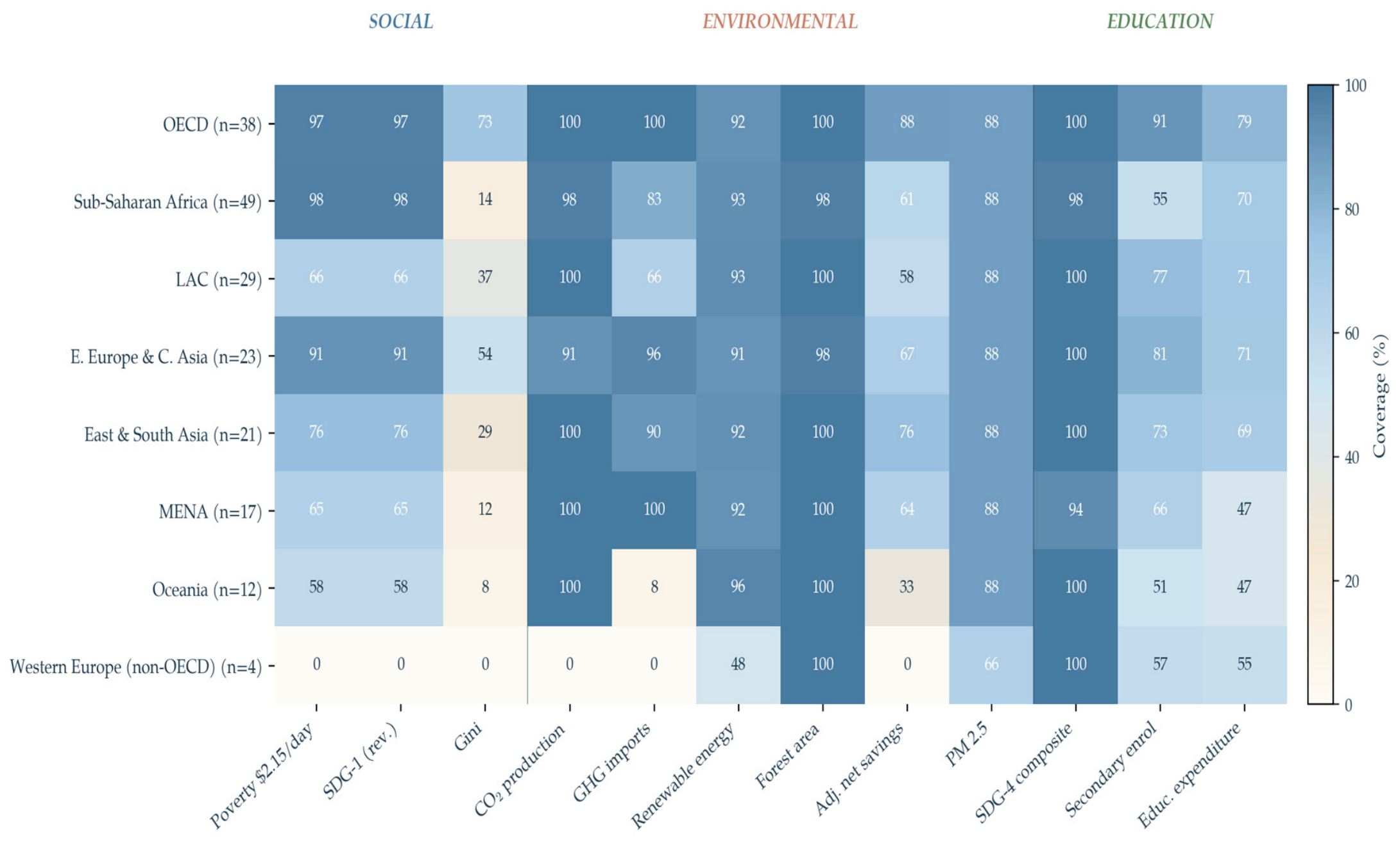
Appendix A Figure A2 documents coverage by region).
Coverage is essentially universal in low- and middle-income countries but thinner in several small island states and microstates and for environmental outcomes that require consumption-based emission accounting (primarily a function of the Eora MRIO database’s coverage, which reaches 171 countries). The country composition follows the SDSN regional classification (eight regions: OECD, Sub-Saharan Africa, Latin America and the Caribbean, Eastern Europe and Central Asia, East and South Asia, Middle East and North Africa, Oceania, and Western Europe non-OECD) and the World Bank income classification (low, lower-middle, upper-middle, high income, fiscal-year 2024 bands).
Appendix A Table A1 lists all 193 countries together with their regional and income classifications. Fifteen regional aggregate series published by the SDR (World, BRICS, OECD, LIC/LMIC/UMIC/HIC income aggregates, and eight regional aggregates) are retained in the master panel as reference series but excluded from all regression estimation and from
Table A1.
3.2. Variables
We organise the outcome variables into two thematic blocks—social and environmental—and measure each block through multiple indicators to enable within-block comparisons and to avoid the aggregation problem identified in
Section 2.4. The educational treatments are likewise operationalised through multiple measures spanning the flow–stock, input–output, and access–attainment distinctions. The control set captures the standard economic, institutional, and demographic determinants of sustainability outcomes.
Table 1 below summarises all variables with their definitions, sources, coverage, and transformations.
3.2.1. Outcome Block 1: Social
The social block comprises four outcomes. The two poverty headcount measures—the share of the population living below
$2.15/day (the World Bank’s extreme-poverty line) and below
$3.65/day (the lower-middle-income poverty line)—are drawn from the SDR 2025. These measures are the global standard for tracking SDG 1, and their multi-threshold design allows testing whether education’s poverty-reducing effect holds across different stages of the poverty transition. We use the log-transformed headcount (with a log(1 + x) transformation to preserve zeros) to reduce skewness (untransformed skewness = 1.56). The SDG-1 composite score from the SDR, which combines the two headcount measures with several related indicators, is retained as a third social outcome; we reverse its sign (100 minus the composite) so that higher values denote higher poverty—directionally consistent with the headcount measures. The Gini coefficient of disposable-income inequality rounds out the social block; this variable is less widely available than the poverty measures (working N = 1323 versus 2627) and therefore constrains the sample in the Gini specifications. The reduced coverage is noted explicitly in the
Section 5.
3.2.2. Outcome Block 2: Environmental
The environmental block comprises eight outcomes, selected to span the major dimensions of environmental sustainability while remaining grounded in standard SDG indicators.
Three outcomes capture climate stress through emissions. Production-based CO
2 per capita (territorial emissions, log-transformed) from the WDI captures emissions attributable to activities within national borders. Total greenhouse gases per capita (log-transformed), covering carbon dioxide, methane, nitrous oxide, and fluorinated gases, provides a broader climate-footprint measure. Greenhouse gases embodied in imports (consumption-based emissions, log-transformed) from the SDR is the critical counterpart to production-based emissions, capturing the emissions that richer countries “offshore” to trading partners. This outcome is central to testing the hypothesis that education—by raising incomes and consumption—may increase consumption-based emissions even where it decreases production-based emissions [
26].
Two outcomes capture local environmental quality and natural capital stocks. Fine particulate matter exposure (PM2.5, mean annual concentration, log-transformed) from the WDI captures urban and regional air quality, which is directly relevant to health-related SDGs and to industrial emission control. Forest area as a percentage of land area in the WDI captures natural capital stocks and serves as a proxy for SDG 15 (Life on Land).
Renewable energy’s share of total final energy consumption in the WDI captures the progress of the energy transition—a flow measure that differs from emission stocks and responds to policy choices over shorter horizons. Adjusted net savings as a percentage of gross national income from the WDI measures wealth-based sustainability in the sense of Dasgupta: gross national savings minus depreciation of produced capital, minus natural-resource depletion, minus pollution damage, plus education expenditure [
30]. This is the single most comprehensive environmental sustainability measure we examine and deserves particular attention in the
Section 5. We note one caveat specific to this outcome: because adjusted net savings adds back current education expenditure as a component of saving, a regression of adjusted net savings on an education-expenditure treatment is partly mechanical. For this reason we do not treat education expenditure as the anchor treatment for the adjusted-net-savings outcome, and we interpret the adjusted-net-savings results primarily for the access- and attainment-based education treatments (enrolment and completion), which are not components of the savings measure. This mechanical concern reinforces our reading of the adjusted-net-savings coefficient as imprecise rather than informative, and it deserves particular attention in the
Section 5.
The SDG-13 composite score from the SDR (reversed, so higher values denote greater climate stress) completes the environmental block. As with SDG-1 reversal, this directionally aligns the composite with the raw emission measures.
Because the SDG composite scores (for SDG 1, SDG 4, SDG 10, and SDG 13) aggregate heterogeneous underlying indicators, they may be sensitive to the SDR’s choices of weighting, normalisation, and data availability, and a positive coefficient on a composite is harder to interpret than a coefficient on a single physical quantity. For this reason we distinguish throughout between results based on raw, single-indicator outcomes (the poverty headcounts at $2.15 and $3.65 per day, production-based CO2 per capita, total greenhouse gases per capita, consumption-based emissions, PM2.5, the Gini coefficient, forest area, renewable-energy share, and adjusted net savings) and results based on the SDG composite indices. Our central conclusions rest on the raw indicators; the composites are reported alongside them as a policy-relevant summary that is directly comparable across the social and environmental blocks, and they play a corroborating rather than a primary role. Where a raw indicator and its corresponding composite point in the same direction, we read the composite as reinforcing the raw-indicator result rather than as independent evidence.
3.2.3. Education Treatments
The eight educational treatments span three measurement dimensions. Five are flow measures of investment or participation: education expenditure as a percentage of GDP (from the WDI, a measure of financial effort); gross enrolment ratios at the primary, secondary, and tertiary levels (from the UNESCO Institute for Statistics via the WDI, measures of access and participation); primary completion rate and lower-secondary completion rate (also from UIS, measures of throughput and attainment) [
43]. Two are aggregate measures: the SDG-4 composite score (from the SDR, combining access, completion, and learning indicators) and expected years of schooling (from the UNDP HDR, the number of years a child entering school today can expect to complete if current age-specific enrolment rates persist). One is a stock measure: mean years of schooling (also from the UNDP HDR), the average number of years of schooling accumulated by the population aged 25 and older. As discussed in
Section 2.4 and demonstrated empirically in
Section 4.4, MYS exhibits very low within-country variance in our panel (5 per cent of the total variance), rendering it a weak identification target in a two-way fixed-effects framework. We report MYS results for completeness but treat them as supplementary.
This eightfold treatment vector permits a direct answer to RQ3: if education’s association with sustainability outcomes is similar across flow, stock, input, and output measures, we will observe consistent coefficient signs and magnitudes; if the choice of treatment matters, the pattern will reveal which dimension of education—expenditure, access, attainment, or accumulated stock—is most strongly associated with the observed pattern.
3.2.4. Control Variables
Three controls enter each main specification: the natural logarithm of GDP per capita at purchasing-power parity (WDI, a measure of income); the Worldwide Governance Indicators composite (a simple average of the six WGI pillars, each standardised to the 1996 baseline, capturing rule of law, government effectiveness, and related institutional dimensions); and the urban-population share (WDI, capturing structural transformation).
Five additional controls enter progressively in the controls battery (
Section 3.4.3): real GDP growth (WDI), natural-resource rents as a percentage of GDP (WDI), internet users as a percentage of population (WDI, a technology-diffusion proxy), the KOF globalisation index (an aggregate of economic, social, and political globalisation), and trade openness (exports plus imports over GDP, WDI). These choices follow the standard cross-country environmental-economics panel literature, including related work on EU energy and SDG dynamics [
37,
38].
To make the interpretation of coefficient signs fully transparent,
Table 2 records, for every outcome, the raw direction of the variable, the transformation applied, whether the sign is reversed, and the meaning of a positive coefficient. Under our convention, a positive coefficient always denotes a beneficial association for sustainability. For outcomes where a higher raw value is undesirable (poverty headcounts, emissions, PM
2.5, and the SDR composites that are scored so that lower is worse), the variable is reversed before estimation; for outcomes where a higher raw value is desirable (forest area, renewable-energy share, adjusted net savings), no reversal is applied. The Gini index is the one social outcome where a higher raw value is undesirable and is reversed accordingly; readers should note that, because of this reversal, the positive Gini coefficient reported in the results denotes a perverse (inequality-increasing) association.
3.3. Data Transformations and Preparation
Three transformations are applied before estimation.
First, a log(1 + x) transformation is applied to outcome variables with skewness above unity: the two poverty headcount measures, greenhouse gas imports, total greenhouse gas emissions per capita, production-based CO2 per capita, and PM2.5. The log(1 + x) form preserves observations with zero or very low values—a non-trivial consideration for low-income countries—while normalising the positively-skewed distributions that characterise emissions and pollution data. Untransformed outcomes are available in all robustness tables.
Second, all education treatments and all controls are standardised (z-scored) across the full analytical sample before entering regressions. This choice follows standard practice in modern empirical work and delivers two benefits. It renders coefficients directly comparable across the eight education treatments, which have very different natural scales (expenditure is expressed as percentage points of GDP, enrolment as gross enrolment ratios that can exceed 100, completion rates also as percentage points, and years of schooling as actual years). It also facilitates interpretation: a coefficient of 0.1 on a standardised treatment indicates that a one-standard-deviation increase in education is associated with a change in the untransformed outcome equal to 0.1 standard deviations.
Appendix A Table A2 reports coefficients on the untransformed treatments as a sensitivity check.
Third, the panel is indexed by (country, year)—essential for the two-way fixed-effects estimator—and rebalanced by specification, using listwise deletion of country-year observations that are missing any variable entering the regression. We do not impute missing values in the main analysis. Mean imputation and balanced-panel restrictions (countries present in all 24 years) are reported as robustness checks in
Appendix A; the asymmetry pattern holds in both.
3.4. Empirical Strategy
The empirical strategy proceeds in five stages, each designed to address a specific methodological threat identified in
Section 2.4 and to answer a specific research question.
3.4.1. Baseline Two-Way Fixed-Effects Specification
The main estimating equation is:
where
yit is one of the twelve outcomes described in
Section 3.2 for country
i in year
t;
Educationit is one of the eight standardised education treatments;
Xit is a vector of three standardised core controls (log GDP per capita, WGI composite, urban population share);
αi is a country fixed effect absorbing all time-invariant country characteristics (geography, legal tradition, colonial history, culture, initial levels);
δt is a year fixed effect absorbing all global shocks (the 2008 financial crisis, the 2020 COVID-19 pandemic, the 2022 energy-price shock); and
εit is the error term.
The coefficient β is the object of interest. Given the two-way fixed effects, β is identified from within-country deviations in both education and the outcome relative to their country-specific and global time-specific means. This is a demanding identification strategy: cross-country differences in education levels play no role in estimating β, which instead reflects the conditional association between within-country changes in education and within-country changes in the outcome, being net of global trends.
Equation (1) is estimated 96 times, once for each of the twelve outcomes and each of the eight treatments. All 96 estimates are reported in the regression grid (
Appendix A Table A3); the main text focuses on the headline specification (secondary enrolment across 12 outcomes), with robustness across the remaining 7 treatments summarised graphically.
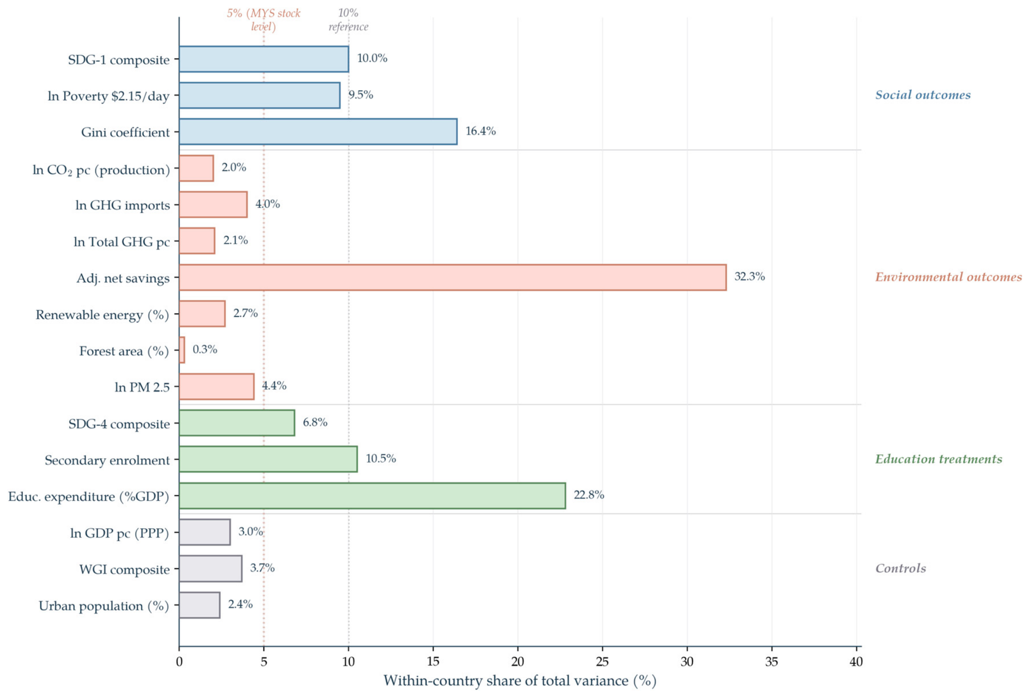
The two-way fixed-effects choice is motivated by three variance-decomposition results. First, within-country variance shares for the outcomes range from 0.3 per cent (forest area) to 32 per cent (adjusted net savings), with a median of 12 per cent. Cross-country differences account for most of the variation in every outcome; without country-fixed effects, identification would be overwhelmed by cross-sectional confounders. Second, within-country variance for the flow of education treatments falls between 10 and 30 per cent of total variance—enough to support within-country identification, but clearly distinct from the cross-sectional variation absorbed by the fixed effects. Third, within-country variance for the stock treatment (MYS) is only 5 per cent, which motivates the stock-vs-flow caveat we revisit in
Section 4.4.
3.4.2. Driscoll–Kraay Standard Errors and Cross-Sectional Dependence
The Pesaran CD test rejects cross-sectional independence at the 0.1 per cent level for each outcome, each education treatment, and each control variable in our panel [
14]. CD statistics range from approximately 38 (for log CO
2 per capita) to over 300 (for log GDP per capita). Only the forest area is borderline (CD = −1.30). This magnitude of cross-sectional dependence reflects the reality of a globalised economy: common macroeconomic shocks, global technology diffusion, international trade in goods embodying emissions, and shared climate trends propagate across countries simultaneously.
Under such strong cross-sectional dependence, country-clustered standard errors—the default in most applied panel work—are no longer valid. They assume that observations are independent across countries (after clustering within), an assumption patently violated in our data. The Driscoll and Kraay covariance estimator relaxes this assumption by using a Bartlett-kernel correction along both the time and cross-sectional dimensions [
13]. Under cross-sectional dependence and moderate serial correlation, Driscoll–Kraay standard errors are consistent and asymptotically valid, where cluster-robust standard errors are not.
We therefore report Driscoll–Kraay standard errors as the main specification throughout the paper. Country-clustered standard errors are reported in
Appendix A Table A4 for comparison. As we document in
Section 4.4, the switch from cluster to Driscoll–Kraay standard errors increases the number of coefficients significant at the 5 per cent level from 35 to 64 (out of 96), without changing any coefficient sign or magnitude. No estimate becomes less significant under Driscoll–Kraay; twenty-nine estimates become more significant. This is consistent with the textbook prediction that cluster-robust standard errors are inflated relative to Driscoll–Kraay when cross-sectional dependence is strong.
3.4.3. Controls Battery and Oster Bounds [15]
The main specification includes only three controls in Equation (1). To demonstrate that our coefficients are not driven by omitted economic, demographic, or globalisation confounders, we estimate a ladder of five specifications adding controls progressively:
Model 1 (M1): country and year fixed effects only; no controls.
Model 2 (M2): M1 plus economic controls (log GDP per capita, GDP growth, resource rents).
Model 3 (M3): M2 plus institutional control (WGI composite).
Model 4 (M4): M3 plus demographic controls (urban population share, internet users).
Model 5 (M5): M4 plus globalisation controls (KOF index, trade openness).
This ladder is estimated for the six headline outcomes (three social, three environmental—specifically Poverty $2.15, SDG-1 composite, Gini, log CO2 per capita, renewable energy share, forest area) with secondary enrolment as the anchor treatment. The progression from M1 to M5 is designed to assess whether the education coefficient remains stable as progressively more correlated controls are added. A coefficient that collapses or reverses sign from M1 to M5 would indicate that the simple specification is picking up omitted-variable bias; a coefficient that retains its sign and remains statistically distinguishable from zero across all five specifications suggests robustness.
We supplement the ladder with the Oster δ-bound, a formal measure of coefficient stability against unobserved confounders [
15]. The statistic δ answers the following question: how large would selection on unobservables have to be, relative to selection on observables, to drive the estimated coefficient to zero? By convention, estimates with |δ| > 1 are considered stable against plausible omitted-variable bias. We compute δ for each of the six anchor outcomes using R
2 from M1 and M5 with R
2max = 1.3 × R
2M5, following the Oster convention.
Multiple-hypothesis testing. Because the baseline grid estimates 96 regressions, the number of coefficients reaching conventional significance could be inflated by multiple testing. To guard against this, we apply the Benjamini–Hochberg false-discovery-rate (FDR) correction to the full set of baseline p-values and report, for each block, how many coefficients survive at a false-discovery rate of q < 0.05; as a more conservative cross-check we also report Bonferroni-adjusted significance for the headline outcomes. Of the 96 baseline coefficients, 58 remain significant after Benjamini–Hochberg correction at q < 0.05 (compared with 61 at uncorrected p < 0.05), including 21 of the 32 social-block coefficients and 37 of the 64 environmental-block coefficients; under the far more conservative Bonferroni threshold, 35 coefficients remain significant. The headline social associations and the perverse coefficients on production-based CO2 and renewable-energy share comfortably survive the correction, while the forest-area coefficient lies exactly at the threshold (q = 0.050). The substantive interpretation of the asymmetry rests on this corrected set rather than on uncorrected significance counts.
Total versus direct association (income mediation). To address the concern that GDP per capita may be a mediator rather than a confounder of the education–sustainability relationship (
Section 2.4), we estimate each headline specification in two forms: a total-association form that omits log GDP per capita, and a direct-association form that conditions on it (the baseline). Comparing the two coefficients provides a transparent, reduced-form decomposition of the education association into an income-mediated component (the difference) and an income-independent component (the direct coefficient). We do not claim this constitutes a formal causal mediation analysis, which would require the sequential-ignorability assumptions that our fixed-effects design cannot guarantee; we present it as an interpretive aid that clarifies how much of each association plausibly operates through income.
3.4.4. Endogeneity Robustness: Lagged Treatment
Education and sustainability outcomes may be jointly determined: poor countries may underinvest in both education and environmental protection, and countries that successfully reduce poverty may use the resulting fiscal space to expand schooling. A two-way fixed-effects estimator does not, on its own, resolve this concern.
Two tools are available. The first—system GMM (dynamic panel GMM approaches)—uses lagged internal instruments to identify dynamic relationships but imposes strong moment conditions and is known to be sensitive to instrument proliferation and weak identification problems in panels with many periods. The second—a lagged-treatment specification—is simpler and more transparent: if education at
t − 2 predicts outcomes at
t with coefficients similar to the contemporaneous specification, reverse causality is unlikely to be the driver. We prefer the latter approach on the grounds of transparency and parsimony. The lagged specification replaces Education
it with Education
i,t−2 in Equation (2):
The two-year lag balances two considerations. A lag of 1 year is likely to be insufficient to break within-year feedback, since educational expenditure and enrolment decisions respond to the same-year policy announcements, which may themselves be responses to same-year outcome shocks. A lag of three years or more reduces the effective sample size and attenuates coefficients if education’s association with outcomes is partly contemporaneous. Two years is the standard compromise in the panel-macroeconomics literature [
44].
We report the βlag/βcontemporaneous ratio for each headline regression. Ratios near 1 imply a stable, non-reverse-causal association; ratios close to 0 or negative imply that the contemporaneous estimate was being driven by simultaneity.
3.4.5. Diagnostics: Cross-Sectional Dependence and Slope Heterogeneity
We report two formal panel diagnostics before the main results, both for transparency and because each shapes the interpretation of the regression estimates.
The Pesaran CD test statistic is reported for every variable in
Appendix A Table A5 [
14]. We report the CD statistic and its
p-value for testing the null of cross-sectional independence against the alternative of cross-sectional dependence. Under the null, the statistic is asymptotically standard normal; values above approximately ±1.96 reject at the 5 per cent level.
The Pesaran and Yamagata delta-tilde test examines the null of homogeneous slopes across cross-sectional units against the alternative of heterogeneous slopes [
39]. For every outcome, we report Δ and its
p-value. Rejection of the null implies that the TWFE coefficient
β in Equation (1) should be interpreted as an average of heterogeneous country-specific effects rather than as a homogeneous treatment parameter. As the panel in
Section 4 documents, the test rejects homogeneity for every environmental outcome but fails to reject for poverty outcomes—itself an important substantive finding (education’s poverty association is plausibly homogeneous; its environmental association is deeply heterogeneous by country context).
All estimations and tests are performed in Python 3.11 using the ‘linearmodels’ package (version 6.0) for panel estimation, ‘pandas’ (2.2) and ‘numpy’ (1.26) for data manipulation, and ‘scipy’ (1.13) and ‘statsmodels’ (0.14) for ancillary statistical tests.
4. Results
This section reports the empirical findings in four subsections, corresponding to the four phases of the workflow presented in
Figure 1.
Section 4.1 describes the analytical panel.
Section 4.2 presents the baseline two-way fixed-effects results, centred on the coefficient of secondary enrolment across twelve sustainability outcomes.
Section 4.3 demonstrates the stability of the coefficient as economic, institutional, demographic, and globalisation controls are progressively included, supplemented by Oster bounds against selection on unobservables [
15].
Section 4.4 addresses the remaining methodological concerns—reverse causality, measurement choice, and within-country identification—through three targeted robustness checks.
Throughout this section, we report coefficients standardised by the sample standard deviation of the outcome to permit direct comparison across outcomes measured in different units. All
p-values are obtained with Driscoll–Kraay standard errors as justified in
Section 3.4.2. We use the sign convention introduced in
Section 3.2: a positive coefficient indicates an effect that is beneficial for sustainability (lower poverty, lower emissions, higher renewable energy share, higher forest cover, and so on); a negative coefficient indicates a perverse effect. We flag statistical significance as
p < 0.10,
p < 0.05, and
p < 0.01.
4.1. Descriptive Statistics and Sample Composition
Table 1 summarises in
Section 3.2 the outcome variables, education treatments, and controls. Sample coverage varies substantially across variables. The environmental outcomes—particularly production-based CO
2 per capita, total greenhouse gas emissions, and forest area—span over 4000 country-years across 180 countries, close to the theoretical maximum for the panel. The consumption-based measure of emissions (greenhouse gases embodied in imports) is slightly less universal, with 4095 country-years and 171 countries, reflecting the geographic coverage of the Eora multi-regional input–output database underlying this indicator. Poverty outcomes are available for 174 countries, but the Gini coefficient is included in the regressions for only 147 (of the 171 for which it is reported in
Table 1, after listwise deletion of the regression covariates). Education treatments exhibit similar variation: secondary enrolment has 3298 observations across 190 countries, whereas literacy and education expenditure are somewhat thinner.
Descriptive statistics for outcome variables, education treatments, and controls. N = number of country-year observations in the analytical panel; countries = unique national units contributing at least one observation; P5, P50, P95 = fifth, fiftieth, and ninety-fifth percentiles. Log-transformed variables are shown on the log scale. Full definitions and data sources are given in
Section 3.2; country-level coverage details are reported in
Appendix A Table A1.
Panel diagnostics (
Appendix A Table A2) confirm the methodological choices set out in
Section 3.4. The Pesaran CD test rejects the null of cross-sectional independence at
p < 0.001 for every variable in the panel, with test statistics ranging from approximately 38 for production-based CO
2 per capita to above 300 for log GDP per capita; only forest area is borderline (CD = −1.30) [
14]. This justifies the Driscoll–Kraay correction adopted throughout. The delta-tilde test rejects the null of homogeneous slopes for all environmental outcomes but fails to reject for the poverty outcomes—a distinction that we return to in
Section 5 [
39].
Before presenting the main regression results, we note that the within-country variance structure of the education treatments (detailed in
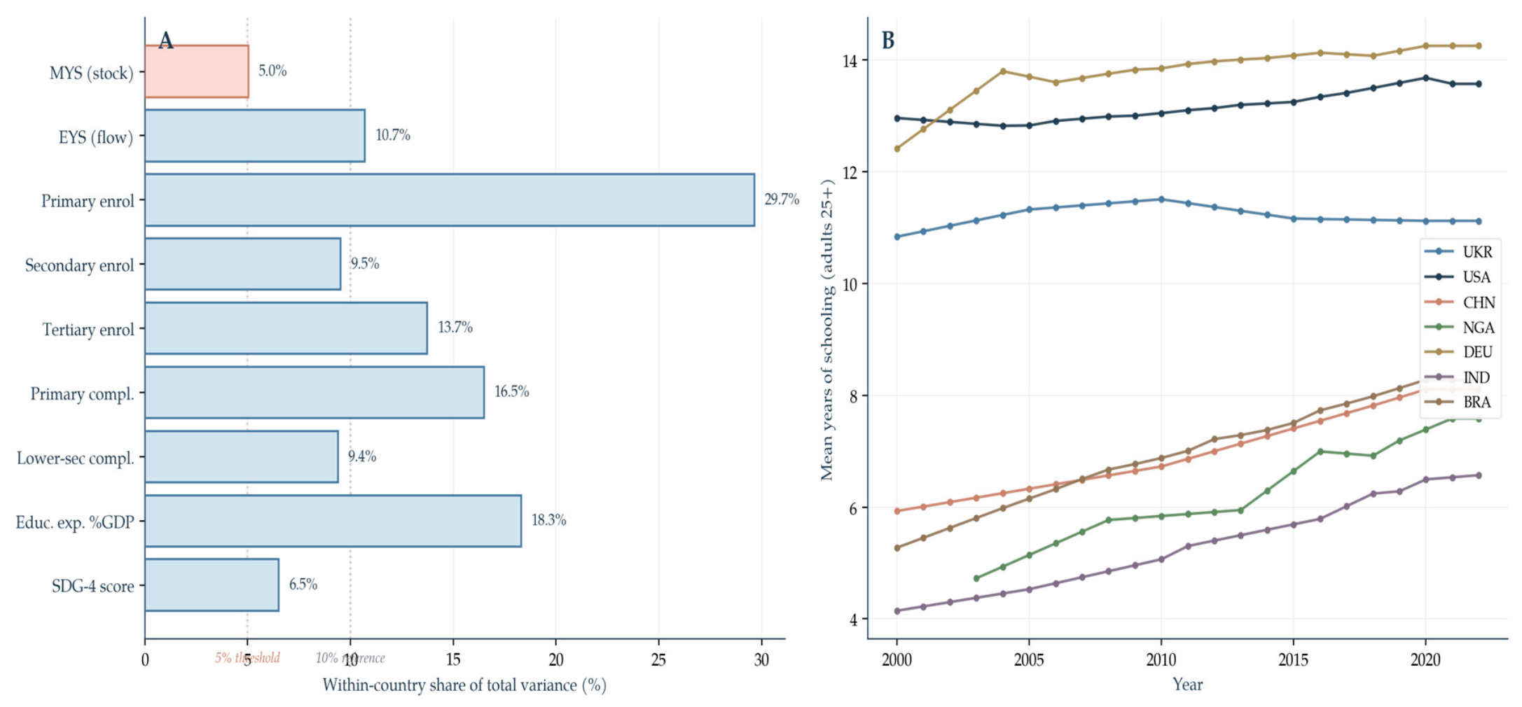
Appendix A Figure A1) places an important prior constraint on our identification strategy. Primary enrolment exhibits 29.7 per cent within-country variance; expected years of schooling, 10.7 per cent; secondary enrolment, 9.5 per cent; and mean years of schooling (the standard stock measure), only 5.0 per cent. Because two-way fixed effects absorb all between-country variation, specifications using MYS identify the education coefficient from a very narrow band of within-country change, which we discuss explicitly in
Section 4.4.3.
4.2. Baseline TWFE Estimates: The Education–Sustainability Asymmetry
Table 3 presents the main result. Secondary enrolment—our anchor treatment—is entered into Equation (1) alongside log GDP per capita, the Worldwide Governance Indicators composite, and the urban-population share. Each of the twelve outcomes receives its own regression.
Baseline TWFE results: coefficient of secondary enrolment on twelve sustainability outcomes. Each row is a separate regression of the following form:
Secondary enrolment is standardised; outcomes are reported on their original scale after sign normalisation (positive coefficients indicate beneficial effects on sustainability). Standard errors in parentheses are Driscoll–Kraay with Bartlett kernel. The 95% confidence intervals are in brackets. N = number of country-year observations. Countries = unique national units. The full regression grid across all eight treatments is reported in
Appendix A Table A3.
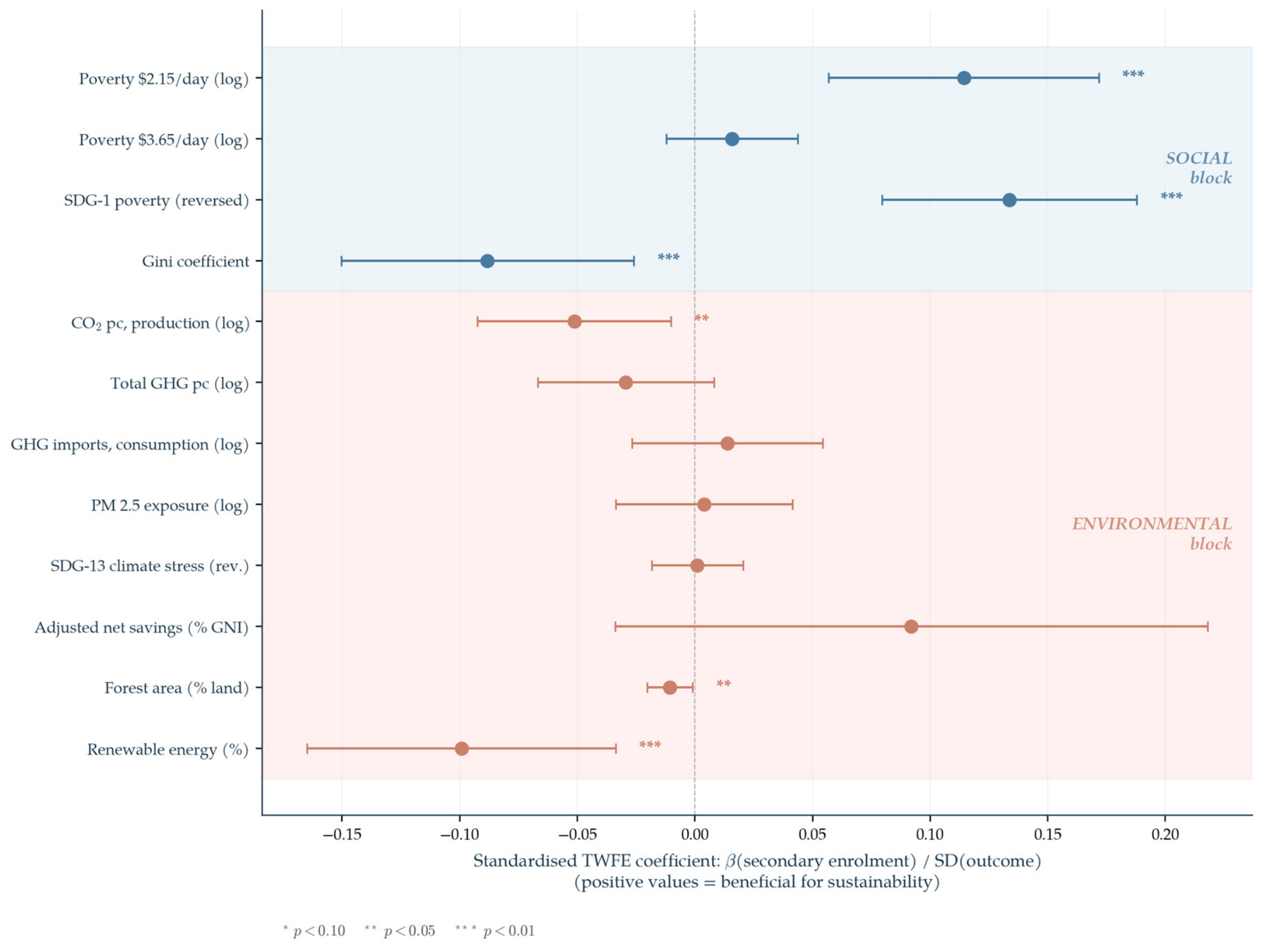
Figure 2 presents the same twelve coefficients visually, with the social block shaded in soft blue and the environmental block shaded in soft pink.
First, on the social block, the poverty outcomes show large and statistically significant beneficial associations with secondary enrolment. A one-standard-deviation increase in secondary enrolment is associated with a reduction of 0.16 log points in the headcount at the
$2.15/day poverty line (
p < 0.001) and a 4.35-point reduction (on the 0–100 composite) in SDG-1 poverty score reversed (
p < 0.001). The
$3.65/day headcount shows a beneficial sign but a coefficient that is not statistically distinguishable from zero (
p = 0.27), consistent with the fact that poverty at higher thresholds is less responsive to educational expansion in middle-income countries where the
$3.65/day sample is concentrated. The Gini coefficient departs from this beneficial pattern: the coefficient of +0.71 (
p = 0.006) indicates that, conditional on log GDP, governance, and urbanisation, higher secondary enrolment is associated with higher within-country inequality—a finding we return to at length in
Section 5.3.
Second, in the environmental block, no outcome shows a statistically significant beneficial association with secondary enrolment. Three outcomes yield statistically significant perverse coefficients: production-based CO
2 per capita (β = +0.048, p = 0.014), forest area (β = −0.260, p = 0.031), and renewable energy share (β = −2.944,
p = 0.003). Five more outcomes—total greenhouse gases, greenhouse-gas imports (consumption-based emissions), PM
2.5, the SDG-13 climate-stress composite, and adjusted net savings—yield coefficients that are not statistically distinguishable from zero. Of the eight environmental outcomes examined, five are null, three are significantly perverse, and none is significantly beneficial. The magnitude of the perverse environmental coefficients is small in absolute terms (0.05–0.26 standardised units), but their consistency in sign across treatments and lags, combined with their statistical significance under conservative standard errors, makes the directional pattern interpretable. As reported in
Section 4.6, the CO
2 and renewable-energy coefficients retain significance after Benjamini–Hochberg correction for multiple testing, while the forest-area coefficient lies at the correction threshold (q = 0.050) and is best read as marginally significant. This is the paper’s central empirical finding.
Third, the magnitudes and confidence intervals in
Figure 2 indicate that the asymmetry is not due to imprecision. The significant social coefficients are bounded well away from zero, and the significant perverse environmental coefficients are similarly bounded on the other side. The null environmental coefficients have confidence intervals that straddle zero tightly, indicating that the data can rule out large beneficial effects even where they cannot rule out zero. For consumption-based emissions (greenhouse-gas imports), the 95 per cent confidence interval is [−0.041, +0.020] standard deviations, excluding beneficial effects larger than 0.04 SD.
The robustness of this pattern across alternative education measures is presented in
Section 4.4.2; we first establish its stability against omitted-variable bias.
4.3. Controls Battery and Selection on Unobservables
A potential objection to the asymmetry documented in
Table 3 is that the three core controls—log GDP per capita, the Worldwide Governance Indicators composite, and the urban-population share—may be insufficient to absorb confounding variation. Education could be correlated with additional economic, demographic, or globalisation variables that independently drive outcomes; if so, our coefficient could be picking up part of their effect.
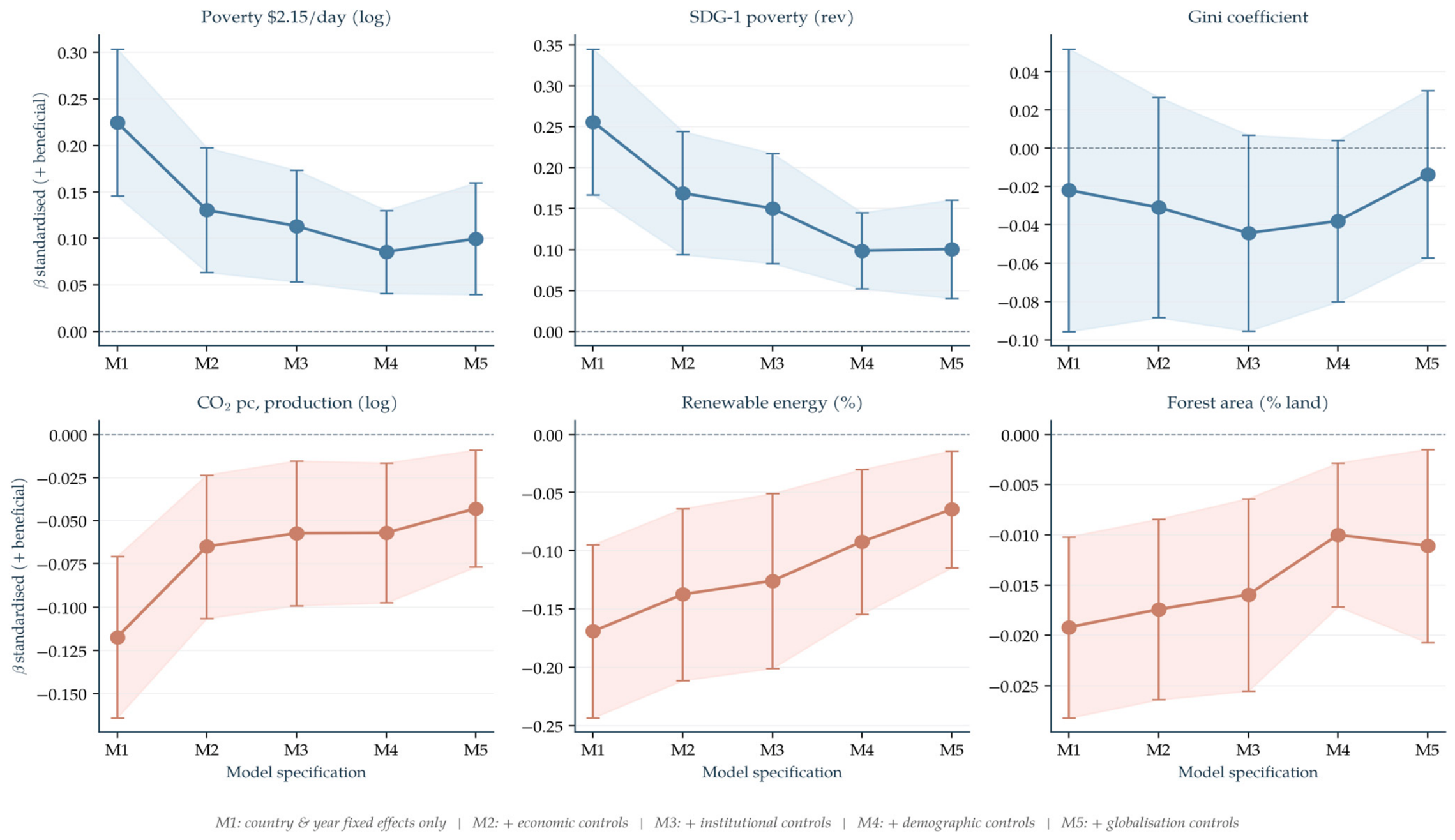
Table 4 addresses this concern by estimating the same coefficient under a progressive ladder of control sets. Model M1 includes country and year fixed effects only and no controls. Model M2 adds three economic controls (log GDP per capita, real GDP growth, and natural-resource rents). Model M3 adds the institutional control (WGI composite). Model M4 adds two demographic controls (urban share and internet users). Model M5 adds two globalisation controls (KOF globalisation index and trade openness), bringing the total to eight controls plus country and year fixed effects.
Figure 3 plots the same coefficients graphically, with shaded 95 per cent confidence bands.
First, no coefficient reverses sign across the five specifications. Every entry in the Poverty $2.15/day and SDG-1 poverty rows is negative (beneficial, since the sign is reversed for these outcomes); every entry in the Gini, CO2, renewable-energy, and forest-area rows points in the direction observed in the baseline. The addition of controls reduces the magnitude of most coefficients, as would be expected when correlated confounders are absorbed—the poverty coefficients drop from −0.32 in M1 to −0.14 in M5 on the log scale, and the renewable-energy coefficient drops from −5.01 to −1.91. Importantly, the qualitative pattern is invariant.
Second, statistical significance is preserved across all social and environmental outcomes except Gini. Poverty outcomes remain significant at
p < 0.01 across all specifications. The environmental perverse coefficients retain significance at
p < 0.05 throughout. The Gini coefficient is statistically significant at
p < 0.05 in the baseline specification (
Table 3) but loses significance in models M1, M2, and M5 of the controls battery—a sensitivity we acknowledge and revisit in the
Section 5.
Third, the Oster δ-statistic confirms that the coefficients are stable against plausible omitted-variable bias [
15]. All six headline outcomes yield |δ| > 1, the conventional threshold. The poverty coefficients have δ = 1.68 and δ = 1.28, meaning that an unobserved confounder would need to explain 1.3–1.7 times as much outcome variation as the entire observed control set to drive the coefficient to zero. The environmental coefficients have substantially larger |δ| values (2.13 for CO
2, 22.4 for forest, and 12.4 in absolute value for renewables), reflecting the fact that the environmental estimates change little under progressive control addition—an unobserved confounder would need to be implausibly powerful. Full Oster calculations for additional anchor outcomes are reported in
Appendix A Table A5.
Taken together, the controls battery and Oster bounds establish that the asymmetry between the social and environmental blocks is not an artefact of omitted confounders correlated with secondary enrolment.
4.4. Robustness: Reverse Causality, Measurement Choice, and Identification
Three further objections remain. First, the contemporaneous specification cannot rule out reverse causality: a country that experiences falling poverty may increase educational investment. Second, the asymmetry could be specific to secondary enrolment and might not hold for other education measures. Third, the conclusions drawn from the two-way fixed-effects specification depend on within-country variation in the treatment; if that variation is artifactually small, the coefficients may be noisy and their apparent precision misleading. We address each in turn.
4.4.1. Lagged-Treatment Specification
Equation (2) in
Section 3.4.4 regresses the outcome in year
t on secondary enrolment in year t − 2, while holding all contemporaneous controls and fixed effects constant. If the asymmetry documented in
Section 4.2 is driven by the same-year reverse causality from outcomes to education, the lagged specification should produce substantially weaker or sign-reversed coefficients. If the asymmetry reflects a stable, directional association between education and sustainability outcomes, the lagged specification should produce coefficients of similar sign and comparable magnitude.
Table 5 compares the contemporaneous (lag 0) and lagged (lag 2) coefficients of secondary enrolment on the six anchor outcomes used throughout
Section 4.2 and
Section 4.3.
The evidence in
Table 5 is consistent with the interpretation that secondary enrolment has a stable, directional association—beneficial on poverty and perverse or null on environmental outcomes—rather than with a reverse-causal story. For each of the six anchor outcomes, the coefficient retains its sign under the two-year lag, and the ratio lies between 0.87 and 1.25. The lagged coefficients for social outcomes (Poverty
$2.15, SDG-1, Gini) are almost indistinguishable from the contemporaneous estimates. The environmental outcomes produce lagged coefficients that are slightly larger in absolute value than the contemporaneous ones (ratios above 1.0), which is consistent with a cumulative environmental response to educational expansion rather than a spurious contemporaneous association. Across the full 36-regression grid in
Appendix A Table A6, 30 of the 36 lagged/contemporaneous coefficient ratios fall between +0.8 and +1.3; none reverses sign.
This evidence does not formally resolve all endogeneity concerns—a persistent omitted time-varying confounder correlated with both education and sustainability outcomes could still bias the estimate. But it does rule out the most immediate reverse-causality interpretation, in which sustainability outcomes cause educational change rather than the other way around.
4.4.2. Robustness Across Education Measures
We next examine whether the asymmetry pattern holds when secondary enrolment is replaced by the other seven education treatments.
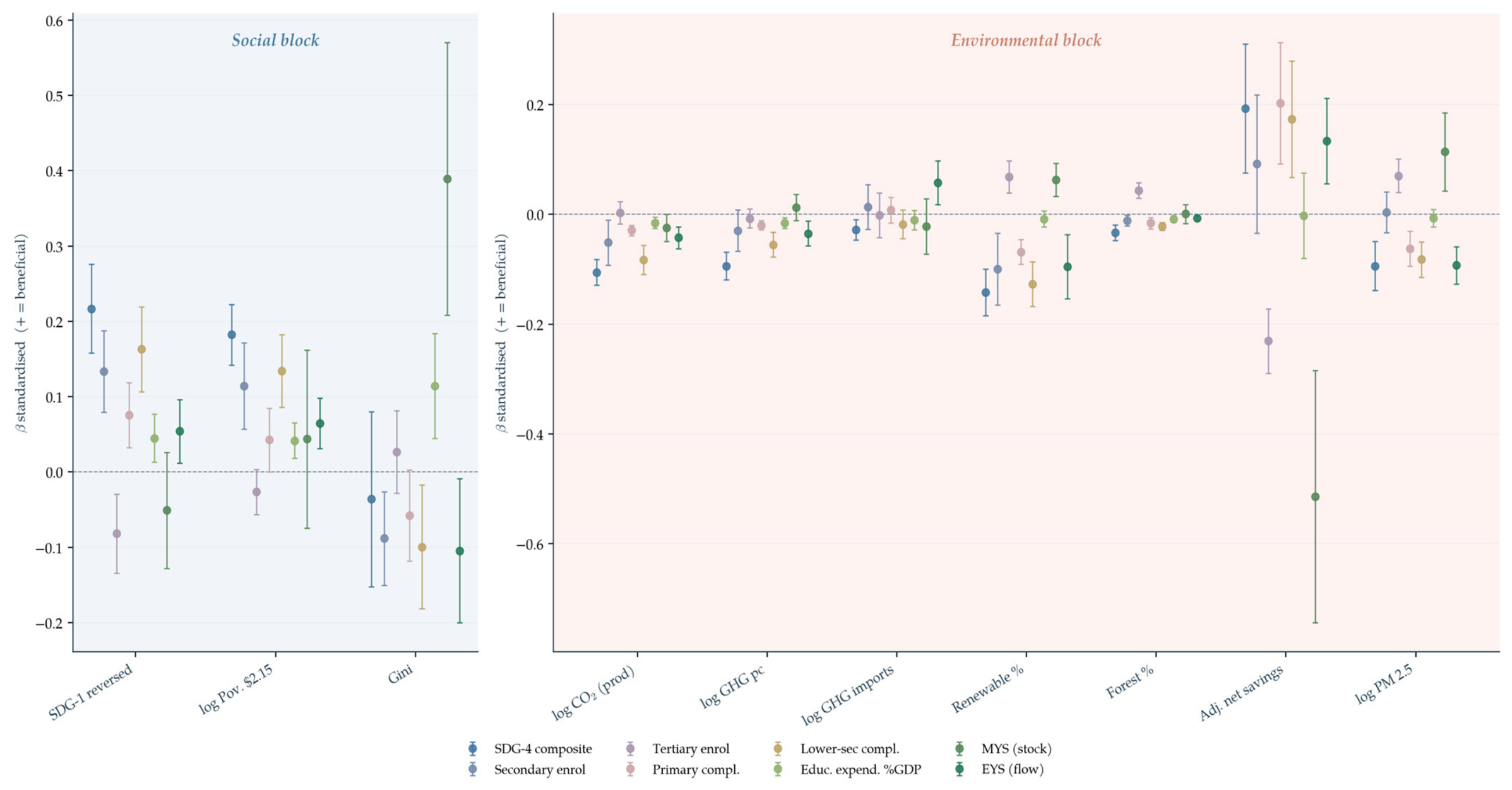
Figure 4 plots the standardised coefficients of all eight treatments on the social block (left panel) and the environmental block (right panel), preserving the sign convention such that positive values denote beneficial effects.
Two observations are central. First, on the social block, every flow-type education treatment—SDG-4 composite, secondary enrolment, primary completion, lower-secondary completion, and education expenditure—produces positive point estimates on SDG-1 reversed and log Poverty
$2.15. Six of the eight treatments point in the same direction for SDG-1; five produce statistically significant beneficial coefficients at conventional levels. The exceptions are tertiary enrolment (which is null to weakly perverse for poverty outcomes, a pattern well-documented in the tertiary-education literature) and mean years of schooling (whose behaviour is dominated by its low within-country variance, discussed below). The Gini coefficient is positive (perverse) for most treatments, reinforcing the asymmetry within the social block noted in
Section 4.2.
Second, on the environmental block, the predominant pattern is perverse or null across treatments. For production-based CO2 emissions, all flow treatments except tertiary enrolment show significant perverse coefficients. For renewable energy share, five of eight treatments produce significant perverse coefficients, with tertiary enrolment again the outlier (a beneficial coefficient, consistent with the hypothesis that tertiary-educated populations demand and adopt renewable technologies at higher rates). The adjusted net savings outcome produces positive coefficients for most treatments, but the confidence intervals are wide—the only environmental outcome for which a beneficial coefficient cannot be ruled out with reasonable precision.
Mean years of schooling (dark green markers in
Figure 4) produces the most extreme coefficients in several environmental outcomes (adjusted net savings, renewable energy). We do not interpret these as substantive findings; as demonstrated in
Section 4.4.3 below, the MYS coefficients are identified from only 5 per cent of the variance in the treatment and are therefore mechanically noisy. The qualitative conclusion—that the asymmetry pattern is preserved across the seven flow-type education measures—is unaffected by whether MYS is included or excluded from the robustness comparison.
4.4.3. Stock Versus Flow: Why Mean Years of Schooling Cannot Identify a TWFE Effect
Mean years of schooling is the stock measure of accumulated human capital in the population aged 25 and older. Because stock measures move slowly—the entire adult population average can shift at most by one birth cohort’s additional year of schooling per calendar year—the within-country variance of MYS in a panel of 193 countries over 2000–2023 is mechanically small (
Figure 5). In our panel, it is 5.0 per cent of total variance, as against 10–30 per cent for flow measures such as enrolment and expenditure. In a two-way fixed-effects framework, where identification comes from within-country variation after removing country-specific and year-specific means, this small variance represents the entire identification base.
The implication for the present paper is direct: the anomalous MYS coefficients reported in
Section 4.4.2—noticeably wider confidence intervals and occasional sign reversals on several environmental outcomes—are a consequence of the weak within-country identification documented in
Figure 5, rather than a substantive difference between stock and flow measures of human capital. We therefore interpret the results in
Section 4.2 and
Section 4.3 as reflecting the association of contemporary education flows, which is what the two-way fixed-effects specification can reliably identify. Long-run stock effects, which MYS would in principle capture, are left for complementary cross-sectional work.
4.5. Summary of Findings
The empirical evidence assembled in
Section 4.1,
Section 4.2,
Section 4.3 and
Section 4.4 admits a single, consistent interpretation. First, educational expansion—measured through secondary enrolment and six alternative flow measures—is associated with statistically significant reductions in poverty across two of three available measures, a pattern that is robust across controls, time lags, and education indicators. Second, on the eight environmental outcomes examined, no education measure produces a statistically significant beneficial coefficient at conventional levels in the baseline specification; three outcomes (production-based CO
2, forest area, renewable energy share) produce significant perverse coefficients; and the remaining five produce null coefficients with confidence intervals tight enough to rule out sizeable beneficial associations. Third, the asymmetry between social and environmental outcomes is robust to the inclusion of economic, institutional, demographic, and globalisation controls; it is stable against plausible omitted-variable bias (Oster δ > 1 for all six anchor outcomes); and it holds when education is lagged by two years. Fourth, the Gini coefficient presents a partial exception within the social block: higher secondary enrolment is associated with higher within-country inequality under some specifications, though this result is less stable than the poverty findings and requires careful interpretation.
The combination of these findings—robust poverty-reducing associations, a Gini exception, and a systematic absence of beneficial environmental associations—is the central empirical pattern of the paper.
Section 5 discusses its interpretation in light of the theoretical framework set out in
Section 2, addresses the Gini anomaly, and considers the policy implications for the 2030 Agenda.
4.6. Heterogeneity by Income Group and Multiple-Testing Robustness
The slope-homogeneity tests reported in
Section 4.1 reject homogeneity for every environmental outcome, implying that the pooled coefficients in
Table 3 may average over country-specific effects of different signs and magnitudes. To examine whether the documented asymmetry is universal or concentrated in particular development stages, we re-estimate the headline specification separately for three World Bank income groups—high-income, middle-income (combining lower- and upper-middle), and low-income countries—retaining country and year fixed effects, the baseline controls, and Driscoll–Kraay standard errors within each subsample.
Table 6 reports the secondary-enrolment coefficient on the six anchor outcomes by income group.
The income-group estimates clarify where the pooled asymmetry originates. On the social block, the beneficial poverty association is present in all three groups but is concentrated in middle- and low-income countries: the secondary-enrolment coefficient on the $2.15/day headcount is −0.21 (p < 0.01) for middle-income and −0.23 (p < 0.01) for low-income countries, but a much smaller and statistically insignificant −0.02 in high-income countries, where extreme poverty is already near floor levels and offers little within-country variation. The SDG-1 composite shows the same gradient. The Gini result is itself heterogeneous: secondary enrolment is associated with higher inequality in middle-income countries (+0.99, p < 0.05) but with lower inequality in low-income countries (−1.44, p < 0.01), indicating that the perverse pooled Gini coefficient is driven by middle-income economies undergoing skill-biased structural transformation rather than being a universal pattern. On the environmental block, the perverse coefficients are not universal either. The positive (perverse) production-based CO2 association is concentrated in high- and low-income countries (+0.044 and +0.039, both p < 0.01) and vanishes for middle-income countries (+0.001, n.s.); the renewable-energy penalty is strongest in middle-income countries (−1.20, p < 0.01); and the forest-area loss is significant for high- and low-income countries but null for middle-income ones. Critically, no income group exhibits a statistically significant beneficial environmental coefficient on any of the three outcomes examined—the asymmetry is therefore qualitatively robust across development stages, even though the specific environmental margin under pressure shifts with income level. Two subsamples warrant caution: the low-income Gini estimate rests on 223 observations across 97 countries, and the high-income poverty estimates are constrained by limited within-country variation, so these particular coefficients should be read as indicative rather than definitive.
Total versus direct (income-mediated) associations. Re-estimating the six anchor specifications without log GDP per capita yields the total association of secondary enrolment with each outcome; the baseline coefficients (
Table 3) give the direct association conditional on income. For the
$2.15/day poverty headcount, the total association is −0.229 (
p < 0.01) and the direct association −0.160 (
p < 0.01), implying that roughly 30 per cent of the poverty association operates through income; the SDG-1 composite gives a similar income-mediated share of about 25 per cent. For the environmental outcomes, conditioning on income leaves the perverse coefficients with the same sign and significance and changes their magnitude only modestly: production-based CO
2 moves from a total +0.076 to a direct +0.048, renewable energy from −3.63 to −2.94, and forest area from −0.33 to −0.26 (all retaining significance). The fact that the environmental coefficients survive the removal of the income channel indicates that the perverse environmental pattern is not merely a scale effect of income operating through GDP; a substantial income-independent component remains. As emphasised in
Section 3.4.3, we present this decomposition as a transparent reduced-form indication rather than a formal causal mediation analysis.
Multiple-testing correction. Applying the Benjamini–Hochberg procedure to the 96 baseline p-values, 58 coefficients remain significant at q < 0.05 (61 are significant at uncorrected p < 0.05; 35 survive the conservative Bonferroni threshold). The headline poverty associations, the Gini coefficient, and the perverse coefficients on production-based CO2 and renewable-energy share all retain significance after correction; the forest-area coefficient falls exactly at the threshold (q = 0.050) and should be regarded as marginally significant. The asymmetry between the social and environmental blocks is therefore robust to correction for multiple hypothesis testing, with the single qualification noted for forest area.
5. Discussion
The empirical evidence reported in
Section 4 documents a robust and quantitatively important asymmetry: educational expansion, measured across seven flow-type indicators, is a significant and stable correlate of poverty reduction but a null or significantly perverse correlate of every environmental outcome examined. This section interprets the finding against the theoretical framework set out in
Section 2, compares it with the most recent empirical literature, considers its policy implications for the 2030 Agenda, and candidly acknowledges the limitations of our approach and the directions in which further work is needed.
5.1. The Three-Channel Framework Re-Examined
The optimistic consensus summarised in
Section 2.1 rests on three theorised channels: the human capital (income) channel, the preferences channel, and the political-economy (institutional) channel. Each of these channels, taken individually, generates testable predictions that have substantial support in the literature [
3,
4,
5]. The asymmetric pattern we observe does not overturn any single channel; it suggests that the channels aggregate differently across social and environmental outcomes.
On the social block, the three channels work in concert. Higher income from additional schooling is unambiguously helpful for poverty reduction [
5]. Pro-social preferences cultivated by education—civic participation, rule-of-law compliance, reduced tolerance for exclusion—contribute to redistributive policies and the formation of broader social safety nets [
6]. Institutional strengthening through an educated electorate supports the delivery of public goods to the poor, a mechanism documented empirically by Liashenko and Dluhopolskyi [
19]. All three channels point in the same beneficial direction, and the observed coefficient on poverty outcomes (β = −0.16,
p < 0.001 for log poverty headcount at
$2.15) is quantitatively consistent with the scale of association these channels collectively predict.
On the environmental block, the same three channels diverge. The income channel is structurally ambivalent: higher incomes enable the adoption of cleaner technologies and expand the scale of consumption. Which of these dominates is an empirical question; the evidence in our panel suggests that, at the aggregate level, they approximately cancel, producing null coefficients on most environmental outcomes, and occasionally the scale effect dominates, producing a significantly perverse coefficient on production-based CO
2 (β = +0.048,
p = 0.014). This interpretation aligns with the Büchs and Schnepf finding that richer and better-educated households in Britain have higher carbon footprints not because they prefer carbon-intensive consumption but because the income elasticity of consumption exceeds the income elasticity of efficiency—a pattern that generalises from the household level to the cross-country macroscale in our data [
26].
The preferences channel, widely documented at the individual level, operates primarily through private environmental behaviour—recycling, energy conservation, transport mode, dietary choice [
6]. The Wynes and Nicholas accounting makes clear that private environmental behaviour accounts for a small share of aggregate emissions in most developed economies [
35]; the majority of emissions are determined by industrial structure, energy-system composition, and international trade, which are influenced by policy rather than by individual preferences. Liashenko, Adamyk and Adamyk, working with European Social Survey data, document that climate and migration concerns shape personal economic insecurity across European societies, with educational attainment conditioning how these pressures translate into actionable preferences—but the translation from concern into support for costly climate policy is far from automatic [
21]. The preferences channel is therefore real but weak at the aggregate scale.
The political-economy channel operates on a decade-scale horizon, whereas environmental feedbacks operate on a horizon ranging from annual (for emissions) to multi-decadal (for forest loss and biodiversity). In principle, educated populations should support more stringent environmental regulation over the long run; in practice, our panel covers 2000–2023, which is not long enough to capture the full institutional response to educational expansion that began in many middle-income countries in the 1990s and 2000s. Systems-model analyses of SDG target influence have repeatedly found that institutional goals act as “levers” for social goals but less reliably for environmental goals—consistent with the pattern we observe empirically.
The asymmetry we document is therefore not a refutation of any channel but a clarification of how they aggregate. Higher schooling is associated with higher incomes, which co-moves with lower poverty but with neutral-to-higher emissions at the scale we observe. Higher schooling is associated with shifts in preferences that matter for private behaviour but not for the big-ticket structural determinants of environmental outcomes. Higher schooling co-moves with institutional strengthening, which helps over the long run but too slowly to show up as a significant association in our 2000–2023 window. These three results, stacked together, account for precisely the social–environmental asymmetry recorded in
Figure 2 and
Figure 4.
5.2. The Gini Anomaly: Education and Within-Country Inequality
A striking auxiliary finding is that higher secondary enrolment is associated with higher Gini coefficients within countries (β = +0.71,
p = 0.006 in the baseline; see
Table 3 and
Figure 2). This result is less stable than the poverty findings—it attenuates with additional controls (
Table 4) and is sensitive to sample composition—but it is robust enough to warrant discussion.
The result is not anomalous in the broader inequality literature. Recent cross-country evidence has continued to document that educational expansion can coincide with rising earnings inequality, particularly in settings with rapid structural transformation. Bennett, reviewing the international education-inequality literature, documents that educational policies that aim to increase education are not necessarily beneficial for reducing inequality and that the relationship depends on the form of the policies, the extent of intergenerational income correlations, and the levers of educational access [
45].
Makhlouf and Lalley, using a long panel of 20 OECD countries from 1870 to 2016, show that educational expansion policies increase net Gini income inequality in the long run, with no significant short-run effect, and that the mechanism operates through structural transformation toward higher-wage-disparity sectors [
46]. Kasuga and Morita, examining why expanding higher education has not decreased wage inequality across a broad set of countries, show that skill premiums can increase as the supply of skilled workers rises if merit-based pay is introduced—an explanation that fits the perverse Gini coefficient we document [
47]. The typical explanation is that educational expansion is not uniformly distributed across the skill spectrum: countries that expand secondary enrolment often simultaneously see increased tertiary enrolment among children of the already-educated middle classes, amplifying the between-group gap.
Within the SDG framework, this tension is consequential. SDG 4 (Education) and SDG 10 (Reduced Inequalities) are usually presented as mutually reinforcing. Our findings suggest that, within-country, they may not be. The concentration of educational gains in tertiary and post-secondary education—rather than in broad-based primary and secondary access—is one plausible mechanism. Consistent with this interpretation, the Gini coefficient in
Table 4 becomes less significant as demographic and globalisation controls are added, suggesting that rising returns to the skilled labour market (proxied by urbanisation and internet diffusion) may partly explain the association.
This finding contributes to the growing body of evidence on intra-SDG trade-offs. Pradhan et al. and Scherer et al. identified trade-offs between SDG 1 and SDG 10 in their cross-country correlation analyses [
9,
10]; subsequent empirical work has shown that these trade-offs intensify at higher income levels. Our panel results suggest that this trade-off is partially mediated by education itself: the same instrument that reduces poverty may also widen wage distributions within national economies.
5.3. Why Production-Based CO2, Forest Area, and Renewable Energy Go the “Wrong Way”
The three environmental outcomes on which secondary enrolment has a statistically significant perverse effect—production-based CO2 per capita, forest area, and renewable energy share—deserve individual interpretation.
Production-based CO
2 per capita. The β = +0.048 (
p = 0.014) coefficient indicates that within-country increases in secondary enrolment are associated with within-country increases in territorial emissions, conditional on GDP, governance, and urbanisation. Even after partialling out the scale effect of GDP growth, education appears to correlate with additional emissions. The likely mechanism is sectoral: rising educational attainment supports industrialisation and the shift from agricultural to manufacturing and service employment, both of which are more energy-intensive per unit of output than smallholder agriculture. This interpretation is consistent with the EKC evidence reviewed by Stern and the recent reassessment by Ding, Khattak and Ahmad for 147 countries over 1995–2018, which finds that emission persistence and scale effects dominate composition effects in many middle-income economies over our sample period [
18,
34]. Lee, Park and Jung further show, in a 151-country panel, that tertiary education mitigates CO
2 emissions only in countries with sufficiently high GDP per capita—below that threshold, expansion of higher education does not reduce emissions, consistent with our finding that within-country educational expansion over 2000–2023 has not yet triggered the environmental turn that the preferences channel predicts [
27]. Our coefficient is small in absolute magnitude (about 5 per cent of a standard deviation in log CO
2) but consistently positive and precisely estimated.
Forest area. The β = −0.260 (p = 0.031) coefficient indicates that higher secondary enrolment is associated with reduced forest cover. The likely mechanism is land-use change: countries undergoing rapid educational expansion are typically also undergoing rapid structural transformation, which shifts labour out of subsistence agriculture and expands commercial agriculture, infrastructure, and urban land at the expense of forest. Recent evidence on the education–deforestation nexus (see the recent agricultural-land-use literature) supports this interpretation: commercial agriculture accounts for 27 per cent of tropical deforestation globally, and its expansion correlates strongly with the educational and economic transformations that our panel captures. We note that this coefficient is small—approximately one-tenth of a standard deviation—but statistically distinguishable from zero and directionally consistent with the broader environmental pattern.
Renewable energy share. The β = −2.944 (
p = 0.003) coefficient is the largest environmental perverse coefficient we document. The likely mechanism is economic: countries that expand secondary enrolment most rapidly are often those undergoing industrialisation-led development, which increases total energy demand faster than renewable capacity can grow, reducing the share of renewables even when absolute renewable capacity rises. Empirical support for this mechanism comes from work on EU energy patterns by Pavlova, Liashenko, Pavlov et al. on EU climate rhetoric vs decarbonisation alignment; on hybrid forecasting of the EU decarbonisation gap, and Sala, Liashenko, Pyzalski et al. on the EU energy footprint, all of which document that even in OECD economies the renewable-energy share responds slowly to policy-capacity expansion [
37,
48]. For middle-income countries where most of the within-country variation in our panel occurs, this pattern is, if anything, more pronounced.
These three perverse findings should be interpreted jointly rather than in isolation. They are consistent with a single underlying story: educational expansion is tightly coupled to industrialisation, structural transformation, and rising material throughput, all of which exert upward pressure on emissions and land-use change. The preferences and institutional channels that should, in principle, counteract this scale effect are too slow-moving to prevent the perverse pattern from dominating over our 2000–2023 window.
5.4. Comparison with Existing Empirical Literature
The finding that education does not reliably advance environmental outcomes has partial support in the existing literature, but the magnitude of the asymmetry we document is larger than prior work has acknowledged.
The closest analogue is Zheng et al., who examined the effectiveness of country-level carbon-reduction targets across 163 countries from 2000 to 2020 [
24]. They found that higher educational attainment moderates the effectiveness of emission-reduction targets—that is, educated populations implement announced climate policies more effectively—but does not, in the absence of policy, independently reduce emissions. Our results are consistent with this finding: in the absence of an explicit policy instrument that interacts with education, the average within-country association of secondary enrolment with emissions is either null or perverse. This pattern is consistent with education acting as a complement to climate policy rather than as a substitute for it, though our observational design cannot establish this relationship causally.
Xing et al., in a Nature Communications analysis of intranational SDG interactions across Chinese provinces, documented that educational attainment is associated with higher, not lower, carbon trade-offs at the subnational scale [
29]. Their finding is consistent with our cross-country results and supports the interpretation that educational expansion, in and of itself, does not generate the environmental benefits that the optimistic consensus assumes.
Recent contributions in the environmental Kuznets curve tradition provide further triangulation. Recent spatial EKC research has documented U-shaped rather than inverted-U patterns in low-income economies, where sustained economic growth continues to drive environmental degradation without the “turning point” the EKC predicts. Human capital expansion, closely correlated with GDP growth in these economies, is therefore unlikely to deliver the automatic emissions reductions assumed in the ESD framing.
The Pradhan et al. and Kroll et al. work on SDG interactions documented that environmental goals (particularly SDG 12 Responsible Consumption and SDG 13 Climate Action) participate in more trade-offs than any other goals [
9,
11]. Our paper contributes a mechanism: these trade-offs arise, at least in part, because the drivers that produce progress on social SDGs—including expanding education—exert independent upward pressure on the drivers of environmental degradation. Scherer et al. found that pursuing social goals is “generally associated with higher environmental impacts” across 166 nations; our evidence suggests that education is one of the specific channels through which this association operates [
10].
Turning to work on the positive side of the ledger, the Dasgupta Review emphasises that accumulated wealth should be measured inclusive of natural capital [
30]. Our adjusted net savings result (β = +1.08,
p = 0.152) is directionally positive but statistically indistinguishable from zero, suggesting that education does not contribute to wealth-based sustainability in an autonomous manner either. Within the SDG-interactions literature, our contribution is consistent with Kroll, Warchold and Pradhan and Liashenko and Dluhopolskyi, who together document the persistent and structural character of SDG trade-offs [
11,
19].
Taken together, our findings are consistent with—and add to—an emerging body of evidence suggesting that education is not, on its own, a sufficient instrument for advancing all dimensions of the 2030 Agenda. The specific policy implications are addressed in the next subsection.
5.5. Policy Implications for the 2030 Agenda
The policy framing around education-for-sustainability—crystallised in UNESCO’s ESD for 2030 programme (UNESCO, 2020 [
2]) and in the UN Sustainable Development Report’s narrative about SDG 4 as “the key”—assumes that educational investment will contribute to all seventeen goals. Our evidence suggests that this assumption should be qualified in three important ways [
12].
First, educational expansion is a reliable policy instrument for the social dimension of the SDGs, particularly SDG 1 (poverty eradication) and related human development outcomes. The results on the two poverty measures are quantitatively large, robust across controls, stable under lagging, and consistent across seven flow-type education indicators. Policies that expand access to secondary education, raise completion rates, and increase education expenditure are therefore well-justified as anti-poverty tools.
Second, educational expansion is not a reliable policy instrument for the environmental block of the SDGs. Our results do not rule out the possibility that education—coupled with explicit environmental policy—might contribute to achieving environmental goals [
24]. But they do rule out, within a precision bound of about 5 per cent of a standard deviation, the independent effect of education on environmental outcomes at the country-year level over 2000–2023. Policymakers and international organisations that treat educational expansion as a substitute for environmental policy instruments should reconsider.
Third, the asymmetry implies that the SDG framework itself faces an internal coherence problem of a kind flagged in the critical sustainability-science literature: if the same instrument produces benefits on the social block and null-to-perverse effects on the environmental block, then a strategy of “mainstreaming” a single instrument across all seventeen goals will generate predictable trade-offs. A more coherent approach would be to identify instrument–goal pairs where the evidence is strongest and design policy portfolios that address different blocks with differentiated tools, rather than relying on any single driver to deliver progress across the full Agenda.
In the specific context of education policy, this suggests four directions for practical implementation. First, educational content matters: curricula that explicitly link human capital development to sustainability literacy may shift the preferences channel from private behaviour to public policy support, where the aggregate environmental benefits would be felt. Second, tertiary education appears to have a different environmental profile from primary and secondary education in our data—tertiary-enrolment coefficients on renewable energy, for instance, are positive rather than negative—suggesting that the skill composition of the educated population matters for environmental outcomes. Third, the adjusted-net-savings outcome, positive but imprecise, suggests that wealth-based measures of sustainability are less hostile to educational expansion than flow-based measures of emissions, implying that how sustainability is measured partially determines what education is seen to contribute [
30]. Fourth, complementary environmental policy instruments—carbon pricing, renewable-energy subsidies, forest protection programmes—remain necessary; education alone, however desirable, does not substitute for them.
Taken together, these directions point to a redesign of education systems rather than simply more of the same schooling. If the aggregate environmental return to additional years of schooling is, on average, null or perverse over the period we study, then aligning human capital development with environmental objectives is likely to depend less on the quantity of education than on its content and policy complements. Concretely, this implies embedding environmental literacy and education for sustainable development across the curriculum rather than confining it to specialist subjects; building the green skills (in engineering, energy systems, agronomy, and environmental management) that a low-carbon transition requires, which our tertiary-enrolment results suggest are associated with a more favourable environmental profile; and pairing educational investment with the complementary instruments noted above, so that a more educated population has the policy levers through which environmental preferences can translate into measurable outcomes. In this reading, education remains a foundational enabler of sustainable development, but its environmental contribution is contingent on how education systems are designed and on the policy environment in which graduates act, rather than automatically following from rising enrolment.
5.6. Limitations
Our approach has several limitations that should be kept in mind when interpreting the findings.
Identification is a conditional association, not a causal one. The two-way fixed-effects specification absorbs time-invariant country characteristics and common year shocks but cannot rule out a time-varying omitted confounder that jointly drives education and sustainability outcomes. We have partially addressed this concern through the Oster δ-bounds (for all |δ| > 1) and the lagged-treatment specification (with coefficients nearly identical to contemporaneous estimates), but neither fully establishes causality [
15]. Readers should interpret our coefficients as “conditional associations under fixed effects” rather than as causal treatment effects.
Within-country panel association vs. cross-country causal effect. Our estimates identify within-country associations after controlling for time-invariant country characteristics and global-year shocks. They do not identify the cross-country causal effect that policy framings typically invoke. A country considering expansion of secondary education cannot read our coefficients as a forecast of its own outcome; the coefficients describe the average within-country co-movement of education and outcomes across the sample, not the counterfactual response of any specific country to a policy change. The within-country interpretation also implies that the asymmetry we document holds for marginal changes around current education levels, not for hypothetical large reallocations between blocks of countries.
Measurement limitations in SDG composites. The SDR composites aggregate underlying indicators with weights and normalisations that may not be invariant across countries or over time, and within-country variation in composite scores may partly reflect changes in indicator coverage rather than substantive change in the underlying phenomenon. The poverty headcount measures we use as anchor outcomes are less exposed to this concern than the composite SDG-1 and SDG-13 indices, but our headline results on the social block hold for both the underlying indicators and the composites, suggesting that measurement choice is not the central driver of the asymmetry pattern.
Slope heterogeneity is partly addressed through income-group analysis but not fully modelled. The delta-tilde test rejects homogeneous slopes for every environmental outcome in our panel [
39]. This means our TWFE coefficients are averages of country-specific effects that may differ substantially in sign and magnitude. As a first response to this concern,
Section 4.6 reports the headline specification separately for high-, middle-, and low-income countries, which probes whether the asymmetry is universal or concentrated in particular development stages. A fuller treatment using common correlated effects mean group (CCEMG) or augmented mean group estimators would allow fully heterogeneous slopes but introduces additional complexity and is left to future work. We expect such estimators to preserve the average direction of our findings while revealing country-specific exceptions—some countries may have a beneficial environmental association of education that is masked by the average.
The stock measure of human capital is underidentified in TWFE. As discussed in
Section 4.4.3, mean years of schooling has only 5 per cent within-country variance in our panel, which is insufficient for reliable two-way fixed-effects identification. Our treatment inventory, therefore, relies on flow measures. Long-run effects of accumulated human capital—which may differ from the short-run flow effects we estimate—are left for complementary cross-sectional work.
Consumption-based emissions coverage is imperfect. The SDR greenhouse-gas-imports variable, drawn from the Eora multi-regional input–output database, covers 171 countries through 2022 rather than the full 186 covered by territorial emissions data. Our null result on this outcome (β = −0.010, p = 0.503) is therefore based on a slightly smaller sample; we cannot rule out that consumption-based emissions respond to education in ways that would emerge only with broader coverage or a longer time horizon.
Some environmental outcomes are structurally determined and slow-moving. Two of our environmental outcomes—forest area and renewable-energy share—are shaped to a substantial degree by structural and geographic factors (a country’s endowment of forest land, hydrological and topographic potential for renewables, and long-lived energy infrastructure) and change only slowly over time. Forest area in particular has the lowest within-country variance of any outcome in our panel (0.3 per cent), so the within-country variation available over the 2000–2023 window is limited and the fixed-effects estimator is identified off a thin slice of variation. These outcomes are unlikely to respond quickly to changes in education even where a genuine long-run relationship exists, and the corresponding coefficients should therefore be read as contextually constrained: the forest-area coefficient, which is also the one headline result that lies exactly at the multiple-testing threshold (q = 0.050;
Section 4.6), warrants particular caution, and we treat it as marginally significant rather than firmly established.
The quality of education is not fully captured. PISA is triennial and covers 70–80 countries; learning-adjusted years of schooling is available in three World Bank Human Capital Index waves. Our treatment inventory relies on quantity-of-education measures (enrolment, completion, years). Quality differences—whether more educated populations are better or worse at sustainability decision making—cannot be fully tested in a global panel of this vintage. Hanushek and Woessmann make clear that quality often diverges sharply from quantity, and a full treatment of this issue would require long-horizon cross-sectional data, which we defer to future work [
5].
Country coverage is unbalanced on outcomes. The Gini coefficient, in particular, has 33 per cent coverage, concentrated in middle-income and OECD countries. Generalisation of our Gini result to low-income countries is therefore tentative.
Appendix A Figure A2 and
Appendix A Table A1 document the regional and income-group distribution of the working sample.
The 2000–2023 window is a particular historical period. Our evidence does not rule out relationships of a different structure at earlier or later dates. The global patterns we observe reflect the specific period of middle-income-country industrialisation, the post-Kyoto evolution of climate policy, and the post-GFC recovery cycle. Extrapolation to other periods requires caution.
5.7. Future Research Directions
The present paper opens three directions that we consider high priority.
First, heterogeneous-slope estimation (CCEMG, AMG, causal forests) should be deployed to identify country-specific exceptions to the average asymmetry we document. Which countries do have a beneficial environmental association of education? What distinguishes them from the average pattern? This line of work could identify the complementary policies that render education environmentally beneficial, turning the present finding from a discouraging null into a constructive research programme.
Second, content-aware education measures should be developed. Education, measured as years of schooling, conflates widely different curricular content. A country that expands secondary enrolment with a curriculum heavy in sustainability literacy may produce different environmental outcomes than one that expands secondary enrolment without such content. Disaggregating education by curricular content—using UNESCO-ISCED classifications or comparable typologies—would sharpen the interpretation of these associations.
Third, long-horizon analysis is needed to test the political-economy channel. The 2000–2023 window is too short to capture the multi-decadal lag between educational expansion and the institutional response that, in principle, should translate education into environmental regulation. Extended panels covering 1950–2023 or cross-sectional work on adult cohorts could complement our shorter-window evidence.
A fourth, narrower, priority is explicit modelling of the education–inequality interaction on the Gini anomaly. If educational expansion increases within-country inequality by concentrating gains at the top of the skill distribution, this effect should be quantifiable using microdata and decomposition techniques that exceed the aggregate scope of the present paper.
These directions are not independent: a more nuanced understanding of which education, where, and over what horizon is exactly what would turn our asymmetric null finding into actionable policy guidance. We believe the question is worth pursuing; the present paper establishes the need to pursue it.
6. Conclusions
We set out to test whether education is a uniform driver of sustainable development—the premise underpinning UNESCO’s Education for Sustainable Development programme (UNESCO, 2020 [
2]) and the structure of the 2030 Agenda. Drawing on a panel of 193 countries observed over 2000–2023, twelve sustainability outcomes spanning social and environmental domains, and eight alternative education measures, we estimated 96 two-way fixed-effects regressions with Driscoll–Kraay standard errors and tested their robustness through a five-specification controls battery, Oster bounds, and lagged-treatment specifications [
15]. Because the design is observational, the conclusions below refer throughout to associations rather than to causal effects: our estimates identify within-country co-movements of education and sustainability outcomes conditional on the observed controls, and the robustness checks bound, but do not eliminate, the scope for time-varying confounding. The findings should accordingly be read as conditional associations, not as forecasts of how a given country’s outcomes would respond to a change in education policy.
The evidence supports a qualified conclusion. Educational expansion is a reliable correlate of progress on the social block of the Sustainable Development Goals: a one-standard-deviation increase in secondary enrolment is associated with a 16-log-point reduction in the $2.15/day poverty headcount and a 4.4-point reduction in the SDG-1 composite poverty score, both significant at the 1 per cent level and stable across five control specifications. Educational expansion is, however, not a reliable correlate of progress on the environmental block. Of the eight environmental outcomes we examine, none produces a statistically significant beneficial effect at the 5 per cent level; three outcomes—production-based CO2 per capita, forest area, and renewable energy share—produce statistically significant perverse coefficients. The asymmetry is robust to economic, institutional, demographic, and globalisation controls; to the substitution of seven alternative education indicators; and to a two-year lag on the treatment.
The asymmetry is consistent with a theoretical framework in which the three channels through which education influences development—income, preferences, and institutions—aggregate beneficially on the social block but ambiguously on the environmental block. Higher income reduces poverty but raises consumption-based environmental pressure. Pro-environmental preferences shape private behaviour but not the structural determinants of aggregate emissions. Institutional strengthening operates over horizons beyond our panel’s coverage. These mechanisms are consistent with the emerging empirical literature on SDG trade-offs and with specific recent findings on education and emissions [
9,
10,
11,
22,
23,
24,
26,
29].
The policy implication is that educational expansion should be retained as a central tool of social development and poverty reduction but should not be treated as a substitute for dedicated environmental policy. Carbon pricing, renewable-energy subsidies, forest protection, and other targeted environmental instruments remain necessary; education alone, however desirable on its own terms, does not appear to coincide with the environmental gains that the optimistic consensus implies. More fundamentally, our findings suggest that the SDG framework’s internal coherence—the assumption that a single instrument, aggressively deployed, will advance all seventeen goals—requires qualification. A more defensible policy architecture would identify instrument–goal pairs with strong evidence and construct differentiated portfolios across the social and environmental blocks.
We have also demonstrated that methodological choices in applied panel work on sustainability—the standard-error correction, the control ladder, the stock-versus-flow operationalisation of key concepts—can reshape substantive conclusions in ways that existing literature has underacknowledged. Cross-sectional dependence is ubiquitous in cross-country panels; Driscoll–Kraay standard errors should be the default rather than the exception. Within-country variance decomposition should routinely inform the choice between stock and flow measures. Lagged-treatment specifications, reported alongside contemporaneous estimates, offer a transparent and parsimonious test of reverse causality that does not require the strong moment conditions of system GMM.
The result—an education–sustainability asymmetry that is quantitatively large, statistically robust, and theoretically interpretable—has implications for scholars, policymakers, and international organisations. For scholars, it underscores that cross-country panel evidence on the SDGs must be taken seriously: claims about education’s beneficial associations that are based only on social-outcome regressions cannot be straightforwardly extended to environmental outcomes. For policymakers, it supports the continued prioritisation of educational expansion within anti-poverty and human-development strategies while urging caution about its environmental mandate. For international organisations—particularly UNESCO and the Sustainable Development Solutions Network—it suggests that the framing of education as a uniform enabler of the 2030 Agenda requires scope conditions: a robust correlate of progress on the social SDGs but a weaker and more ambiguous one for the environmental SDGs.
The SDG-4 target of universal quality education is worth pursuing on its own terms. What our evidence questions is not the value of education but the policy logic of treating educational expansion as a sufficient condition for sustainability in its fullest sense. Achieving the environmental dimension of the 2030 Agenda will require instruments that go beyond schooling to address the structural drivers of emissions, land use, and energy systems. Education can contribute, and should—but as one part of a broader policy portfolio, not as the keystone on which the whole edifice stands.
Returning to the research questions set out in the Introduction, the evidence yields three direct answers. On RQ1 (whether education is systematically associated with progress on the SDGs, and whether the association differs by domain), the answer is that it is, but asymmetrically: secondary enrolment is robustly and beneficially associated with the social block, particularly poverty reduction, while its association with the environmental block is null or, for production-based CO2, renewable-energy share, and forest area, directionally perverse. On RQ2 (whether any relationship is robust to standard controls and to cross-sectional-dependence-robust inference), the asymmetry survives the five-specification controls battery, Driscoll–Kraay standard errors, Oster bounds, two-year lags, multiple-testing correction, the total-versus-direct income decomposition, and disaggregation by income group; it is therefore not an artefact of specification or inference. On RQ3 (the dependence of the estimates on how education is operationalised), the social-block association holds across all seven flow measures of access, attainment, and expenditure, whereas the accumulated-stock measure (mean years of schooling) is too slow-moving within countries to identify in this design; the qualitative asymmetry is invariant to the choice of flow treatment.




 ,
,