Article

An Explainable Machine Learning Method for Neighborhood-Level Traffic Emissions Prediction: Insights from Ningbo, China

1
School of Civil and Transportation Engineering, Ningbo University of Technology, Ningbo 315211, China
2
Zhejiang Engineering Research Center of Digital Road Construction Technology, Ningbo 315211, China
*
Author to whom correspondence should be addressed.
Sustainability 2025, 17(23), 10819; https://doi.org/10.3390/su172310819 (registering DOI)
Submission received: 27 October 2025 / Revised: 15 November 2025 / Accepted: 18 November 2025 / Published: 2 December 2025
(This article belongs to the Section Sustainable Transportation)

Abstract

Road transport is a major source of urban carbon emissions. Numerous studies have investigated the factors influencing road traffic emissions. However, the nonlinear relationships between carbon emissions and their determinants have yet to be fully quantified and validated. In this study, an interpretable machine learning model is developed to empirically investigate the nonlinear effect of the built environment on neighborhood-level road traffic emissions. Field-measured CO2 concentrations are further collected to validate the model results. It is found that the effect of built-environment characteristics varies across different regions. The SHAP (SHapley Additive exPlanations) dependency plots indicate that road length, land use mix, and transportation infrastructure are positively associated with emissions in densely populated commercial and older inner-city districts. In contrast, in high-tech zones, more homogeneous land use and sparse leisure/dining provision are associated with lower growth in traffic-related CO2 emissions. These findings provide valuable guidance for urban policymakers and planners in designing targeted emission reduction strategies and optimizing spatial planning to achieve sustainable road transport.

1. Introduction

Cities worldwide face growing pressure to reduce transport-related carbon emissions. According to the International Energy Agency, the transport sector accounts for nearly 25% of global energy-related CO2 emissions, with road transport responsible for roughly 75% of that total [1]. Carbon dioxide emissions from China’s road transportation sector have been steadily increasing, with an average annual growth rate of 6.6% [2]. Shanghai’s energy consumption has increased 57-fold over the past three decades [3], and Beijing has the largest number of motor vehicles in China, totaling about six million [4]. To reduce transport-related carbon emissions, governments should adopt appropriate vehicle restriction policies or guide travelers toward low-carbon modes. Since the beginning of the 21st century, many countries have implemented dedicated bicycle lanes to encourage cycling. In cities such as Copenhagen and Amsterdam, the share of bicycle transportation reaches approximately 30% [5]. Evidence from Shanghai indicates that only 8% of trips are currently made by bicycle [6]. The city could achieve a 47.62% reduction in emissions after optimizing the modal structure [7]. Studies in Beijing suggest that bicycle sharing could reduce emissions by 0.5–1.0 million tons over the next five years [8]. However, many cities still lack targeted policies to reduce traffic-related carbon emissions. It is essential to examine the determinants of road traffic emissions and identify feasible emission reduction strategies.
Accurately estimating and predicting traffic carbon emissions is crucial for governments to formulate effective emission reduction measures. Previous studies have either adopted microscopic emission models to calculate traffic emissions or conducted macroscopic estimations. For example, Emmanouil Barmpounakis [9] used the MOVES emission model along with the individual characteristics of each vehicle’s trajectory to generate a spatiotemporal emission map. Hesham [10] developed emission models for internal combustion engine vehicles and battery electric vehicles by quantifying tire and brake emissions and integrating them into a microscopic traffic simulation environment. Jiang et al. [11] achieved urban carbon emission prediction by capturing the macroscopic characteristics of dynamic traffic within the road network. These two approaches to calculating traffic emissions often require large amounts of data, which presents certain limitations. In recent years, with the development of machine learning and deep learning models, it has become possible to automatically process large datasets and train models to learn from historical data for future prediction. Ji et al. [12] conducted a comparative evaluation by using three machine learning algorithms to assess traffic carbon emissions. The results showed that all machine learning algorithms performed remarkably well in predicting future carbon dioxide emissions. In addition, researchers developed a novel Geographically Convolutional Neural Network Weighted Regression (GCNNWR) model to analyze the relationship between the built environment and carbon emissions [13]. The GCNNWR model demonstrated superior capability in capturing spatial heterogeneity compared to traditional models. Although machine learning models have shown excellent performance in predicting carbon emissions, they are often regarded as “black boxes”, making it difficult to interpret the contribution of individual features to the model’s output. Recently, the Extreme Gradient Boosting (XGBoost) model, combined with the SHapley Additive exPlanations (SHAP) model, has provided a way to evaluate feature contributions. Researchers have built XGBoost-based models on each feature set to perform carbon emission prediction accordingly [14]. The results showed that the XGBoost model demonstrated higher accuracy. Recent studies have also examined the LightGBM–LIME and CatBoost–ALE frameworks [15,16]. Compared with XGBoost–SHAP, LightGBM–LIME relies on locally linear surrogate models, and its explanations can be somewhat unstable. CatBoost–ALE tends to be slower on large-scale datasets. As a mature gradient-boosting framework, XGBoost exhibits strong structural stability, rapid convergence, and excellent performance on small to medium-sized samples. The XGBoost–SHAP framework has been widely applied to predict and analyze the nonlinear effects of the built environment on emissions [17,18,19].
Traffic-related carbon emissions are jointly influenced by the road network, land use, and travel demand. Recent studies increasingly focus on integrating geospatial information into emission modeling. For example, a study in Chengdu [20] employed a multilayer perceptron to simulate link-level traffic flows and thereby predict carbon emissions at high spatiotemporal resolution, effectively reproducing their spatiotemporal distribution. Given the spatial heterogeneity of emissions, researchers first estimate emissions using a composite assessment model. This approach enables the development of spatially explicit carbon emission maps [21]. While these data-driven methods substantially enhance temporal and spatial resolution, their accuracy should be calibrated and validated against empirical observations during dataset integration [22]. However, previous studies predicting traffic-related carbon emission concentrations have mostly relied on open-source or simulated datasets, without validation or calibration using real-world measurements. To address this limitation, the present study employs field-observed data for model validation during the prediction process.
There exists a certain correlation between the built environment, traffic conditions, and transportation-related carbon emissions. Selecting appropriate influencing factors is essential for improving the accuracy of emission prediction models. The most commonly used variables in existing studies include population [23,24], land use [25,26], GDP [24,25], energy consumption [23,24], road infrastructure [23,24], and land use patterns [26,27]. Current research indicates that cities with larger populations, higher GDP, and more developed secondary industries tend to exhibit higher levels of transportation-related carbon emissions [25]. Zhi et al. [28] developed an analytical model by extracting representative attributes of urban built-up zones and road network structures. Their findings revealed that economic activity and population density were the dominant contributors to carbon dioxide emissions, while factors related to road configuration and land development patterns played secondary roles. Similarly, Yang [29] examined how the built environment in both residential and employment areas affects commuting-induced carbon dioxide emissions. The analysis demonstrated that the influence of built-environment characteristics on emission levels was approximately four times stronger than that of population-related determinants. In terms of urban built environment characteristics and road network, high road network density is generally associated with an increase in carbon emissions under most conditions [27] and urban characteristics; areas with greater land use diversity [26] and higher road network density [27] tend to generate higher levels of carbon emissions. Combining explainable artificial intelligence (XAI) with large language models (LLM) can be effective for classifying transport-related legislation and policies [30], with broad implications for the management of transportation infrastructure. In addition, public transport can, to some extent, mitigate urban transportation carbon emissions. Using XAI, we can effectively analyze the contribution of various features to public transport efficiency [31]. The resulting interpretable insights facilitate the understanding of performance and suggest directions for improvement. These findings enhance the understanding of the impact of built environment factors on urban traffic emissions, while also offering important insights to inform the formulation of effective policies and strategies for urban energy conservation and carbon emission reduction. However, the factors selected in existing studies are primarily objective, lacking consideration of subjective factors such as residents’ travel behavior and preference of transportation mode. In addition, the nonlinear relationships between carbon emissions and their influencing factors have yet to be fully quantified and validated. To fill this gap, this study empirically investigates the nonlinear effect of influencing factors on neighborhood-level road traffic emissions by combining the open-source CO2 data, field-measured CO2 concentrations, and various built-environment characteristics.
The main contribution of this study is to empirically investigate the nonlinear relationships between carbon emissions and their influencing factors, with the following unique features:
  • Developing an interpretable machine learning model to investigate the nonlinear effect of influencing factors;
  • Considering the spatially varying effects of the built environment on carbon emissions;
  • Incorporating field-measured CO2 concentrations to validate the model results.
The remainder of this paper is organized as follows. Section 2 introduces the study area and the data used in the analysis. Section 3 elaborates on the methods employed in this study. Section 4 reports the empirical analysis and results. Section 5 and Section 6 provide the discussion, followed by the conclusions and limitations.

2. Case Study

2.1. Study Area

Ningbo is one of the major coastal cities in eastern China, with a total area of 9816 km2 and a permanent population of 9.777 million. Ningbo exhibits a terrain pattern described as “five mountains, one river, and four farmlands”, sloping from the northwest to the southeast. Ranked 11th in GDP among Chinese cities, Ningbo functions as a national comprehensive transportation hub, an advanced manufacturing base, and a pivotal center for shipping and logistics. It hosts the Zhoushan Port, which ranks first worldwide in cargo throughput and third in container handling volume.
The study area focuses on the urban region enclosed by the Ningbo Ring highway and its internal neighborhoods, covering approximately 520 km2 and a population of about 2.6 million (see Figure 1). As a key central city in the Yangtze River Delta region, Ningbo experiences significant transportation-related carbon emissions. Analyzing the spatial distribution of carbon emissions and the influencing factors is essential for reducing urban traffic emissions and improving residents’ quality of life. With rigorous data analysis and effective policy implementation, Ningbo’s carbon emission control strategies are expected to gain wider adoption and acceptance in other urban areas following their introduction.

2.2. Research Data

2.2.1. Built Environment

To account for the factors influencing carbon emissions, we selected the built environment variables listed in Table 1 for model construction. Specifically, we included road-related information that is directly associated with traffic carbon emissions, as well as certain transportation infrastructure variables that may indirectly affect emissions. In addition, urban development and land use attributes were also considered, as they can contribute to variations in emission levels. Through these selected variables, we aim to reveal, to some extent, the underlying mechanisms driving neighbor-level carbon emissions in Ningbo.
The preprocessing steps include the following: (1) deleting duplicate data, (2) deleting data outside the research area, (3) removing outliers from actual carbon emission data, (4) removing internal roads within the community, (5) selecting the POI data required for this study.

2.2.2. Carbon Emission

The open-source carbon emission data comes from the Emissions Database for Global Atmospheric Research (EDGAR) [35]. We selected the transportation carbon dioxide emission data of 2023. The dataset provides the emissions of the three main greenhouse gases and fluorinated gases per sector and country. Annual time series and emission grid maps are provided by sector, as well as monthly data for the last available year. It should be noted that the EDGAR dataset provides monthly carbon emission data, making it temporally compatible with our measurement period. All datasets were geospatially matched to their corresponding streets. The EDGAR data were interpolated using inverse distance weighting to supplement missing values, after which the mean carbon emissions were computed for each street.
The field-measured CO2 concentrations were also collected to validate the results. In this study, we selected three 1 km × 1 km areas within the study region based on land use types: Tianyi Square as a commercial area, the high-tech district as a high-tech industrial park, and Laojiangdong as a central residential area. Each of these areas was divided into 16 sub-regions, with one measurement point chosen beside a road within each sub-region. At each point, the carbon dioxide concentration (ppm) was measured from 07:00 to 19:00. Furthermore, an additional measurement point was established in a park, away from roadways, to capture the background CO2 concentration for the corresponding area. The instrument used for measuring carbon dioxide concentration is the Xinhairui portable CO2 detector, model FGD2-C-CO, which adopts a pump suction method and can measure carbon dioxide concentration from 0 to 2000 ppm with a resolution of 0.1 ppm.
Table 2 presents the background CO2 concentrations and the average traffic CO2 concentrations measured in the three selected areas. The background concentration of carbon dioxide was obtained by calculating the average value of the background measurement points within each district. The traffic-related carbon dioxide concentration was determined by averaging the concentrations of the 16 sub-regions within each area. All measured data were obtained during the working day. It should be noted that both the open-source dataset EDGAR and the measured data are from July, ensuring that the two sets of data are consistent in time scale and reducing prediction errors.

3. Methods

The overall research framework of this study is presented in Figure 2. The first part involves the selection of the study area, the data cleaning process, and the calculation of carbon emissions. The second part focuses on model construction, in which the XGBoost model is employed for prediction, the SHAP model is applied to interpret the contribution of each feature to the prediction results, and the GAM is further used to quantify the nonlinear relationships. GAM is fitted between each feature variable and its corresponding SHAP value, enabling a detailed analysis of how different built environment conditions influence carbon emissions. This approach provides valuable insights for urban planning and policy formulation aimed at low-carbon development. The third part concerns the interpretation of model results, including global interpretation, nonlinear relationship analysis, and explanations across different land use functional zones.

3.1. XGBoost Model

XGBoost is an ensemble learning method based on a GBDT algorithm. It adopts an efficient and scalable gradient boosting algorithm that has demonstrated superior performance in many machine learning tasks. The core idea of XGBoost is to iteratively build a series of decision trees, where each tree attempts to correct the errors made by the previous one. This approach generally improves the model’s accuracy while reducing the risk of overfitting. The objective function of XGBoost is as follows:
L ( θ ) = i = l m l y i , y ^ i + k = l K Ω f k
where i is the i-th sample, k represents the k-th tree, y ^ i is the predicted value of the i-th sample, and l y i , y ^ i is the loss associated with the i-th sample. Ω f k denotes the complexity of the k-th tree, which serves as a regularization term to control model complexity and prevent overfitting. The XGBoost model optimizes the objective function by calculating the first- and second-order derivatives of the loss function at each iteration. The complexity Ω of a decision tree is determined by the number of its leaves T; fewer leaf nodes generally result in a simpler model. Moreover, individual leaf nodes should not carry excessively large weights ω j to prevent overfitting. γ and λ are the regularization parameters. Therefore, the regularization term in the objective function incorporates both the number of leaf nodes and their corresponding weights. The regularization term is defined as follows:
Ω ( f k ) = γ T + 1 2 λ j = 1 T ω j 2

3.2. SHAP Model

The core idea of SHAP originates from the Shapley value in cooperative game theory, which is used to fairly allocate the payoff among multiple participants based on their contributions to a cooperative outcome. SHAP introduces this concept into machine learning model interpretation to quantify each feature’s contribution to the prediction result. SHAP is a versatile model interpretability method that can be applied to both global and local explanations. As a post hoc explanation method, its central idea is to compute the marginal contribution of each feature to the model output, thereby providing interpretability for “black-box models” from both global and local perspectives. SHAP constructs an explanation model by treating all features as “contributors”. For each prediction instance, the model generates a prediction value, and the SHAP value represents the amount allocated to each feature in that instance. The formula for computing the SHAP value is as follows:
ϕ k = S N \ { k } | S | ! ( | N | | S | 1 ) ! | N | ! [ v ( S { k } ) v ( S ) ]
Here S is a subset of features in the model, N is the set of all features, | S | ! ( | N | | S | 1 ) ! is the weight of subset S, and v ( S ) is the prediction of subset S.

3.3. GAM

The Generalized Additive Model (GAM) can be viewed as a nonparametric generalization of the Generalized Linear Model (GLM), capable of capturing complex nonlinear dependencies between explanatory and response variables. Fundamentally, GAM assumes that the connection between predicted outcomes and the dependent variable exhibits a smooth functional form, which may vary in linearity across predictors. These smooth components are combined additively to produce the final prediction. GAM employs an additive structure where smooth functions are fitted to observed data, allowing each explanatory variable to contribute independently yet flexibly. The smoothness level can be adjusted through regularization, which helps control model complexity and minimize the risk of overfitting. This mechanism supports a more effective balance between bias and variance, ensuring both model interpretability and predictive robustness.
GAM represents a powerful yet conceptually simple technique, retaining the interpretability advantages of generalized linear models (such as linear regression), in which the contribution of each independent variable to the prediction is explicitly encoded. However, GAM provides greater flexibility, since the relationships between independent and dependent variables are not restricted to linearity. Similarly to the generalized linear model, GAM is capable of learning nonlinear features, and it does not require prior specification of the functional form of predictors. Instead, these functions are automatically derived during model estimation. In this sense, GAM strikes a balance between interpretable but potentially biased linear models and highly flexible “black box” learning algorithms, thereby offering interpretable models for nonlinear data.
y i = β 0 + j = 1 p f j ( x i j ) + ε i
Here, y i means the dependent variable, f j ( x i j ) represents the smooth function, ε i is the error term, and x i j  denotes the j-th feature value of the i-th observation.

4. Results

4.1. XGBoost-Based CO2 Emission Forecasting

Table 3 presents the prediction results of the XGBoost model. Since each selected measurement area covers an area of 1 km2, the model uses carbon emissions per unit area as the dependent variable for prediction. To enable comparison, both the predicted and measured values are standardized and normalized to a scale between 0 and 1, thus eliminating the influence of dimensions and orders of magnitude. The specific transformation procedures are not discussed here. In this model, the root mean square error (RMSE) is used as the evaluation metric.
We used root mean square error (RMSE), mean absolute error (MAE), and R-squared (R2) as evaluation metrics. The results are as follows: RMSE is 0.174, MAE is 0.1005, R2 is 0.8589. We repeated the sixfold cross-validation ten times. The average R2 across all folds was 0.722, with a standard deviation of 0.162. The results show that the XGBoost model can accurately predict traffic-related carbon emissions per unit area based on the input features. In the following analysis, we use the results of the SHAP model to interpret the XGBoost predictions and examine both the importance of individual features and the relationships between specific feature values and carbon emissions.

4.2. Analysis of Global Importance

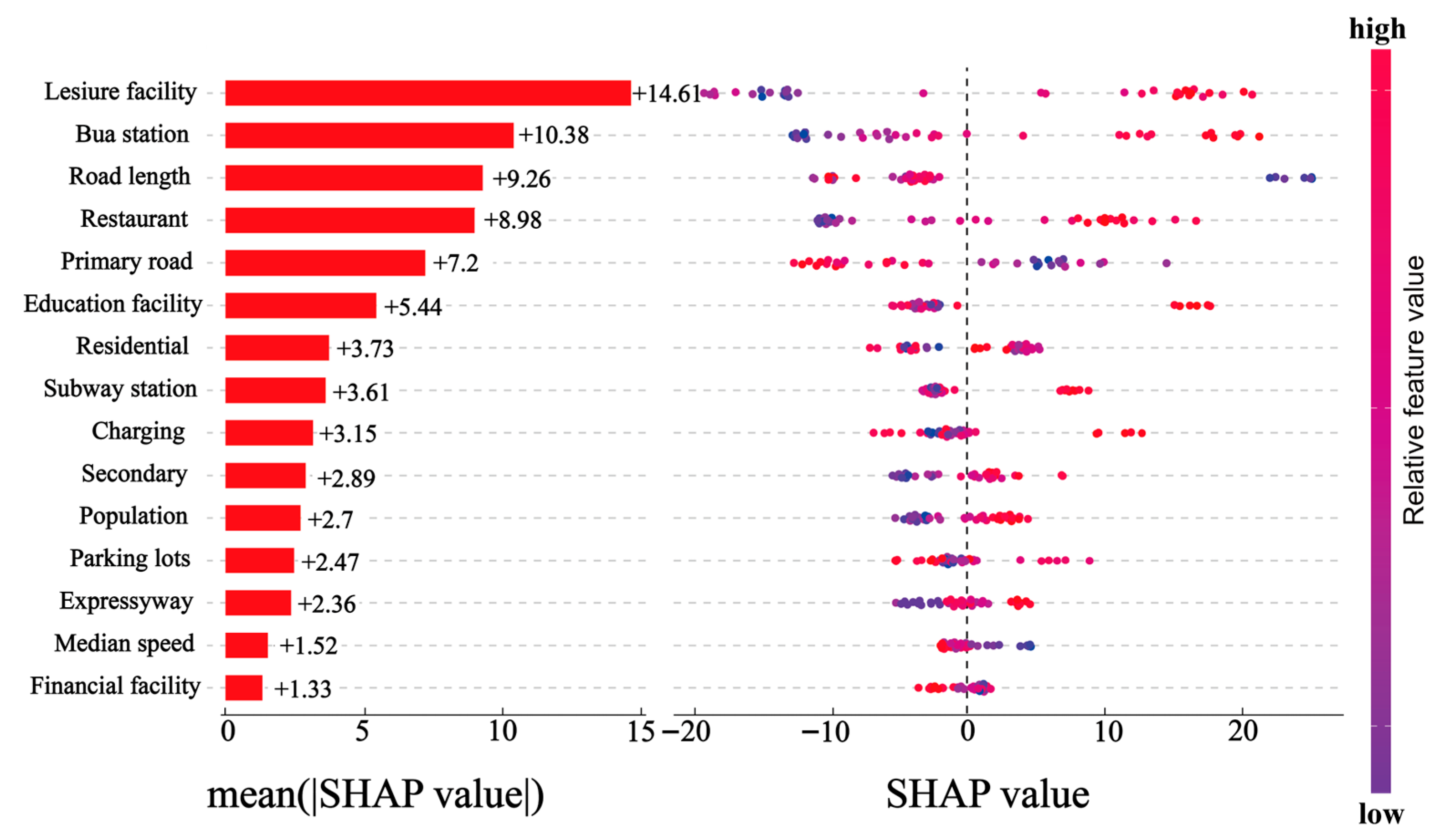
Figure 3 presents the global importance ranking of variables in predicting carbon emissions per unit area across neighborhoods in Ningbo. Among these variables, the density of leisure facilities, bus stations, and road length rank as the top three most influential factors. The subplot on the right side of Figure 3 displays the distribution of feature values for each variable with their corresponding SHAP values. In this plot, the color gradient from red to blue indicates the magnitude of the feature values, while their horizontal position reflects the magnitude of the SHAP values. The figure reveals that land use attributes with higher proportions, specifically leisure facilities, restaurants, and education facilities, tend to have higher SHAP values, suggesting a positive contribution to traffic-related carbon emissions. In contrast, variables such as total road length and the length of primary roads per unit area exhibit a negative effect on carbon emissions.

4.3. Nonlinear Relationships with Built Environment Variables

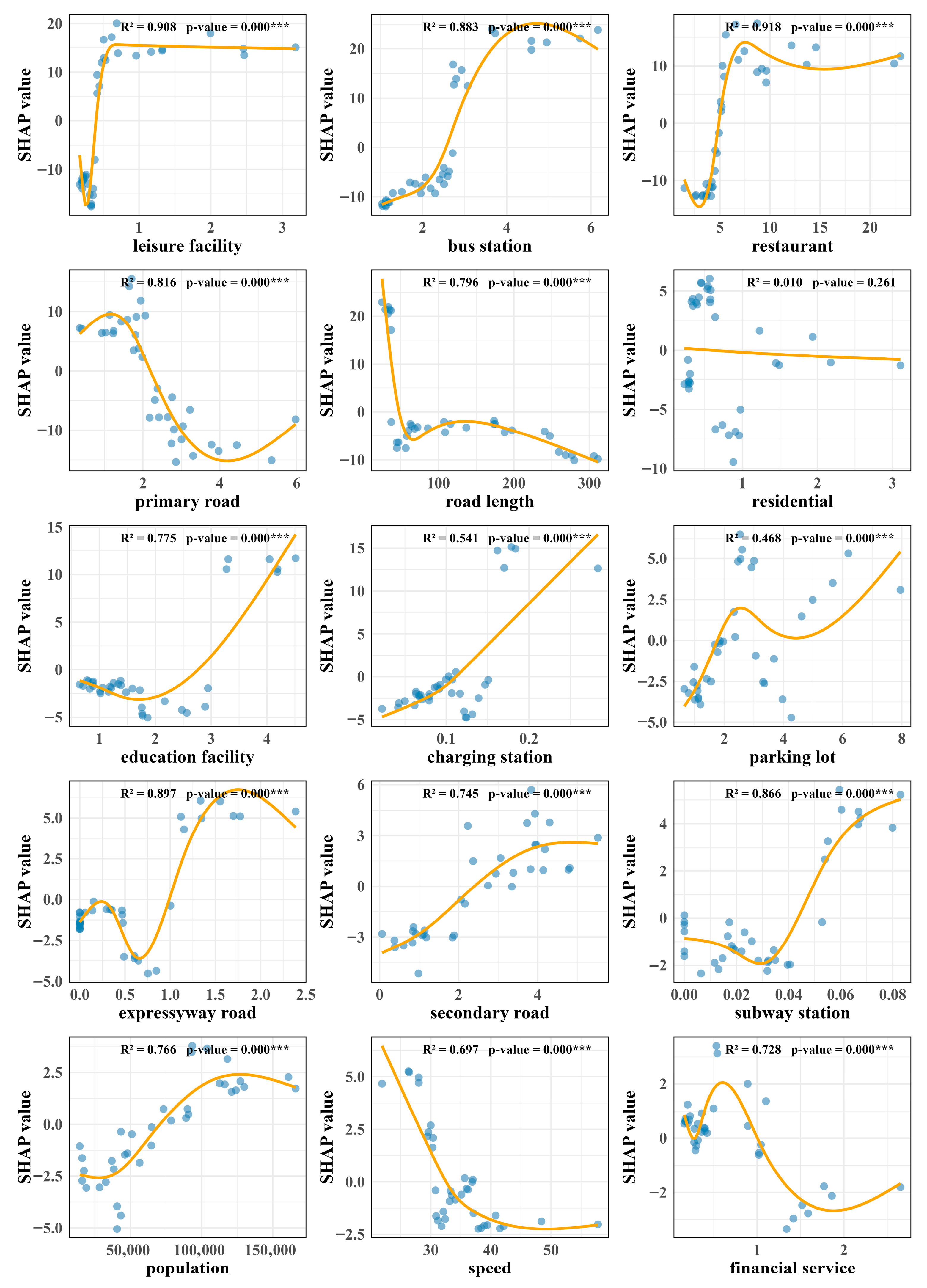
The XGBoost model performs well in capturing the nonlinear relationships between independent and dependent variables. However, it lacks the capacity to interpret these relationships directly. To address this limitation, the SHAP model is employed in this study for interpretability. Figure 4 illustrates the relationships between the feature values and their corresponding SHAP values for 15 selected variables. In addition, this study further applies the GAM to interpret these nonlinear patterns.
The data reveal that, in terms of land use types, both leisure facilities and restaurants exhibit negative SHAP values at low POI densities. However, when their POI densities reach approximately 0.3 POI/km2 and 5 POI/km2, respectively, the SHAP values increase rapidly and then stabilize. This indicates that high POI densities of leisure and dining establishments attract more travel activity, thereby significantly promoting traffic-related carbon emissions. A similar pattern is observed for education facilities, although no clear stabilization of SHAP values is found. In contrast, for neighborhoods with a high POI density of financial services, the SHAP values remain negative, suggesting that a greater concentration of financial service institutions may help suppress traffic emissions to some extent. Regarding road infrastructure, the SHAP values for median vehicle speed are higher when the speed is below approximately 35 km/h. Lower speeds often correspond to more congested traffic conditions, where frequent acceleration, deceleration, and idling contribute to higher carbon dioxide emissions. Both the density of bus stations and subway stations show a similar trend. The low POI density of stations tends to reduce emissions, while a high density of stations is associated with increased emissions. Neighborhoods with high station densities are typically located in city centers and older districts, where high population density and suboptimal road conditions frequently result in congestion during peak hours, thereby increasing traffic emissions. In terms of transportation infrastructure, greater values of total road length and the density of primary road length are associated with a suppression of carbon emission growth, suggesting their potential role in alleviating congestion and improving traffic flow.

4.4. Analysis of Influencing Factors in Specific Urban Functional Areas

Since the selected measurement areas do not fall entirely within a single administrative neighborhood, the SHAP model results are interpreted based on the neighborhoods containing the majority of measurement points. The specific correspondences are as follows: Tianyi Square corresponds to the Jiangxia neighborhood, Laojiangdong corresponds to the Baizhang neighborhood, and the high-tech district corresponds to the Meixu neighborhood.
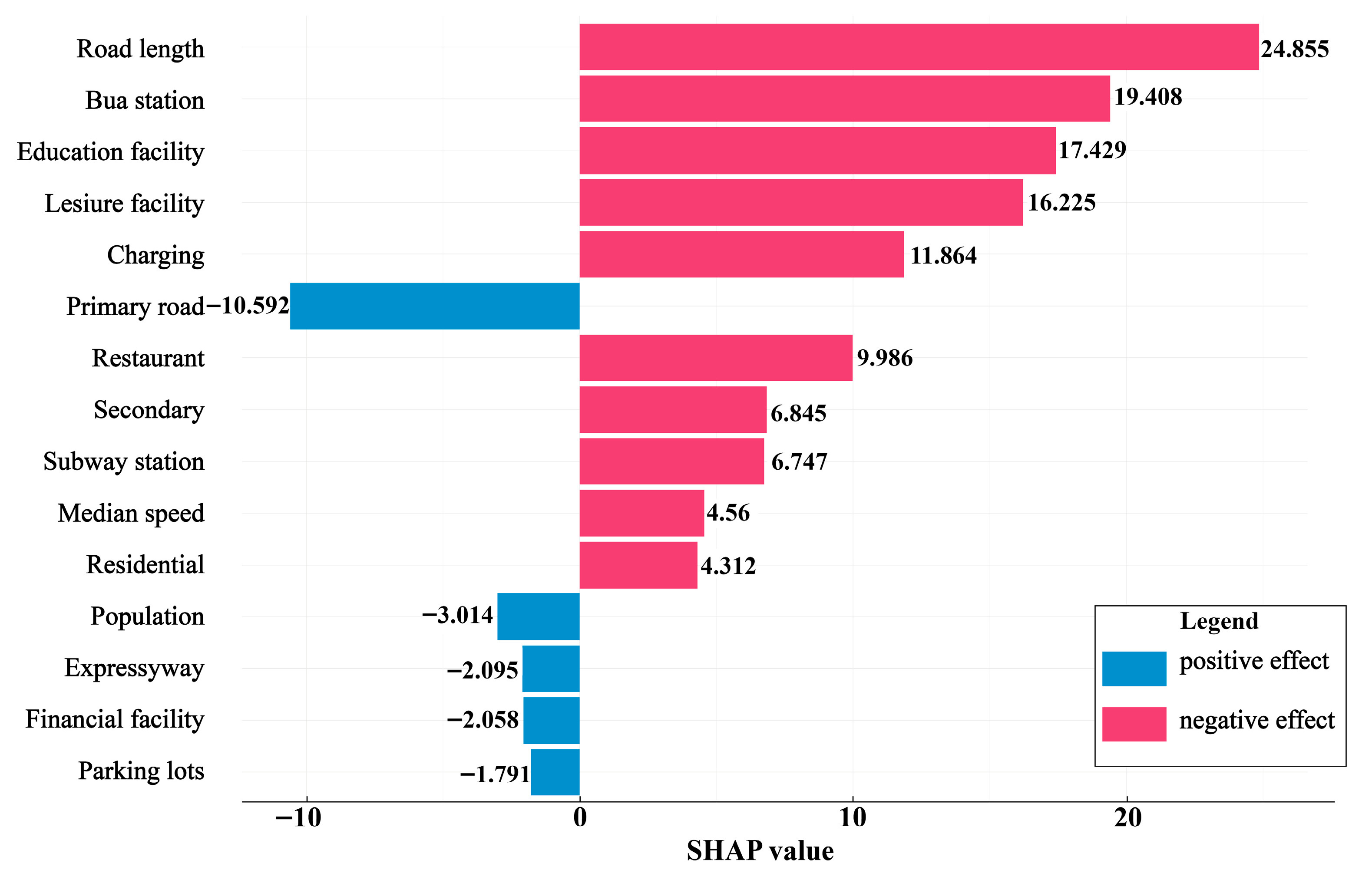
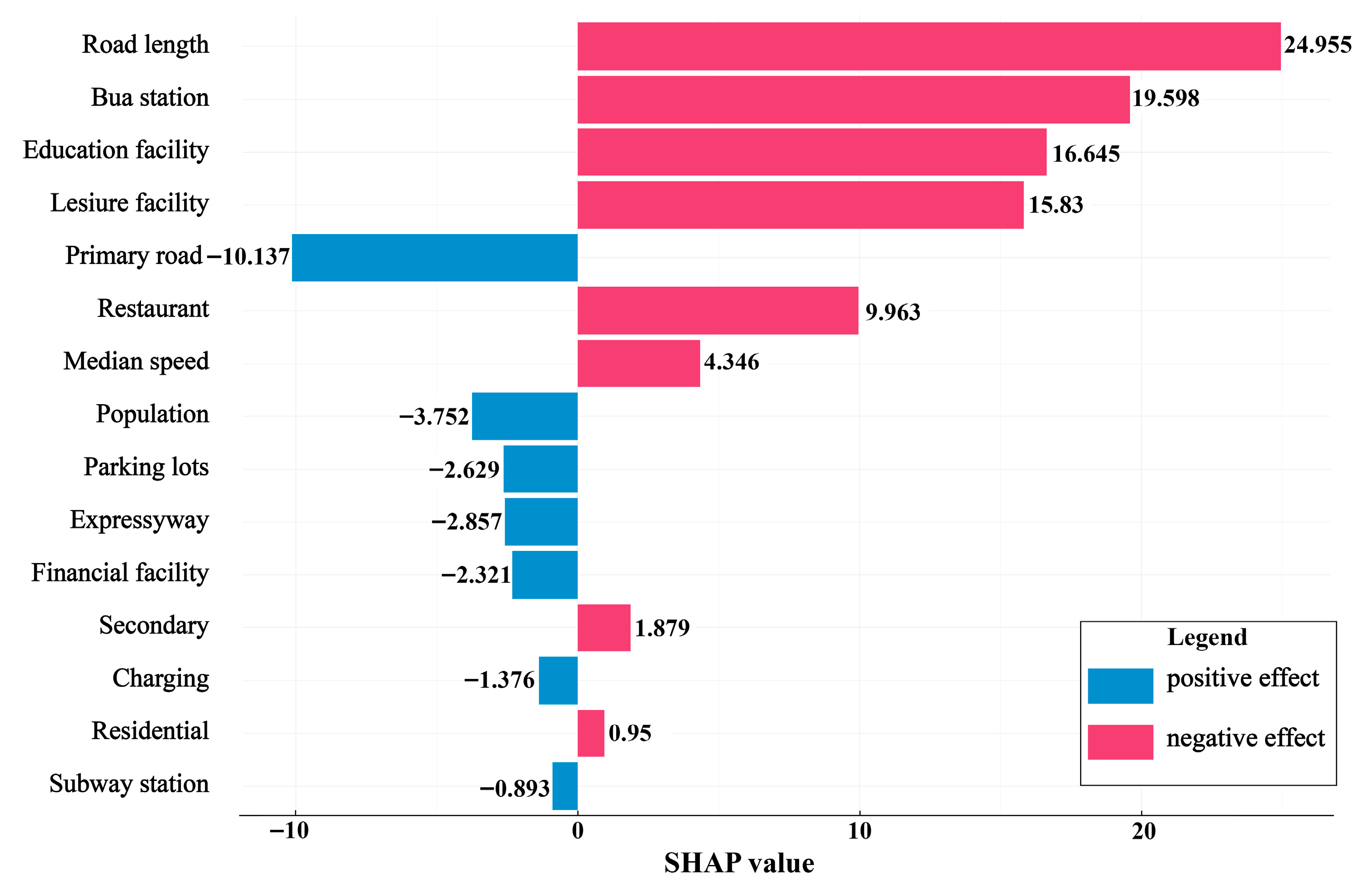
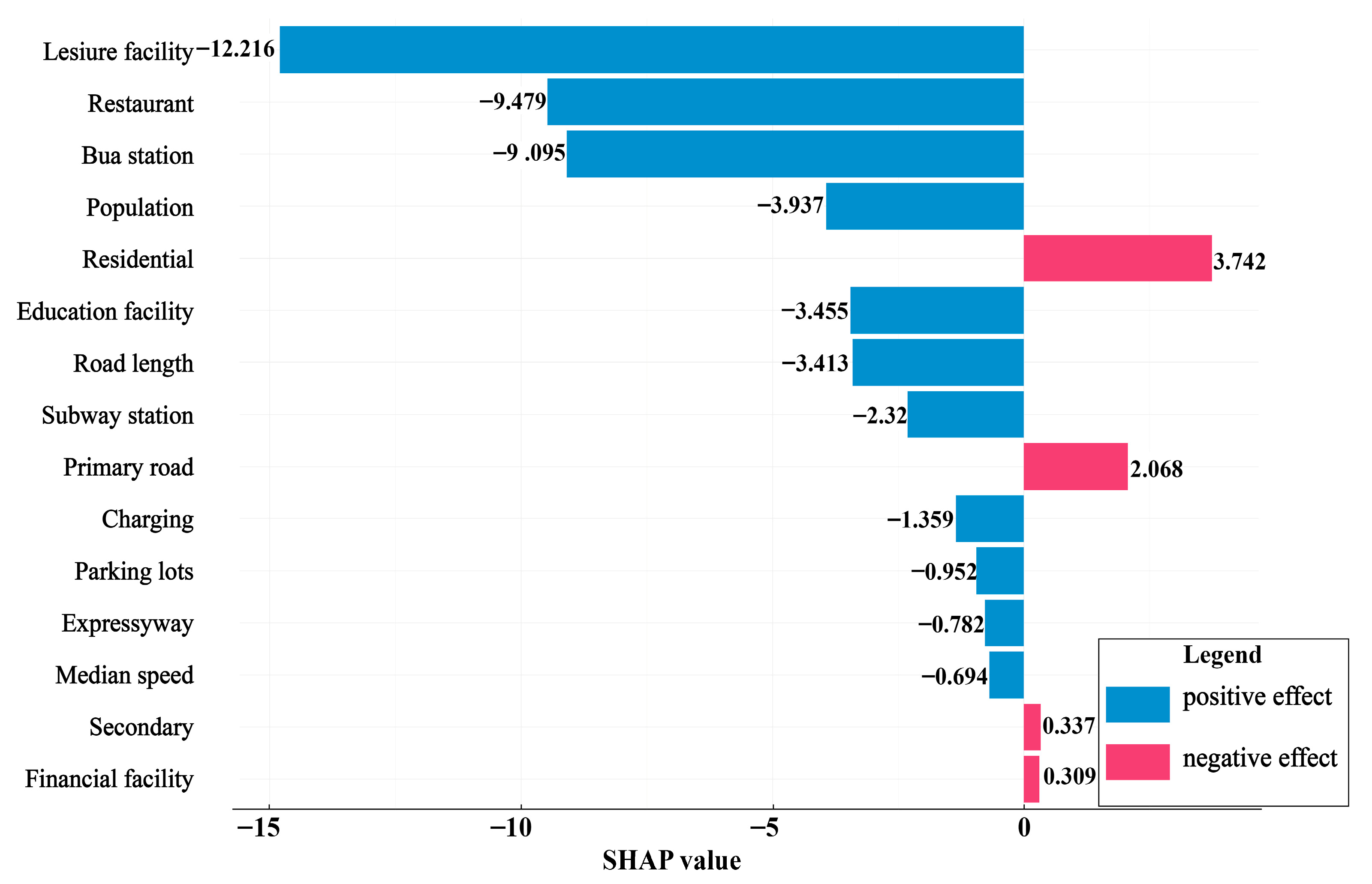
Figure 5 and Figure 6 present the SHAP analysis results for Tianyi Square and Laojiangdong, which, based on land use classification, represent a commercial district and a central urban residential area, respectively. Despite their differing functional roles, the two areas share several common characteristics, including high population density and well-developed transportation infrastructure. A comparative assessment reveals that the SHAP outputs for these two regions are remarkably similar, with the majority of variables exerting a positive influence on traffic-related carbon emissions in both contexts. In such urban environments, leisure facilities and restaurants frequently serve as key attractors of travel demand. In the case of commercial areas, they hold particular appeal for younger populations who predominantly commute by private vehicles and park near commercial complexes—an activity pattern that significantly contributes to elevated traffic emissions. In contrast, Laojiangdong, though situated adjacent to the commercial core, functions primarily as a residential zone. It is characterized by a notably lower density of electric vehicle charging stations, which may lead some residents to seek charging options in other neighborhoods. This spatial deficiency in charging infrastructure appears to exert a suppressive effect on local carbon emissions in older residential areas. Taken together, the findings from these two districts underscore the critical role of the density of primary road length in mitigating traffic-related emissions, reflecting how high-quality road infrastructure can, to some extent, alleviate carbon output from urban traffic. Figure 7 presents the SHAP results for the high-tech zone, an area primarily designated for high-tech industrial development. In this region, leisure facilities and restaurants emerge as the most influential variables. Interestingly, the SHAP patterns observed here are almost the inverse of those in the previous two areas. Due to the relatively homogeneous land use and the scarcity of leisure and dining amenities, the overall potential for increased traffic-induced carbon emissions is significantly reduced. However, the low density of both bus and subway stations in the high-tech zone results in a heavy reliance on private vehicles for commuting. Consequently, the density of primary roads becomes the dominant driver of carbon emission increases in this area.

5. Discussion

Road transport is a major source of urban carbon emissions. Investigating the complex nonlinear effect of the built environment on neighborhood-level road traffic emissions can provide valuable guidance for urban policymakers and planners in designing targeted emission reduction strategies and optimizing spatial planning to achieve sustainable road transport.
Our findings indicate that, at the global level, the relationship between built environment variables and traffic-related carbon emissions exhibits threshold effects, which have also been observed in other Chinese cities [36]. Variables such as population, bus stop density, and subway station density display two thresholds: one in the low-density regime and another in the high-density regime. Across these threshold ranges, both positive and negative effects may occur. In areas with low station density, moderately increasing the number of bus or metro stations can effectively shift travelers from private modes to public transport, thereby reducing traffic-related carbon emissions. However, once density exceeds the upper threshold, over-saturation may lead to operational redundancy and congestion in the vicinity of stations. Related research shows that the densities of bus stops and subway stations account for about 36% of commuting outcomes [37]. In light of the two thresholds identified here, station densities can be adjusted to guide residents toward public transport and thereby reduce emissions.
Across different urban functional zones, the effects of the built environment vary, particularly when comparing residential and commercial areas with high-tech industrial zones. In residential and commercial zones, factors such as the number of bus stops, road length, and the presence of recreational facilities tend to increase traffic-related carbon emissions, whereas they have a mitigating effect in high-tech industrial parks. As the distance from the city center increases, the influence of land use on emissions gradually declines [38], suggesting that more targeted land use adjustments are needed in core areas. Building on the identified thresholds for bus stop and subway station densities, the impacts of the built environment on traffic-related carbon emissions vary markedly across urban functional zones, necessitating differentiated mitigation strategies. In high-density residential and commercial districts, factors such as road-network length and the density of daily service amenities are more sensitive to emissions; priority should therefore be given to compact land use, transit-oriented development (TOD), and parking-demand management. In contrast, in high-tech industrial parks, built environment factors tend to exhibit a mitigating association with emissions, indicating that mitigation in these areas can focus more on improving transport energy efficiency and promoting green logistics systems.
Evidence from Shanghai indicates that optimizing the existing travel modal structure can substantially reduce emissions, but may also generate dissatisfaction with travel costs and service quality [7]. Thus, policymakers should balance emission reductions against user satisfaction. These insights can inform policymakers in Ningbo when allocating land resources and optimizing the public transport structure, thereby helping to maximize the efficient distribution of transit resources and improve service quality.

6. Conclusions and Limitations

This study empirically investigated the nonlinear relationships between carbon emissions and their influencing factors. An interpretable machine learning model was developed to investigate the nonlinear effect of influencing factors by considering the spatially varying effects of the built environment on carbon emissions. Field-measured CO2 concentrations were collected to validate the model results. The findings revealed that the built environment has a dual threshold nonlinear effect on transportation carbon emissions, with one threshold for low-density and one threshold for high-density intervals. The impact effect varies significantly in different land use functional zones, with increased emissions from residential and commercial areas, bus stops, road lengths, and leisure facilities; in high-tech industrial parks, the same variable actually suppresses emissions.
However, this study has certain data-related limitations. Field measurements were collected from only three areas and did not account for weather conditions, which reduces spatial and temporal representativeness. Given that Ningbo is a major port city on China’s eastern coast, the generalizability of the findings to other cities may also be limited. To enhance applicability, future research should collect data over a broader spatial extent and incorporate meteorological variables. It should also extend the analysis of built environment effects on emissions to additional urban functional zones, examine interaction effects among key factors, and further assess robustness using spatial econometric models. As carbon emissions evolve over long time horizons, it is essential to validate and refine the findings in other cities and to deepen the understanding of emission patterns across different functional areas and time periods.

Author Contributions

Methodology: Y.H., C.L. and Y.Z.; software: C.L., Y.F. and J.Z.; validation: C.L.; formal analysis: C.L., Y.F. and J.Z.; investigation: Y.F., J.Z., C.Z., Y.C. and Y.Z.; resources: Y.H.; data curation: Y.F., J.Z. and Y.C.; writing—original draft: C.L., C.Z. and Y.C.; writing—review & editing: Y.H. and C.L.; visualization: C.L. and Y.F.; supervision: Y.H., Y.Z. and S.Z.; project administration: Y.H., Y.Z. and S.Z.; funding acquisition: Y.H. and S.Z. All authors have read and agreed to the published version of the manuscript.

Funding

This study was supported by the Humanities and Social Science Research Project, Ministry of Education, China (23YJCZH085); China-Slovakia Technology Cooperation Committee’s 9th Annual Meeting Personnel Exchange Program of Ministry of Science and Technology of China in the form of an award (9-8); Natural Science Foundation of Zhejiang Province, China (LTGG23E080005); Campus Planning and Construction Project of Zhejiang Province (2023PCBG001); and Research Start-up Foundation of Ningbo University of Technology (2022KQ09). Any opinions, findings, and conclusions or recommendations expressed in this paper are those of the authors and do not necessarily reflect the views of the sponsors.

Data Availability Statement

If necessary, the authors can provide the original data through correspondence.

Conflicts of Interest

The authors declared no potential conflicts of interest with respect to the research, authorship, and/or publication of this article.

Abbreviations

The following abbreviations are used in this manuscript:
MOVESMotor Vehicle Emissions Simulator
XGBoostExtreme Gradient Boosting
SHAPSHapley Additive exPlanations
GAMGeneralized Additive Model
TODTransit-Oriented Development
LightGBM–LIMELight Gradient Boosting Machine–Local Interpretable Model-agnostic Explanations
CatBoost–ALECategorical Boosting–Accumulated Local Effects
RMSERoot Mean Square Error
MAEMean Absolute Error

References

  1. Emissions Gap Report 2024. Available online: https://www.unep.org/resources/emissions-gap-report-2024 (accessed on 3 July 2025).
  2. Li, F.; Cai, B.; Ye, Z.; Wang, Z.; Zhang, W.; Zhou, P.; Chen, J. Changing patterns and determinants of transportation carbon emissions in Chinese cities. Energy 2019, 174, 562–575. [Google Scholar] [CrossRef]
  3. Zhou, W.; Zhou, F.; Zhuang, G. Megacity pathways in China under the dual carbon goal: The case of Shanghai. Chin. J. Popul. Resour. Environ. 2024, 22, 241–249. [Google Scholar] [CrossRef]
  4. Cao, J.; Liu, J.; Cheng, Y.; Ai, S.; Li, F.; Xue, T.; Zhang, Q.; Zhu, T. Impacts of different vehicle emissions on ozone levels in Beijing: Insights into source contributions and formation processes. Environ. Int. 2024, 191, 109002. [Google Scholar] [CrossRef] [PubMed]
  5. Macioszek, E.; Jurdana, I. Bicycle Traffic in the Cities. Sci. J. Silesian Univ. Technol. Ser. Transp. 2022, 117, 115–127. [Google Scholar] [CrossRef]
  6. Sun, S.; Wang, B.; Li, A.R. Shared bicycle study to help reduce carbon emissions in Beijing. Energy Rep. 2020, 6, 837–849. [Google Scholar] [CrossRef]
  7. Zhang, L.; Long, R.; Li, W.; Wei, J. Potential for reducing carbon emissions from urban traffic based on the carbon emission satisfaction: Case study in Shanghai. J. Transp. Geogr. 2020, 85, 102733. [Google Scholar] [CrossRef]
  8. Zhao, H.; Wang, Z.; Luo, J.; Hu, F. Prediction of the effect of bike-sharing on urban carbon emission reduction: Evidence from Beijing. J. Urban Manag. 2025, in press. [Google Scholar] [CrossRef]
  9. Barmpounakis, E.; Montesinos-Ferrer, M.; Gonzales, E.J.; Geroliminis, N. Empirical investigation of the emission-macroscopic fundamental diagram. Transp. Res. Part D Transp. Environ. 2021, 101, 103090. [Google Scholar] [CrossRef]
  10. Rakha, H.A.; Farag, M.; Foroutan, H. Electric versus gasoline vehicle particulate matter and greenhouse gas emissions: Large-scale analysis. Transp. Res. Part D Transp. Environ. 2025, 104, 104622. [Google Scholar] [CrossRef]
  11. Jiang, Y.; Ding, Z.; Zhou, J.; Wu, P.; Chen, B. Estimation of traffic emissions in a polycentric urban city based on a macroscopic approach. Phys. A Stat. Mech. Its Appl. 2022, 602, 127391. [Google Scholar] [CrossRef]
  12. Ji, T.; Li, K.; Sun, Q.; Duan, Z. Urban transport emission prediction analysis through machine learning and deep learning techniques. Transp. Res. Part D Transp. Environ. 2024, 135, 104389. [Google Scholar] [CrossRef]
  13. Liu, B.; Li, F.; Hou, Y.; Antonio Biancardo, S.; Ma, X. Unveiling built environment impacts on traffic CO2 emissions using Geo-CNN weighted regression. Transp. Res. Part D Transp. Environ. 2024, 132, 104266. [Google Scholar] [CrossRef]
  14. Zhang, L.; Lu, G.; Yan, X.; Xia, P.; Chen, Z.; Wu, D. A differential evolution optimized hybrid XGBoost for accurate carbon emission prediction. Environ. Model. Softw. 2025, 193, 106627. [Google Scholar] [CrossRef]
  15. Kwak, K.; Lee, E.H. Impact of road transport system on groundwater quality inferred from explainable artificial intelligence (XAI). Sci. Total Environ. 2024, 917, 170388. [Google Scholar] [CrossRef]
  16. Lee, E.H. Understanding Gender Gap in Bike-Sharing Services via eXplainable Artificial Intelligence. Transp. Res. Rec. J. Transp. Res. Board 2025, 2679, 622–633. [Google Scholar] [CrossRef]
  17. Song, Y.; Zhang, C.; Jin, X.; Zhao, X.; Huang, W.; Sun, X.; Yang, Z.; Wang, S. Spatial prediction of PM2.5 concentration using hyper-parameter optimization XGBoost model in China. Environ. Technol. Innov. 2023, 32, 103272. [Google Scholar] [CrossRef]
  18. Wang, Z.; Wu, X.; Wu, Y. A spatiotemporal XGBoost model for PM2.5 concentration prediction and its application in Shanghai. Heliyon 2023, 9, e22569. [Google Scholar] [CrossRef]
  19. Alfasanah, Z.; Niam, M.Z.H.; Wardiani, S.; Ahsan, M.; Lee, M.H. Monitoring air quality index with EWMA and individual charts using XGBoost and SVR residuals. MethodsX 2025, 14, 103107. [Google Scholar] [CrossRef] [PubMed]
  20. Yang, H.; Xiao, K.; Xiang, X.; Wang, X.; Wang, X.; Du, Y.; Shi, G.; Zheng, X.; Tao, H.; Wang, H.; et al. Prediction of on-road CO2 emissions with high spatio-temporal resolution implementing multilayer perceptron. Atmos. Environ. X 2025, 27, 100368. [Google Scholar] [CrossRef]
  21. Hu, H.; Choi, M.-Y.; Kim, B.; Choi, M.; Kang, S.; Park, H.; Park, M.; Kim, J.; Woo, J.-H. Integrating IAM-based CO2 projections and traffic demand forecasting for regional CO2 emission mapping in the transport sector. Atmos. Pollut. Res. 2025, 102790. [Google Scholar] [CrossRef]
  22. Ouyang, S.; Zhao, P.; Gong, Z. A review of transport carbon emissions: Insights from artificial intelligence and big data. J. Clean. Prod. 2025, 532, 146906. [Google Scholar] [CrossRef]
  23. Khajavi, H.; Rastgoo, A. Predicting the carbon dioxide emission caused by road transport using a Random Forest (RF) model combined by Meta-Heuristic Algorithms. Sustain. Cities Soc. 2023, 93, 104503. [Google Scholar] [CrossRef]
  24. Yang, W.; Qiao, Z.; Wu, L.; Ren, X.; Taghizadeh-Hesary, F. Forecasting carbon dioxide emissions using adjacent accumulation multivariable grey model. Gondwana Res. 2024, 134, 107–122. [Google Scholar] [CrossRef]
  25. Qin, H.; Huang, Q.; Zhang, Z.; Lu, Y.; Li, M.; Xu, L.; Chen, Z. Carbon dioxide emission driving factors analysis and policy implications of Chinese cities: Combining geographically weighted regression with two-step cluster. Sci. Total Environ. 2019, 684, 413–424. [Google Scholar] [CrossRef]
  26. Wu, J.; Jia, P.; Feng, T.; Li, H.; Kuang, H.; Zhang, J. Uncovering the spatiotemporal impacts of built environment on traffic carbon emissions using multi-source big data. Land Use Policy 2023, 129, 106621. [Google Scholar] [CrossRef]
  27. Peng, Z.; Zhao, J.; Ji, H.; Wang, Y.; Wang, C.; Easa, S. Evaluating spatial effect of transportation planning factors on taxi CO2 emissions. Sci. Total Environ. 2025, 959, 178142. [Google Scholar] [CrossRef]
  28. Zhi, D.; Zhao, H.; Chen, Y.; Song, W.; Song, D.; Yang, Y. Quantifying the heterogeneous impacts of the urban built environment on traffic carbon emissions: New insights from machine learning techniques. Urban Clim. 2024, 53, 101765. [Google Scholar] [CrossRef]
  29. Yang, W. The nonlinear effects of multi-scale built environments on CO2 emissions from commuting. Transp. Res. Part D Transp. Environ. 2023, 118, 103736. [Google Scholar] [CrossRef]
  30. Yun, H.; Lee, E.H. Party politics in transport policy with a large language model. Transp. Policy 2025, 171, 487–496. [Google Scholar] [CrossRef]
  31. Lee, E.H. eXplainable DEA approach for evaluating performance of public transport origin-destination pairs. Res. Transp. Econ. 2024, 108, 101491. [Google Scholar] [CrossRef]
  32. Ningbo Data Open Platform. Available online: http://data.ningbo.gov.cn/nbdata/fore/index.html/#/home?t=1678288126718&id=1 (accessed on 29 November 2024).
  33. OpenStreetMap. Available online: https://vdatahub.mapplus.cn/export#map=6/26.224/110.874 (accessed on 29 November 2024).
  34. Amap. Available online: https://lbs.amap.com/ (accessed on 3 December 2024).
  35. Emissions Database for Global Atmospheric Research. European Commission, Joint Research Centre (JRC). Available online: https://data.jrc.ec.europa.eu/dataset/c0c49cd7-4a80-4a94-8c34-375289c12b2d (accessed on 11 July 2024).
  36. Wu, J.; Jia, P.; Feng, T.; Li, H.; Kuang, H. Spatiotemporal analysis of built environment restrained traffic carbon emissions and policy implications. Transp. Res. Part D Transp. Environ. 2023, 121, 103839. [Google Scholar] [CrossRef]
  37. Ding, C.; Liu, T.; Cao, X.; Tian, L. Illustrating nonlinear effects of built environment attributes on housing renters’ transit commuting. Transp. Res. Part D Transp. Environ. 2022, 112, 103503. [Google Scholar] [CrossRef]
  38. Zhang, Y.; Zhou, W. Nonlinear and interactive effects of complex built environment on travel-related CO2 emissions. Sustain. Cities Soc. 2025, 130, 106574. [Google Scholar] [CrossRef]
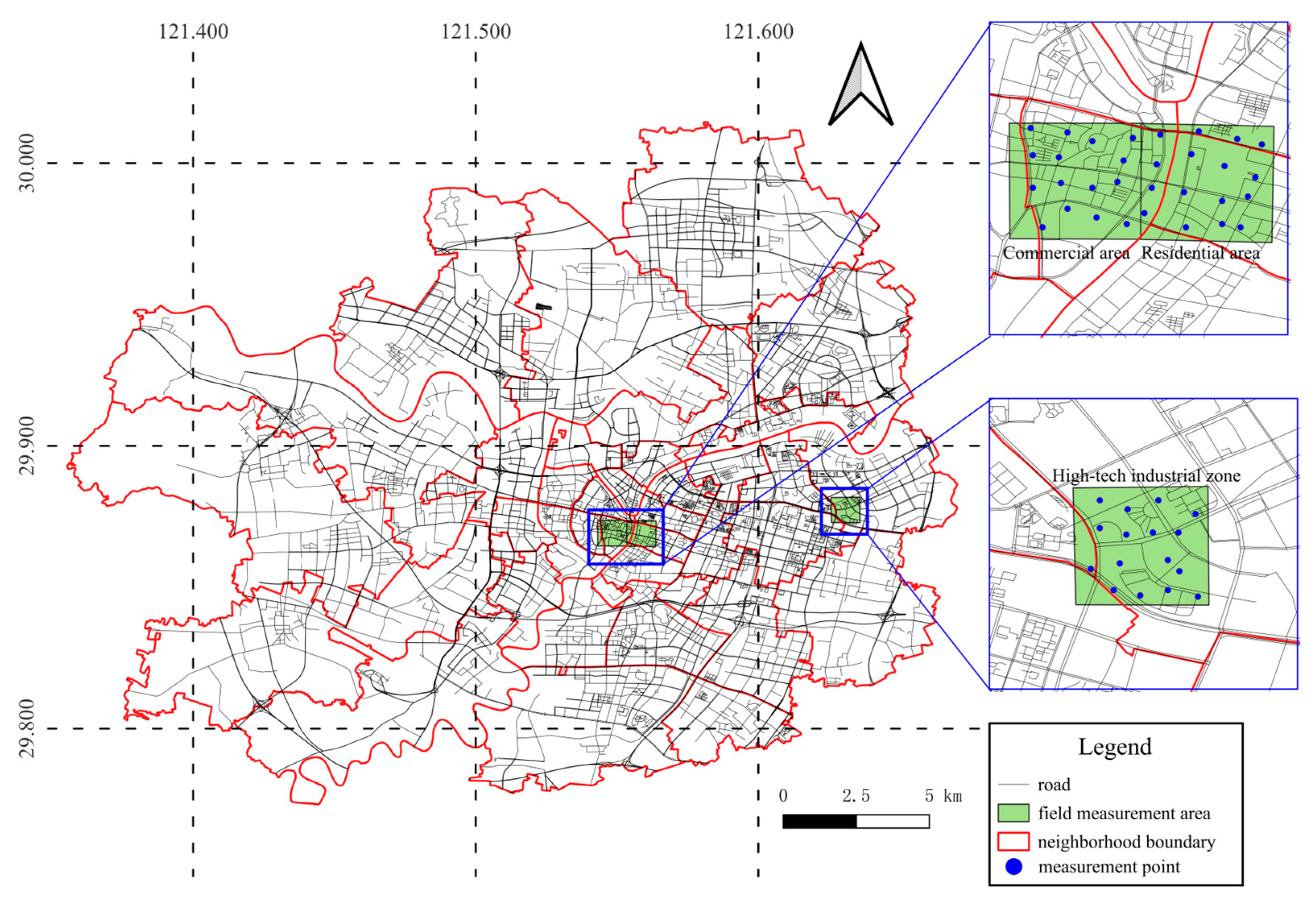
Figure 1. Study area and road network map. Note: Base map and spatial data are downloaded from OpenStreetMap and Amap.
Sustainability 17 10819 g001
Figure 2. Research framework. Note: *** represents significance at 0.001.
Sustainability 17 10819 g002
Figure 3. Results of SHAP analysis by carbon emission per unit area.
Sustainability 17 10819 g003
Figure 4. SHAP dependence analysis on carbon emission. Note: *** represents significance at 0.001. The blue dots represent the eigenvalues of the variables. The orange line represents the GAM fitting result.
Sustainability 17 10819 g004
Figure 5. Results of SHAP model for commercial area.
Sustainability 17 10819 g005
Figure 6. Results of SHAP model for residential area.
Sustainability 17 10819 g006
Figure 7. Results of SHAP model for high-tech industrial zone.
Sustainability 17 10819 g007
Table 1. Variables description.
Variable Description Source
PopulationPopulation per neighborhoodNingbo Data Open Platform [32]
Road lengthRoad length in neighborhoods (km)Open Street Map [33]
Expressway road densityLength of expressway road per unit area (km/km2)Open Street Map
Primary road densityLength of primary road per unit area (km/km2)Open Street Map
Secondary road densityLength of secondary road per unit area (km/km2)Open Street Map
Parking lot densityThe number of parking lots per unit road length (POI/km)Amap POI [34]
Bus station densityThe number of bus stations per unit road length (POI/km)Amap POI
Subway station densityThe number of subway stations per unit road length (POI/km)Amap POI
Residential area densityThe number of residential areas per unit road length (POI/km)Amap POI
Charging station densityThe number of charging stations per unit road length (POI/km)Amap POI
Restaurant densityThe number of restaurants per unit road length (POI/km)Amap POI
Leisure facility densityThe number of leisure facilities per unit road length (POI/km)Amap POI
Financial service densityThe number of financial services per unit road length (POI/km)Amap POI
Education facility densityThe number of education facilities per unit road length (POI/km)Amap POI
Median speed Median vehicle speed (km/h)Ningbo Data Open Platform
Table 2. CO2 concentrations from three selected areas.
Measure AreaBackground Concentration of CO2 (ppm)Concentration of Traffic CO2 Beside Road (ppm)
Tianyi Square district435.21470.44
High-tech district425.68446.40
Laojiangdong district426.20449.24
Table 3. Results of prediction.
Measure AreaFunction AreaConcentration of Traffic CO2 (ppm)Prediction of Carbon Emissions (t/km2)
Tianyi SquareCommercial area24.22164
High-tech districtHigh-tech industrial zone20.72101.06
Laojiangdong districtResidential area23.04161.75
Disclaimer/Publisher’s Note: The statements, opinions and data contained in all publications are solely those of the individual author(s) and contributor(s) and not of MDPI and/or the editor(s). MDPI and/or the editor(s) disclaim responsibility for any injury to people or property resulting from any ideas, methods, instructions or products referred to in the content.