A Green Vehicle Routing Problem with Time-Varying Speeds and Joint Distribution

Abstract

With the rapid growth of urban logistics demand, carbon emissions and the time-varying nature of vehicle speeds have become critical challenges in sustainable transportation planning. This paper addresses a Time-Dependent Green Vehicle Routing Problem (TDGVRP) that integrates time-varying speeds, carbon emissions, and cold chain logistics under a joint distribution framework involving multiple depots and homogeneous refrigerated vehicles. A Mixed-Integer Linear Programming (MILP) model is developed, explicitly considering carbon pricing, refrigeration energy consumption, and speed variations across different time periods. To efficiently solve large-scale instances, a Three-Phase Heuristic (TPH) algorithm is proposed, combining spatiotemporal path construction, local-improvement strategies, and an Adaptive Large Neighborhood Search (ALNS) mechanism. Computational experiments show that the proposed method outperforms traditional Genetic Algorithms (GAs) in both solution quality and computation time, and in some benchmark cases even achieves better results than the commercial solver Gurobi, demonstrating its robustness and scalability. Using real-world traffic speed data, comparative analysis reveals that the joint distribution strategy reduces total logistics costs by 14.40%, carbon emission costs by 23.12%, and fleet size by approximately 25% compared to single-entity distribution. The findings provide a practical and scalable solution framework for sustainable cold chain logistics routing in time-dependent urban road networks.

1. Introduction

The transportation sector’s heavy reliance on fossil fuels has made it one of the fastest-growing sources of Global Greenhouse Gas (GHG) emissions. Reducing GHG emissions, particularly carbon dioxide (CO₂), has become an urgent and common objective in mitigating the impacts of climate change [1,2]. According to the Intergovernmental Panel on Climate Change 2022 report, the transportation sector accounted for 15% of global anthropogenic GHG emissions and 23% of energy-related emissions in 2019. The sector produced approximately 870 million tonnes of CO₂ equivalent in that year, and this is projected to grow to between 16% and 50% by 2050.

Compared to conventional transportation, cold chain logistics exacerbates emission challenges due to its continuous refrigeration demands for maintaining low temperatures to preserve product quality. Adakemaya et al. [3] estimate that approximately 40% of transported food requires refrigeration, accounting for 53% of total energy consumption in transportation. According to Allied Market Research (2019) [3], the global cold chain logistics market reached USD 160 billion in 2018 and is expected to exceed USD 585 billion by 2026, with a Compound Annual Growth Rate (CAGR) of 17.9%. Against the backdrop of China’s dual carbon strategy, green transformation has become an imperative, and carbon reduction in cold chain logistics is both a challenge and an opportunity for sustainable development.

Despite rapid growth, the cold chain logistics sector in China remains fragmented, with low integration across firms. This inefficiency results in poor network coordination, excessive resource consumption, and significant avoidable carbon emissions, reportedly costing tens of billions of yuan annually [4]. Traditional “supply-driven” operational models are increasingly unsustainable. In this context, joint distribution—a model in which multiple logistics enterprises share transportation resources and customer bases under unified planning and scheduling [5]—has emerged as a promising approach. From an industry perspective, joint distribution can significantly reduce total logistics costs and carbon emissions through optimized resource allocation [6]. However, most VRP studies adopt a single-enterprise perspective, neglecting the systemic benefits of collaborative resource sharing in cold chain logistics. This omission has left a gap in quantifying industry-wide cost and emission reductions achievable through joint distribution.

Route planning serves as a vital lever for improving transportation system efficiency. Studies have shown that optimizing vehicle flow distribution and alleviating congestion can significantly reduce fuel consumption, emissions, and time-related costs without requiring additional infrastructure investment [7]. For cold chain logistics, where delivery delays can directly cause product spoilage, route optimization must not only minimize travel time but also incorporate energy efficiency, carbon control, and industry-level collaboration.

The Vehicle Routing Problem (VRP), initially developed to optimize delivery schedules and minimize transportation costs [8], has evolved to include multiple variations such as time windows, multiple depots, and heterogeneous fleets. In cold chain contexts, additional constraints such as spoilage rate, refrigeration cost, and carbon emissions have been incorporated into routing models [9,10], while some studies introduce carbon trading and taxation mechanisms into the optimization framework [11,12,13]. Nonetheless, research gaps remain: (1) Most models consider only a single enterprise, overlooking the collaborative potential of joint distribution in cold chain logistics. (2) Many models assume static traffic conditions and fail to account for time-dependent urban congestion. (3) Scale flexibility is rarely addressed, limiting adaptability to dynamic operational demands. (4) Single-objective optimization dominates, whereas practical cold chain operations require multi-objective trade-offs among cost, time, and emissions.

To address these gaps, this paper proposes a Time-Dependent Green Vehicle Routing Problem (TDGVRP) that incorporates joint distribution and time-dependent traffic conditions into a multi-objective optimization framework. The key contributions of this study are as follows:

• Developing a cross-enterprise joint distribution framework based on depot location and customer clustering.
• Proposing a piecewise time-dependent travel time function to reflect real-world urban traffic dynamics.
• Designing a three-phase heuristic algorithm composed of space–time clustering for zone partitioning, a greedy method for initial route allocation, and an Adaptive Large Neighborhood Search (ALNS) for route refinement and repair.
• Conducting a joint cost analysis that captures the time-sensitive relationship between energy consumption and carbon emissions under various routing decisions.

Overall, this research aims to enhance cold chain logistics efficiency and promote its low-carbon transformation by integrating joint distribution mechanisms with time-dependent routing optimization.

The remainder of this paper is organized as follows: Section 2 presents a comprehensive literature review. Section 3 introduces the research objectives and develops the mathematical model. Section 4 describes the proposed three-phase heuristic algorithm in detail. Section 5 conducts the experimental design and analyzes the results. Finally, Section 6 summarizes the main findings and outlines potential directions for future research.

2. Literature Review

The VRP remains a cornerstone of logistics optimization, with recent research extending beyond cost/distance minimization to incorporate environmental sustainability, joint distribution, and multi-objective trade-offs. This section reviews (1) time-dependent VRP, (2) low-carbon VRP, (3) multi-objective VRP, and (4) green collaborative cold-chain routing.

2.1. Time-Dependent Vehicle Routing Problem

Traditional VRP models often assume fixed travel speeds, which is insufficient for capturing real-world traffic dynamics. The TDVRP incorporates time-varying travel speeds by associating velocity with departure time through time-dependent speed functions, offering a more realistic representation of traffic conditions.

Pan et al. [14] formulated a Multi-Trip TDVRP with Time Windows (MT-TDVRPTW) and developed a hybrid metaheuristic algorithm. Gmira et al. [15] addressed the TDVRP with time windows by considering time-dependent shortest paths and applied a tabu search-based heuristic to solve the problem. In addition, Zhao et al. [16] and Ma et al. [17] introduced deep learning approaches (e.g., GRU, CNN-LSTM) to forecast short-term urban traffic speeds, providing real-time inputs for dynamic routing decisions.

2.2. Low-Carbon Vehicle Routing Problem

In response to growing environmental concerns, carbon emissions have been incorporated into VRP models, giving rise to the LCVRP. The objective is to minimize greenhouse gas emissions while maintaining logistical efficiency.

Alinaghian et al. [18] proposed an integrated framework combining enhanced tabu search and differential evolution to address a low-carbon inventory-routing problem.

Ferreira et al. [19] developed a heuristic and branch-and-cut method for LCVRP with split deliveries. Li et al. [20] studied the impact of carbon taxes and emission quotas on bi-objective VRP and proposed a hybrid genetic-tabu search algorithm. Liu et al. [21] addressed vehicle routing with heterogeneous fuel types, while Pu et al. [22] formulated a multi-objective LCVRP for intra-city distribution considering fuel cost, emission cost, and distance, solved by an improved chemical reaction optimization algorithm.

2.3. Multi-Objective Vehicle Routing Problem

Multi-objective optimization has gained traction as real-world applications often require balancing conflicting goals such as cost, service level, and environmental impact.

Ghannadpour and Zarrabi [23] constructed a bi-objective model focusing on fuel consumption and customer service priority, aiming to minimize total distance, fleet size, and fuel usage while maximizing customer satisfaction. Sun et al. [24] proposed an optimization algorithm based on Economical Traveling Distance to optimize the configuration of a heterogeneous vehicle fleet for minimizing fuel costs. Zarouk et al. [25] developed a model under soft time windows to minimize energy consumption and maximize satisfaction using a hybrid genetic-simulated annealing algorithm. These works underscore the importance of multi-objective frameworks for sustainable logistics.

2.4. Green and Collaborative Routing in Cold Chain Logistics

Cold chain logistics demands temperature-controlled transport, leading to high energy consumption and costs—over 40% of food requires refrigeration, which accounts for more than half of operational expenses [3]. Consequently, GVRPs have been developed to integrate environmental factors, such as CO₂ emissions [11,12,13,18,26,27,28].

However, most cold chain operations still use independent distribution, resulting in low vehicle utilization and high costs [9,29]. Joint distribution—where multiple companies share resources under centralized coordination—has shown promise in improving efficiency, reducing transport distance, cost, and emissions [6,27,30,31,32,33].

Despite these advances, few studies integrate joint distribution with time-dependent traffic conditions, often treating them separately. Bridging this gap is key to achieving efficient, scalable, and low-carbon cold chain logistics. This study addresses these gaps by (1) modeling time-dependent speeds across periods, (2) integrating joint distribution strategies to improve load rates and reduce emissions, and (3) proposing a three-phase heuristic tailored for large-scale, real-time cold chain routing problems. This approach supports green, efficient, and scalable logistics systems.

3. Problem Statement

3.1. Problem Description

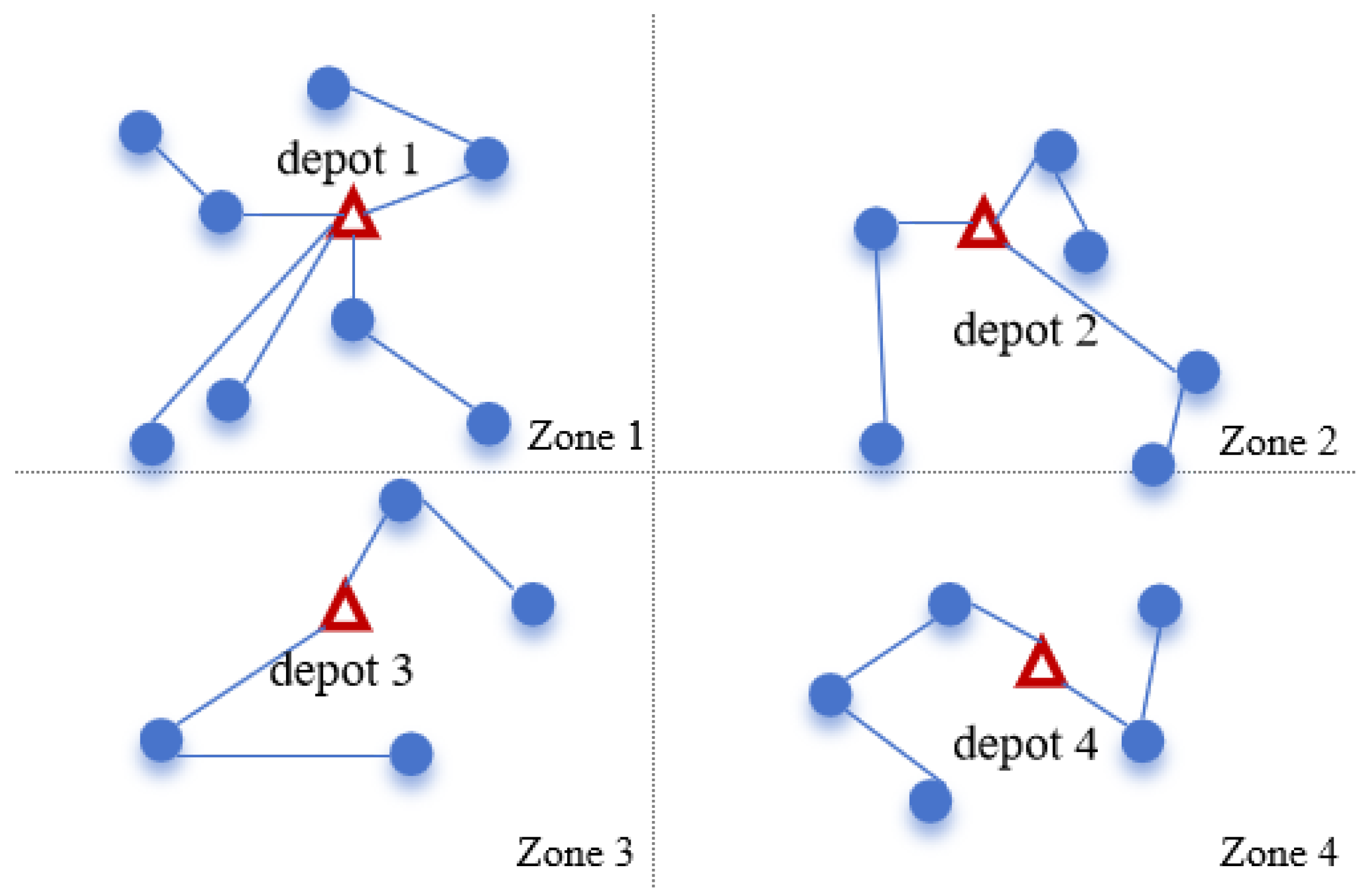
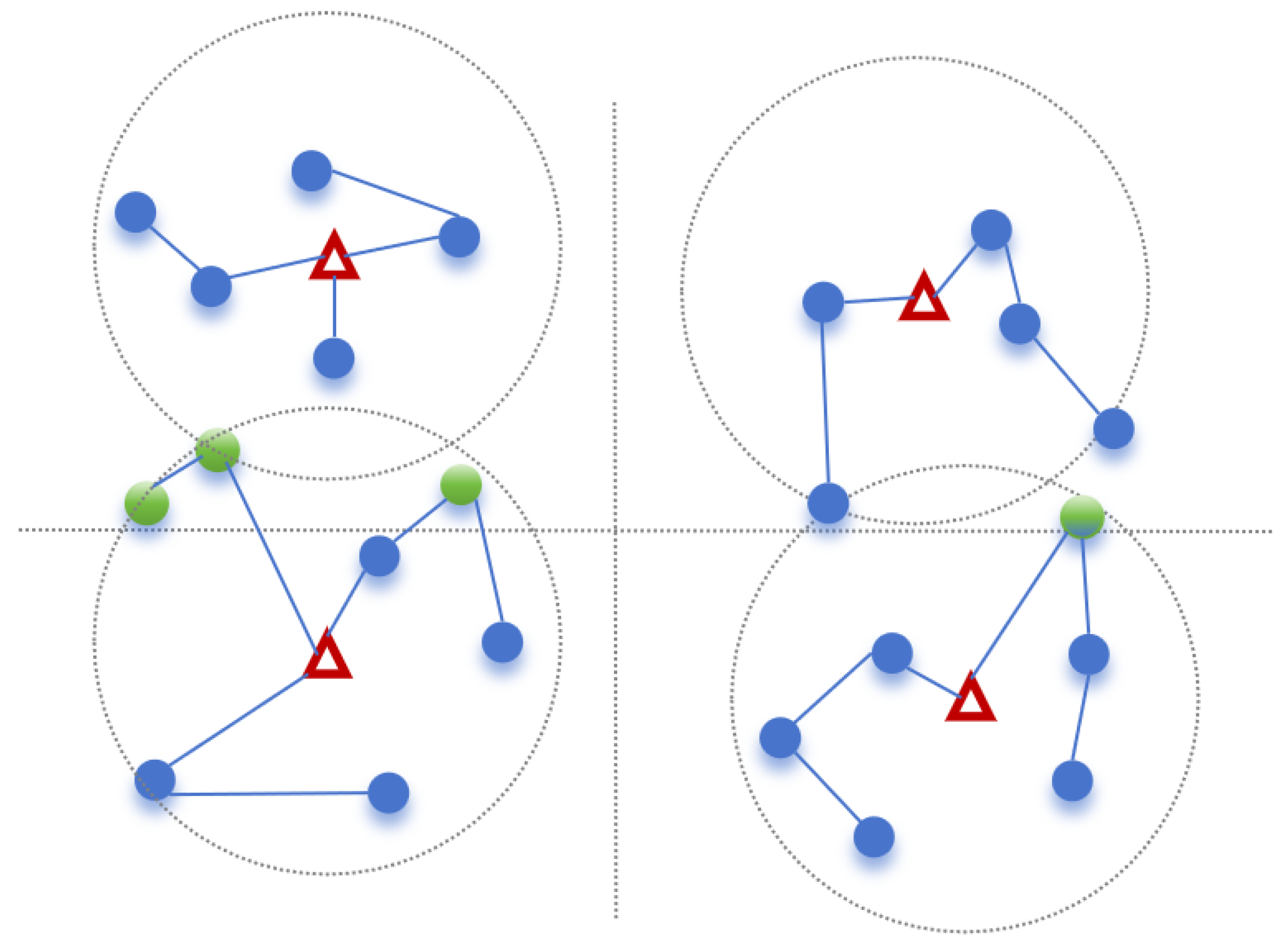
In practical operations, multiple cold-chain logistics companies typically operate their own warehouses and serve customers within designated regions, as illustrated in Figure 1 and Figure 2. Generally, there are two distribution modes: independent distribution, where each company uses its own fleet to serve its customers without any collaboration between companies; and collaborative distribution, where all companies share warehouses, fleets, and customer resources. This paper focuses on the collaborative distribution model.

The formulation of the Time-Dependent Green Vehicle Routing Problem (TDGVRP) is based on the following assumptions:

(1)

The geographic location, product demand, and preferred delivery time window of each customer are known.

(2)

There are multiple distribution centers, and all vehicles are homogeneous refrigerated trucks.

(3)

Vehicles may depart from a distribution center at any time as needed.

(4)

Distribution centers have sufficient inventory and transportation capacity to fulfill delivery tasks.

(5)

Overloading is not allowed during delivery, and customer demand cannot be split.

(6)

The urban road network is time-dependent; that is, vehicles travel at different speeds in different traffic periods depending on the level of congestion.

(7)

All delivery vehicles start from a distribution center and return to the same center after completing their delivery tasks.

(8)

Vehicles have a fixed usage cost, and during distribution incur travel time costs, waiting time costs, and service time costs based on their total usage time (including travel, waiting, and service).

3.2. Travel Speed and Time-Dependent Travel Time Calculation

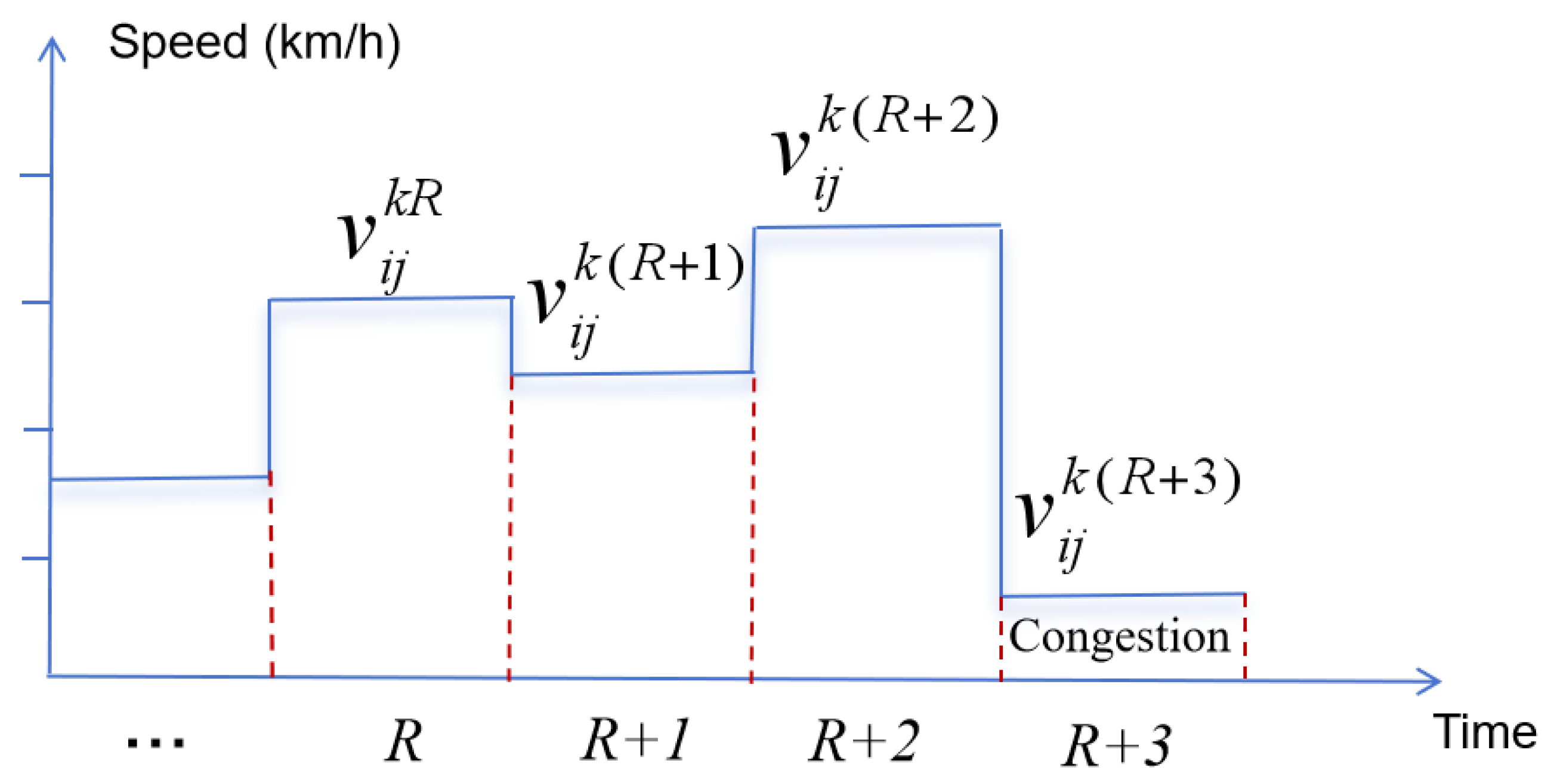
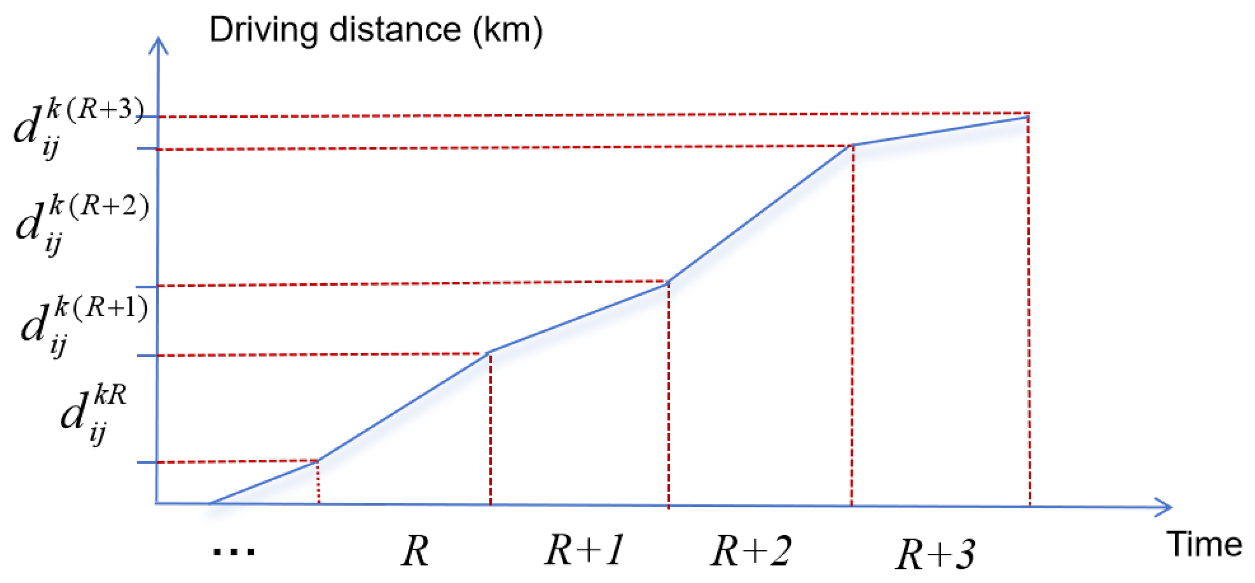
The traffic conditions of an urban road network are influenced by time. For example, during morning and evening peak hours, roads become heavily congested and vehicle speeds slow down, while in other periods speeds are also affected to some extent by traffic flow. Therefore, the travel speed of delivery vehicles is time-dependent. In addition, a delivery vehicle may need to cross multiple time periods to complete travel on a given road segment, making it difficult to directly calculate the travel time for that segment and requiring an appropriate handling method. Methods for calculating vehicle travel time are mainly based on the Malandraki model [34] and the Ichoua model [35]. Since the traffic conditions in our study satisfy the First In, First Out (FIFO) property, the Ichoua model is applicable. Moreover, several studies, such as Jabali [36], Xiao and Konak [37], and Franceschetti et al. [38], have adopted this model to investigate vehicle travel times under time-dependent road network conditions. Accordingly, this study adopts the Ichoua-based approach to analyze the relationships between time periods, time-dependent vehicle speeds, road segment lengths, travel distances, and travel times. First, the operating hours of the distribution center are evenly divided into multiple time periods. Then, following the FIFO principle, a method is designed to calculate travel times for road segments that span multiple periods (as illustrated in Figure 3 and Figure 4): Figure 3 shows the travel speed of delivery vehicles on segment $(i,j)$ during different time periods. Figure 4 shows the travel distance and travel time of delivery vehicles on segment $(i,j)$ during different time periods. Based on the vehicle speeds in each period from Figure 3 and the travel distances in each period from Figure 4, the travel time for each period can be computed, thereby determining the total travel time required for a vehicle to traverse segment $(i,j)$.

To compute the time-dependent travel time of segment $(i,j)$, the operating time horizon T of the distribution center is divided into H discrete periods of equal length $\gamma$, forming discrete time slots $T=\{t_0,t_0+\gamma ,\dots ,t_0+H\gamma \}$, where each time slot is indexed as $T_h$ with $h\in \{1,2,\dots ,H\}$. Each slot represents a time interval $[t_h,t_{h+1}]$.

When a vehicle travels along arc $(i,j)$, it may cross one or multiple consecutive time slots. Let $v_{ij}^h$ represent the travel speed on arc $(i,j)$ during time slot $T_h$, and let $s_j$ denote the service time at node j. The time-dependent travel time function ${\tau }_{ij}\left({\mathrm{dep}}_i\left(t\right)\right)$ is defined as:

$${\tau }_{ij}\left({\mathrm{dep}}_j\left(t\right)\right)=\left\{\begin{array}{cc}{L}_{ij}/v_{ij}^{h_a}+s_j,\hfill & \mathrm{if}{h}_a=h_b\hfill \\ {\mathrm{arr}}_j\left(t\right)-{\mathrm{arr}}_i\left(t\right)+s_j,\hfill & \mathrm{if}{h}_b=h_a+1\hfill \\ (T_{h_{a+1}}-{\mathrm{arr}}_i\left(t\right))+(h_b-h_a-1)\gamma +({\mathrm{arr}}_j\left(t\right)-T_{h_b})+s_j,\hfill & \mathrm{if}{h}_b>h_a+1\hfill \end{array}\right.$$

(1)

Here, ${\mathrm{arr}}_i\left(t\right)$ represents the departure time from node i. The detailed interpretation of ${\tau }_{ij}(·)$ is as follows:

• When $h_a=h_b$, the travel occurs entirely within a single time slot. The travel time between nodes i and j is simply the arc length divided by the speed in that time slot:

  $${\tau }_{ij}={\displaystyle \frac{L_{ij}}{v_{ij}^{h_a}}}+s_j$$

  (2)
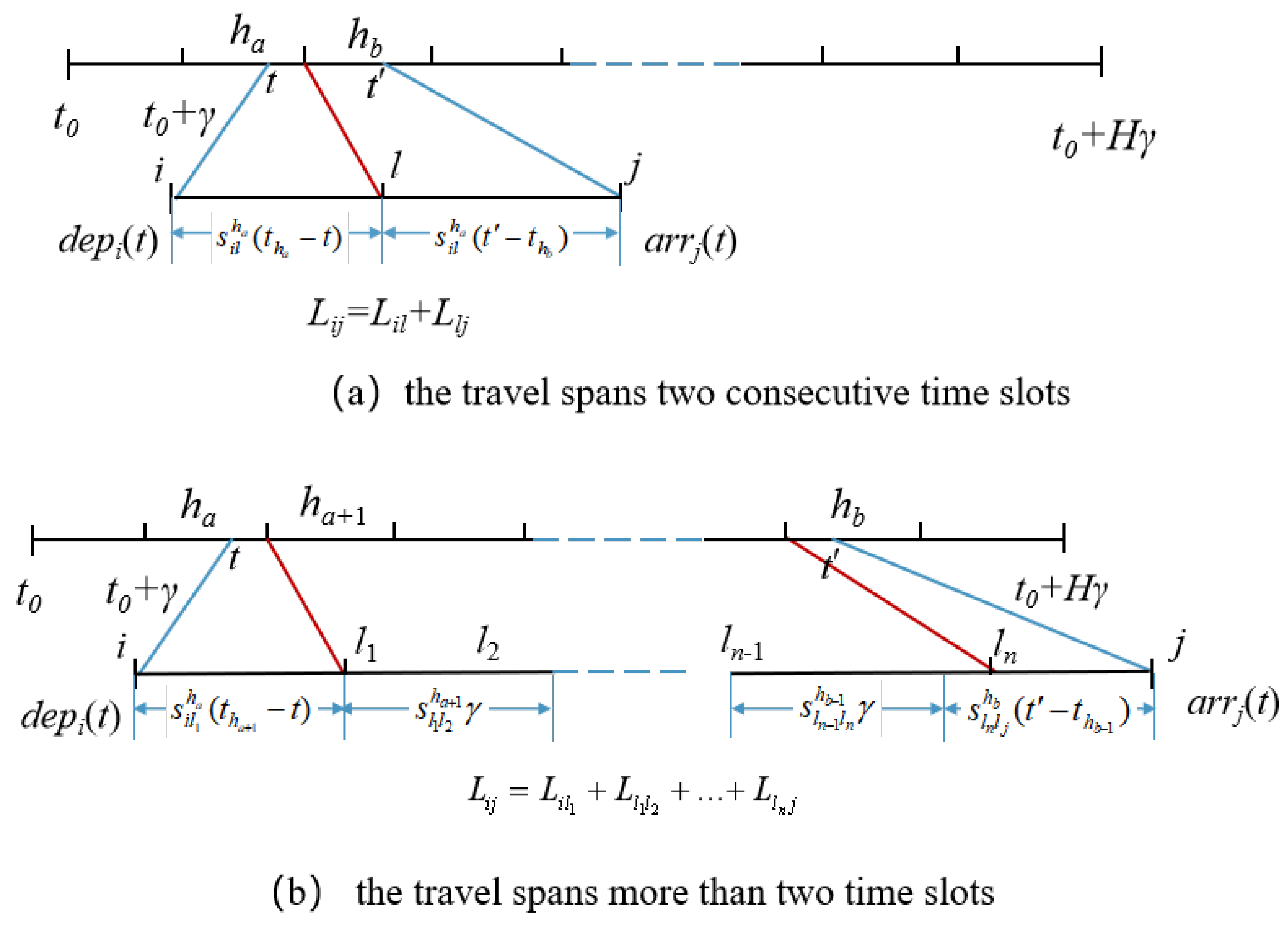
• When $h_b=h_a+1$, the travel spans two consecutive time slots. The arc $(i,j)$ is split into two segments with different speeds. The arrival time at node j can be expressed as illustrated in Figure 5a:

  $${\mathrm{arr}}_j\left(t\right)={\mathrm{arr}}_i\left(t\right)+{\displaystyle \frac{L_{il}}{v_{il}^{h_a}}}+{\displaystyle \frac{L_{lj}}{v_{lj}^{h_b}}}+s_j$$

  (3)

  where $L_{il}$ and $L_{lj}$ are the distances traveled in the first and second time slots, respectively.
• When $h_b>h_a+1$, the travel spans more than two time slots. The total travel time consists of three components: the remaining time from ${\mathrm{arr}}_i\left(t\right)$ to the end of slot $h_a$, the sum of full time slots crossed, calculated as $(h_b-h_a-1)\gamma$, and the partial time within the final slot $h_b$ until arrival at node j. The arrival time at node j is then, as illustrated in Figure 5b:

  $${\mathrm{arr}}_j\left(t\right)={\mathrm{arr}}_i\left(t\right)+{\displaystyle \frac{L_{i{l}_1}}{v_{i{l}_1}^{h_a}}}+(n-1)\gamma +{\displaystyle \frac{L_{l_{n-1}j}}{v_{l_{n-1}j}^{h_b}}}+s_j$$

  (4)
  Here, the arc $L_{ij}$ is divided into $(n+1)$ segments, as illustrated in Figure 5b.

3.3. Symbols and Parameters

We adopt the notations summarized in

Table 1. Notations for energy consumption and carbon emission model.

Sets
m	Set of depots, $m=1,2,\dots ,m$
K	Set of trucks, $K=1,2,\dots ,k$
C	Set of customers, $C=m+1,m+2,\dots ,m+c$
$C_0$	Set of starting nodes including depots and customers, $C_0=M\cup C$
$C_{+}$	Set of ending nodes including customers and depots, $C_{+}=C\cup M$
N	Set of all nodes, $N=C_0\cup C_{+}$
Parameters
$F_0$	Fuel consumption at empty load (L/100 km)
$F^{*}$	Fuel consumption at full load (L/100 km)
Q	Maximum payload capacity (kg)
$W_{ij}^k$	Load of truck k on arc $(i,j)$ (tons)
$D_{ij}$	Distance from node i to node j (km)
$d_{ij}^{k{T}_L}$	Travel distance of truck k on arc $(i,j)$ during time period $T_L$
$t_i^k$	Arrival time of truck k at customer i
$[B_i,E_i]$	Represents the time window of customer i
$T_L$	Set of working time periods, $T_L=T_1,T_2,\dots ,T_L$
$t_{ij}$	Travel time on arc $(i,j)$ (hours)
$t_{\mathrm{service}}$	Service time at node j (hours)
$p_j$	Delivery quantity at node j (kg)
$P_0$	Base refrigeration power (L/hour)
$\beta$	Cooling load coefficient (L/hour)
$P_{\mathrm{fuel}}$	Fuel price (RMB/L)
$P_{\mathrm{carbon}}$	Carbon price (RMB/kg CO2)
$P_1$	Fixed cost per vehicle (RMB/vehicle)
$P_2$	Penalty per hour of delay (RMB/hour)
${\gamma }_{\mathrm{fuel}}$	Carbon emission factor for fuel (kg CO2/L)
${\gamma }_{\mathrm{cool}}$	Carbon emission factor for refrigeration (kg CO2/L)
Variables
$x_{ij}^k\in \{0,1\}$	1 if truck k travels from node i to node j, 0 otherwise
$y_{mj}^k\in \{0,1\}$	1 if vehicle k is dispatched from depot m to serve customer j
$u_i^k$	Subtour elimination variable

to mathematically formulate the problem as an MILP model.

3.4. Objective Function

According to the studies by [39,40], the total energy consumption consists of three major components: fixed cost, driving energy consumption, and refrigeration energy consumption. Both are affected by dynamic payload variations and operational time. The corresponding carbon emission cost is computed based on the energy consumed and the carbon emission factors.

3.4.1. Fixed Cost

The fixed cost is incurred when a truck is dispatched from the depot to serve customers and is modeled as:

$$FC=P_1·\sum _{m\in M}\sum _{k\in K}\sum _{j\in C}{y}_{mj}^k$$

(5)

where $P_1$ represents the fixed dispatch cost per vehicle and K is the number of refrigerated trucks.

3.4.2. Driving Energy

According to the literature [40,41], the fuel consumption for a truck traveling from node i to node j is modeled as a linear function of payload weight:

$$F_{ij}=\left(F_0+{\displaystyle \frac{F^{*}-F_0}{Q}}·W_{ij}\right)·d_{ij}$$

(6)

Specifically, $F_0$ represents the fuel consumption per 100 km when the truck is empty (L/100 km) and $F_{*}$ represents the fuel consumption per 100 km when the truck is fully loaded (L/100 km). Q denotes the maximum payload capacity of the truck (kg), and $W_{ij}$ is the actual payload on arc $(i,j)$ (kg). The total driving energy cost, including fuel and carbon emissions, is:

$$C_{\mathrm{drive}}=\sum _{k\in K}\sum _{i\in C_0}\sum _{j\in C_{+}}{F}_{ij}^k·\left(P_{\mathrm{fuel}}+{\gamma }_{\mathrm{fuel}}·P_{\mathrm{carbon}}\right)·x_{ij}^k$$

(7)

3.4.3. Refrigeration Energy

According to the literature [39,40], the refrigeration energy depends on both travel time and service time, and linearly increases with payload weight due to thermal load:

During driving:

$$E^{\mathrm{cool}}{ij}^k=\left(P_0+\beta W_{ij}^k\right)·t_{ij}$$

(8)

During service:

$$E^{\mathrm{service}}{j}^k=(P_0+\beta (W{ij}^k-p_j))·t_{\mathrm{service}}$$

(9)

The total refrigeration energy cost including carbon emissions is:

$$C_{\mathrm{total}}^{\mathrm{cool}}=\sum _{k\in K}\sum _{i\in C_0}\sum _{j\in C_{+}}{E}^{\mathrm{cool}}{ij}^k·\left(P_{\mathrm{fuel}}+{\gamma }_{\mathrm{cool}}·P_{\mathrm{carbon}}\right)·x_{ij}^k+\sum _{k\in K}\sum _{j\in C}{E}^{\mathrm{service}}{j}^k·\left(P_{\mathrm{fuel}}+{\gamma }_{\mathrm{cool}}·P_{\mathrm{carbon}}\right)$$

(10)

3.4.4. Time Window Penalty

In cold chain logistics, the condition of products upon delivery is crucial, as it directly affects customers’ revenue, inventory management, and quality control. Therefore, both early and late arrivals reduce customer satisfaction. In this model, a penalty cost is incurred whenever a vehicle arrives outside the specified time window of a customer [42,43,44]. The penalty cost is formulated as:

$$C_{\mathrm{TW}}=P_2·\sum _{k\in K}\sum _{i\in C}max(0,B_i-A_i^k)+P_3·\sum _{k\in K}\sum _{i\in C}max(0,A_i^k-E_i)$$

(11)

where $C_{\mathrm{TW}}$ represents the total time window penalty cost, $t_i^k$ is the arrival time of vehicle k at customer iii, and $P_2$ and $P_3$ are the unit penalty costs for early and late arrivals, respectively.

3.5. Mathematical Model

The complete objective function minimizing the total operational cost is:

$$minC=FC+C_{\mathrm{drive}}+C_{\mathrm{total}}^{\mathrm{cool}}+C_{\mathrm{TW}}$$

(12)

Flow Conservation

$$\sum _{m\in M}\sum _{k\in K}\sum _{i\in C}{x}_{ij}^k=1,\forall j\in C$$

(13)

$$\sum _{j\in C}{x}_{mj}^k=\sum _{j\in C_{+}}{y}_{mj}^k,\forall m\in M,k\in K$$

(14)

$$\sum _{j\in N}{x}_{ij}^k=\sum _{j\in N}{x}_{ji}^k,\forall i\in C,k\in K$$

(15)

$$\sum _{j\in M}{x}_{ij}^k\le 1,\forall i\in C,k\in K$$

(16)

Payload Balance

$$W_{mj}^k=Q·y_{mj}^k,\forall m\in M,j\in C,k\in K$$

(17)

$$W_{jk}^k=W_{ij}^k-p_j·x_{ij}^k,\forall i\in C_0,j\in C_{+},k\in K$$

(18)

$$0\le W_{ij}^k\le Q·x_{ij}^k$$

(19)

$$D_{ij}=\sum _{T_L\in T}{d}_{ij}^{T_{L}k}{x}_{ij}^k,\forall i\in N,j\in N,k\in K$$

(20)

Time Propagation

$$t_j^k\ge (t_i^k+t_{service}+t_{ij})·x_{ij}^k,\forall i\in C_0,j\in C_{+},k\in K$$

(21)

$$t_{ij}^k=\sum _{T_L\in T}{t}_{ij}^{T_{L}k}{x}_{ij}^k,\forall i\in N,k\in K,T_L\in T$$

(22)

$$t_{ij}^{T_{L}k}=\sum _{T_L\in T}{d}_{ij}^{T_{L}k}/v_{ij}^{T_{L}k},\forall i\in N,j\in N,k\in K$$

(23)

Subtour Elimination (MTZ)

$$u_i^k-u_j^k+\left|N\right|·x_{ij}^k\le \left|N\right|-1,\forall i\in C_0,j\in C_{+},i\ne 0,j\ne 0,k\in K$$

(24)

$$1\le u_i^k\le \left|N\right|,\forall i\in C_{+},k\in K$$

(25)

Variable Domains

$$x_{ij}^k\in \{0,1\},\forall i\in C_0,j\in C_{+},k\in K$$

(26)

$$y_{mj}^k\in \{0,1\},\forall i\in C_0,j\in C_{+},k\in K$$

(27)

$$t_i^k\ge 0,W_{ij}^k\ge 0,u_i^k\ge 0,\forall (i,j)\in A,k\in K$$

(28)

The constraints (13)–(16) represent the flow balance constraints, which ensure that each customer is visited exactly once and that route continuity is maintained for each truck. The payload balance constraints (17)–(19) dynamically track the remaining load of each vehicle along its route based on customer demands. Constraint (20) represents the relationship between the segment distance and the distance traveled by the vehicle across multiple time periods. Constraint (21) represents the time relationship of the vehicle traveling from the previous node to the next node. Constraints (22) and (23) represents the relationship between travel time, travel speed, and travel distance of a vehicle within the same time period. To prevent infeasible sub-tours, the model incorporates the MTZ constraints (24) and (25). Finally, constraints (26)–(28) specify the variable domains, including binary decision variables for routing and non-negativity requirements for arrival times and payloads.

4. A TDGVRP Heuristic

4.1. Algorithm Design

In the previous section, a Mixed-Integer Programming (MIP) model for the TDGVRP was formulated, as shown in Equations (1)–(28). Essentially, TDGVRP is a generalized form of the classical VRP, which is an NP-hard problem [45,46,47]. Therefore, TDGVRP inherits this NP-hard complexity. While exact solvers like Gurobi can efficiently solve small-scale instances (e.g., fewer than 10 nodes), solving large-scale problems becomes computationally prohibitive.

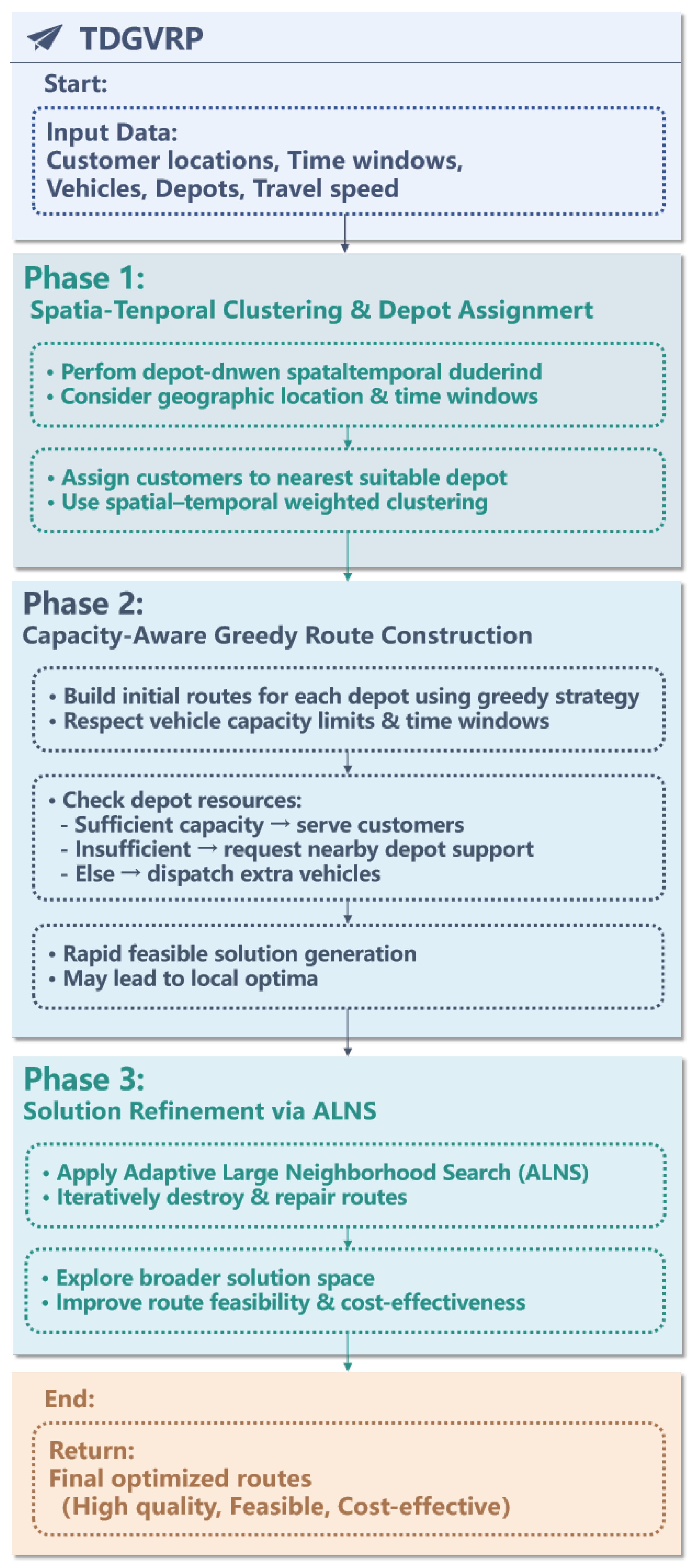
To address the complexity and scale of the TDGVRP, this study proposes a novel three-phase heuristic algorithm designed to efficiently generate high-quality solutions for large-scale instances. The algorithm comprises the following three stages (see Figure 6):

Phase 1: Spatial–Temporal Clustering and Depot Assignment. The algorithm begins by performing depot-driven spatial–temporal clustering, which jointly considers the geographic locations and time window constraints of customers. A spatial–temporal weighted clustering approach is used to assign customers to the most appropriate depot, laying the foundation for subsequent route construction.

Phase 2: Capacity-Aware Greedy Route Construction. Based on the clusters formed in Phase 1, a capacity-aware greedy algorithm is applied to construct initial truck routes for each depot. This phase takes into account vehicle capacity limitations and customer time windows. The algorithm dynamically determines whether a depot has sufficient vehicle resources to serve all assigned customers, whether support from nearby depots is required, or whether additional vehicles need to be dispatched. Although the greedy strategy enables rapid generation of feasible solutions, it may lead to suboptimal local solutions due to its heuristic nature and dependence on initial cluster quality.

Phase 3: Solution Refinement via Adaptive Large Neighborhood Search (ALNS). To overcome the limitations of the initial solution and escape local optima, the third phase integrates an Adaptive Large Neighborhood Search (ALNS) framework, as introduced by Ropke and Pisinger [48]. This phase iteratively performs destruction and repair operations to explore a broader solution space, improving route feasibility and cost-effectiveness over successive iterations.

Together, these three phases provide a scalable and effective approach to solving the TDGVRP, balancing computational efficiency and solution quality through a structured heuristic optimization pipeline.

4.2. Depot-Driven Spatial–Temporal Weighted Clustering

In cold chain logistics, customers are not only geographically dispersed but also subject to strict time window constraints. For example, certain fresh food retailers may require deliveries in the early morning (e.g., [6:00, 9:00]), while others may prefer afternoon deliveries. This dual heterogeneity in spatial locations and time requirements makes traditional clustering methods based solely on spatial distance or time windows insufficient for generating cost-effective delivery plans.

To address this, a depot-driven spatial–temporal weighted K-means clustering method is proposed. This method fully integrates customers’ spatial coordinates and time window characteristics. Centered around depots, it partitions customers into balanced spatial–temporal clusters, each served by a designated depot. This approach effectively reduces cross-region transportation costs and minimizes time window violation penalties.

For each customer i, the time window is first transformed into a time window center:

$$t{w}_i={\displaystyle \frac{a_i+e_i}{2}}$$

(29)

where $a_i$ and $e_i$ denote the earliest and latest service times for customer i, respectively. The time window center $t{w}_i$ represents the customer’s temporal service preference. For example, a customer with a time window of [8:00, 10:00] has $t{w}_i=9.0$, indicating a preference for delivery around 9:00.

To integrate spatial coordinates $(x_i,y_i)$ and the time window center $t{w}_i$ into a unified feature space, normalization is performed to map all variables into the [0, 1] range:

$$x_{\mathrm{norm},i}={\displaystyle \frac{x_i-x_{min}}{x_{max}-x_{min}}},y_{\mathrm{norm},i}={\displaystyle \frac{y_i-y_{min}}{y_{max}-y_{min}}}$$

(30)

$$t{w}_{\mathrm{norm},i}={\displaystyle \frac{t{w}_i-t{w}_{min}}{t{w}_{max}-t{w}_{min}}}$$

(31)

The normalized feature vector for each customer is defined as:

$$v_i=\left(x_{\mathrm{norm},i},y_{\mathrm{norm},i},t{w}_{\mathrm{norm},i}\right)$$

(32)

A spatial–temporal weighted distance between customer i and depot m is then computed as:

$$D_{im}=\alpha ·\sqrt{{(x_{\mathrm{norm},i}-x_m)}^2+{(y_{\mathrm{norm},i}-y_m)}^2}+(1-\alpha )·|t{w}_{\mathrm{norm},i}-t{w}_m|$$

(33)

where $\alpha \in [0,1]$ is a user-defined weighting coefficient that balances the importance between spatial proximity and time window similarity.

Customers are assigned to the depot with the minimum weighted distance:

$$C_m=\left\{i\right|D_{im}=\underset{j\in M}{min}{D}_{ij}\}$$

(34)

At this stage, each customer is associated with its nearest depot in terms of spatial–temporal similarity. The depot functions not only as a spatial center but also as a coordinator of time window compatibility.

Each cluster center is then updated based on the average of its assigned customers:

$$c_m={\displaystyle \frac{1}{|C_m|}}\sum _{i\in C_m}{\mathbf{v}}_i$$

(35)

This updated center reflects the average spatial and temporal characteristics of the customers within the cluster. The algorithm checks whether or not the customer assignments remain unchanged compared to the previous iteration. If stable, or if the maximum number of iterations is reached, the clustering process terminates. Otherwise, the algorithm returns to the distance calculation step and continues iterating.

The proposed clustering method efficiently balances spatial proximity and time window compatibility. It produces depot-specific customer clusters, which significantly improve the quality of initial solutions for the MDVRPTW.

4.3. Capacity-Aware Spatial–Temporal Greedy Route Construction

After completing the spatial–temporal weighted clustering, each depot m is assigned a relatively independent customer subset $C_m$. However, cold chain logistics not only requires consideration of geographical proximity and time windows but also imposes strict constraints on vehicle capacity. In multi-depot, multi-vehicle distribution scenarios, efficient capacity allocation is critical to minimizing total logistics costs.

To address this, a capacity-aware spatial–temporal greedy route construction Algorithm 1 is proposed. This algorithm jointly considers spatial distance, time window constraints, vehicle capacity, and cost factors, aiming to efficiently construct initial truck routes with minimized travel distance, time window violations, and fixed vehicle costs.

For each depot m and its associated customer set $C_m$, a spatial–temporal priority score is computed for each customer $i\in C_m$:

$${\mathrm{Priority}}_i=\alpha ·{\mathrm{SpatialDistance}}_{Depot,i}+(1-\alpha )·{\mathrm{TimeUrgency}}_i$$

(36)

where $\alpha$ is a weighting coefficient balancing spatial distance and time urgency. Customers that are geographically closer to the depot and have tighter time windows are prioritized.

Algorithm 1: Capacity-Aware Greedy Route Construction with Multi-Depot

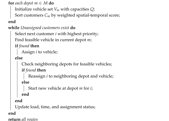
A vehicle pool is initialized for each depot m. Customers are sorted in ascending order of their priority scores. Starting from the depot, the algorithm iteratively attempts to add customers to the current truck route while satisfying two conditions: (1) the remaining vehicle capacity must be greater than or equal to the customer’s demand, and (2) the arrival time plus service time must satisfy the customer’s time window constraints.

If no vehicle within the current depot can serve customer i, the algorithm checks whether or not neighboring depots have vehicles with sufficient remaining capacity and feasible time windows. If such vehicles exist, customer i is dynamically reassigned to that depot. If none of the existing vehicles can accommodate customer i, a new vehicle is instantiated at the current depot to serve the customer, incurring additional fixed costs, energy consumption, and carbon emissions.

After each customer insertion, the algorithm updates the remaining capacity and arrival times for the entire route. This process continues until all customers have been successfully assigned to feasible routes.

4.4. ALNS

The initial solutions for the TDGVRP heavily rely on the quality of the depot-based mVRP clustering. Consequently, the performance of the routing solution can be significantly influenced by the clustering results. To further improve the solution quality, this study introduces an ALNS metaheuristic tailored for the TDGVRP.

ALNS, initially proposed by Ropke and Pisinger [48], extends the Large Neighborhood Search (LNS) framework introduced by Shaw [49]. ALNS has been widely recognized for its excellent performance on the VRP and its variants. The core idea of ALNS is to iteratively destroy and repair parts of the current solution using a set of different operators. The choice of operators is guided by an adaptive, score-based roulette wheel selection mechanism that favors operators with better historical performance.

Let $H=\{h_1,h_2,\dots ,h_k\}$ represent the set of all available operators, including both removal and repair strategies. Each operator $h_j$ is associated with a weight $w_j$, which determines its selection probability as follows:

$$P\left(h_j\right)={\displaystyle \frac{w_j}{{\sum }_{i=1}^k{w}_i}}$$

(37)

Initially, all operators are assigned equal weights. As the search progresses, these weights are adaptively adjusted based on the operators’ performances. The scoring mechanism rewards operators under three conditions $({\sigma }_1,{\sigma }_2,{\sigma }_3)$, as summarized in

Table 2. Score adjustment parameters.

Condition	Description
${\sigma }_1$	The removal–insertion operation produces a new global best solution.
${\sigma }_2$	The operation results in a solution better than the current one.
${\sigma }_3$	The operation yields a solution accepted by the acceptance criterion but worse than the current one.

.

Every $\Delta$ iterations, the weights are updated using the accumulated scores. Let $w_i$ denote the weight of operator i at the current update, and ${\varphi }_i$ represent its accumulated score. The weight update rule is:

$$w_i=w_i·(1-\rho )+\rho ·{\varphi }_i$$

(38)

where $\rho \in [0,1]$ is a reaction factor that controls how strongly the recent performance affects the updated weight. Typical values for $\rho$ range between 0.1 and 0.3.

During each iteration, the algorithm selects one removal operator and one insertion operator using the roulette wheel selection based on $P\left(h_j\right)$. The removal operator destructs part of the current solution by eliminating customers or routes, while the insertion operator repairs the solution by reinserting customers into feasible routes. The adaptive mechanism ensures that operators with better historical performance are more likely to be selected, enhancing the search efficiency and solution quality.

4.4.1. Destruction Operators

To enhance solution diversity and facilitate effective exploration, this study designs multiple destruction (removal) operators, including both random-based and cost-driven strategies. Each operator can be executed in two modes: (1) local mode, which restricts the removal within customers assigned to a single depot, and (2) global mode, which disregards the current depot assignment and allows removal across all depots.

(1)

Random Removal

Random removal is designed to introduce stochasticity into the search process. Two types of random removal operators are considered:

• Customer-Based Random Removal: Randomly select a number of customers p from the target set. In the local mode, customers are randomly selected within a single depot; in the global mode, customers are selected from the entire customer set regardless of depot assignment.
• Route-Based Random Removal: Randomly select one truck route, then remove a consecutive subsequence of customers of length L from that route. For example, given the route $(\mathrm{Depot},i_1,i_2,i_3,...,i_6,\mathrm{Depot})$, a possible removal could be $(i_2,i_3,i_4)$. This strategy effectively disrupts spatial structures and enables more flexible route reconstructions.

To prevent excessive or insufficient removal, the number of customers to be removed is dynamically adjusted within predefined bounds. The update rule is:

$$D_{\mathrm{select}}(t+1)=min\left(D_{max},max\left(D_{min},D_{\mathrm{select}}\left(t\right)+\Delta D\left(t\right)\right)\right)$$

(39)

where $D_{min}$ and $D_{max}$ represent the lower and upper bounds of removal quantity, ensuring a balanced trade-off between exploration and solution stability. $\Delta D\left(t\right)$ is the adjustment term at iteration t.

After each removal operation, the remaining payload and time information of all affected routes are updated accordingly to maintain feasibility for subsequent repair.

(2)

Worst Removal

This operator removes the customers that contribute most negatively to the objective function. The cost contribution of customer i is defined as:

$${\mathrm{Cos}\mathrm{t}}_i={\lambda }_1·\Delta d_{ijk}+{\lambda }_2·{\mathrm{TimePenalty}}_i+{\lambda }_3·{\mathrm{RefrigerationCost}}_i$$

(40)

Customers with the highest ${\mathrm{Cos}\mathrm{t}}_i$ values are prioritized for removal. This operator is particularly effective in eliminating bottleneck customers that degrade solution quality.

(3)

Time-Window-Based Removal

This operator targets customers with significant time window violations, either arriving too early or too late. Customers with the largest deviations from their allowed time windows are removed first. This removal strategy is designed to improve the overall temporal feasibility of the solution.

4.4.2. Repair Operators

The objective of the repair operators is to effectively reintegrate the removed customers into the existing routes or create new routes when necessary, ensuring solution feasibility while minimizing the total cost.

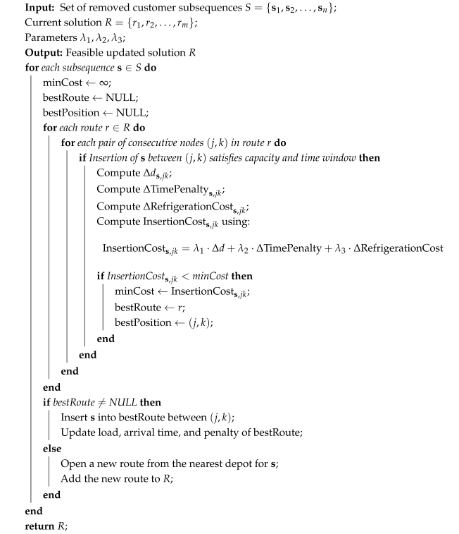
Unlike traditional methods, the proposed insertion strategy allows cross-depot and cross-vehicle insertions. For each removed customer i, Algorithm 2 evaluates all possible insertion positions across all available routes and depots.

Algorithm 2: Repair Operator with Capacity and Time Constraints

The insertion cost of placing a customer subsequence $\mathbf{s}=\{i_1,i_2,\dots ,i_p\}$ (or a customer i) between nodes $(j,k)$ in a route is defined as:

$${\mathrm{InsertionCost}}_{\mathbf{s},jk}={\lambda }_1·\Delta d_{\mathbf{s},jk}+{\lambda }_2·\Delta {\mathrm{TimePenalty}}_{\mathbf{s},jk}+{\lambda }_3·\Delta {\mathrm{RefrigerationCost}}_{\mathbf{s},jk}$$

(41)

where:

• $\Delta d_{\mathbf{s},jk}$ is the additional distance cost caused by inserting $\mathbf{s}$ between $(j,k)$:

  $$\Delta d_{\mathbf{s},jk}=d_{j,i_1}+\sum _{t=1}^{p-1}{d}_{i_t,i_{t+1}}+d_{i_p,k}-d_{j,k}$$

  (42)
• $\Delta {\mathrm{TimePenalty}}_{\mathbf{s},jk}$ is the change in time window penalty due to insertion.
• $\Delta {\mathrm{RefrigerationCost}}_{\mathbf{s},jk}$ is the change in refrigeration cost, proportional to the increase in travel time.

We first attempt to insert the customer subsequence $\mathbf{s}$—which can represent either a single customer i or a sequence of consecutive customers—into any feasible position within the current depot’s routes. The insertion prioritizes the position with the minimal total cost while strictly satisfying both the vehicle’s capacity and the customer’s time window constraints. If no feasible insertion is found within the current depot, the algorithm extends the search to the k nearest neighboring depots based on spatial proximity, thereby maintaining a balance between solution quality and computational efficiency. If all existing routes fail to accommodate the subsequence $\mathbf{s}$ due to capacity violations or time infeasibility, a new route is created at the current depot, which incurs a fixed vehicle cost.

To improve computational efficiency, the algorithm performs preliminary feasibility checks before calculating detailed insertion costs. It first verifies whether or not the remaining capacity of a candidate route satisfies the constraint:

$$W_{jk}+q_{\mathbf{s}}\le Q$$

(43)

If not, the insertion attempt at this position is immediately discarded. Additionally, the algorithm estimates the expected arrival time at the subsequence $\mathbf{s}$ when placed between nodes $(j,k)$; if the arrival time falls outside the valid time window $[T^{\mathrm{start}}\mathbf{s},T^{\mathrm{end}}\mathbf{s}]$, the insertion is rejected. Upon a successful insertion, the algorithm updates the remaining vehicle capacity, recalculates the arrival and departure times for all affected nodes, and adjusts the time window penalties and refrigeration costs accordingly.

5. Computation and Experiments

The proposed algorithm for solving the TDGVRP was implemented in Python 3.9.13, and all computational experiments were conducted on a machine equipped with an AMD Ryzen 7 6800H 3.20 GHz processor and 16 GB of RAM. Gurobi was employed as the linear programming solver, and a time limit of 3600 s was set for all tests.

5.1. Instances and Parameter Settings

In this section, we evaluate the performance of the proposed algorithm on small-, medium-, and large-scale instances, and analyze carbon emissions through a real-world case study.

For dataset 1, we utilized data from the Solomon benchmark set. Given that the C-type instances in the dataset provide relatively long service times per customer—simulating long-haul transportation scenarios—we only selected the R-type and RC-type instances for our experiments. Two sets of instances were generated based on the TDGVRP model, namely the R101-R110 and RC101-RC108 instances.

Dataset 2 is derived from the operational data of four cold-chain logistics companies located in Chengdu, China [50]. These companies deliver the same frozen products to customers situated in downtown Chengdu. Each company operates independently. Due to the use of single-distribution models, these companies are required to make significant upfront investments in warehouses, resulting in high distribution costs and relatively low long-term profits. Additionally, because of the uncertainty in specific cold-chain products and market demands, even though customer demand per delivery is relatively low, delivery frequency remains high. Thus, these companies must distribute small quantities of cold-chain products multiple times each day. The characteristics of the empirical data used in this study realistically reflect the operational environment of the cold-chain logistics sector. Therefore, the selected data can be regarded as representative of China’s cold-chain logistics industry and its distinctive features.

The case study data were sourced from the research of Liu (2020) [50], which focused on joint distribution strategies for minimizing the total distribution cost of cold-chain products.

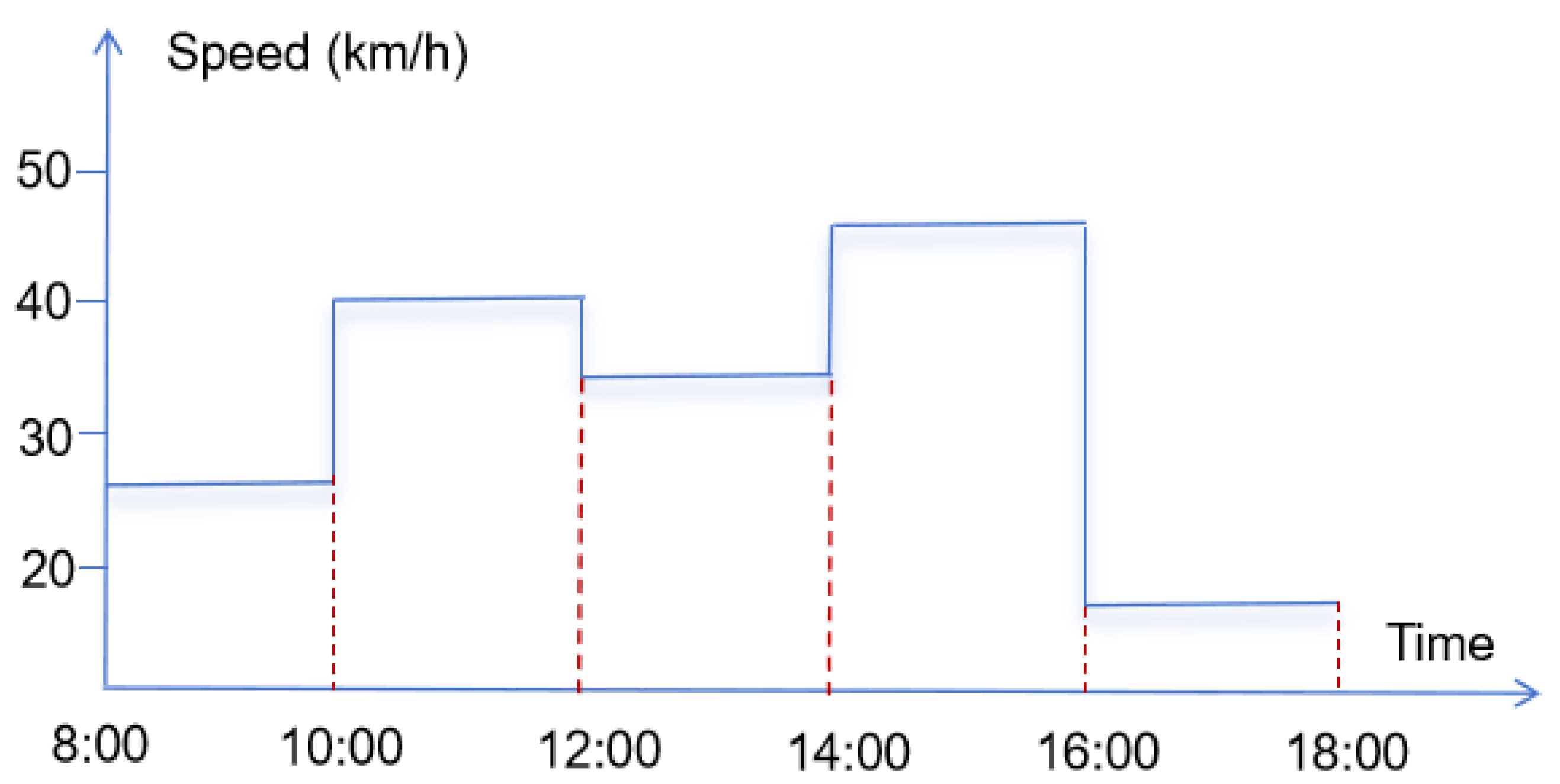
However, that study overlooked the impact of traffic conditions during transportation. Therefore, this study incorporates time-varying speed profiles under the carbon trading mechanism, taking into account the actual traffic conditions in Chengdu [51,52]. The detailed speed profiles are presented in

Table 3. Traffic time period forecast and analysis in Chengdu.

Time Period	Speed (km/h)	Traffic Condition
08:00–10:00	26	Moderate Congestion
10:00–12:00	40	Light Congestion
12:00–14:00	35	Slow Moving
14:00–16:00	45	Basically Smooth
16:00–18:00	18.5	Severe Congestion

and Figure 7. Meanwhile, the parameter settings in this study are based on standard procedures established by Wang, Chen, and Liu [27,43,50], as summarized in

Table 4. Parameter settings in the case study.

Symbols	Description	Unit	Value
m	Number of depots	none	4
n	Number of customers (all)	none	28
$P_1$	Fixed cost of each vehicle	RMB/car	200
$P_{fuel}$	Fuel price per unit	RMB/L	6.68
$F_{wait}$	Waiting cost for early arrival	RMB/h	50
$F_{late}$	Penalty cost for late arrival	RMB/h	50
$P_0$	Base refrigeration power	L/h	2
$P_{carbon}$	Carbon price	RMB/kg	0.25
$t_{service}$	Service time	h	0.15
${\beta }_1$	Cooling load coefficient during transport	L/h/kg	0.2
${\beta }_2$	Cooling load coefficient during unloading	L/h/kg	0.25
$F_0$	Fuel consumption (empty, per km)	L/km	0.165
$F^{*}$	Fuel consumption (full load, per km)	L/km	0.377
Q	Truck maximum capacity	kg	2000
${\gamma }_{\mathrm{fuel}}$	Carbon emission factor for fuel	kg/L	2.68
${\gamma }_{\mathrm{cool}}$	Carbon emission factor for refrigeration	kg/L	2.68

.

5.2. Computational Results of Experiment 1

Since no benchmark solutions are available for the TDGVRP problem, this study compares the proposed Three-Phase Heuristic Algorithm (TPH) with the exact solutions obtained using the Gurobi solver, as well as with the Genetic Algorithm (GA). The Solomon R101–R110 and RC101-RC110 instances were selected for evaluation, with the truck capacity fixed at 50. Both the TPH and the GA were run 10 times, and the best solution and the average solution were recorded.

Table 5. Comparison between MILP, TPH, and GA use R-type instances.

Ins.	MILP	TPH					GA
		Best	Gap (%)	Avg	Gap (%)	Time (s)	Best	Gap (%)	Avg	Gap (%)	Time (s)
R101_15	296.66	296.66	0.00%	301.83	1.71%	22.38	304.00	2.41%	317.98	6.70%	26.65
R102_15	281.99	282.00	0.00%	282.19	0.07%	18.12	282.39	0.14%	285.46	1.22%	18.23
R103_15	282.39	282.39	0.00%	289.83	2.57%	17.86	292.92	3.60%	308.45	8.43%	18.41
R104_15	242.48	242.48	0.00%	253.24	4.25%	17.85	256.62	5.51%	260.99	7.09%	17.66
R105_15	297.26	297.26	0.00%	312.83	4.98%	18.17	319.97	7.10%	327.54	9.25%	18.38
R106_15	256.25	256.25	0.00%	265.48	3.48%	17.61	282.82	9.40%	291.47	12.08%	18.415
R107_15	296.97	296.97	0.00%	307.68	3.48%	17.53	306.01	2.95%	313.65	5.32%	17.69
R108_15	240.91	240.91	0.00%	252.75	4.68%	18.18	253.02	4.79%	263.67	8.63%	18.45
R109_15	329.83	329.83	0.00%	345.42	4.51%	18.22	348.98	5.49%	350.40	5.87%	18.35
R110_15	271.76	271.76	0.00%	281.09	3.32%	20.10	289.92	6.27%	304.28	10.69%	19.73
Avg			0.00%		3.31%	18.602		4.47%		7.53%	19.1965
R101_30	627.28	629.19	0.30%	631.83	0.72%	46.44	641.09	2.15%	649.20	3.38%	45.97
R102_30	633.41	634.46	0.17%	645.88	1.93%	38.63	651.59	2.79%	657.30	3.63%	37.55
R103_30	566.96	565.11	−0.33%	574.46	1.31%	37.29	583.80	2.89%	594.46	4.63%	36.88
R104_30	463.99	463.96	−0.01%	491.34	5.57%	36.60	482.92	3.92%	511.91	9.36%	36.29
R105_30	519.02	518.72	−0.06%	547.85	5.26%	37.91	556.90	6.80%	566.83	8.44%	37.33
R106_30	610.57	610.59	0.00%	615.98	0.88%	37.20	613.47	0.47%	637.32	4.20%	37.39
R107_30	554.97	555.04	0.01%	573.77	3.28%	36.23	586.87	5.44%	599.09	7.36%	36.21
R108_30	438.53	439.34	0.18%	469.94	6.68%	36.97	477.13	8.09%	481.28	8.88%	36.17
R109_30	588.06	587.39	−0.11%	610.60	3.69%	42.49	611.07	3.76%	629.20	6.54%	43.56
R110_30	642.13	641.42	−0.11%	674.06	4.74%	40.42	692.02	7.21%	706.45	9.10%	40.44
Avg			0.01%		3.41%	39.018		4.35%		6.55%	38.779
R101_50	1169.13	1167.07	−0.18%	1212.60	3.58%	66.61	1234.45	5.29%	1275.03	8.31%	67.16
R102_50	1054.42	1051.84	−0.25%	1109.46	4.96%	62.14	1094.51	3.66%	1147.84	8.14%	62.53
R103_50	1028.82	1025.27	−0.35%	1038.56	0.94%	61.27	1051.17	2.13%	1094.51	6.00%	61.04
R104_50	710.29	708.61	−0.24%	723.15	1.78%	59.29	739.92	4.00%	730.75	2.80%	61.55
R105_50	1148.86	1125.71	−2.06%	1181.88	2.79%	61.84	1195.95	3.94%	1213.11	5.30%	61.59
R106_50	1078.48	1062.59	−1.50%	1115.98	3.36%	60.18	1102.24	2.16%	1136.54	5.11%	61.44
R107_50	953.56	950.97	−0.27%	955.54	0.21%	60.23	983.87	3.08%	976.77	2.38%	59.965
R108_50	1152.63	1140.17	−1.09%	1165.09	1.07%	65.36	1188.55	3.02%	1180.68	2.38%	64.68
R109_50	1150.62	1130.23	−1.80%	1171.01	1.74%	65.98	1182.86	2.73%	1194.34	3.66%	65.75
R110_50	1083.60	1038.52	−4.34%	1128.68	3.99%	64.64	1131.16	4.20%	1151.62	5.91%	65.13
Avg			−1.21%		2.44%	62.754		3.42%		5.00%	63.0835

and

Table 6. Comparison between MILP, TPH, and GA used RC-type instances.

Ins.	MILP	TPH					GA
		Best	Gap (%)	Avg	Gap (%)	Time (s)	Best	Gap (%)	Avg	Gap (%)	Time (s)
RC101_15	350.98	350.98	0.00%	352.53	0.44%	22.93	351.02025	0.01%	353.6725625	0.76%	22.97
RC102_15	338.60	338.60	0.00%	342.16	1.04%	20.25	342.85	1.24%	345.13	1.89%	22.44
RC103_15	337.13	337.13	0.00%	339.39	0.67%	21.63	339.82	0.79%	342.91	1.69%	22.41
RC104_15	265.98	265.98	0.00%	271.36	1.98%	22.81	266.74	0.28%	284.69	6.57%	21.98
RC105_15	345.57	345.68	0.03%	348.16	0.75%	21.90	347.31	0.50%	350.61	1.44%	22.45
RC106_15	350.98	350.98	0.00%	359.00	2.23%	25.99	356.52	1.55%	362.22	3.10%	24.69
RC107_15	311.69	311.69	0.00%	322.19	3.26%	25.42	328.68	5.17%	333.13	6.44%	25.16
RC108_15	291.01	291.27	0.09%	296.26	1.77%	24.89	292.73	0.59%	300.57	3.18%	24.09
Avg			0.02%		1.52%	23.23		1.27%		3.13%	23.27
RC101_30	748.60	748.59	0.00%	755.55	0.92%	53.68	768.12	2.54%	810.91	7.68%	53.36
RC102_30	798.93	798.66	−0.03%	818.65	2.41%	45.90	820.43	2.62%	836.20	4.46%	44.74
RC103_30	613.11	613.49	0.06%	629.06	2.54%	45.48	624.63	1.84%	635.77	3.56%	45.55
RC104_30	695.65	694.77	−0.13%	697.28	0.23%	51.09	699.80	0.59%	711.03	2.16%	52.09
RC105_30	832.21	831.98	−0.03%	864.69	3.76%	55.87	863.26	3.60%	871.65	4.52%	55.49
RC106_30	826.91	826.47	−0.05%	831.31	0.53%	59.66	829.70	0.34%	835.76	1.06%	60.03
RC107_30	711.55	711.14	−0.06%	725.21	1.88%	55.22	722.23	1.48%	738.45	3.64%	54.57
RC108_30	750.00	750.00	0.00%	758.81	1.16%	54.57	769.49	2.53%	771.42	2.78%	55.98
Avg			−0.03%		1.68%	52.73		1.94%		3.73%	52.73
RC101_50	1578.99	1580.93	0.12%	1606.00	1.68%	66.88	1651.41	4.39%	1643.77	3.94%	67.03
RC102_50	1451.57	1450.79	−0.05%	1495.67	2.95%	76.17	1518.15	4.39%	1537.30	5.58%	77.49
RC103_50	1272.27	1272.69	0.03%	1307.03	2.66%	87.68	1296.28	1.85%	1330.95	4.41%	86.42
RC104_50	1213.15	1211.47	−0.14%	1252.80	3.16%	89.31	1263.32	3.97%	1323.42	8.33%	88.44
RC105_50	1400.57	1398.07	−0.18%	1410.17	0.68%	90.36	1426.16	1.79%	1438.14	2.61%	89.44
RC106_50	1397.68	1391.15	−0.47%	1416.18	1.31%	95.45	1422.21	1.72%	1428.54	2.16%	94.92
RC107_50	1303.16	1303.04	−0.01%	1312.41	0.70%	94.59	1319.20	1.22%	1328.73	1.92%	94.78
RC108_50	1227.49	1225.91	−0.13%	1250.87	1.87%	95.80	1259.36	2.53%	1279.15	4.04%	95.04
Avg			−0.10%		1.88%	87.28		2.73%		4.12%	86.95

present the results for instances of size 15, 30, and 50. The column MILP represents the best solution (denoted as $Best$) obtained from the Gurobi solver. The columns labeled Best and Avg correspond to the best and average solutions from the respective heuristic methods. The column Gap (%) represents the percentage deviation of the best solution from the MILP result, and Time(s) refers to the average computation time.

To comprehensively evaluate the performance of the proposed TPH algorithm, comparisons are made across three aspects: solution quality, computation time, and algorithm adaptability.

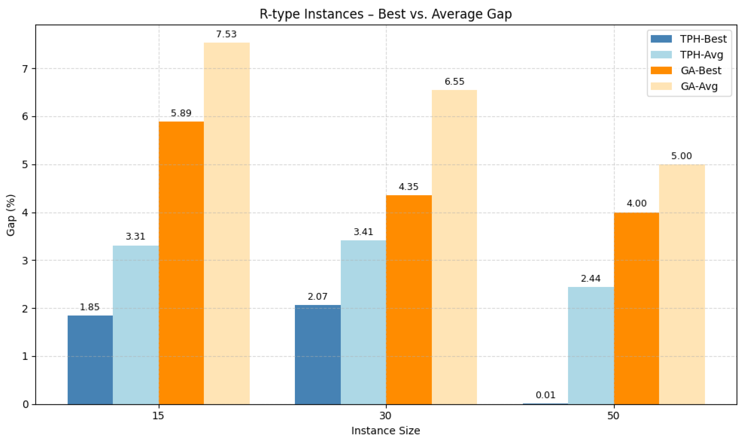
1. Solution Quality (Best and Average Performance). In the R-type instances (Figure 8), the TPH algorithm yields best solution gaps in the range of $[-1.21\%,0.01\%]$ relative to the MILP results, with an average gap of only 2.44%. For several 50-customer cases, TPH even outperforms the MILP optimal solution, demonstrating strong local search and route reconstruction capability. Compared with the GA, the TPH achieves better best solutions by over 1.0% on average, especially in medium- and large-scale instances (30 and 50 customers), indicating superior solution stability and robustness.

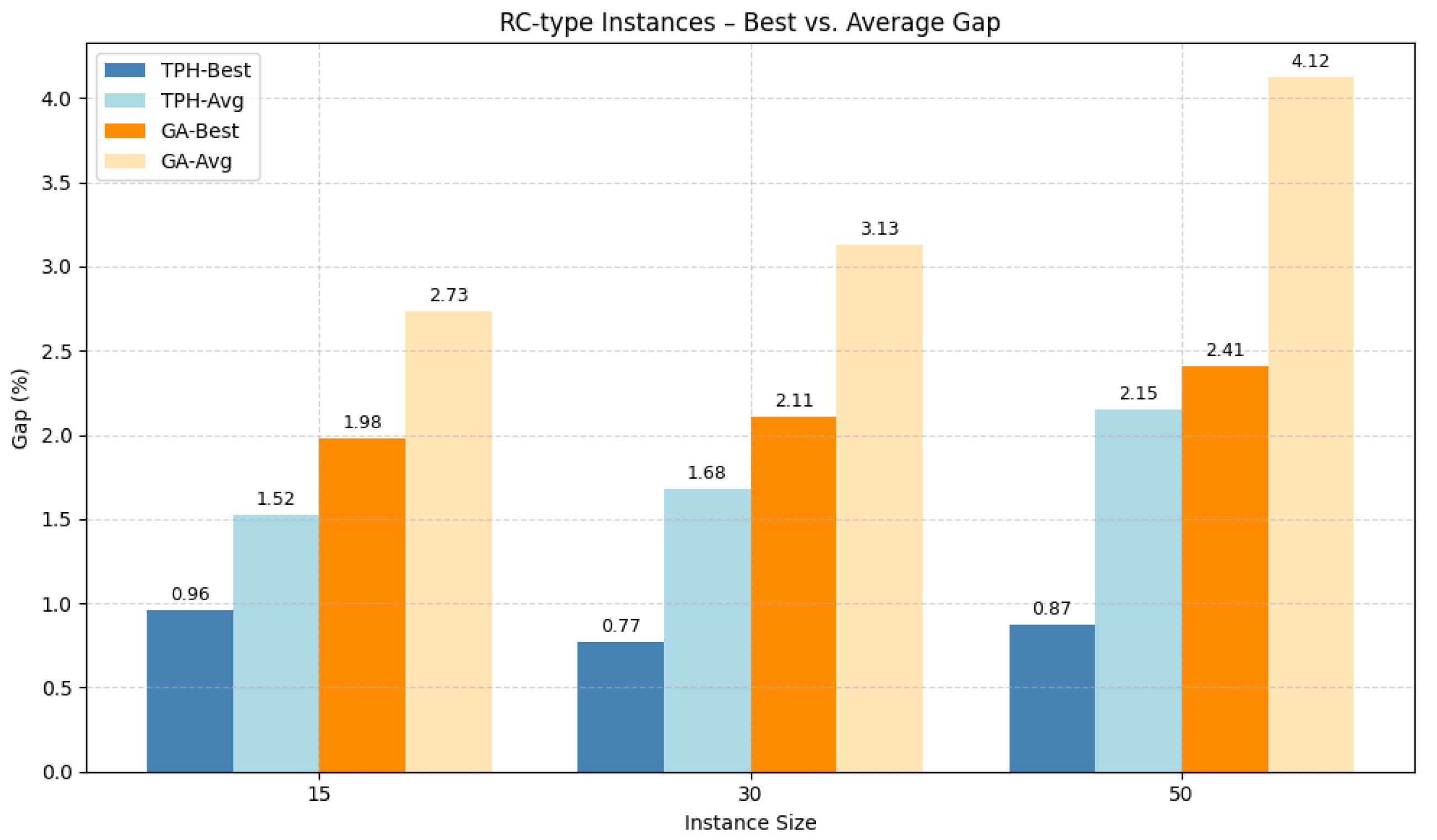
For the RC-type instances (Figure 9), which involve more complex customer distributions and tighter time windows, TPH maintains competitive performance with an average gap of 1.88%, clearly outperforming the GA’s average gap of 4.12%. In many cases, the best solutions found by TPH are very close to or even better than the lower bounds provided by Gurobi, confirming its strength under complex constraints.

2. Computation Time. In terms of runtime, the TPH algorithm averages around 60 s across all instance sizes—significantly faster than Gurobi, which often requires over 3600 s for large-scale MILP problems. Compared with GA, TPH achieves comparable or better runtimes, and in some cases it is even faster (see Time(s) column). This efficiency is especially beneficial for cold-chain logistics systems requiring real-time or near-real-time decision-making.

3. Overall Assessment and Applicability. In summary, the proposed TPH algorithm balances high solution quality with computational efficiency, making it particularly suitable for large-scale and constraint-intensive problems such as cold-chain logistics. Compared with the GA, TPH offers better solution stability and faster convergence. Its modular and flexible architecture also allows integration with real-world factors such as traffic dynamics and carbon pricing mechanisms, enhancing its engineering practicality and extensibility.

Therefore, the three-phase heuristic proposed in this study demonstrates strong empirical performance and broad application potential for solving a multi-depot, GVRP under time-window constraints.

5.3. Computational Results of Experiment 2

To evaluate the comparative performance of single-mode and joint-mode distribution strategies under realistic traffic conditions, this study adopts benchmark data from [50] and incorporates time-varying speed profiles based on actual traffic patterns in Chengdu city. A carbon pricing mechanism is implemented at a rate of 0.25 per kilogram of CO₂, and each delivery model is solved through 10 repeated runs. The optimal results are summarized in

Table 7. The comparison between the single and joint distribution mode.

Mode	Total Costs (RMB)	Carbon Costs (RMB)	Fleet Size
Single	3051.37	52.71	12
Joint	2666.20	40.52	9
Rate of decline	14.4%	23.12%	25%

. The experimental findings clearly demonstrate the superior performance of the joint distribution model across multiple dimensions. Economically, joint delivery reduces total operational costs by 14.4%, thus alleviating the financial burden on cold chain logistics providers. From an environmental perspective, carbon-related costs are decreased by 23.12%, indicating the model’s strong potential for supporting carbon neutrality goals. Moreover, the joint mode leads to a 25% reduction in fleet size, reflecting enhanced vehicle utilization and resource efficiency.

In conclusion, the joint distribution model achieves a dual objective of economic efficiency and environmental sustainability. It offers significant synergetic advantages and practical applicability, particularly in cold chain logistics scenarios characterized by high delivery time sensitivity and energy consumption. This highlights its promising value for broader implementation in sustainable logistics systems.

5.4. Sensitivity Analysis of Experiment 1

The sensitivity analysis of Three-Phase Heuristic (TPH) algorithm performance was conducted based on the detailed results from R-type and RC-type instances with varying sizes (15, 30, and 50 customers), as shown in Table 5 and Table 6.

The TPH algorithm consistently achieved high-quality solutions across all problem scales. For R-type instances, the average optimality gap relative to MILP decreased slightly from 3.31% for 15-customer cases to 2.44% for 50-customer cases, indicating that the algorithm scales well with problem size and even improves solution quality for larger instances. Moreover, the computation time increased moderately from around 18 s (15 customers) to about 63 s (50 customers), demonstrating efficient scalability. Similar trends were observed in the RC-type instances, where the average gap remained low (1.52% for 15 customers, 1.88% for 50 customers), while the computation time increased reasonably from 23 s to 87 s. These results confirm TPH’s robustness and effectiveness for both small- and large-scale scenarios.

Comparing R-type and RC-type instances reveals that TPH performs slightly better on RC-type instances, which feature more complex customer distributions and tighter time windows. The average optimality gaps for RC-type instances were generally smaller or comparable to R-type, e.g., 1.52% vs. 3.31% at 15 customers, and 1.88% vs. 2.44% at 50 customers. This suggests the heuristic’s ability to effectively manage complex temporal and spatial constraints without significant loss of solution quality.

The average gaps for TPH are consistently close to the best solution gaps across all instances, with differences generally within 1–3%, reflecting stable solution quality over multiple runs. In contrast, GA exhibits larger gaps and greater variability between best and average solutions, especially on larger instances, indicating TPH’s superior robustness and convergence reliability.

TPH maintains a favorable balance between solution quality and runtime. While MILP requires significantly longer computational times (not listed but known to be several orders of magnitude higher), TPH’s runtimes remain practical (under two minutes for 50-customer problems). Compared to GA, TPH often achieves better solution quality with comparable or less computation time, confirming its suitability for real-time or near-real-time cold chain logistics applications.

The sensitivity analysis based on varying instance sizes and types validates that the proposed TPH algorithm is scalable, robust to problem complexity, and provides consistent high-quality solutions efficiently. These characteristics make it well-suited for practical large-scale cold chain routing problems involving complex constraints.

5.5. Sensitivity Analysis of Experiment 2

(1)

Analysis of the Impact of Carbon Pricing

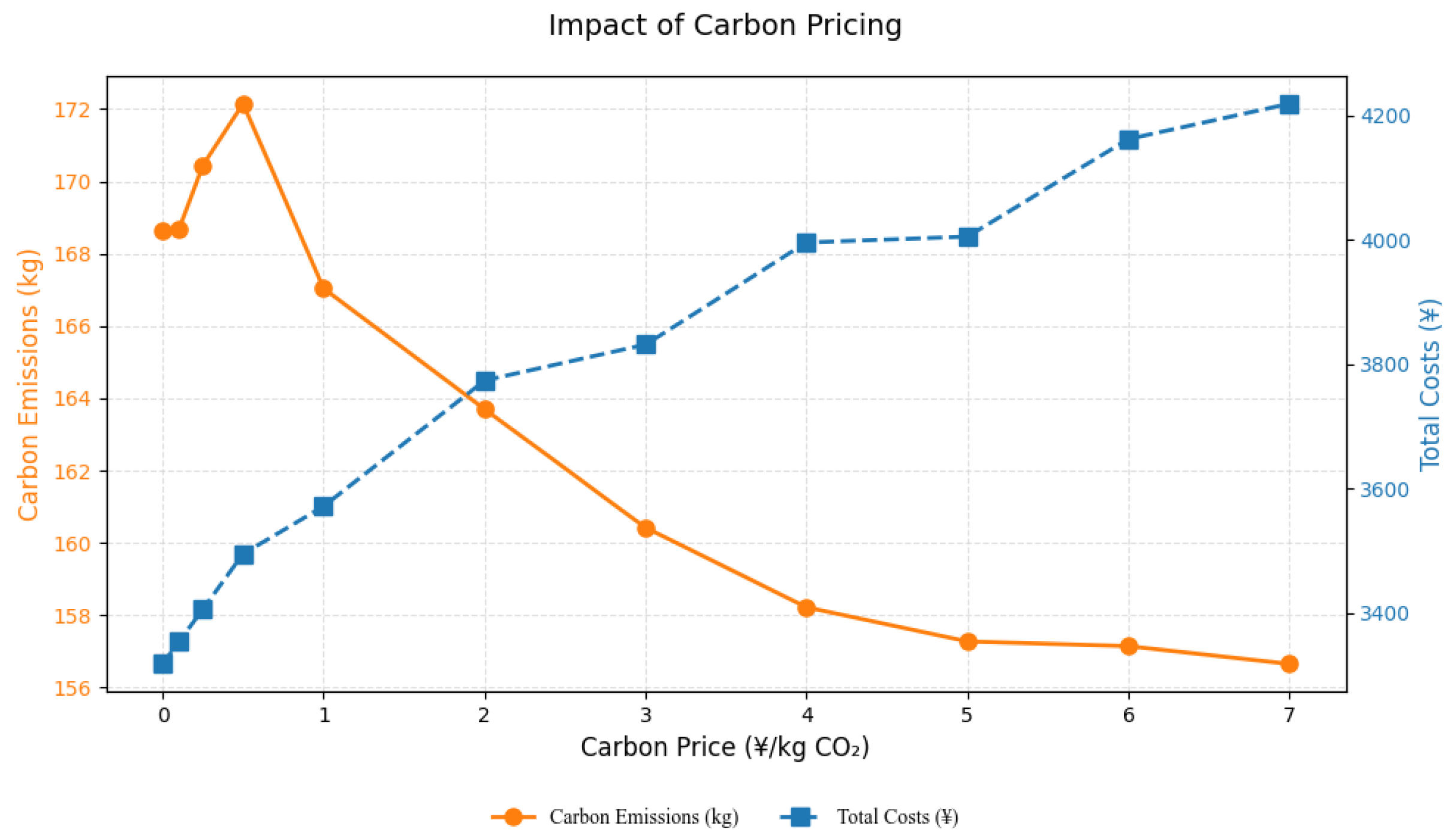
In the previous section, we analyzed joint distribution using the current market average carbon price (0.25 RMB/kg CO₂). Given the inherent volatility of carbon prices, which may increase or decrease in the future, this section examines 12 different carbon price levels (RMB/kg CO₂) to conduct a sensitivity analysis of carbon emissions, carbon costs, total costs, and the proportion of carbon costs to total costs.

As shown in

Table 8. Impact of carbon pricing on emissions and costs.

Carbon Price	Carbon Emissions	Carbon Cost	Total Costs	Carbon Cost/
(USD/kg)	(kg)	(USD)	(USD)	Total Costs (%)
0	168.65	0	3318.0823	0.00%
0.1	168.67	6.867	3353.43	0.205%
0.25	170.45	17.6125	3406.467	0.517%
0.5	172.15	36.075	3494.851	1.032%
0.75	168.27	51.20	3549.053	1.443%
1	167.04	67.04	3571.621	1.877%
2	163.7	127.4	3773.588	3.376%
3	160.42	181.26	3831.362	4.731%
4	158.22	232.88	3995.56	5.828%
5	157.27	286.35	4005.03	7.150%
6	157.14	342.84	4161.87	8.238%
7	156.65	396.55	4218.58	9.400%

and Figure 10, when the carbon price is within the range [0, 0.5], carbon emissions exhibit an upward trend, peaking at 172.15 kg when the carbon price reaches 0.5 RMB/kg. Once the carbon price enters the range [0.5, 3], emissions begin to decline significantly, with the most pronounced reduction observed in this interval. The average emission reduction rate in this range reaches approximately 2.04% compared to the peak. In the range [3, 6], the rate of decline slows, with an average reduction rate of only about 0.86%. When the carbon price exceeds 6 RMB/kg, emissions stabilize around 156–157 kg, indicating diminishing marginal abatement effects.

As the carbon price increases, carbon costs grow almost linearly with the price level, despite the overall decline in emissions. For example, when the carbon price reaches 7 RMB/kg, the carbon cost is RMB 396.55, representing 9.4% of the total logistics cost. Furthermore, total costs also rise steadily with carbon pricing, from RMB 3318.08 at zero carbon price to RMB 4218.58 at 7 RMB/kg. These results suggest that at higher carbon prices, carbon costs become a substantial component of overall operating costs, warranting close attention in enterprise decision-making.

(2)

Joint Impact of Carbon Pricing and Carbon Quota

Table 9. Carbon pricing analysis.

Carbon Price	Carbon Quota	Carbon Emissions	Carbon Deficit	Carbon Emission	Total Cost
(RMB/kg)	(kg)	(kg)	(kg)	Cost (RMB)	(RMB)
0.25	0	170.45	170.45	42.6125	3485.467
	50	170.45	120.45	30.1125	3418.967
	100	170.45	70.45	17.6125	3406.467
	150	170.45	20.45	5.1125	3393.967
	200	170.45	−29.55	−7.3875	3388.8545
	250	170.45	−79.55	−19.8875	3388.8545
0.5	0	172.15	172.15	86.075	3544.851
	50	172.15	122.15	61.075	3519.851
	100	172.15	72.15	36.075	3494.851
	150	172.15	22.15	11.075	3469.851
	200	172.15	−27.85	−13.925	3458.776
	250	172.15	−77.85	−38.925	3458.776
0.75	0	168.27	168.27	126.2025	3624.053
	50	168.27	118.27	88.7025	3586.553
	100	168.27	68.27	51.2025	3549.053
	150	168.27	18.27	13.7025	3511.553
	200	168.27	−31.73	−23.7975	3497.8505
	250	168.27	−81.73	−61.2975	3497.8505
1	0	167.04	167.04	167.04	3671.621
	50	167.04	117.04	117.04	3621.621
	100	167.04	67.04	67.04	3571.621
	150	167.04	17.04	17.04	3521.621
	200	167.04	−32.96	−32.96	3504.581
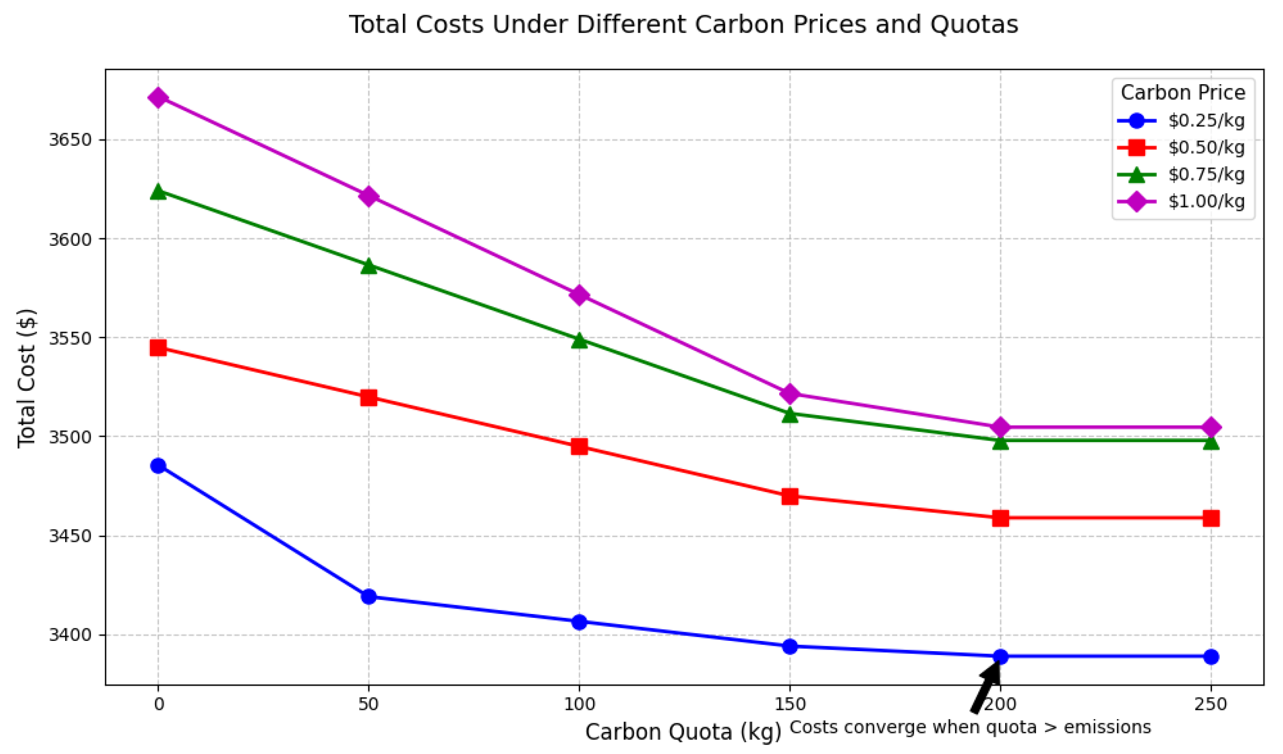
	250	167.04	−82.96	−82.96	3504.581

and Figure 11 reveal that, regarding carbon pricing and carbon quotas, these two policy levers interact to shape enterprise logistics costs. For a fixed carbon price, increasing the carbon quota directly reduces the carbon deficit (i.e., the shortfall between actual emissions and allocated allowances), thereby lowering the carbon cost. When the carbon quota is lower than actual emissions, enterprises must purchase additional allowances, leading to positive carbon costs that rise proportionally with the carbon price. For example, at a carbon price of 0.5 RMB/kg, raising the quota from 0 to 150 kg reduces carbon costs from RMB 86.08 to RMB 11.08, with a corresponding drop in total costs from RMB 3544.85 to RMB 3469.85.

Once the carbon quota exceeds actual emissions, the carbon cost becomes theoretically negative, indicating that the enterprise would hold surplus allowances that could be sold in the carbon market. In this study, negative carbon costs are treated as zero when calculating total costs; thus, beyond this threshold the total cost remains constant despite further increases in quota. This also implies that, under the given assumptions, surplus allowances provide no additional cost advantage unless explicitly monetized in practice.

From a policy perspective, an excessively low carbon price or an overly generous quota allocation both weaken the incentive for enterprises to reduce emissions. Conversely, high carbon prices combined with tight quotas can significantly raise operating costs, prompting stronger abatement actions but also risking cost burdens. Therefore, an optimal balance between carbon price and quota allocation is essential to achieving emission reduction targets while maintaining economic viability.

6. Conclusions

This study addresses the cold chain vehicle routing problem under carbon emission constraints, comparing single-mode and collaborative distribution strategies. A mixed-integer programming model is developed for the TDGVRP, incorporating carbon emissions, spatiotemporal distances, refrigeration costs, and product damage risks. Following the “cluster first, optimize later” principle, a Three-Phase Heuristic (TPH) algorithm is proposed and validated through extensive benchmark experiments.

The main findings and contributions are as follows:

• A capacity-aware spatiotemporal route construction method is proposed to generate high-quality initial truck routes, and an ALNS framework with customized destroy-and-repair operators tailored to TDGVRP characteristics significantly improves both solution quality and computational efficiency.
• The model accounts for realistic traffic conditions via time-dependent vehicle speeds, enhancing practical relevance compared to fixed-speed assumptions and improving the accuracy of urban delivery scheduling.
• Experimental results show that the joint distribution model reduces total costs by 14.4%, carbon-related costs by 23.12%, and fleet size by 25%, relative to the single-mode strategy, confirming its economic and environmental advantages in high-service-level cold chain logistics.
• Sensitivity analysis indicates that effective carbon policy requires balancing price signals with quota flexibility. Higher carbon prices (0–7 RMB/kg) achieve up to 7.12% emission reduction but raise compliance costs, with the most cost-effective abatement near 3 RMB/kg. Quota expansion under moderate pricing can cut deficits by over 80% and slightly lower total costs, while an optimal policy corridor of 1–3 RMB/kg and quotas of 120–180 kg minimizes cost growth while sustaining over 5% emission reductions.

In summary, the proposed model and algorithm offer a practical decision-support framework for sustainable cold chain logistics, delivering substantial cost savings and emission reductions under realistic operational constraints. Future extensions may incorporate stochastic demand, uncertain travel times, and dynamic carbon policies to further enhance robustness and adaptability in evolving regulatory environments.