Article

Land Use–Future Climate Coupling Mechanism Analysis of Regional Agricultural Drought Spatiotemporal Patterns

1
School of Hydraulic and Electric Power, Heilongjiang University, Harbin 150080, China
2
Heilongjiang Provincial Water Resources Research Institute, Harbin 100050, China
*
Author to whom correspondence should be addressed.
Sustainability 2025, 17(15), 7119; https://doi.org/10.3390/su17157119
Submission received: 8 July 2025 / Revised: 28 July 2025 / Accepted: 30 July 2025 / Published: 6 August 2025
(This article belongs to the Special Issue Sustainable Future of Ecohydrology: Climate Change and Land Use)

Abstract

This study assesses future agricultural drought risk in the Ganjiang River Basin under climate change and land use change. A coupled analysis framework was established using the SWAT hydrological model, the CMIP6 climate models (SSP1-2.6, SSP2-4.5, SSP5-8.5), and the PLUS land use simulation model. Key methods included the Standardized Soil Moisture Index (SSMI), travel time theory for drought event identification and duration analysis, Mann–Kendall trend test, and the Pettitt change-point test to examine soil moisture dynamics from 2027 to 2100. The results indicate that the CMIP6 ensemble performs excellently in temperature simulations, with a correlation coefficient of R2 = 0.89 and a root mean square error of RMSE = 1.2 °C, compared to the observational data. The MMM-Best model also performs well in precipitation simulations, with R2 = 0.82 and RMSE = 15.3 mm, compared to observational data. Land use changes between 2000 and 2020 showed a decrease in forestland (−3.2%), grassland (−2.8%), and construction land (−1.5%), with an increase in water (4.8%) and unused land (2.7%). Under all emission scenarios, the SSMI values fluctuate with standard deviations of 0.85 (SSP1-2.6), 1.12 (SSP2-4.5), and 1.34 (SSP5-8.5), with the strongest drought intensity observed under SSP5-8.5 (minimum SSMI = −2.8). Drought events exhibited spatial and temporal heterogeneity across scenarios, with drought-affected areas ranging from 25% (SSP1-2.6) to 45% (SSP5-8.5) of the basin. Notably, abrupt changes in soil moisture under SSP5-8.5 occurred earlier (2045–2050) due to intensified land use change, indicating strong human influence on hydrological cycles. This study integrated the CMIP6 climate projections with high-resolution human activity data to advance drought risk assessment methods. It established a framework for assessing agricultural drought risk at the regional scale that comprehensively considers climate and human influences, providing targeted guidance for the formulation of adaptive water resource and land management strategies.

1. Introduction

Against the backdrop of increasingly severe interactions between global climate change and human activities, the spatiotemporal evolution patterns of surface water cycles have undergone significant changes. Climate change has formed a composite driving mechanism by altering the thermodynamic structure of the atmosphere, reshaping the spatiotemporal distribution patterns of precipitation, and increasing the frequency and intensity of extreme hydrological and meteorological events, thereby profoundly influencing the hydrological response processes in river basins [1]. At the same time, human activities have caused systematic restructuring of the physical properties of the land cover through large-scale land use changes and water projects, which in turn have triggered secondary effects in the hydrological cycle of river basins through a “drive–response” feedback chain. The Sixth Assessment Report of the United Nations Intergovernmental Panel on Climate Change clearly states that the adverse impacts of climate change and related losses will increase in a non-linear manner with global warming. In drought-sensitive regions, this amplification effect is particularly pronounced, potentially triggering a chain reaction of systemic risks, such as the breach of water security thresholds and accelerated land degradation. Against this grim backdrop, an in-depth analysis of the mechanisms underlying agricultural drought evolution driven by multiple coupled factors has become a cutting-edge scientific issue and an urgent practical need in the field of hydrology and water resources science. Under the dual drivers of global climate change and rapid urbanization, agricultural drought has become a significant factor threatening food security and the stability of agricultural ecosystems. Agricultural drought not only directly impacts crop growth and development but leads to a sharp decline in soil organic matter content, severely weakening soil fertility and carbon storage functions, thereby forming a vicious cycle where drought stress and soil degradation reinforce each other. Therefore, accurately identifying and quantitatively assessing the relative contributions of climate change and human activities to agricultural drought, as well as their interaction mechanisms, is of great significance for revealing the formation mechanisms and evolution patterns of drought disasters. This provides an important theoretical basis for formulating scientifically sound drought risk management strategies and adaptive measures.
Therefore, establishing an agricultural drought risk assessment framework that comprehensively considers climate change scenarios and land use changes is of great scientific value and practical significance for ensuring regional food security and maintaining ecosystem stability.
Despite these recognized impacts, a critical scientific gap persists. Specifically, how to systematically predict agricultural drought risks under coupled climate–land use scenarios? Existing approaches predominantly rely on historical data analysis and real-time monitoring, lacking the integrated frameworks that combine climate model projections with land use change scenarios for forward-looking risk assessments. This limitation constrains our ability to develop proactive drought adaptation strategies, particularly in regions where climate change and rapid land use transitions create compounding risks. The central scientific challenge addressed in this study is therefore to develop and validate a predictive framework that quantifies future agricultural drought risks by systematically integrating the CMIP6 climate projections with land use scenario analysis.
Drought is described as a complex hydrological and meteorological disaster caused by a long-term imbalance between precipitation and evapotranspiration. It disrupts regional hydrological cycles, forming a cascading chain of transmission from meteorological drought to stream drought, which has serious impacts on the environment, society, and the economy [2,3]. According to the mechanism of drought occurrence, drought can be classified into five main types: meteorological drought, hydrological drought, agricultural drought, socio-economic drought, and ecological drought. There are complex interactions and transmission mechanisms between these drought types [4,5]. Agriculture, as the foundation of the national economy and an important pillar of social development, exhibits high sensitivity to drought stress in its production systems. Agricultural drought directly impacts crop growth and development and grain yield formation by significantly reducing soil moisture content, thereby threatening regional food security. As an extreme weather condition, drought disrupts agricultural production by raising temperatures and altering precipitation patterns [6,7]. From an agricultural perspective, agricultural drought specifically refers to a phenomenon in which the effective moisture content of the soil is insufficient to meet the water requirements of specific crops during their critical growth period. This water stress can lead to physiological and metabolic disorders in crops, hinder their growth and development, and ultimately result in yield losses or a decline in quality. Based on the phenological period of drought occurrence, agricultural drought can be further classified into three types: spring drought (affecting seed germination and emergence), summer drought (affecting vegetative growth and reproductive development), and autumn drought (affecting grain filling and maturation). The mechanisms by which each type affects crop yield formation exhibit significant differences [8].
Agricultural drought research encompasses three primary methodological approaches. Observational studies have utilized ground-based meteorological data to establish drought indices and historical patterns [9,10,11,12,13,14,15]. Remote sensing approaches have developed vegetation-based monitoring systems, including VCI and VHI indices, enabling real-time drought assessment [16,17,18,19]. Modeling studies have explored various simulation techniques for drought characterization and impact assessment [20,21,22,23,24,25]. Despite these advances, the existing research exhibits critical limitations in forward-looking analysis. Current methodologies predominantly focus on retrospective analysis and real-time monitoring, with insufficient integration of climate projections and land use scenarios for future risk assessment [26,27]. This methodological gap constrains our ability to predict future agricultural drought trends and to develop proactive adaptation strategies.
To gain a deeper understanding and to quantify the complex mechanisms of global climate change, the Working Group on Coupled Global Processes (WGCM) under the World Climate Research Program (WCRP) launched the Coupled Model Intercomparison Project (CMIP) two decades ago. The project has now progressed to its sixth phase (CMIP6), representing the current state-of-the-art in global climate simulation technology [28,29,30]. Although the CMIP5 and CMIP6 exhibit similar overall patterns in the spatial distribution of global climate elements, the CMIP5 still has significant uncertainties in regional-scale prediction accuracy and inter-model consistency. By contrast, the CMIP6 has significantly enhanced the reliability and stability of climate simulations by improving physical parameterization schemes, increasing model resolution, and optimizing coupling algorithms. It can also effectively reproduce the historical climate change characteristics from 1850 to 2014 and accurately reflect the combined effects of natural forcing factors (such as solar radiation changes and volcanic activity) and anthropogenic forcing factors (such as greenhouse gas emissions and aerosol emissions). Therefore, this study selects the CMIP6 climate model as the core tool for future climate scenario predictions [31,32,33,34,35]. In terms of future climate scenario settings, this study adopts three typical Shared Socio-economic Pathways (SSPs): SSP1-2.6 represents a sustainable development model under a low greenhouse gas emission background, emphasizing green transformation and prioritizing environmental protection; SSP2-4.5 reflects a moderate emission pathway under medium socio-economic development levels, embodying a balanced strategy between development and emission reduction; SSP5-8.5 corresponds to a development model with high fossil fuel dependency and high emission intensity, representing the continuation of traditional development pathways. These three scenarios cover the main possible paths of future socio-economic development, providing a scientific scenario framework for assessing the evolution of agricultural drought risks under different development models, which is helpful for formulating differentiated climate adaptation strategies [36,37].
However, the current CMIP6 models still have significant limitations in simulating key natural variability phenomena, which directly affects the accuracy of agricultural drought risk assessments. In terms of the El Niño–Southern Oscillation (ENSO) simulations, although the CMIP6 can capture the basic periodic characteristics of ENSO, it performs inadequately in quantifying the magnitude of El Niño and La Niña events’ impacts on regional water and heat conditions. More critically, existing models lack precise characterization of the intrinsic regulatory mechanisms of the climate system, making it difficult to accurately simulate the feedback effects of the ENSO disturbances and the adaptive adjustment processes of regional climate. Additionally, the short- to medium-term impacts of recent major volcanic activities (such as the 2022 Tonga submarine volcanic eruption) on the global climate system are inadequately represented within the current model framework. This is primarily due to the complex radiative forcing effects of volcanic aerosols and their nonlinear influence mechanisms on agricultural meteorological elements, which have not yet been fully incorporated into the physical processes of climate models. Based on the aforementioned modeling uncertainties, this study employs a multi-model ensemble approach to reduce systematic errors from a single model when conducting agricultural drought risk assessments by integrating the SWAT hydrological model and the PLUS land-use change model.
Hydrological models, as important scientific tools for quantitatively describing and predicting hydrological processes, play a central role in hydrological forecasting, hydrological analysis, hydraulic engineering design, and water resource planning and management [38,39]. The SWAT model (Soil and Water Assessment Tool) is an open-source distributed hydrological model developed by the Agricultural Research Service of the United States Department of Agriculture. It has become a classic tool for hydrological simulation at the watershed scale. The SWAT model adopts a physical process-based modeling approach that can quantitatively simulate the comprehensive impact of multiple environmental factors, such as land use changes, agricultural management measures, and climate change, on the hydrological cycle of a watershed at various spatial scales ranging from small watersheds to large river basins through the integration of multi-source meteorological data. The model is capable of simultaneously simulating the dynamic changes of surface water and groundwater, enabling it to not only predict the quantitative characteristics of water resources but to assess water quality conditions, thereby providing scientific support for integrated basin management [40,41,42,43].
The PLUS model (Patch-generating Land Use Simulation Model) is a cutting-edge tool for simulating land use change. It employs an integrated framework based on a dual reconstruction modeling strategy, comprising the Land Expansion Analysis Strategy (LEAS) and a cellular automaton model with multiple random patch seeds (CARS) [44,45,46,47]. Compared with traditional land use simulation models, the PLUS model has achieved significant breakthroughs in expressing spatial heterogeneity and characterizing process mechanisms. Through the LEAS module, the model can effectively identify and quantitatively analyze the driving mechanisms and their relative strengths of various land use type conversions, revealing the relative contributions of natural environmental factors and socio-economic factors to land use changes. At the same time, the CARS module uses a multi-type random patch generation algorithm, which significantly improves the model’s accuracy in simulating the spatial distribution of land use patches in complex geographical environments. The core advantage of the PLUS model lies in its ability to achieve high-precision spatial explicit simulation of land use change processes under specific scenario constraints. It not only accurately predicts changes in the number of land use types but precisely depicts the evolution characteristics of their spatial distribution patterns. This integrated modeling method provides important technical support for gaining a deeper understanding of the driving mechanisms of land use change and assessing the consequences of land use change under different development scenarios. It has significant theoretical value and practical significance for formulating scientific and reasonable land resource management strategies.
In the complex context of land use change and climate change, selecting the Ganjiang River Basin as a typical area for agricultural drought research has important scientific value and practical significance. The Ganjiang River Basin is located on the southern bank of the middle reaches of the Yangtze River. It is the most important water system and core agricultural production area in Jiangxi Province. Its unique geographical environment and climatic conditions make it an ideal place to study the mechanisms of agricultural drought evolution. In terms of geographical features, the Ganjiang River Basin has a complex and diverse topography, covering hills, mountains, plains, and other terrain types, forming significant spatial heterogeneity. The basin has a typical subtropical monsoon climate, with uneven distribution of precipitation in both time and space, large interannual variability, and frequent droughts. In particular, agricultural droughts occurring during the critical growth period of crops pose a serious threat to regional food security, water resource security, and ecosystem stability, highlighting the typicality and representativeness of the basin’s agricultural drought problem. From the perspective of human activity, with the acceleration of urbanization and industrial restructuring and upgrading in recent years, the land use pattern in the Ganjiang River Basin has undergone profound changes, mainly manifested in the significant characteristics of the continuous reduction in arable land resources and the rapid expansion of construction land. More importantly, the current agricultural, forestry, and agroforestry management models in this watershed face numerous risks and uncertainties in addressing climate change challenges. At the agricultural management level, traditional intensive farming practices heavily rely on chemical fertilizer and pesticide inputs, leading to a decline in soil organic matter and reduced water retention capacity, thereby increasing the agricultural system’s vulnerability to drought. Meanwhile, the adoption of sustainable agricultural management strategies, such as precision agriculture, water-saving irrigation, crop rotation, and fallowing, remain insufficient. In forestry management, the monoculture management model of artificial forests has reduced the hydrological regulation function and drought resilience of forest ecosystems, while multifunctional forest management strategies optimized for ecosystem service functions have not yet been widely adopted. In agroforestry composite system management, traditional crop–tree configuration patterns often lack systematic consideration of water resource efficiency and risk dispersion, and the ecological and economic benefits of integrated agroforestry management remain underutilized. These management-level challenges and differences in strategy selection directly influence the spatial distribution patterns and temporal evolution trends of regional agricultural drought risks, necessitating prioritized attention in future drought risk assessments and adaptation strategy development. Therefore, taking the Ganjiang River Basin as the research object, this study not only effectively reveals the response characteristics and evolution trends of agricultural drought under the synergistic effects of land use change and climate change, but it provides important theoretical references and decision-making support for agricultural drought monitoring and early warning risk assessment, and adaptive management in regions with similar climate and geographical conditions in southern China. This empirical study based on typical river basins has significant academic value and practical application prospects for enriching the scientific theoretical system of agricultural drought and improving regional drought risk management.
While previous studies have typically employed single models or limited model combinations to assess either land use change impacts [48] or climate change effects [49] on soil moisture separately, this study presents an innovative integrated framework that combines the PLUS, SWAT, and CMIP6 models to comprehensively investigate the synergistic effects of both land use change and climate change on soil moisture evolution and agricultural drought response. Unlike traditional approaches that focus on individual drivers, our framework enables the quantification of interactive effects between anthropogenic land use changes and natural climate variability. The PLUS model provides spatially explicit land use projections under different development scenarios, which serves as dynamic input for the SWAT hydrological model rather than using the static land use assumptions common in previous studies [50]. By combining SWAT with the PLUS-derived land use data and the CMIP6 climate projections, this study achieves the following breakthroughs compared to the existing methods: (1) it considers the coupled dynamics of the land–climate system; (2) it simultaneously considers scenario changes driven by both human and natural factors. This integrated approach offers enhanced predictive capability for soil moisture and agricultural drought changes compared to the single-model frameworks previously used in the Ganjiang River Basin [51,52].

2. Materials and Methods

2.1. Research Area Overview

The Ganjiang River, as the largest river system in Jiangxi Province, is located in the southern part of the middle and lower reaches of the Yangtze River, with geographical coordinates ranging from 113°30′ to 116°40′ east longitude and 24°29′ to 29°11′ north latitude. The Wai Zhou Hydrological Station, as the key control section where the Ganjiang River flows into Poyang Lake, is located in Wai Zhou Village, Taohua Township, Nanchang City. The station’s control basin covers an area of 80,948 km2, making it the core site reflecting the overall hydrological characteristics of the Ganjiang River Basin. The status of the watershed is shown in Figure 1. In terms of climate, the Ganjiang River Basin belongs to the subtropical humid monsoon climate zone, characterized by abundant and evenly distributed rainfall. Based on the aforementioned regional characteristics, this study selects the control area of the Wai Zhou Hydrological Station as the core research unit. By conducting high-precision soil moisture simulation analyses, the aim is to deeply reveal the intrinsic mechanisms and evolution patterns of the hydrological cycle in the Ganjiang River Basin, providing the important theoretical support and decision-making basis for scientific water resource management, ecological environment protection, and agricultural drought risk prevention and control in the basin.

2.2. Data Source: Preprocessing

This study is based on land use dynamics monitoring data from 2000 to 2020. A time series analysis framework was constructed with a 10-year interval, and the land use classification system includes major types, such as farmland, forestland, grassland, water area, and construction land. Fourteen land use drivers (X1–X14) were categorized into three groups and used as model input variables: natural factors, which include terrain factors (elevation, slope), climate factors (annual average precipitation, annual average temperature), and environmental factors (soil type, distance to water bodies). A Digital Elevation Model (DEM) data is sourced from the Geospatial Data Cloud (http://www.gscloud.cn, accessed on 1 July 2025) and utilizes the ASTER Global Digital Elevation Model Version 3. Socio-economic factors comprise GDP, population density, and distance to roads, which reflect human activity intensity and accessibility conditions. Technology-type factors include the nighttime light index, which serves as a proxy for technological development and urbanization levels. All driver data have been standardized and calculated using Euclidean distances to ensure the data quality and consistency of model inputs. To meet the model calculation accuracy requirements, all raster data were uniformly resampled to a spatial resolution of 30 m and spatially registered using the WGS-1984-UTM-ZONE-50N projection coordinate system. The detailed sources, processing methods, and technical parameters of various data categorized by factor types are shown in Table 1.
The meteorological data are sourced from the Climate Simulation Center of the National Aeronautics and Space Administration (NASA) (https://www.nccs.nasa.gov, accessed on 1 July 2025). In this study, 14 global climate models were selected from the CMIP6 multi-model ensemble as climate forcing data sources. This study selected three typical shared socio-economic pathway scenarios: SSP1-2.6 (low emissions scenario), SSP2-4.5 (medium emissions scenario), and SSP5-8.5 (high emissions scenario). The time series covers the baseline period (1970–2014) and the future projection period (2025–2100). These three scenarios are widely representative in climate change research and reflect different possible future pathways for greenhouse gas emissions and socio-economic development. Given that global climate models (GCMs) have relatively coarse spatial resolution and cannot meet the accuracy requirements for regional-scale hydrological simulation, this study employs statistical downscaling techniques to convert the coarse-resolution climate information from GCMs into fine-scale spatial data suitable for watershed-scale analysis. To ensure data quality and consistency, all CMIP6 climate data have undergone systematic bias correction and spatial downscaling, resulting in a high-quality climate driver dataset with a temporal resolution of daily data and a spatial resolution of 0.25° × 0.25°, as shown in Table 2.

2.3. Research Framework

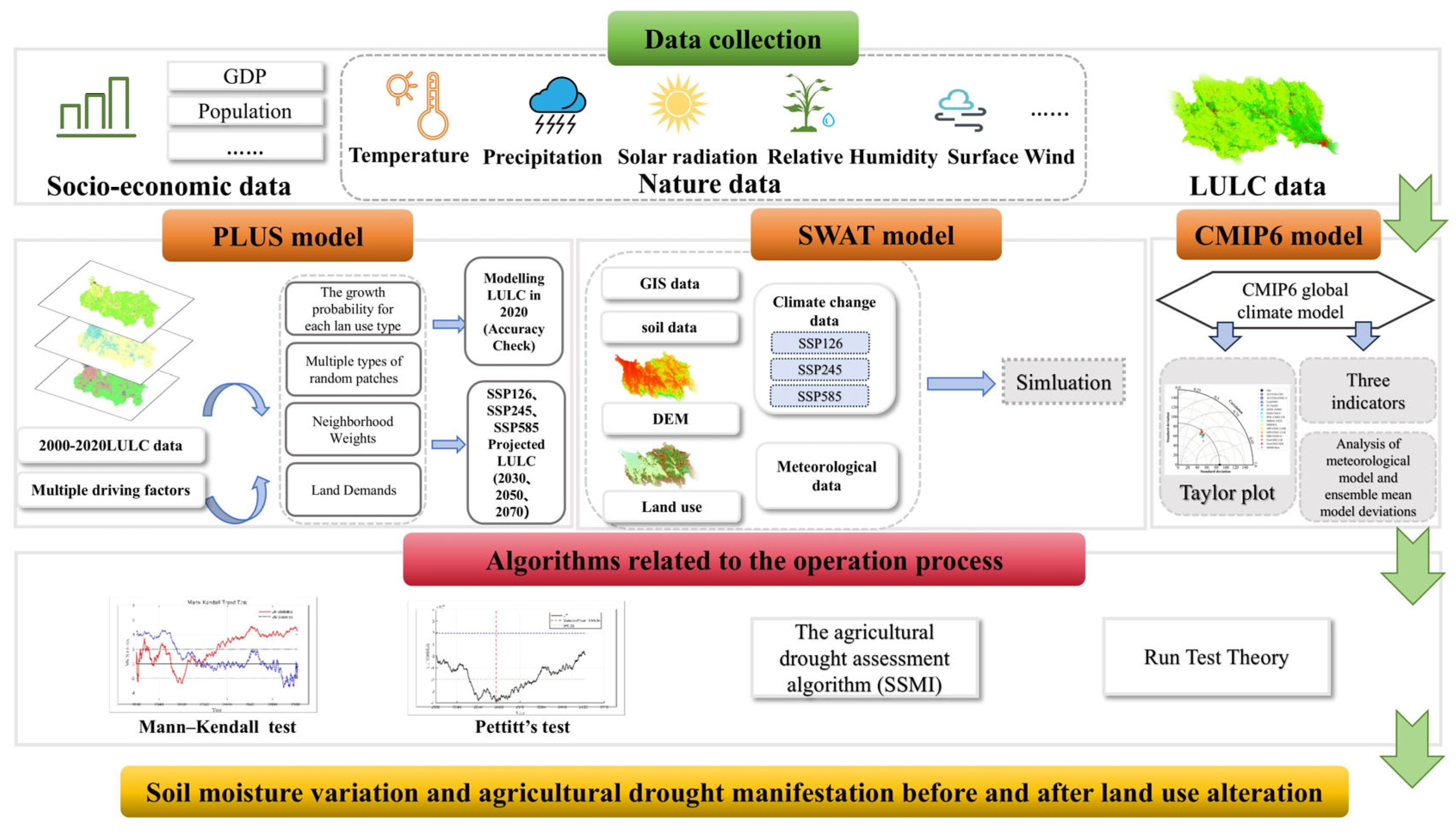
This study established a coupled response analysis framework for land use change, soil moisture, and agricultural drought in the Ganjiang River Basin, aiming to systematically elucidate the driving mechanisms of land use change on soil moisture dynamics and agricultural drought evolution. The research methodology follows a systematic analysis process of “data acquisition–model coupling–algorithm integration–result output”, ensuring the scientific rigor of the research methods and the reliability of the results. This study established a multi-source heterogeneous data integration system encompassing socio-economic factors, natural environmental factors, and land use and land cover (LULC) changes, providing comprehensive data support for the analysis of complex driving mechanisms. In terms of methodological construction, this study integrated the PLUS–SWAT–CMIP6 multi-model coupling framework with diverse statistical algorithms, such as the Mann–Kendall trend test, the Pettitt inflection point test, the standardized soil moisture index, and travel time theory, forming a comprehensive methodological framework comprising “process simulation–statistical analysis–risk assessment”. This integrated research framework demonstrates significant theoretical innovation and methodological advantages. From a theoretical perspective, the quantitative separation of the effects of land use change and climate change on agricultural drought through multi-model coupling has enriched our scientific understanding of human–land system interactions. From a methodological perspective, the technical system constructed can effectively handle complex multi-scale, multi-factor coupling relationships, providing a systematic solution for regional agricultural drought risk assessment. The methodological framework established in this study not only provides technical support for the scientific management of water resources and agricultural drought prevention and control in the Ganjiang River Basin, but it provides important theoretical references and technical guidance for water resource management, optimal land use allocation, and the construction of agricultural drought monitoring and early warning systems in similar river basins in the southern monsoon climate zone of China. It has broad application value. The framework of this study is illustrated in Figure 2.

2.4. SWAT Model Calibration and Validation

The SWAT model simulates complex hydrological processes by dividing the study area into multiple sub-basins, which are further subdivided into hydrological response units (HRUs) with similar land use, soil type, and topographical characteristics [53]. The core mechanism of this model is based on the water balance principle of individual landscape units, which accurately simulates the water cycle of a watershed through hydrological driving processes [54]. To ensure the reliability of model parameters and to optimize simulation accuracy, this study used the SWAT-CUP (SWAT Calibration and Uncertainty Procedure) to systematically calibrate and validate the model.
Prior to calibration, a comprehensive parameter sensitivity analysis was conducted using the SUFI-2 (Sequential Uncertainty Fitting version 2) algorithm embedded in SWAT-CUP. The sensitivity analysis employed the multiple regression method to calculate t-statistics and p-values for each parameter, where parameters with higher absolute t-values and lower p-values (p < 0.05) were identified as more sensitive parameters [55]. A total of 25 key hydrological parameters related to surface runoff, groundwater flow, evapotranspiration, and channel routing were initially selected for sensitivity analysis, and the top 15 most sensitive parameters were subsequently retained for model calibration based on their ranking.
Following standard model evaluation protocols, the observed data is split in a 2:1 ratio, with 2/3 of the data used for model calibration and 1/3 used for independent validation. Based on data availability and model stability, the training period was determined to be 1993–2004, and the validation period was determined to be 2005–2014 [56]. Model performance evaluation employs a widely recognized statistical indicator system, including the coefficient of determination (R2) to quantify the linear correlation between simulated values and observed values, the Nash–Sutcliffe efficiency coefficient (NSE) to assess the model’s overall predictive capability, the percentage bias (PBIAS) to reflect the model’s systematic bias, and the root mean square error ratio (RSR) as a standardized root mean square error indicator, to comprehensively evaluate the model’s goodness of fit. This multi-indicator assessment framework can comprehensively quantify the simulation performance of the model under different hydrological conditions, providing a reliable scientific basis for subsequent hydrological analysis and prediction.
R 2 = i = 1 n ( Q m , i Q m , a v g ) ( Q p , j Q p , a v g ) 2 i = 1 n ( Q m , i Q m , a v g ) 2 i = 1 n ( Q p , i Q p , a v g ) 2
N S E = 1 i = 1 N Q m , i Q p , i 2 i = 1 N Q m , i Q m , a v g 2
P B I A S = i = 1 N ( Q p , i Q m , i ) i = 1 N Q m , i × 100 %
R S R = i = 1 N ( Q m , i Q p , i ) 2 i = 1 N ( Q m , i Q m , a v g ) 2
where Q m , i is the measured flow rate in m3/s, Q m ,   avg   is the long-term measured average flow rate in m3/s, Q p , i is the simulated flow rate in m3/s, Q p ,   avg   is the long-term simulated average flow rate in m3/s, and N is the length of the measured time series. The Nash–Sutcliffe Efficiency Coefficient (NSE) serves as the core evaluation metric in Equation (2). The closer the NSE value is to 1, the higher the agreement between the model simulation results and the measured data, indicating better model performance. When NSE = 1, it indicates that the simulated values are completely consistent with the observed values; when NSE = 0, it indicates that the model’s predictive ability is equivalent to using the observed mean as the predicted value; when NSE < 0, it indicates that the model’s performance is inferior to simple mean prediction. The coefficient of determination R2 is shown in Equation (1), and is used to quantify the strength of the linear correlation between the model output and the observed data. The R2 value ranges from 0 to 1, with higher values indicating that the model better explains the variability in the observed data. According to the evaluation criteria in the field of international hydrological modeling, when NSE ≥ 0.5 and R2 ≥ 0.6, the model’s fitting accuracy is considered to have reached an acceptable level and can meet the basic requirements for hydrological process simulation. This evaluation standard provides objective criteria for the quantitative assessment of model performance, ensuring the scientific nature and reliability of research results.

2.5. PLUS Model

Based on the complex driving mechanisms of land use change, this study constructed a comprehensive driving factor system that includes natural and human factors. Select 10 key driving factors, including elevation, gross domestic product (GDP), population density, nighttime light index, slope, annual average precipitation, annual average temperature, soil type, distance to water bodies, and road distance. Through an in-depth analysis of the spatiotemporal evolution characteristics of land use in the study area, a combination of expert knowledge and statistical analysis was employed to dynamically adjust and to optimize the weight parameters of each driving factor, thereby accurately reflecting the contribution of different factors to land use changes.
Model accuracy is verified using the Kappa consistency coefficient for quantitative assessment. The Kappa coefficient is an important statistical indicator for measuring the degree of consistency between classification results and actual conditions. It can effectively eliminate the influence of random classification, and its value ranges from 0 to 1. According to internationally recognized accuracy evaluation standards, when the Kappa coefficient is greater than 0.75, it indicates that the classification accuracy of the model has reached a good level and can reliably reflect the spatial variation characteristics of landscape patterns. The Kappa coefficient is particularly suitable for a comparative analysis of multi-phase remote sensing images, providing an objective quantitative basis for assessing the accuracy of land use change simulations. The calculation formula is as follows:
  Kappa   = P o P c P p P c
where P o represents the simulated correct grid ratio, P c represents the simulated correct ratio under random conditions, and P p represents the simulated correct ratio under ideal conditions. The basic parameters for simulating the future spatial distribution of land use under specific conditions include domain weights and cost matrices, and the results of weight calculations may also cause changes in accuracy.
W i = Δ TA i Δ TA min Δ TA max Δ TA min
where W i represents the neighborhood weight coefficient of land use type i, Δ T A i represents the area change of land type i during the study period, Δ T A max represents the maximum area change during the study period, and Δ T A min represents the minimum area changes during the study period, respectively.
Under the theory of optimizing land use space allocation in the Ganjiang River Basin, the transfer cost matrix should be designed differently based on policy directions and spatial constraints under different development scenarios. This study is based on multi-source data fusion and scenario analysis theory, comprehensively considering key factors, such as ecological protection policies, economic development needs, urbanization processes, and the ecological and economic costs of land use conversion. A scenario-specific transfer cost matrix parameter system was constructed. Through a systematic analysis of the natural geographical conditions, socio-economic development levels, and land use policy constraints of the study area, a domain weighting allocation mechanism was established based on a combination of expert knowledge and field research. Based on the specific needs of different development scenarios, corresponding conversion cost parameters between land use types were set, forming a differentiated transfer cost matrix under multiple scenarios (see Table 3 for details).

2.6. CMIP6 Climate Model

The Taylor plot serves as a standardized diagnostic tool for multi-mode ensemble assessment, enabling the comprehensive display of differences between model simulation performance and observational benchmarks within a unified two-dimensional space. This method uses geometric transformations in the polar coordinate system to organically integrate the three core statistical indicators in model evaluation—correlation coefficient (r), root mean square error (RMSE), and standard deviation ratio (SD)—to achieve the visualization and integration of multidimensional statistical information. In the context of the CMIP6 multi-model comparison project, Taylor plots can quickly identify performance differences between models, providing objective quantitative evidence for selecting high-performance climate models.
RMSE = x i y i 2 1 n i = 1 n x i y i 2
R = i = 1 n x i x ¯ y i y ¯ i = 1 n x i x ¯ 2 y i y ¯ 2
S T D = 1 n i = 1 n X i X ¯ 2
where x i is the observed value for each month, y i is the simulated value for each model for each month, x ¯ is the average value of the monthly observed data, y ¯ is the average value of the monthly simulated data, and n is the number of monthly simulated values.

2.7. Agricultural Drought SSMI

The Standardized Soil Moisture Index (SSMI) is a quantitative agricultural drought assessment indicator based on an historical soil moisture time series, which can effectively characterize the spatiotemporal evolution of agricultural drought at regional scales. This index is calculated by statistically standardizing long-term soil moisture observation data, eliminating seasonal fluctuations and interannual trends in the time series, thereby objectively reflecting the deviation of soil moisture conditions relative to historical averages. The SSMI is constructed based on probability distribution theory, which converts raw soil moisture data into standardized dimensionless indices, enabling the assessment of drought conditions across different temporal and spatial scales. When the SSMI value is significantly lower than the historical statistical threshold, it indicates that the soil moisture deficit exceeds the normal fluctuation range, posing a potential risk of agricultural drought. This standardized processing method effectively overcomes the limitations of absolute soil moisture values in different geographical environments and provides a unified evaluation standard for regional drought monitoring.
This study uses soil moisture products from the TerraClimate high-resolution climate dataset as the primary data source. This dataset has the advantages of strong temporal and spatial continuity and high accuracy, which can meet the needs of precise monitoring of agricultural drought at the regional scale. By calculating the SSMI time series on a monthly basis over many years, a long-term monitoring system for agricultural drought in the study area was established, providing a reliable scientific basis for the agricultural drought risk assessment and early warning.
S S M I i , j = S M i , j S M j ¯ j
where i represents the observation year from 1990 to 2018, j denotes the observation month from January to December, and SMJ and ∂j are the average and standard deviation of soil moisture for month j, respectively. The SSMI is dimensionless and is used to detect drought. When the SSMI is greater than 0, it can be considered wetter than the multi-year average for the same period; otherwise, it is drier.
The SSMI drought classification thresholds follow the standardized framework established by McKee et al. (1993) for drought indices, which has been successfully adapted for soil moisture applications by Xu et al. (2021) and further validated in agricultural drought studies by Krueger et al. (2019), Modanesi et al. (2020), and Tramblay and Quintana Seguí (2022) [57,58,59,60,61]. These thresholds are based on standard normal distribution percentiles and have been extensively validated in global soil moisture drought monitoring (Dorigo et al., 2013) [62]. The SSMI value can be classified into five levels based on different types. When −0.5 < SSMI, it indicates a non-drought state, meaning that soil moisture is normal and there are no signs of drought. When −1 < SSMI ≤ −0.5, it indicates a mild drought state, meaning that soil moisture is slightly insufficient but has not yet caused serious harm to the ecology and agriculture. When −1.5 < SSMI ≤ −1, the region is classified as moderately dry, with a noticeable shortage of soil moisture that can cause damage to water-sensitive crops and ecosystems. When −2 < SSMI ≤ −1.5, the drought is classified as severe, with severe soil moisture deficiency, causing significant harm to ecosystems and agriculture. When SSMI ≤ −2, the drought is classified as extreme, representing the most severe drought condition, which can lead to widespread crop failure and can cause severe damage to the ecological environment. The specific drought classification criteria are shown in Table 4.

2.8. Runs Theory

As a classic method of time series analysis, run theory defines segments of time series that continuously satisfy specific conditions as a run unit, providing a rigorous mathematical framework for the objective identification and quantitative characterization of drought events. In agricultural drought analysis, when the Standardized Soil Moisture Index (SSMI) is continuously below or equal to the preset drought threshold, the time period constitutes a complete drought cycle, thereby enabling precise definition of the temporal boundaries of drought events [63,64,65,66]. The drought identification algorithm based on the travel time theory systematically extracts the key time attributes of each drought travel time, including basic parameters such as start time, end time, and duration, through gradual scanning of the SSMI time series. Based on this, a drought intensity classification system is established by combining the distribution characteristics of the SSMI values to enable the accurate classification of drought events of different levels. Through statistical analysis of the identified drought processes, key statistical parameters such as the occurrence frequency, average duration, maximum duration, and peak intensity of the drought events can be quantitatively calculated [67,68,69].

3. Results

3.1. SWAT Model Parameter Calibration and Validation

The SWAT hydrological model constructed in this study is based on long-term observational data from 1990 to 2014 at hydrological stations in the Ganjiang River Basin on the south bank of the middle and lower reaches of the Yangtze River, including multi-source hydrological data, such as soil moisture, meteorological elements, and surface runoff. A two-year warm-up period is set during model operation to ensure that model state variables are fully initialized and to eliminate the potential impact of initial conditions on the simulation results. Subsequently, the SWAT-CUP integrated platform was used to conduct systematic sensitivity analysis, uncertainty quantification, parameter calibration, and model validation on the model, thereby establishing a comprehensive model evaluation system.
In order to accurately identify the key parameters affecting the simulation of hydrological processes in river basins, this study conducted a comprehensive parameter sensitivity analysis based on the multi-algorithm integration framework of the SWAT-CUP software(version 5.3, 2W2E GmbH, Zurich, Switzerland) platform. This platform integrates a variety of advanced sensitivity analysis algorithms, which can systematically quantify the contribution of individual parameter changes to the model output response, providing a scientific basis for parameter optimization. By conducting sensitivity tests on each physical parameter involved in the watershed hydrological model, we finally selected 21 key parameters that have a significant impact on soil moisture simulation and ranked them scientifically according to their sensitivity.
The results of the sensitivity analysis, as shown in Table 5, indicate that five parameters—Deep Aquifer Percolation Fraction, SCS Curve Number, Slope Length for Lateral Subsurface Flow, Shallow-Aquifer Return Flow Threshold, and Main Channel Width—exhibit the highest sensitivity characteristics within the model parameter system. These parameters have a decisive influence on the simulation accuracy of the spatiotemporal distribution of soil moisture in the watershed. Their numerical changes can significantly alter the hydrological response characteristics of the model. Therefore, they require special attention and precise calibration during the model calibration process.
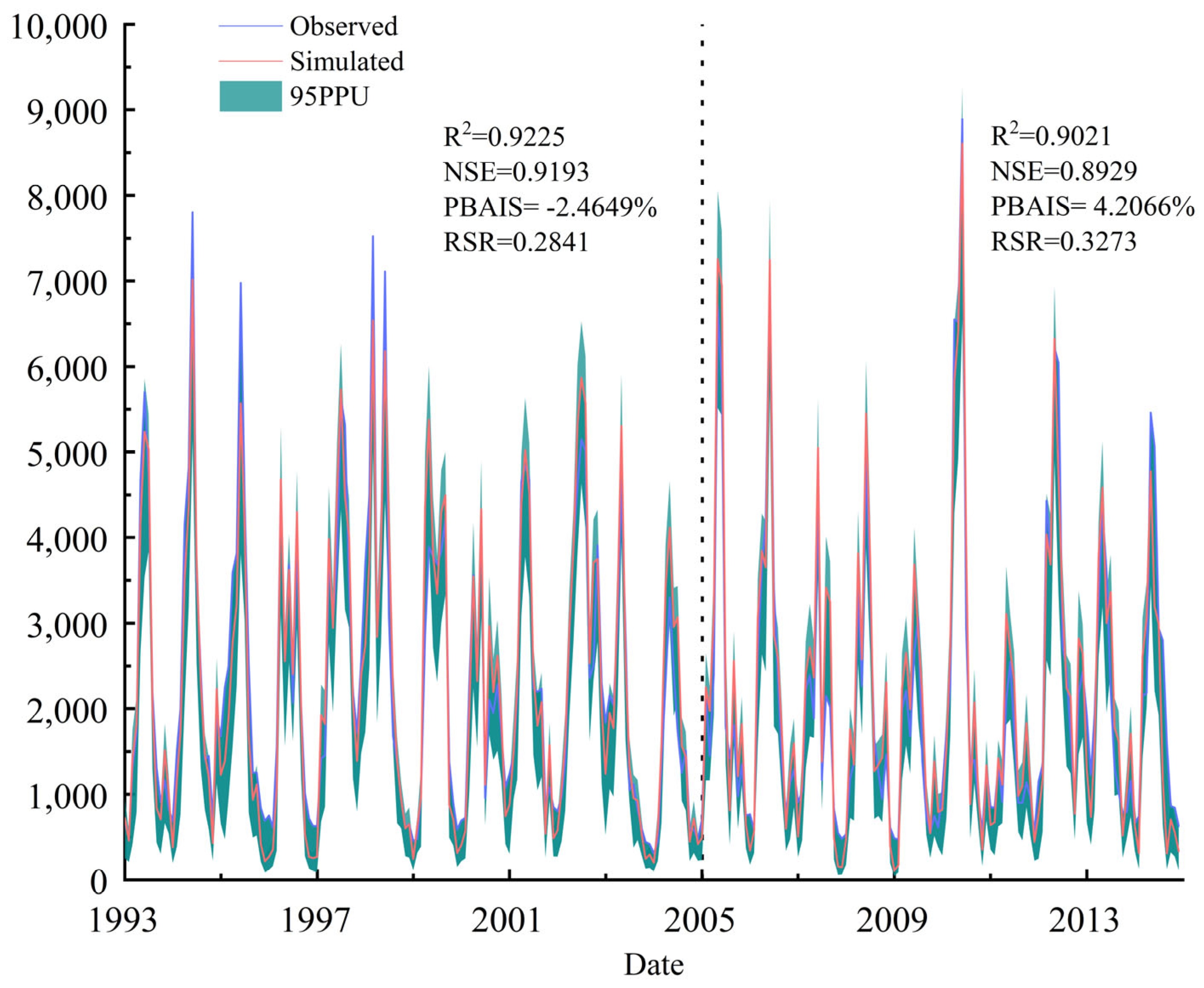
Based on long-term hydrological data from the Ganjiang River Basin’s external hydrological stations from 1970 to 2014, this study employed the SWAT distributed hydrological model to establish a two-stage model evaluation system for the calibration period (1993–2004) and validation period (2005–2014) (Figure 3). The results of the time series analysis show that, during the period from 1993 to 2014, the monthly runoff in the Ganjiang River Basin exhibited significant spatiotemporal variability. The annual runoff process displayed a complex fluctuation pattern characterized by multiple peaks and valleys, reflecting the comprehensive regulation of the basin’s hydrological processes by multiple factors, such as precipitation, evapotranspiration, and groundwater recharge. This pattern exhibited distinct seasonal periodic changes and interannual variability. To comprehensively assess the uncertainty characteristics of model predictions, this study employed the SUFI-2 optimization algorithm integrated into the SWAT-CUP platform to construct a 95% prediction uncertainty band (95PPU). By calculating the statistical boundaries of L95PPU (2.5th percentile) and U95PPU (97.5th percentile), this study quantitatively assessed the uncertainty distribution range of monthly runoff simulations in the Ganjiang River Basin from 1993 to 2014.
The results of the model performance evaluation indicate that all statistical indicators meet the international standards for hydrological modeling. The coefficient of determination (R2) values for both the calibration period and the validation period exceeded the threshold of 0.75, reaching 0.9225 and 0.9021, respectively, indicating a high degree of linear correlation between the simulated runoff and the measured runoff. The Nash–Sutcliffe efficiency coefficient (NSE) was 0.9193 and 0.8929 during the calibration and validation periods, respectively, both exceeding the excellent standard of 0.97. The closer the NSE value is to 1, the better the overall predictive performance of the model. The percentage bias (PBIAS) during the calibration period was −2.4649%, and during the validation period it was 4.2066%, with absolute values both within the acceptable range of ±10%, indicating that the model exhibits no significant systematic bias in long-term water balance. The standardized root mean square error (RSR) was 0.2841 during the calibration period and 0.3273 during the validation period, both below the excellent standard of 0.5, further validating the model’s high-precision simulation capability.
The assessment results based on multiple statistical indicators demonstrate that the SWAT hydrological model constructed achieves an acceptable level of performance in the Ganjiang River Basin. The model can reasonably characterize the hydrological process characteristics of the basin, providing a useful modeling tool for subsequent hydrological situation analysis, water resource assessment, and climate change impact studies. However, potential sources of uncertainty should be acknowledged, including climate model bias in meteorological forcing data, spatial resolution mismatches between different input datasets, and inherent limitations in model parameterization that may affect simulation accuracy.

3.2. CMIP6 Global Climate Model Analysis

3.2.1. Comparison of Taylor Diagrams Between Meteorological Models and Ensemble Average Models

This study is based on long-term observational data from 15 hydrological stations in the Ganjiang River Basin on the southern bank of the middle and lower reaches of the Yangtze River from 1970 to 2014. A multi-indicator integrated assessment system was employed to systematically evaluate the regional simulation performance of the 15 CMIP6 global climate models. The evaluation indicator system includes multi-dimensional statistical diagnostic tools, such as relative deviation, correlation coefficient, root mean square error, relative error, and Taylor plots. Through quantitative analysis of the consistency between the simulation results of each climate model and the observed reference, the optimal model combination is identified, and an ensemble prediction system is constructed. In the Taylor plot (Figure 4), both the horizontal and vertical axes represent normalized standard deviation values, which are used to quantify the variability characteristics of the CMIP6 model simulations relative to the observed data. The curved contour lines represent the distribution of correlation coefficients, reflecting the strength of the linear relationship between the model outputs and the observed data. The closer the contour line values are to 1, the more consistent the temporal variation patterns between the two are. By analyzing the spatial distribution characteristics of the Taylor plot, one can intuitively identify climate models with outstanding simulation performance and select the optimal set of five models for ensemble averaging.
This multi-model comparative analysis framework not only objectively evaluates the applicability of individual climate models at the regional scale, as shown in Figure 4, but it provides a scientific basis for constructing a high-precision multi-model ensemble prediction system, thereby laying a reliable model foundation for future climate change scenario analysis and impact assessment in the Ganjiang River Basin.
In the field of temperature prediction, this study conducted a systematic multi-model comparison analysis of temperature predictions under future climate change scenarios for the Ganjiang River Basin. The assessment results indicate that all 15 CMIP6 climate models included in the analysis demonstrated excellent performance in regional temperature simulation. The correlation coefficients of all models exceeded the high threshold of 0.97, indicating a strong linear correlation between the model outputs and the observed temperature data, and the ability to accurately capture the temporal evolution characteristics of temperature changes. The model accuracy assessment shows that the root mean square error (RMSE) of all 15 climate models is within 2.98, indicating that the systematic deviation between the model predictions and the observed values is extremely small, and the simulation accuracy has reached the excellent standards in the field of climate modeling. Further statistical analysis indicates that the models also exhibit good consistency in simulating extreme temperatures: the standard deviation range for daily maximum temperature (tasmax) is 7.83–7.98, and the standard deviation range for daily minimum temperature (tasmin) is 7.64–7.79, with small coefficients of variation between the models. The above statistical characteristics indicate that, despite the differences in physical parameterization schemes and numerical algorithms among the different CMIP6 models, they exhibit high consistency and reliability in simulating temperature elements in the Ganjiang River Basin. This result provides a solid scientific basis for subsequent climate change prediction and impact assessment based on multi-model ensembles, ensuring the credibility and accuracy of regional climate change research.
In the field of precipitation forecasting, this study conducted a comprehensive evaluation of the precipitation forecasting capabilities of the 15 CMIP6 climate models in the Ganjiang River Basin. A preliminary analysis indicates that all evaluated models possess a certain level of precipitation simulation capability. However, through a detailed analysis using multi-dimensional statistical indicators, significant performance differences were identified among the models. Based on multiple evaluation criteria, including correlation analysis, error statistics, and Taylor plots, four outstanding models were identified for precipitation simulation: ACCESS-ESM1-5, EC-Earth3, INM-CM4-8, and MPI-ESM1-2-HR. These four preferred models demonstrate significant advantages in capturing the spatiotemporal variability of precipitation, reproducing the accuracy of extreme precipitation events, and simulating seasonal precipitation cycles. Based on the results of the optimal model selection, this study adopted an equal-weight ensemble averaging method to construct a multi-model ensemble prediction system (Multi-Model Mean-Best, MMM-Best), which further improved the overall accuracy of precipitation prediction through the complementary nature and uncertainty cancellation effects between models. The validation results of the MMM-Best ensemble model demonstrate significant performance improvements in precipitation simulation. The correlation coefficient between the ensemble model and the observed data reached 0.72, with the root mean square error controlled within 60.74 mm. This level of accuracy significantly outperforms the performance of a single model, indicating that the multi-model ensemble method can effectively reduce the systematic biases of individual models and enhance the reliability of precipitation forecasts. The optimized model combination provides high-precision climate-driven data for future precipitation change scenario analysis and hydrological impact assessment in the Ganjiang River Basin.
Based on the aforementioned multi-model performance evaluation results, this study selected the MMM-Best ensemble model as the optimal driving model for regional climate change prediction, which will be used to simulate the temperature and precipitation changes in the Ganjiang River Basin under different emission scenarios from 2025 to 2100. The study sets the period from 1970 to 2014 as the historical baseline period and the period from 2025 to 2100 as the future climate change prediction period. By constructing a long-term climate change scenario analysis framework, this study systematically reveals the spatiotemporal evolution patterns of hydrological and meteorological elements in the Ganjiang River Basin. Compared with previous studies based on single climate models or simplified scenario settings, the multi-model ensemble prediction method used in this study can more comprehensively characterize the complexity and uncertainty of future climate change. By comparing and analyzing the differences in climate responses under different shared socio-economic pathways (SSPs), this study has explored in depth the mechanisms by which the intensity of human activities affects regional climate systems, providing a more reliable scientific basis for accurately grasping the future hydrological and meteorological evolution trends in the Ganjiang River Basin. In the predictive analysis process, this study fully considered various sources of uncertainty in future climate scenarios, including differences in greenhouse gas emission pathways, diversity in socio-economic development models, and the impact of intrinsic variability in the climate system. This multi-scenario integration analysis framework not only quantifies the possible range of future climate change but provides scientific uncertainty information for regional climate risk assessment and adaptation strategy formulation, significantly enhancing the scientific rigor and practicality of climate change impact research.

3.2.2. Future Climate Change Scenarios

Based on three shared socio-economic pathways (SSP1-2.6, SSP2-4.5, and SSP5-8,5), this study conducted a systematic predictive analysis of precipitation changes in the Ganjiang River Basin during different future periods (Table 6). The analysis of precipitation changes in the near-term prediction period (2030–2040) indicates that all three emission scenarios exhibit a mild humidification trend. Under the SSP1-2.6 scenario, the predicted precipitation is 1607.81 mm, representing a 5.13% increase compared to the baseline period. Under the SSP2-4.5 scenario, the predicted precipitation is 1552.93 mm, representing a 1.54% increase. Under the SSP5-8.5 scenario, the predicted precipitation is 1587.83 mm, with an increase of 3.82%. The average predicted precipitation across the three scenarios is 1582.86 mm, with an average increase of 3.50%, indicating that precipitation in the Ganjiang River Basin shows an overall upward trend, but the increase is relatively moderate, reflecting the gradual nature of short-term changes in the climate system. The precipitation changes during the mid-term forecast period (2041–2060) exhibit significant scenario differentiation characteristics. Under the SSP1-2.6 scenario, the predicted precipitation decreases sharply to 3253.63 mm, with a relative change rate as high as 112.74%. This substantial precipitation increase results from coupled climate mechanisms inherent to the SSP1-2.6 pathway and regional physiographic characteristics. Rapid decarbonization under SSP1-2.6 induces nonlinear perturbations in East Asian monsoon circulation, enhancing moisture flux within the subtropical precipitation belt. The basin’s subtropical–temperate transitional position increases sensitivity to circulation anomalies, notably Western Pacific subtropical high shifts and South China Sea monsoon intensification, which strengthen Pacific moisture advection. Orographic enhancement occurs through the region’s elevation gradient, where topographic forcing intensifies moisture convergence and convective development. The SSP1-2.6 aerosol reduction trajectory simultaneously modifies cloud microphysics, increasing precipitation efficiency and convective intensity across this topographically heterogeneous region.
This exceptionally significant increase may be attributed to the complex climate feedback mechanisms triggered by stringent carbon emission reduction policies under this scenario, including adjustments in atmospheric composition structure, changes in air–sea interaction patterns, and nonlinear responses in regional water cycle processes. By contrast, the rates of change under the SSP2-4.5 and SSP5-8.5 scenarios were relatively moderate, at 6.37% and 8.20%, respectively, highlighting the significant differences in the impact of different emission pathways on regional precipitation systems. The precipitation forecast values under the SSP1-2.6, SSP2-4.5, and SSP5-8.5 scenarios are 1685.43 mm, 1651.00 mm, and 1692.89 mm, respectively, with corresponding change rates of 10.21%, 7.95%, and 10.69%. The average predicted precipitation for the three scenarios is 1676.44 mm, with an average increase of 9.62%. Compared to the significant fluctuations in the medium-term period, the long-term prediction period exhibits a relatively stable trend of increased precipitation. This change indicates that, after a period of adjustment in the climate system during the mid-term, the precipitation pattern in the Ganjiang River Basin gradually stabilizes, providing a relatively stable climate background for long-term water resource planning and management.
The Ganjiang River Basin is located in a subtropical monsoon climate zone. The continuous rise in temperature will significantly intensify regional evapotranspiration intensity, leading to a restructuring of the spatiotemporal distribution pattern of precipitation, posing a severe challenge to agricultural irrigation systems. This study analyzed the predicted values and change rates of annual average temperatures in the Ganjiang River Basin under three emission scenarios (SSP1-2.6, SSP2-4.5, and SSP5-8.5) (Table 7). The analysis of temperature changes during the near-term forecast period (2030–2040) shows that the warming magnitudes under the three scenarios are relatively similar, but differences in emission intensity have begun to emerge. Under the SSP5-8.5 high-emission scenario, the temperature increase is the most significant, reaching 12.87%, reflecting the strong disruptive effects of rapidly rising greenhouse gas concentrations on the short-term climate system. The temperature increases under the SSP1-2.6 and SSP2-4.5 scenarios are relatively moderate and similar in magnitude, indicating that the climate effects of different emission reduction policies have not yet fully manifested themselves in the near term. Compared with the average temperature of 18.35 °C during the baseline period, the average temperature increase during the near-term forecast period is 11.96%, indicating that the Ganjiang River Basin enters a significant phase of climate warming. The mid-term forecast period (2041–2060) exhibits distinct scenario differentiation characteristics. Under the SSP5-8.5 scenario, the predicted temperature reaches 21.43 °C, with the warming effect significantly exceeding that of the SSP1-2.6 and SSP2-4.5 scenarios, highlighting the cumulative warming effect of high-emission pathways. The average temperature forecast for the three scenarios is 21.1 °C, an increase of 0.55 °C compared to the near-term forecast period, indicating that the warming trend of the climate system is accelerating further in the mid-term. Temperature changes in the long-term forecast period (2061–2100) show significant path dependency. Under the SSP1-2.6 scenario, the warming rate tends to stabilize, validating the effectiveness of strict carbon emission reduction policies in long-term climate mitigation. However, under the SSP5-8.5 scenario, the predicted temperature rises to 23.15 °C, with the temperature difference between the SSP5-8.5 and SSP2-4.5 scenarios widening to 1.49 °C. This significant temperature divergence poses a serious threat to the stability of the global climate system. Long-term high temperatures may trigger frequent extreme droughts and heavy precipitation events, exerting major impacts on regional hydrological processes and agricultural production safety. It is imperative to formulate corresponding climate adaptation strategies.

3.3. Land Use Change

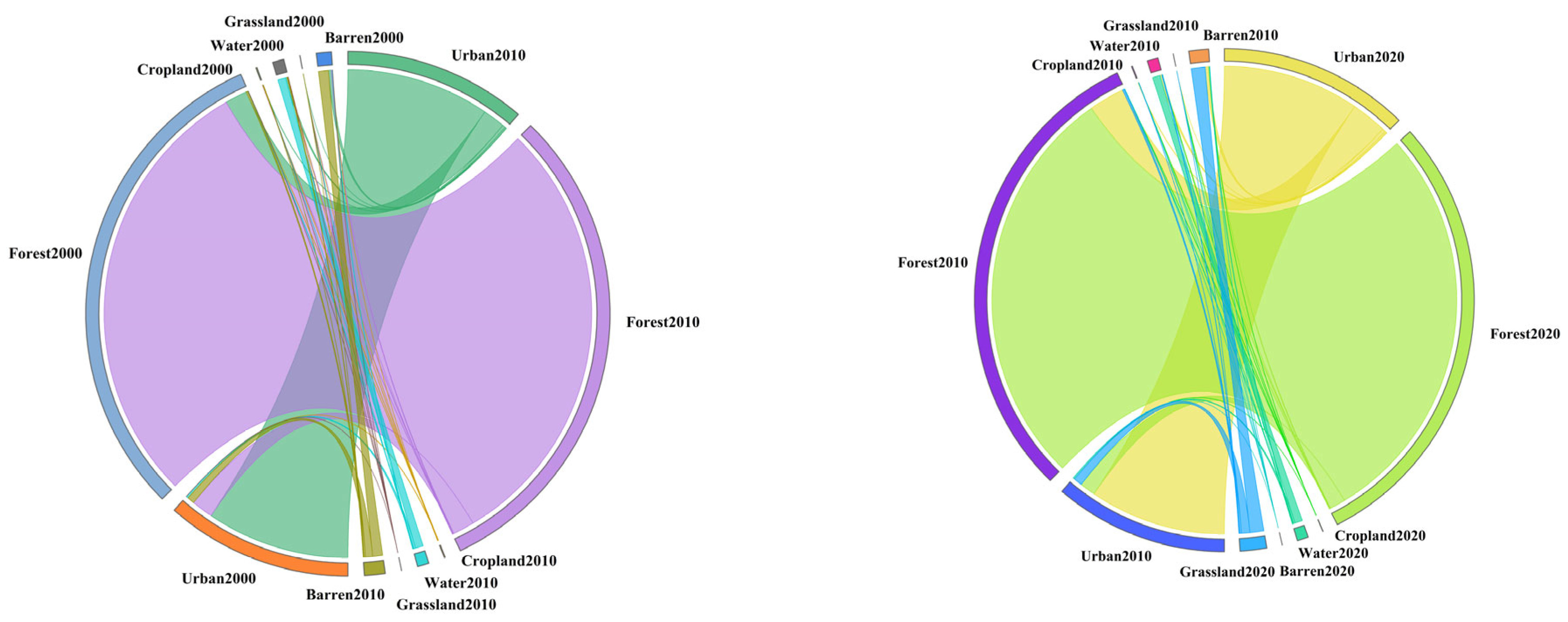
The Chord Diagram is a specialized visualization tool designed to represent the dynamic transformation relationships between land use types. It employs a circular layout to intuitively present the information contained in a multidimensional transition matrix. In this graphical system, each land use type (including farmland, forestland, construction land, water bodies, etc.) is distributed as arc segments along the circumference of a circle. The length of each arc segment is proportional to the area proportion of the corresponding land use type, thereby reflecting the spatial distribution characteristics of different land use types within the study area [70,71]. The mutual conversion relationship between land use types is characterized by connecting the corresponding arc segments with chord lines, whose geometric features carry rich transfer information. The width of the chord lines is directly proportional to the area of land use transfer, i.e., the wider the chord line, the larger the conversion scale of the transfer path, reflecting the dominant transfer direction of land use change. Through differentiated color coding and line thickness changes, it is possible to effectively distinguish the attribute characteristics of different transfer types and to intuitively reflect the intensity levels of transfer relationships. The results of the land use transition string diagram analysis for the periods 2000–2010 and 2010–2020, constructed based on this method, are shown in Figure 5, providing an important scientific basis for a deeper understanding of the mechanisms of land use spatiotemporal evolution in the study area.
This study took 2010 as the base year and, based on the LEAS (Land Expansion Analysis Strategy) module of the PLUS model, conducted a systematic spatial distribution prediction analysis of 15 core driving factors affecting the evolution of land use spatial patterns in the Ganjiang River Basin (Figure 6). By constructing a multi-factor-driven land use change simulation framework, this study revealed the intrinsic mechanisms and development trends of land use evolution in the study area.
An analysis of land use changes during the period from 2000 to 2010 indicates that the Ganjiang River Basin underwent a significant adjustment in its land use structure. Traditional dominant land use types showed a significant decline: arable land decreased by 495.52 km2, forestland decreased by 165.99 km2, grassland decreased by 20.96 km2, and construction land decreased by 6.05 km2. In sharp contrast, water area increased by 22.37 km2, and unutilized land area saw a substantial increase of 664.55 km2. This pattern of land use structure change reflects the transitional characteristics of the region’s land use shifting from intensive to extensive use, while also leaving significant potential for future land development and utilization.
Land use changes during the period from 2010 to 2020 exhibited more complex spatial restructuring characteristics. Forestland area continued to decrease significantly by 2750.33 km2, becoming the most significant land use change type during this period, possibly closely related to the accelerated urbanization process and agricultural structural adjustments. Grassland and construction land areas continued to shrink, decreasing by 78.31 km2 and 7.72 km2, respectively. However, arable land area has seen a significant increase of 1981.97 km2, indicating that the regional agricultural land protection policy is gradually taking effect. Water area has steadily increased by 20.59 km2, and unused land area has further expanded by 835.40 km2, providing important spatial resources for regional sustainable development and optimal allocation of land resources.
This study uses 2010 as the base year and employs the LEAS (Land Expansion Analysis Strategy) module of the PLUS model to conduct a systematic predictive analysis of the spatial distribution patterns of 14 core drivers of land use change. The model validation results showed that the Kappa consistency coefficient reached 0.866, and the overall classification accuracy was 0.936, both exceeding the internationally accepted model acceptability standards (Kappa > 0.75, overall accuracy > 0.85), validating the excellent performance and reliability of the model in predicting land use change in the Ganjiang River Basin.
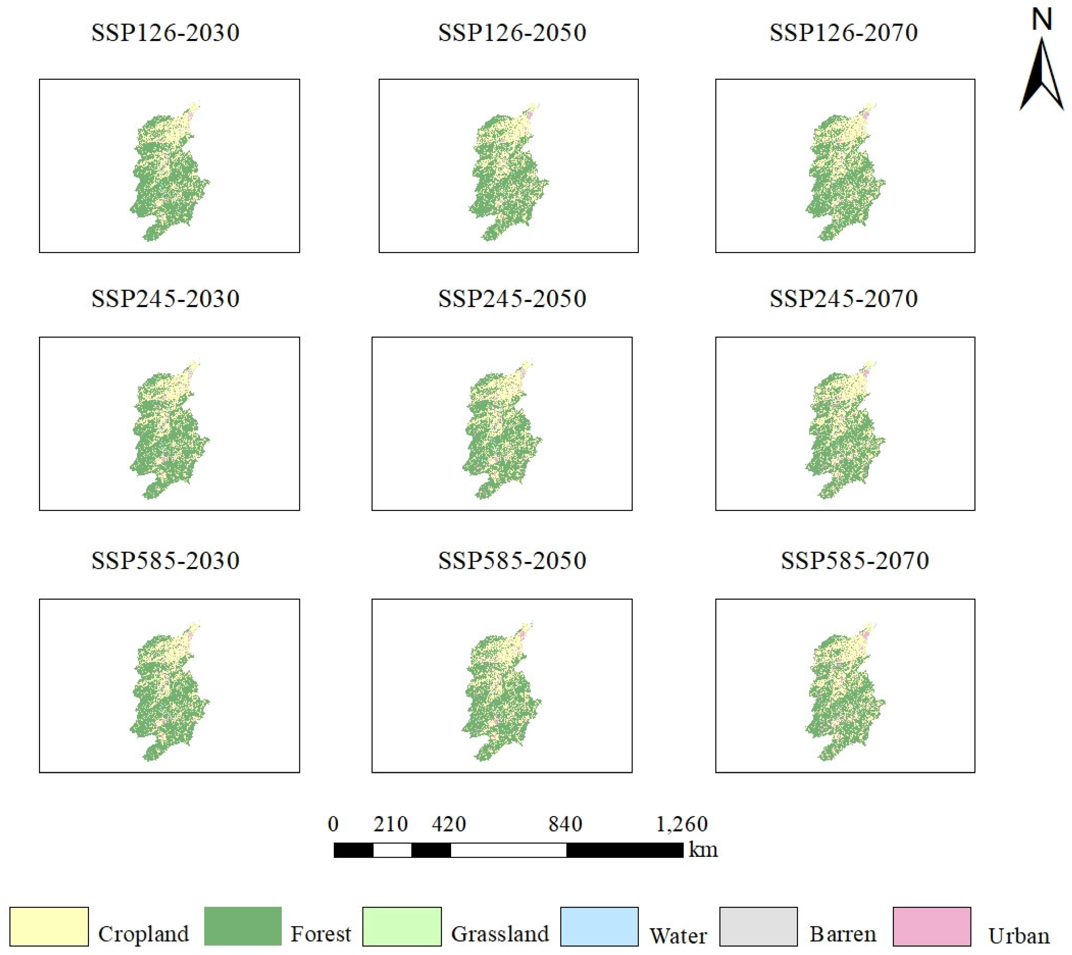
The analysis of land use change projections based on different shared socio-economic pathways (Figure 6) shows that various land use types exhibit significant spatiotemporal evolution characteristics in the future period. As the core carrier of regional agricultural production, arable land shows a stable growth trend in all three scenarios: the growth rate of arable land area remains at around 19.82% in all scenarios by 2030; by 2050, the increase expands to 31.45%; by 2070, it further increases to 38.40%, reflecting the significant effectiveness of policies ensuring food security and measures protecting agricultural land.
Forestland changes exhibit distinct scenario-specific characteristics. Under the SSP1-2.6 low-emission scenario, forestland area decreases by 8%, 12.4%, and 15.05% in 2030, 2050, and 2070, respectively, with relatively moderate reductions. Under the SSP2-4.5 medium-emission scenario, the reduction in forestland is more pronounced, reaching 9.89%, 16.34%, and 18.67%, respectively. Under the SSP5-8.5 high-emission scenario, the reduction rates are 9.81%, 16.01%, and 18.81%, similar to those under the SSP2-4.5 scenario. However, the quantitative reduction in forest cover does not simply represent a conversion of land use types, but rather indicates structural degradation and functional loss of ecosystems associated with deforestation. Once disturbed by human activities, the resilience of tropical monsoon forests is significantly reduced, and the restoration of their original or near-natural state becomes extremely difficult, if not irreversible. The natural succession process of ecosystems requires time scales of decades to centuries, and under conditions of highly fragmented forestland patches and severely impaired habitat connectivity, the probability of successful restoration is extremely low. Especially when forest ecosystems have undergone unprecedented levels of human disturbance, their biodiversity maintenance mechanisms, carbon sequestration functions, and ecological service provision capabilities all face irreversible loss risks. Therefore, based on the principle of preventive conservation, maintaining the integrity and originality of forest ecosystems should be a top priority in land-use planning. This holds significant strategic importance for ensuring the stability and sustainability of regional ecological security patterns.
Grasslands face severe degradation risks under all scenarios. Under the SSP1-2.6 scenario, the area of grasslands decreases steadily by approximately 49% across all time periods. Under the SSP2-4.5 scenario, grassland degradation is more severe, with the reduction rate gradually easing from 70.99% to 68.07%. Under the SSP5-8.5 scenario, grassland changes exhibit complex nonlinear characteristics, with an 89.25% increase by 2030, a 41.98% decrease by 2050, and a significant 68.07% decrease by 2070, reflecting the instability of ecosystems under high-emission scenarios.
The patterns of changes in water area vary by scenario. Under the SSP1-2.6 and SSP2-4.5 scenarios, water area continues to grow steadily, with growth rates maintaining around 5.6% and 5.36%, respectively; while in the SSP5-8.5 scenario, water area shows a continuous decline, decreasing by 11.46%, 23.56%, and 25.27% by 2030, 2050, and 2070, respectively. This trend may be closely related to the frequent occurrence of extreme climate events and changes in the water cycle process.
Land use for construction purposes shows a significant decreasing trend across all scenarios, with reduction rates exceeding 77% in all periods. This phenomenon may be attributed to the tightening of ecological protection policies and the optimization and adjustment of land use structure. The area of unused land shows a significant growth trend under all scenarios. In the SSP1-2.6 scenario, the increase is relatively moderate (16.75–22.05%), while in the SSP2-4.5 and SSP5-8.5 scenarios, the increase is more pronounced, reaching as high as 130.13%, thereby reserving ample spatial resources for future land development and utilization.

3.4. Prediction of Soil Moisture Under Changing Weather Conditions

To systematically assess the spatiotemporal evolution characteristics of soil moisture in the Ganjiang River Basin in the future, this study will couple land use spatial pattern data predicted by the PLUS model for the years 2030, 2050, and 2070 with future climate scenario data from the CMIP6 multi-model ensemble into the SWAT (Soil and Water Assessment Tool) distributed hydrological model. During model configuration, consistency is maintained in soil physical parameters, hydrological response unit delineation, and other key threshold settings to ensure the comparability of results across different scenarios, thereby accurately simulating the interannual variability and seasonal patterns of soil moisture in the basin at three time scales: near-term (2030), medium-term (2050), and long-term (2070).
Based on long-term observational data from hydrological stations in other regions, this study established a comparative analysis framework for annual average soil moisture before and after land use changes. By quantifying the response mechanisms of soil moisture at different development stages to climate change and adjustments in land use patterns, this study delved into the long-term evolution trends of the hydrological cycle process in the watershed. Two sets of comparative experimental designs were established: one considering land use change scenarios (reflecting human activities, such as adjustments in farmland area and changes in forest cover) and another maintaining land use unchanged (considering only climate change effects), to separate and quantify the contribution of different driving factors to soil moisture changes.
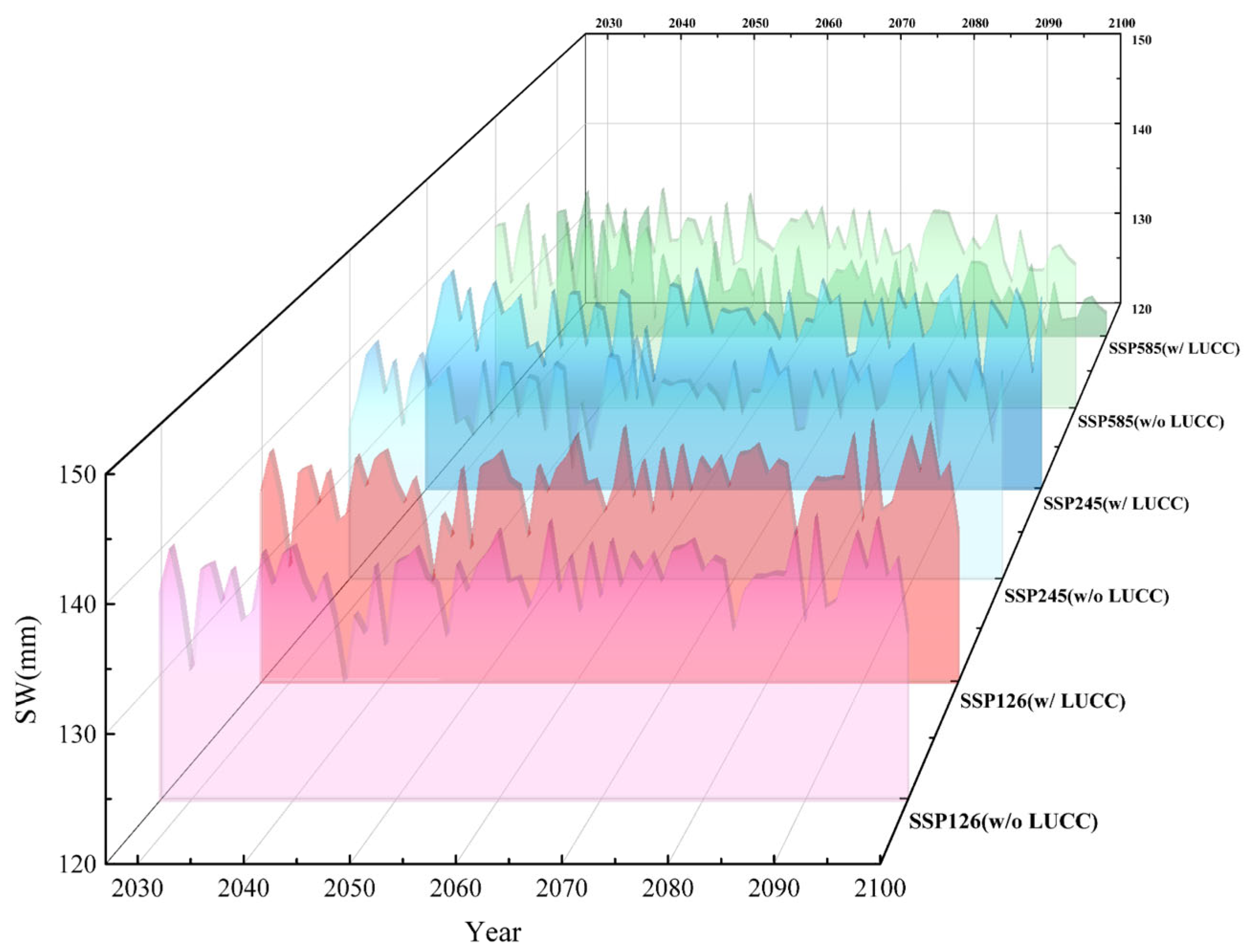
Under the three shared socio-economic pathways (SSP1-2.6, SSP2-4.5, and SSP5-8.5), this study systematically analyzed the differentiated impacts of different emission scenarios on the spatiotemporal distribution of soil moisture in the watershed. By comparing the characteristics of soil moisture changes under scenarios with and without land use changes (see Table 8 and Figure 7), this study provides a scientific basis for accurately assessing the comprehensive impacts of climate change and human activities on watershed hydrological processes. Additionally, it offers important decision-making support for regional water resource management and the formulation of strategies for agricultural sustainable development.
Under different emission scenarios, land use changes exhibit significant scenario-specific and time-dependent effects on soil moisture in the Ganjiang River Basin. In the SSP1-2.6 low-emission scenario, the impact of land use changes on soil moisture is relatively weak and remains stable. During the near-term prediction period (2030), soil moisture content decreases from 137.11 mm to 136.63 mm, with a land use impact change rate of −0.35%; in the medium-term prediction period (2050), it decreases from 136.83 mm to 136.32 mm, with a change rate of −0.37%; and in the long-term prediction period (2070), it decreases from 138.28 mm to 137.75 mm, with a change rate of −0.38%. Under this scenario, the rate of change in land use impact remains within a narrow range of −0.35% to −0.38%, indicating that, under strict carbon emission reduction policies, the disturbance effects of land use pattern adjustments on the hydrological processes of the watershed are relatively mild and tend to stabilize.
Under the SSP2-4.5 medium emissions scenario, the extent of land use change impacts is intensified. During the near-term forecast period, soil moisture content decreases from 137.85 mm to 137.21 mm, with an impact change rate of −0.46%; during the medium-term forecast period, it decreases from 137.10 mm to 136.32 mm, with an impact change rate of −0.57%; and in the long-term forecast period, it decreases from 137.47 mm to 136.72 mm, with an impact change rate of −0.55%. Under this scenario, the impact change rates of land use variation range from −0.46% to −0.57%, showing a stronger negative impact compared to the SSP1-2.6 scenario, reflecting the gradually strengthening weakening effect of land use changes on soil moisture retention capacity under the medium emission pathway.
Under the SSP5-8.5 high emissions scenario, the impact of land use changes on soil moisture is significantly amplified, exhibiting a pronounced time-accumulative effect. During the near-term prediction period, soil moisture content decreases sharply from 135.44 mm to 129.75 mm, with a change rate of −4.20%; during the medium-term prediction period, it drops dramatically from 138.03 mm to 125.67 mm, with the change rate surging to −8.95%; and in the long-term prediction period, it decreases from 137.21 mm to 124.80 mm, with the impact change rate further expanding to −9.04%. Under this scenario, the impact change rate of land use fluctuated within a wide range of −4.20% to −9.04%, and showed a significant deteriorating trend over time, indicating that the drastic adjustment of land use patterns under a high-emission pathway will have profound negative impacts on the hydrological cycle processes in the watershed.
The above analysis results indicate that land use changes have significantly different effects on soil moisture under different emission scenarios: the impact is relatively stable and weak under the SSP1-2.6 scenario, moderate under the SSP2-4.5 scenario, and dramatically amplified with a deteriorating trend under the SSP5-8.5 scenario. This finding provides an important scientific basis for formulating differentiated land use management strategies and water resource protection measures.

3.5. Drought Analysis at Different Scales

3.5.1. SSMI-1 and SSMI-12 Drought Analysis

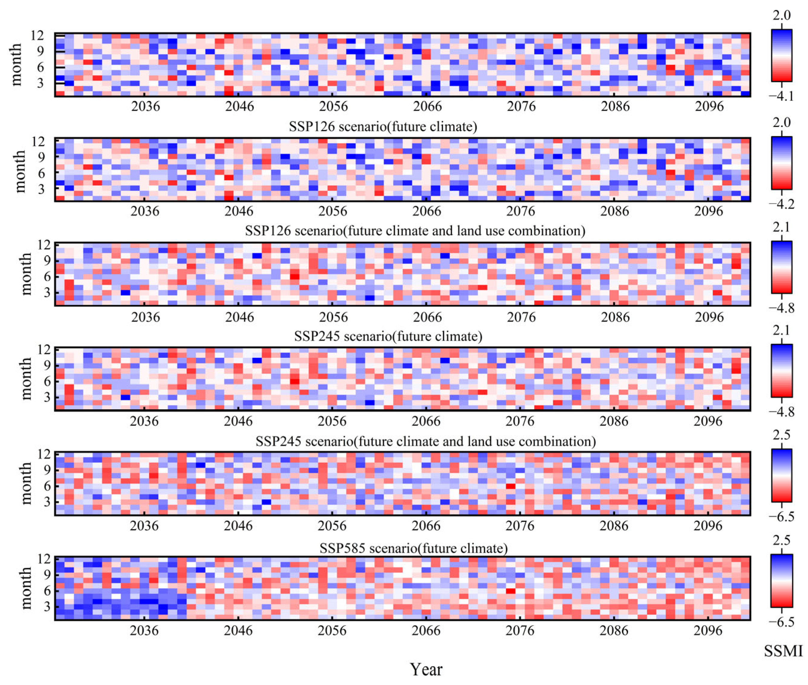
Figure 8 shows the monthly spatiotemporal evolution characteristics of the Standardized Soil Moisture Index (SSMI) under different future emission scenarios, where the SSMI-1 indicator is used to quantify the variability of soil moisture within a year. By comparing the time series distribution patterns of the SSMI under different scenarios, the comprehensive impact mechanism of climate change and land use change on soil moisture conditions in the watershed can be revealed in depth.
Under the SSP1-2.6 low-emission scenario, the SSMI-1 values exhibit a relatively dispersed spatiotemporal distribution pattern, with alternating red and blue blocks in the heat map. This indicates that soil moisture in the Ganjiang River Basin shows significant fluctuations at both interannual and intermonthly scales under this scenario, but lacks obvious long-term trend changes. Notably, large areas of high red values appear in specific years, such as 2046, indicating that soil moisture is relatively abundant during these periods. From a seasonal perspective, the SSMI-1 reaches its peak for the year (1.97) in September–October, with an overall range of −4.15 to 1.97. When land use change factors were included, although the scattered distribution pattern of red and blue blocks remained basically unchanged, some extreme value areas (especially deep red and deep blue areas) underwent significant adjustments, verifying the regulatory effect of land use pattern changes on soil moisture conditions.
Under the SSP2-4.5 medium emissions scenario, the fluctuation characteristics of the SSMI-1 remain significant, and the alternating red and blue distribution pattern persists. However, compared with the SSP1-2.6 scenario, the red high-value areas show a relatively concentrated spatial aggregation trend during the period from 2056 to 2066, and the range of SSMI changes expands to −4.77 to 2.12. The impact of land use changes is more pronounced in this scenario, manifested by a noticeable lightening of the originally deep red areas and corresponding adjustments in the distribution pattern of the blue low-value regions. This indicates that, under the medium emission pathway, the influence of land use changes on soil moisture regulation functions is significantly intensified.
Under the SSP5-8.5 high-emission scenario, the SSMI values exhibit the most pronounced fluctuations, with red high-value areas concentrated in certain regions, particularly during the 2090–2100 period, when the range of SSMI-1 changes sharply expand from −6.48 to 2.52, reflecting the extreme trend in soil moisture conditions under high-emission pathways. Under this scenario, the overall SSMI in the Ganjiang River Basin remains at a relatively high level, but is accompanied by more pronounced temporal variability, indicating the profound impact of frequent extreme climate events on soil moisture cycling processes.
A comprehensive analysis indicates that, from an interannual variability perspective, the SSP1-2.6 scenario exhibits relatively stable but highly fluctuating characteristics; the SSP2-4.5 scenario shows a phenomenon of concentrated high values during certain phases; and the SSP5-8.5 scenario tends toward higher values overall in the later stages with intense fluctuations. From the perspective of intra-annual variation patterns, significant changes in the SSMI are observed in all months, but no obvious seasonal cyclical patterns are identified, reflecting the trend toward increased complexity in the seasonal distribution patterns of soil moisture under future climate conditions. This finding provides important scientific evidence for understanding the nonlinear response mechanisms of hydrological processes in river basins under climate change.
The results of the quantitative assessment of the interannual variability characteristics of agricultural drought based on the 12-month standardized soil moisture index (SSMI-12) are presented in Table 9. This table systematically presents the results for three representative concentration emission pathways (SSP1-2.6, SSP2-4.5, and SSP5-8.5) under three time periods, including the temporal and spatial evolution patterns of drought event frequency, drought occurrence frequency influenced by land use changes, and average drought duration during the three time periods of 2030–2040, 2041–2060, and 2061–2100, and quantitatively analyzed the coupling relationship between land use changes and drought characteristic parameters.
An analysis of drought event frequency indicates that significant phased characteristics are observed under the SSP1-2.6 scenario. During the period from 2030 to 2040, regardless of whether land use changes are considered, the frequency of droughts remainse at 5, indicating that the regulatory effect of land use changes on the frequency of droughts is not yet fully manifested in the early stages of low-emission pathways. As time progresses to 2041–2060, the frequency of droughts increases to 7, reflecting the gradual increase in the probability of droughts driven by climate change. During the period from 2061 to 2100, the frequency of droughts increases significantly, reaching 11 times without considering land use changes and 12 times with land use changes. This phenomenon can be attributed to the cumulative effects of long-term climate change, which significantly increases the frequency of drought events.
Under the SSP2-4.5 scenario, the frequency of droughts exhibits a relatively stable evolution pattern. During the 2030–2040 period, the frequency of droughts is 3 times, a significant decrease compared to the SSP1-2.6 scenario. This may be attributed to the initial inhibitory effect of the climate–land use coupling system on drought events under the moderate emissions pathway. During the 2041–2060 period, the frequency of droughts increases to 5, with a growth trend consistent with SSP1-2.6 but at a relatively moderate rate, indicating that the increase in drought frequency under this scenario exhibits relatively stable characteristics. During the 2061–2100 period, the drought frequency reaches 15 times without considering land use changes and 13 times with land use changes, indicating that land use changes have a certain regulatory effect on drought frequency at the long-term scale but do not alter the overall increasing trend.
Under the SSP5-8.5 scenario, the frequency of droughts exhibits complex nonlinear characteristics. During the period from 2030 to 2040, the frequency of droughts is 5 times without considering land use changes, while it is only 1 time when land use changes are considered, indicating that land use changes have a significant inhibitory effect on drought occurrence in the early stages of high emission scenarios. During the 2041–2060 period, the frequency of droughts is 4 times without considering land use changes, increasing to 8 times when land use changes are considered, reflecting a shift in the mechanism of land use changes’ impact on drought frequency, from an inhibitory effect to a promotional effect. During the period from 2061 to 2100, the frequency of droughts reaches 15 when land use changes are not considered, increasing to 17 when land use changes are considered, which was the highest value among the three scenarios during this period. This indicates that, under the high-emission pathway, the synergistic effects of climate change and land use changes lead to the frequency of droughts reaching an extreme level.
Further analysis of the spatiotemporal evolution characteristics of average drought duration and the moderating effects of land use changes. Under the SSP1-2.6 scenario, during the 2030–2040 period, the average drought duration remainse at 10.4 months regardless of whether land use changes are considered, indicating that land use changes have a negligible effect on drought duration during this period. During the period from 2041 to 2060, the average drought duration under the scenario without considering land use changes is 14.86 months, while it decreases to 14.71 months after considering land use changes. Although the difference was small, it shows a clear downward trend, which may be attributed to the slight mitigating effect of optimized land use allocation on drought duration. Notably, during the 2061–2100 period, the average drought duration under the two scenarios is 7.64 months and 7.17 months, respectively, showing a significant reduction. This phenomenon may reflect the effective regulatory role of long-term climate-adaptive land use strategies and management measures under a sustainable development pathway in controlling drought duration.
Under the SSP2-4.5 scenario, during the period from 2030 to 2040, the average drought duration, adjusted for land use changes, decreases from 14.33 months to 14 months, indicating a negative regulatory effect of land use changes on drought duration. During the 2041–2060 period, although the duration slightly decreases from 15 months to 14.6 months after considering land use changes, it still shows an overall upward trend. This indicates that, under the medium emission scenario, climate-driven factors play a more dominant role in influencing drought duration, while the regulatory capacity of land use changes is relatively limited. During the 2061–2100 period, the drought duration under the two scenarios is 7.93 months and 8.85 months, respectively, significantly shorter than in the previous period. However, the duration after considering land use changes remainse relatively long, revealing the differentiated influence mechanisms of different land use patterns on drought duration at a long-term time scale.
Under the SSP5-8.5 scenario, the evolution pattern of drought duration exhibits more complex characteristics. During the period from 2030 to 2040, land use changes cause the average drought duration to decrease significantly from 14.6 months to 11 months, indicating that land use adjustment strategies implemented in the early stages of the high-emission scenario have a noticeable effect on mitigating drought duration. However, during the 2041–2060 period, although the duration in both scenarios decreases significantly (to 7.75 months and 8.38 months, respectively), the duration slightly increases after considering land use changes, suggesting a directional shift in the regulatory effect of land use changes on drought duration. More notably, during the 2061–2100 period, the drought duration, after accounting for land use changes, surges sharply from 7.67 months to 11.18 months. This phenomenon may reflect that, in the long-term evolution of the high-emission scenario, unreasonable land use patterns exert a significant positive amplifying effect on drought duration, thereby exacerbating the accumulation of drought risks.
Based on the existing research findings, the impact of land use changes on drought frequency and duration exhibits significant spatiotemporal heterogeneity and scenario dependence. In the early stages of this study, land use changes exhibited a certain mitigating effect on drought events, which may be related to improvements in local hydrological processes due to changes in land cover. However, as the time series progressed and global climate change continued to advance, this mitigating effect gradually weakened and even transformed into an exacerbating effect under specific conditions, leading to increased drought frequency and duration. By comparing the simulation results of three typical emission scenarios, it was found that the impact of land use change exhibits significant scenario differences. Under low-emission scenarios (e.g., SSP1-2.6), the positive regulatory effect of land use change is more pronounced over longer time scales, effectively reducing drought occurrence frequency and shortening drought duration. This suggests that, under the premise of effective control of greenhouse gas emissions, reasonable land use management strategies possess significant potential for mitigating drought risks. Conversely, under high emission scenarios (e.g., SSP5-8.5), land use changes may produce negative feedback effects in later periods, exacerbating the intensity and persistence of drought events. This phenomenon may be related to the nonlinear response mechanisms of land–atmosphere interactions under extreme climate conditions.
A comprehensive analysis indicates that the synergistic effects of climate change and land use change on regional drought characteristics exhibit significant multi-scale characteristics, with their mechanisms showing distinct patterns across different emission pathways and time dimensions. This finding highlights that, under the context of global climate change, drought risk assessment and management must fully consider the coupled interactions of the climate–land system and their spatiotemporal evolution patterns.

3.5.2. Trends and Sudden Changes in Land Use Before and After

As shown in Figure 9a–c, this study systematically analyzed the spatiotemporal variation characteristics of the Standardized Soil Moisture Index (SSMI) under different climate scenarios, using the SSMI-3 indicator to reflect the seasonal-scale soil moisture fluctuation patterns. To quantify the driving mechanisms of land use changes on the spatiotemporal evolution of regional soil moisture, this study systematically identified the long-term trends of SSMI-3 under three typical concentration pathways (SSP1-2.6, SSP2-4.5, and SSP5-8.5) using the Mann–Kendall (MK) nonparametric trend test method. Additionally, the Pettitt inflection point test method was employed to precisely locate the significant inflection points in the SSMI-3 series under each scenario. By comparing the test results before and after land use changes, this study delves into the regulatory role of land use/land cover changes in the spatiotemporal patterns of soil moisture evolution and their physical mechanisms, providing a scientific basis for understanding the response mechanisms of hydrological processes under the dual drivers of human activities and climate change.
The statistical analysis results based on the Pettitt test in this study indicate that land use changes under different SSP scenarios exhibit significant differences in their effects on the mutation characteristics of SSMI-3. Under the low-emission SSP1-2.6 scenario, the mutation behavior of SSMI-3 remained highly consistent before and after land use changes, with mutation points accurately located in September 2058 (p < 0.05). This result indicates that land use changes in this scenario did not produce detectable disruptive effects on the timing of the SSMI-3 mutations, revealing the decisive role of climate forcing or other dominant environmental factors in regulating the SSMI-3 mutation mechanism. This stability may be attributed to the relatively mild intensity of land use changes in the SSP1-2.6 scenario, which failed to exceed the critical threshold for influencing soil moisture mutations. The analysis results under the SSP2-4.5 medium-emission scenario showed that mutation points also exhibited temporal synchrony, all occurring in May 2039 (p < 0.05). Although land use changes were more pronounced in this scenario, their modulatory effect on the temporal pattern of the SSMI-3 mutations did not reach statistical significance. However, this apparent temporal consistency does not completely rule out the potential influence of land use changes, as there may be weak signals or nonlinear response mechanisms that have not yet been detected. By contrast, the Pettitt test results under the SSP5-8.5 high-emission scenario exhibit significant divergence. Prior to land use change, the SSMI-3 mutation point was located in April 2073 (p < 0.05); under the land use change scenario, the mutation point shifted significantly forward to August 2040 (p < 0.05), with a time difference of 33 years. This significant advance in mutation timing indicates that high-intensity land use changes in the SSP5-8.5 scenario have profoundly restructured the temporal evolution trajectory of SSMI-3. The physical mechanisms underlying this phenomenon may be closely related to the reorganization of watershed hydrological processes, soil structure alterations, and adjustments in evapotranspiration patterns caused by large-scale land development activities. These factors collectively disrupt the steady state of the soil moisture system, leading to a significant advance in the timing of the transition point. This change pattern poses more severe risks and challenges to regional agricultural sustainable development and ecosystem stability.
The results of the Mann–Kendall trend test under the SSP1-2.6 scenario indicate that, regardless of whether land use change is considered, the UF and UB curves exhibit significant intersection points and show distinct phase-dependent nonlinear fluctuations. In the scenario without considering land use changes, the time series can be identified as having three main significant periods. The first period (2030–2035) exhibits a sharp transition from a significant negative trend (UF value −2.2 to −2.5) to a significant positive trend (peak value 3.42). The second phase (2040–2050) shows alternating positive and negative trends, with UF values reaching a minimum of −2.72 in March 2050. The third phase (2065–2100) exhibits a stable upward trend, with UF values increasing from 2.0 to 5.04. After accounting for land use changes, the trend patterns remain largely consistent, but with adjusted time scales, the first phase is extended to 2030–2042, with a longer duration of the positive trend (UF values ranging from 2.22 to 2.90), the second phase (2047–2050) shows a slight increase in the intensity of the negative trend’s reversal (minimum −2.75), and the third phase (2065–2100) exhibits a more stable growth pattern, with the UF value increasing from 2.04 to 5.07, peaking around 2080, and then maintaining a high range of 4.0–5.0. A comparative analysis indicates that land use changes primarily influence fluctuation cycles and local intensity but do not alter the overall phased change pattern or trend direction.
The results of the Mann–Kendall trend test under the SSP2-4.5 scenario indicate that the time series exhibits significant nonlinear evolution characteristics and complex periodic fluctuations. In the scenario without considering land use changes, the UF curve and UB curve intersect at four significant points. The UF statistic significantly exceeds the ±1.96 confidence level at 60 time points during the analysis period, forming three main significant trend phases: the initial significant increase phase (October 2030 to March 2031) exhibits a strong positive trend, with the UF peak reaching 3.15; the mid-term significant decline phase (March 2041 to October 2044) turnse into a sustained negative trend, with the UF minimum value reaching −2.86; and the late-term sustained decline phase (August 2053 to August 2056) continues the negative trend evolution pattern. After considering land use changes, the overall trend pattern remains consistent but with slightly enhanced fluctuation intensity. The UF and UB curves also exhibit four significant intersection points, with the number of significant time points increasing to 67. The specific manifestations are as follows. The first significant period (October 2030 to March 2031) lasts for six months, with the UF value showing a significant positive trend and the peak increasing to 3.17, reflecting the rapid expansion of land use in the early stages of the SSP2-4.5 scenario. The second significant period (April 2041 to October 2044) spans approximately 3.5 years, with the UF value turning into a significant negative trend and reaching a minimum value of −2.93, indicating a significant slowdown in land use growth. The third significant period (July 2053 to November 2056) lasts approximately 3.3 years, maintaining a negative significant trend, with UF values fluctuating between −1.96 and −2.49. A comparative analysis indicates that the impact of land use changes on trend evolution primarily manifests in localized intensification of fluctuation intensity and minor adjustments to the temporal scale, but does not alter the overall cyclical change pattern or trend transition points.
The results of the Mann–Kendall trend test under the SSP5-8.5 scenario indicate that the time series exhibits significant nonlinear evolution characteristics and complex multi-stage change patterns. Under the scenario without considering land use changes, the UF and UB statistical quantity curves exhibit two significant intersection points. The UF statistical quantity significantly exceeds the ±1.96 confidence level at 253 time points during the analysis period (accounting for approximately 30% of the total duration), forming five major significant trend phases. The initial significant decline phase (October 2030 to April 2038) lasts approximately 7.5 years, with UF values showing a strong negative trend and reaching a minimum value of −4.00, reflecting the rapid decline in land use during the early stages of the SSP5-8.5 scenario. The first recovery phase (August 2052 to September 2057) lasts approximately 5 years, with the UF value turning into a significant positive trend and reaching a peak of 2.36, indicating a phased recovery of land use. The short-term stable phase (February 2060 to December 2061) lasts approximately 2 years, with the UF value maintaining a positive significant level within the range of 1.96 to 2.34; The sustained growth phase (August 2065 to December 2076) is the longest significant period (approximately 11 years), with the UF value peaking at 2.96, indicating that land use enters a long-term growth pattern. The final decline phase (May 2096 to December 2100) lasts approximately 4.5 years, with the UF value again turning into a significant negative trend and reaching a minimum value of −2.97, indicating a significant decline in land use by the end of the 21st century. After considering land use changes, the evolution pattern undergoes a fundamental transformation, with the UF and UB curves having only one significant intersection point and overall exhibiting a single, sustained negative trend characteristic. The UF statistic first exceeds the significance threshold in October 2030 and remainse at a significant level from that year. It reaches a peak during the period from 2034 to 2036 (UF = −3.73), followed by fluctuations but with the trend intensity continuing to strengthen, reaching a value of −10.02 by the end of the study period. This evolution process can be divided into three key stages: the trend establishment phase (2030–2034), during which the UF value rapidly decreases from −2.06 to −3.24, establishing a significant negative trend; the trend intensification phase (2034–2050), during which the UF value continues to fluctuate downward to −6.94, reflecting a significant acceleration in the rate of change; the trend stabilization phase (2050–2100), the UF value fluctuates within the range of −6 to −10, indicating that the negative trend is moderate but remainse highly significant. This single-inflection point pattern combined with a sustained negative trend fully reflects the characteristics of continuous reduction in natural land cover and rapid expansion of artificial land use under the SSP5-8.5 high-emission scenario.

4. Discussion

This study, in the field of climate and meteorology, is based on the CMIP6 climate model framework. It comprehensively analyzes three future climate scenario models—SSP1-2.6, SSP2-4.5, and SSP5-8.5—to systematically assess the drought evolution trends in the Ganjiang River Basin under future climate change and their regional impact mechanisms. The results indicate that the Ganjiang River Basin exhibits significant increases in precipitation and temperature under all climate scenarios. However, the frequency and intensity of drought events also increase synchronously, particularly under the high-emission SSP5-8.5 scenario, where both the number of drought events and their duration show a substantial upward trend. The significant increase in drought risk poses a serious challenge to regional economic development, particularly for the Ganjiang River Basin, where agriculture is a key economic pillar. Agricultural droughts will directly lead to significant crop yield reductions, thereby severely threatening the regional food security system. In-depth research into the evolution patterns and impact mechanisms of agricultural droughts is not only crucial for maintaining the United Nations Sustainable Development Goal of “Zero Hunger”, but provides scientific support for achieving the coordinated and unified objectives of stable production, increased output, and sustainable development. Additionally, water shortages caused by drought will further constrain industrial production and residential water demand, triggering a chain reaction of impacts on regional socio-economic development. Therefore, scientifically predicting drought risks and formulating effective response strategies are of great theoretical significance and practical value for maintaining the sustainable development of the Ganjiang River Basin.
This study employs the PLUS model to conduct a simulation of the future land use pattern evolution in the Ganjiang River Basin. The results indicate that, with the acceleration of urbanization and the continued expansion of industrial parks, the area of unutilized land within the basin exhibits a growth trend, while natural vegetation cover types, such as forestland and grassland, show a reduction trend. Notably, the observed forestland reduction, despite the implementation of China’s ecological protection red line policy, warrants further examination of policy effectiveness and implementation challenges. The apparent contradiction between policy intentions and modeling results suggests several potential factors. First, the ecological red line policy may face implementation gaps at local levels, where economic development pressures could override environmental protection measures. Second, the policy framework, while comprehensive, may require time to demonstrate measurable effects on land use patterns. Third, existing land use trajectories established before policy implementation may continue to influence future scenarios. This fundamental transformation in land use patterns not only significantly alters the physical characteristics of the basin’s land surface and hydrological processes but may also exacerbate the frequency and intensity of agricultural droughts. However, China’s policies on farmland protection and the ecological protection red line system provide an important regulatory framework for land use change. The effectiveness of these policies in preserving forest ecosystems will largely depend on strengthening enforcement mechanisms, improving inter-departmental coordination, and balancing economic development with ecological protection goals. Therefore, when formulating regional drought risk prevention and control strategies, it is essential to consider both policy constraints and their practical implementation effectiveness, ensuring that land use planning optimization aligns with ecological and environmental protection objectives.
The Ganjiang River Basin, as an important agricultural production base in Jiangxi Province, holds a pivotal position in the national food security system. China’s policy of maintaining 1.8 billion acres of arable land as a red line provides an important bottom line guarantee for national food security. It should be implemented through strict arable land protection systems, systematic improvement of arable land quality, and scientific optimization of arable land spatial layout, to build an effective defense system against the risk of food production declines under future climate change. The Ganjiang River Basin currently has 16 large-scale reservoirs and 123 medium-sized reservoirs. These water conservancy infrastructure facilities play a crucial regulatory role in regional drought mitigation and disaster reduction. By establishing a rational reservoir water storage and allocation mechanism, strengthening reservoir operation and management systems, optimizing the scientific allocation of water resources, and advancing the construction of an integrated reservoir water allocation system across the basin, it is possible to effectively alleviate water resource supply and demand conflicts during drought periods. In the face of potentially intensifying drought risks in the future, the Ganjiang River Basin needs to establish a diversified comprehensive drought prevention and response system, with coordinated efforts across multiple dimensions, such as agricultural technological innovation and optimized water resource management. Specific measures should include vigorously promoting efficient water-saving irrigation technologies to enhance agricultural water use efficiency, implementing straw return to fields and other soil moisture conservation techniques to strengthen soil water retention capacity, improving meteorological monitoring and early warning networks to enhance drought early warning accuracy, advancing adjustments to agricultural cropping structures to adapt to climate change trends, and strengthening social publicity, education, and public mobilization to enhance drought prevention awareness across society. Through the systematic implementation of these comprehensive measures, the basin’s overall capacity and adaptability for drought mitigation and disaster reduction will be comprehensively enhanced.
This study achieves theoretical innovation in multi-model integration at the methodological level. Existing coupled model studies mainly have the following limitations: most studies only use a dual-model coupling approach, such as Chen et al. [72], who coupled the SWAT model with a deep learning LSTM model for runoff prediction, and Sun et al. [73], who combined the SWAT model with the CMIP6 climate model to assess the impact of climate change on runoff, but they lack a three-dimensional coupling framework for climate–hydrological-land use. Additionally, existing studies have primarily focused on single temporal scales or spatial ranges. Wang et al. [74] established a SWAT–CMIP6 coupled model for runoff change simulation but did not fully consider the comprehensive impacts of land use changes. By contrast, this study constructed a three-model integration framework of SWAT–CMIP6–PLUS, achieving the following innovative breakthroughs: (1) high-precision simulation capability based on the SWAT hydrological model ensures the reliability of the characterization of basin hydrological processes; (2) integration of the CMIP6 climate prediction model to obtain multi-scenario future meteorological data, providing scientific and reliable driving parameters for the SWAT model; (3) coupling the PLUS land use change simulation model predicts the future spatiotemporal evolution patterns of land use, laying the foundation for agricultural drought and soil water analysis. Through mutual verification and complementary integration among multiple models, a comprehensive theoretical research framework has been established, effectively ensuring the scientific rigor and reliability of the research results.
This study further combines land use change trend analysis with sudden change detection theory, using the Standardized Soil Moisture Index (SSMI) and introducing propagation time theory to systematically reveal the dynamic impact mechanism of land use change on the hydrological cycle process and agricultural drought evolution. This integrated method demonstrates significant innovation in terms of technical means and theoretical foundations, providing new scientific perspectives and technical approaches for regional hydrological cycle and agricultural drought research. Compared with the existing studies, the multi-factor coupling method used in this study fills the gap in the quantitative analysis of the comprehensive impact of soil moisture and agricultural drought changes at the watershed scale. Previous studies on the Ganjiang River Basin have mainly focused on the application of single models. For example, Wang et al. [75] only used multiple precipitation products to drive hydrological models to analyze the hydrological processes in the basin, or simply explored the spatiotemporal distribution patterns of extreme precipitation events. These studies have significant limitations in terms of the depth and breadth of model coupling. Although Liang et al. [76] explored the application of the PLUS model in understanding the drivers of land expansion, the study had a relatively limited time span and lacked a systematic discussion of the dynamic mechanisms by which land use change trends and abrupt changes affect soil moisture and agricultural drought.

5. Conclusions

Firstly, the three core models used in this study all demonstrated good simulation accuracy and predictive capability. In terms of hydrological simulation, the SWAT model, after thorough parameter calibration and validation, demonstrated outstanding performance in simulating runoff in the Ganjiang River Basin. The coefficient of determination (R2) during the calibration and validation periods exceeded 0.75, and the Nash–Sutcliffe efficiency coefficient (NSE) reached above 0.97. These statistical indicators fully validate the applicability and reliability of the SWAT model in simulating hydrological processes in this basin. In terms of land use change prediction, the PLUS model demonstrates good simulation capabilities, particularly in simulating land use spatial patterns under different shared socio-economic pathways (SSP1-2.6, SSP2-4.5, SSP5-8.5). The Kappa consistency coefficients of the models are all greater than 0.75, indicating that the models have high predictive accuracy and reasonable spatial configuration. In terms of climate models, the CMIP6 model ensemble demonstrated robust simulation performance in predicting future climate elements. Temperature simulation results showed that all 15 climate models evaluated performed excellently, with correlation coefficients between the models and the observed data exceeding 0.97 and root mean square errors controlled below 2.98, indicating high simulation accuracy of temperature change trends. In terms of precipitation prediction, the multi-model ensemble mean (MMM-Best) combination, which was selected and optimized, performed the best. Its correlation coefficient with observed precipitation reached 0.72, and the root mean square error was 60.74. The simulation results showed good consistency with observed data, providing high-quality meteorological driving data for the SWAT model’s hydrological simulation.
Secondly, based on the climate change scenario analysis, precipitation and temperature changes in the Ganjiang River Basin under different emission pathways and time periods exhibit distinct spatiotemporal evolution characteristics. During the near-term period (2030–2040), precipitation changes under the three emission scenarios (SSP1-2.6, SSP2-4.5, and SSP5-8.5) are relatively moderate, with an average precipitation of 1582.86 mm, representing a 3.50% increase compared to the baseline period, with a relatively stable growth rate. During the same period, the average temperature is 20.55 °C, a significant increase of 11.96% compared to the baseline period, indicating that the Ganjiang River Basin has entered a distinct warming phase, with temperature changes more pronounced than precipitation changes. The mid-term level years (2041–2060) exhibit significant climate change signals. Under all three scenarios, the average precipitation is 2178.40 mm, a substantial increase of 42.44% compared to the baseline period. Notably, under the SSP1-2.6 scenario, precipitation reaches 3253.63 mm, representing a significant increase of 112.74%. This abnormal growth suggests that the climate system may undergo structural changes during this period. In terms of temperature, the average value is 21.1 °C, an increase of 14.92% compared to the baseline period, with temperature changes showing a steady upward trend. Climate change trends during the long-term reference period (2061–2100) exhibit divergence. The average precipitation is 1676.44 mm, an increase of 9.62% compared to the baseline period. Although it continues to rise, the growth rate slows significantly, exhibiting a relatively stable characteristic compared to the mid-term period. The average temperature reaches 21.91 °C, an increase of 19.35% compared to the baseline period, indicating a sustained warming trend with the warming magnitude gradually expanding. A comprehensive analysis indicates that future climate change in the Ganjiang River Basin exhibits distinct phased characteristics: in the short term, rapid temperature rise is the primary feature; in the medium term, both precipitation and temperature show significant increasing trends; and in the long term, a divergent pattern emerges, with temperatures continuing to rise while precipitation growth slows. This temporal evolution pattern reflects the complexity and nonlinear characteristics of the climate system’s response under different emission scenarios.
Thirdly, based on a spatiotemporal analysis, land use changes in the Ganjiang River Basin exhibit distinct phased characteristics, with the 2000–2010 period showing significant restructuring where arable land, forestland, grassland, and construction land declined markedly, while water bodies and unutilized land expanded, followed by contrasting patterns for the 2010–2020 period, where farmland, water bodies, and unutilized land shifted to significant growth while forestland, grassland, and construction land continued shrinking. These land use transitions significantly impacted soil moisture dynamics, generating an overall declining trend as arable land decreased and unutilized land increased, with impact magnitudes ranging from −4.20% to −9.04% depending on specific transition patterns. The causal mechanisms underlying soil moisture decline operate through multiple pathways: increased impervious surface area reduces precipitation infiltration by converting potential soil recharge into surface runoff, vegetation removal eliminates both root system benefits and litter-enhanced water retention, and hardened surfaces create heat island effects that intensify regional evaporation and accelerate soil water loss. This trend is particularly pronounced under the SSP5-8.5 high-emission scenario, where construction land expansion emerges as the critical driver, demonstrating the strongest negative causal relationship with soil moisture and contributing the primary component of declining effects by systematically altering regional hydrological cycles. However, several uncertainties warrant attention: the 30-m resolution may mask fine-scale heterogeneity in soil moisture–land use relationships, land use scenarios assume unchanged current policy frameworks which may undergo significant changes, and climate model uncertainties may propagate through drought predictions, potentially affecting future risk assessment reliability.
Fourthly, drought indices exhibit significant differences in their fluctuation patterns under different scenarios. Under the SSP1-2.6 scenario, SSMI-1 shows a relatively stable fluctuation pattern, with values ranging from −4.15 to 1.97. Under the SSP2-4.5 scenario, localized high values are observed, with the SSMI-1 value range expanding to −4.77 to 2.12. Under the SSP5-8.5 scenario, the index remainse at a high overall level with intense fluctuations, and the SSMI-1 value range further expands from −6.48 to 2.52. The results of drought event identification based on the SSMI index and travel time theory indicate that the frequency and duration of drought events vary significantly under different emission scenarios and time scales. This study found that, under the high emission scenario (SSP5-8.5), the coupled effects of long-term climate change and land use change significantly increase the frequency of drought events and prolonged their duration. Further analysis indicates that, during the long-term evolution under high emission scenarios, land use changes exert a significant positive influence on drought duration. This phenomenon may be attributed to unreasonable land use patterns exacerbating regional hydrological cycle imbalances, thereby prolonging the duration of drought events.
Finally, a comprehensive analysis using the Mann–Kendall (MK) test and the Pettitt test indicates that land use changes under different climate scenarios have significant differences in their impact on the SSMI-3 mutation characteristics. Under the SSP1-2.6 and SSP2-4.5 scenarios, the timing of the SSMI-3 mutation points remain highly consistent both before and after land use changes. Specifically, all mutation points under the SSP1-2.6 scenario are precisely located in September 2058, while those under the SSP2-4.5 scenario uniformly occur in May 2039. This phenomenon indicates that, under medium- and low-emission scenarios, natural drivers, such as climate change, play a dominant role in the timing control of the SSMI-3 mutations, while the impact of human-induced land use changes is relatively limited. However, under the high-emission SSP5-8.5 scenario, land use changes exert a significant regulatory effect on the timing of the SSMI-3 mutations. Specifically, under current land use conditions, the SSMI-3 mutation point occurs in April 2073; while considering land use changes, the mutation point is significantly advanced to August 2040, with a time span shortened by 33 years. This substantial temporal advancement provides critical early warning capacity for climate adaptation frameworks, which can be summarized as follows: (1) water resource management systems acquire a 33-year lead time for adaptive strategy implementation, encompassing emergency water source establishment, distribution network optimization, and conservation technology integration; (2) agricultural systems obtain adequate preparation intervals for structural crop transitions and irrigation infrastructure modernization through drought-tolerant cultivar deployment, precision irrigation adoption, and cropping system optimization; (3) urban development and infrastructure planning benefit from extended temporal guidance to circumvent high-risk zone development, thereby mitigating socio-economic vulnerability to drought hazards; (4) policy architecture can synchronize land use planning with climate adaptation protocols, leveraging scientific evidence to optimize development sequencing and spatial distribution for soil moisture system mutation risk mitigation. This result reveals that, under extreme climate change, large-scale human land development activities alter surface characteristics and hydrological processes, exerting profound nonlinear impacts on the regional soil moisture cycle system, thereby reshaping the spatiotemporal evolution pattern of drought indices.

Author Contributions

J.W.: conceptualization, methodology, software, data gathering, formal analysis, investigation, validation, writing—original draft preparation, and writing—review and editing. Z.S.: supervision, conceptualization, validation, and writing—review and editing. T.L.: writing—review and editing and data curation. Y.L.: writing—review and editing. L.W.: writing—review and editing. All authors have read and agreed to the published version of the manuscript.

Funding

This project was funded by the National Key R&D Program of China (project number 2022YFD1500402).

Institutional Review Board Statement

Not applicable.

Informed Consent Statement

Not applicable.

Data Availability Statement

The datasets used and analyzed during the current study are available from the corresponding author upon reasonable request.

Conflicts of Interest

The authors declare no conflicts of interest.

References

  1. Tang, R.; Peng, Z.; Liu, M.; Li, Z.-L.; Jiang, Y.; Hu, Y.; Huang, L.; Wang, Y.; Wang, J.; Jia, L.; et al. Spatial-Temporal Patterns of Land Surface Evapotranspiration from Global Products. Remote Sens. Environ. 2024, 304, 114066. [Google Scholar] [CrossRef]
  2. Li, L.; Qian, R.; Liu, W.; Wang, W.; Biederman, J.A.; Zhang, B.; Kang, X.; Wen, F.; Ran, Q.; Zheng, Z.; et al. Drought Timing Influences the Sensitivity of a Semiarid Grassland to Drought. Geoderma 2022, 412, 115714. [Google Scholar] [CrossRef]
  3. Sutanto, S.J.; Van Lanen, H.A.J. Streamflow Drought: Implication of Drought Definitions and Its Application for Drought Forecasting. Hydrol. Earth Syst. Sci. 2021, 25, 3991–4023. [Google Scholar] [CrossRef]
  4. Kyatengerwa, C.; Kim, D.; Choi, M. A National-Scale Drought Assessment in Uganda Based on Evapotranspiration Deficits from the Bouchet Hypothesis. J. Hydrol. 2020, 580, 124348. [Google Scholar] [CrossRef]
  5. Chang, S.; Chen, H.; Wu, B.; Nasanbat, E.; Yan, N.; Davdai, B. A Practical Satellite-Derived Vegetation Drought Index for Arid and Semi-Arid Grassland Drought Monitoring. Remote Sens. 2021, 13, 414. [Google Scholar] [CrossRef]
  6. Damarla, G.; Kavuri, N.C. Comparison of a Decade’s Data between Lst and Ndvi Data for Agricultural Drought Analysis in Rayalaseema Region, Ap, India. IOP Conf. Ser. Mater. Sci. Eng. 2021, 1136, 012009. [Google Scholar] [CrossRef]
  7. Zhang, B.; He, C. A Modified Water Demand Estimation Method for Drought Identification over Arid and Semiarid Regions. Agric. For. Meteorol. 2016, 230–231, 58–66. [Google Scholar] [CrossRef]
  8. Senapati, U.; Das, T.K. Enhancing Agricultural Drought Monitoring with the Integrated Agricultural Drought Index (Iadi): A Multi-Source Remote Sensing Approach. Adv. Space Res. 2025, 75, 8599–8626. [Google Scholar] [CrossRef]
  9. Alahacoon, N.; Edirisinghe, M.; Ranagalage, M. Satellite-Based Meteorological and Agricultural Drought Monitoring for Agricultural Sustainability in Sri Lanka. Sustainability 2021, 13, 3427. [Google Scholar] [CrossRef]
  10. Lee, J.-W.; Hong, E.-M.; Kim, J.-U.; Jang, W.-J.; Jung, C.-G.; Kim, S.-J. Evaluation of Agricultural Drought in South Korea Using Socio-Economic Drought Information. Int. J. Disaster Risk Reduct. 2022, 74, 102936. [Google Scholar] [CrossRef]
  11. Kuwayama, Y.; Thompson, A.; Bernknopf, R.; Zaitchik, B.; Vail, P. Estimating the Impact of Drought on Agriculture Using the Us Drought Monitor. Am. J. Agric. Econ. 2019, 101, 193–210. [Google Scholar] [CrossRef]
  12. Bageshree, K.; Abhishek; Kinouchi, T. A Multivariate Drought Index for Seasonal Agriculture Drought Classification in Semiarid Regions. Remote Sens. 2022, 14, 3891. [Google Scholar] [CrossRef]
  13. García-León, D.; Standardi, G.; Staccione, A. An Integrated Approach for the Estimation of Agricultural Drought Costs. Land Use Policy 2021, 100, 104923. [Google Scholar] [CrossRef]
  14. Wu, B.; Ma, Z.; Yan, N. Agricultural Drought Mitigating Indices Derived from the Changes in Drought Characteristics. Remote Sens. Environ. 2020, 244, 111813. [Google Scholar] [CrossRef]
  15. Dai, M.; Huang, S.; Huang, Q.; Leng, G.; Guo, Y.; Wang, L.; Fang, W.; Li, P.; Zheng, X. Assessing Agricultural Drought Risk and Its Dynamic Evolution Characteristics. Agric. Water Manag. 2020, 231, 106003. [Google Scholar] [CrossRef]
  16. Yin, G.; He, W.; Liu, X.; Xia, Y.; Zhang, H. Wetting or Greening? Probing the Global Trends in Vegetation Condition Index (Vci). Int. J. Appl. Earth Obs. Geoinf. 2024, 129, 103822. [Google Scholar] [CrossRef]
  17. Ren, H.; Du, L.; Peng, C.; Yang, J.; Gao, W. The Composite Drought Index Incorporated Solar-Induced Chlorophyll Fluorescence Enhances the Monitoring Capability of Short-Term Drought. J. Hydrol. 2024, 637, 131361. [Google Scholar] [CrossRef]
  18. Li, M.; Chu, R.; Islam, A.R.M.T. A New Drought Fluorescence Monitoring Index Established for Detecting Drought Evolution Characteristics in the Middle and Lower Reaches of the Yangtze River, China During 2001–2020. IEEE Trans. Geosci. Remote Sens. 2023, 61, 4405613. [Google Scholar] [CrossRef]
  19. Bento, V.A.; Gouveia, C.M.; DaCamara, C.C.; Trigo, I.F. A Climatological Assessment of Drought Impact on Vegetation Health Index. Agric. For. Meteorol. 2018, 259, 286–295. [Google Scholar] [CrossRef]
  20. Muthuvel, D.; Sivakumar, B. Cascading Spatial Drought Network: A Complex Networks Approach to Track Propagation of Meteorological Droughts to Agricultural Droughts. J. Environ. Manag. 2024, 370, 122511. [Google Scholar] [CrossRef]
  21. Fawen, L.; Manjing, Z.; Yong, Z.; Rengui, J. Influence of Irrigation and Groundwater on the Propagation of Meteorological Drought to Agricultural Drought. Agric. Water Manag. 2023, 277, 108099. [Google Scholar] [CrossRef]
  22. Parsons, D.J.; Rey, D.; Tanguy, M.; Holman, I.P. Regional Variations in the Link between Drought Indices and Reported Agricultural Impacts of Drought. Agric. Syst. 2019, 173, 119–129. [Google Scholar] [CrossRef]
  23. Yoon, D.-H.; Nam, W.-H.; Lee, H.-J.; Hong, E.-M.; Feng, S.; Wardlow, B.D.; Tadesse, T.; Svoboda, M.D.; Hayes, M.J.; Kim, D.-E. Agricultural Drought Assessment in East Asia Using Satellite-Based Indices. Remote Sens. 2020, 12, 444. [Google Scholar] [CrossRef]
  24. Nigatu, Z.M.; You, W.; Melesse, A.M. Drought Dynamics in the Nile River Basin: Meteorological, Agricultural, and Groundwater Drought Propagation. Remote Sens. 2024, 16, 919. [Google Scholar] [CrossRef]
  25. Sanchez, N.; González-Zamora, Á.; Martínez-Fernández, J.; Piles, M.; Pablos, M. Integrated Remote Sensing Approach to Global Agricultural Drought Monitoring. Agric. For. Meteorol. 2018, 259, 141–153. [Google Scholar] [CrossRef]
  26. Yu, Z.; Ciais, P.; Piao, S.; Houghton, R.A.; Lu, C.; Tian, H.; Agathokleous, E.; Kattel, G.R.; Sitch, S.; Goll, D.; et al. Forest Expansion Dominates China’s Land Carbon Sink since 1980. Nat. Commun. 2022, 13, 5374. [Google Scholar] [CrossRef] [PubMed]
  27. Jin, G.; Peng, J.; Zhang, L.; Zhang, Z. Understanding Land for High-Quality Development. J. Geogr. Sci. 2023, 33, 217–221. [Google Scholar] [CrossRef]
  28. The Cmip6 Landscape. Nat. Clim. Chang. 2019, 9, 727. [CrossRef]
  29. Abalos, M.; Calvo, N.; Benito-Barca, S.; Garny, H.; Hardiman, S.C.; Lin, P.; Andrews, M.B.; Butchart, N.; Garcia, R.; Orbe, C.; et al. The Brewer-Dobson Circulation in Cmip6. Atmos. Chem. Phys. 2021, 21, 13571–13591. [Google Scholar] [CrossRef]
  30. Grise, K.M.; Davis, S.M. Hadley Cell Expansion in Cmip6 Models. Atmos. Chem. Phys. 2020, 20, 5249–5268. [Google Scholar] [CrossRef]
  31. Zhao, Y.; Sun, D.-Z. Enso Asymmetry in Cmip6 Models. J. Clim. 2022, 35, 5555–5572. [Google Scholar] [CrossRef]
  32. Gier, B.K.; Schlund, M.; Friedlingstein, P.; Jones, C.D.; Jones, C.; Zaehle, S.; Eyring, V. Representation of the Terrestrial Carbon Cycle in Cmip6. Biogeosciences 2024, 21, 5321–5360. [Google Scholar] [CrossRef]
  33. Back, S.-Y.; Kim, D.; Son, S.-W. Mjo Diversity in Cmip6 Models. J. Clim. 2024, 37, 4835–4850. [Google Scholar] [CrossRef]
  34. Nie, Y.; Lin, X.; Yang, Q.; Liu, J.; Chen, D.; Uotila, P. Differences between the Cmip5 and Cmip6 Antarctic Sea Ice Concentration Budgets. Geophys. Res. Lett. 2023, 50, e2023GL105265. [Google Scholar] [CrossRef]
  35. Coburn, J.; Pryor, S.C. Differential Credibility of Climate Modes in Cmip6. J. Clim. 2021, 34, 8145–8164. [Google Scholar] [CrossRef]
  36. Li, X.; Tan, J.; Wang, X.; Han, G.; Qian, Z.; Li, H.; Wang, L.; Niu, G. Responses of Spring Wheat Yield and Growth Period to Different Future Climate Change Models in the Yellow River Irrigation Area Based on Cmip6 and Wofost Models. Agric. For. Meteorol. 2024, 353, 110071. [Google Scholar] [CrossRef]
  37. Wang, Z.; Li, X.; Mao, Y.; Li, L.; Wang, X.; Lin, Q. Dynamic Simulation of Land Use Change and Assessment of Carbon Storage Based on Climate Change Scenarios at the City Level: A Case Study of Bortala, China. Ecol. Indic. 2022, 134, 108499. [Google Scholar] [CrossRef]
  38. Cai, Y.; Zhang, F.; Shi, J.; Johnson, V.C.; Ahmed, Z.; Wang, J.; Wang, W. Enhancing Swat Model with Modified Method to Improve Eco-Hydrological Simulation in Arid Region. J. Clean. Prod. 2023, 403, 136891. [Google Scholar] [CrossRef]
  39. Castaneda-Gonzalez, M.; Poulin, A.; Romero-Lopez, R.; Turcotte, R. Hydrological Models Weighting for Hydrological Projections: The Impacts on Future Peak Flows. J. Hydrol. 2023, 625, 130098. [Google Scholar] [CrossRef]
  40. Castellanos-Osorio, G.; López-Ballesteros, A.; Pérez-Sánchez, J.; Senent-Aparicio, J. Disaggregated Monthly Swat+ Model Versus Daily Swat+ Model for Estimating Environmental Flows in Peninsular Spain. J. Hydrol. 2023, 623, 129837. [Google Scholar] [CrossRef]
  41. Sánchez-Gómez, A.; Martínez-Pérez, S.; Pérez-Chavero, F.M.; Molina-Navarro, E. Optimization of a Swat Model by Incorporating Geological Information through Calibration Strategies. Optim. Eng. 2022, 23, 2203–2233. [Google Scholar] [CrossRef]
  42. Wang, Y.; Zhu, S.; Yuan, L.; Deng, R. An Automatic Parameter Calibration Method for Theswatmodel in Runoff Simulation. RIVER Res. Appl. 2020, 36, 1321–1333. [Google Scholar] [CrossRef]
  43. Rajat; Athira, P. Calibration of Hydrological Models Considering Process Interdependence: A Case Study of Swat Model. Environ. Model. Softw. 2021, 144, 105131. [Google Scholar] [CrossRef]
  44. Lin, X.; Fu, H. Multi-Scenario Simulation Analysis of Cultivated Land Based on Plus Model-a Case Study of Haikou, China. Front. Ecol. Evol. 2023, 11, 1197419. [Google Scholar] [CrossRef]
  45. Xu, L.; Liu, X.; Tong, D.; Liu, Z.; Yin, L.; Zheng, W. Forecasting Urban Land Use Change Based on Cellular Automata and the Plus Model. Land 2022, 11, 652. [Google Scholar] [CrossRef]
  46. Lu, C.; Qi, X.; Zheng, Z.; Jia, K. Plus-Model Based Multi-Scenario Land Space Simulation of the Lower Yellow River Region and Its Ecological Effects. Sustainability 2022, 14, 6942. [Google Scholar] [CrossRef]
  47. Liu, J.; Hou, Y.; Li, F.; Zheng, B.; Chen, Z.; Zheng, F.; Zhang, X.; Yu, R. Land Use Change Projection and Driving Factors Exploration in Hainan Island Based on the Plus Model. Front. Mar. Sci. 2025, 12, 1534508. [Google Scholar] [CrossRef]
  48. te Wierik, S.A.; Cammeraat, E.L.H.; Gupta, J.; Artzy-Randrup, Y.A. Reviewing the Impact of Land Use and Land-Use Change on Moisture Recycling and Precipitation Patterns. Water Resour. Res. 2021, 57, e2020WR029234. [Google Scholar] [CrossRef]
  49. Chen, S.; Yuan, X. The Timing of Detectable Increases in Seasonal Soil Moisture Droughts under Future Climate Change. Earth’s Future 2024, 12, e2023EF004174. [Google Scholar] [CrossRef]
  50. Nepal, D.; Parajuli, P.B.; Ouyang, Y.; To, S.F.; Wijewardane, N. Assessing Hydrological and Water Quality Responses to Dynamic Landuse Change at Watershed Scale in Mississippi. J. Hydrol. 2023, 625, 129983. [Google Scholar] [CrossRef]
  51. Liu, Y.; Fu, C.; Huang, H.; Zheng, S.; Tu, X. Response of Ecosystem Services to Land Use–Land Cover Change in Poyang Lake Basin, China, under Multiple Scenarios. J. Water Resour. Plan. Manag. 2024, 150, 05024007. [Google Scholar] [CrossRef]
  52. Zhang, Y.; Tang, C.; Ye, A.; Zheng, T.; Nie, X.; Tu, A.; Zhu, H.; Zhang, S. Impacts of Climate and Land-Use Change on Blue and Green Water: A Case Study of the Upper Ganjiang River Basin, China. Water 2020, 12, 2661. [Google Scholar] [CrossRef]
  53. Dangol, S.; Zhang, X.; Liang, X.-Z.; Anderson, M.; Crow, W.; Lee, S.; Moglen, G.E.; McCarty, G.W. Multivariate Calibration of the Swat Model Using Remotely Sensed Datasets. Remote Sens. 2023, 15, 2417. [Google Scholar] [CrossRef]
  54. Pignotti, G.; Rathjens, H.; Cibin, R.; Chaubey, I.; Crawford, M. Comparative Analysis of Hru and Grid-Based Swat Models. Water 2017, 9, 272. [Google Scholar] [CrossRef]
  55. Abbas, T.; Hussain, F.; Nabi, G.; Boota, M.W. Uncertainty Evaluation of Swat Model for Snowmelt Runoff in a Himalayan Watershed. Terr. Atmos. Ocean. Sci. 2019, 30, 1–15. [Google Scholar] [CrossRef]
  56. Haleem, K.; Khan, A.U.; Khan, J.; Ghanim, A.A.J.; Al-Areeq, A.M. Evaluating Future Streamflow Patterns under Ssp245 Scenarios: Insights from Cmip6. Sustainability 2023, 15, 16117. [Google Scholar] [CrossRef]
  57. McKee, T.B.; Doesken, N.J.; Kleist, J. The Relationship of Drought Frequency and Duration to Time Scales. In Proceedings of the 8th Conference on Applied Climatology, Anaheim, CA, USA, 17–22 January 1993. [Google Scholar]
  58. Xu, L.; Chen, N.; Yang, C.; Zhang, C.; Yu, H. A Parametric Multivariate Drought Index for Drought Monitoring and Assessment under Climate Change. Agric. For. Meteorol. 2021, 310, 108657. [Google Scholar] [CrossRef]
  59. Krueger, E.S.; Ochsner, T.E.; Quiring, S.M. Development and Evaluation of Soil Moisture-Based Indices for Agricultural Drought Monitoring. Agron. J. 2019, 111, 1392–1406. [Google Scholar] [CrossRef]
  60. Modanesi, S.; Massari, C.; Camici, S.; Brocca, L.; Amarnath, G. Do Satellite Surface Soil Moisture Observations Better Retain Information About Crop-Yield Variability in Drought Conditions? Water Resour. Res. 2020, 56, e2019WR025855. [Google Scholar] [CrossRef]
  61. Tramblay, Y.; Seguí, P.Q. Estimating Soil Moisture Conditions for Drought Monitoring with Random Forests and a Simple Soil Moisture Accounting Scheme. Nat. Hazards Earth Syst. Sci. 2022, 22, 1325–1334. [Google Scholar] [CrossRef]
  62. Dorigo, W.A.; Xaver, A.; Vreugdenhil, M.; Gruber, A.; Hegyiová, A.; Sanchis-Dufau, A.D.; Zamojski, D.; Cordes, C.; Wagner, W.; Drusch, M. Global Automated Quality Control of in Situ Soil Moisture Data from the International Soil Moisture Network. Vadose Zone J. 2013, 12, vzj2012.0097. [Google Scholar] [CrossRef]
  63. Fan, J.; Xu, F.; Sun, X.; Dong, W.; Ma, X.; Liu, G.; Cheng, Y.; Wang, H. Construction and Application of Hydrometeorological Comprehensive Drought Index in Weihe River. Atmosphere 2022, 13, 610. [Google Scholar] [CrossRef]
  64. Wen, Y.; Zhou, L.; Kang, L.; Chen, H.; Guo, J. Drought Risk Analysis Based on Multivariate Copula Function in Henan Province, China. Geomat. Nat. Hazards Risk 2023, 14, 2223344. [Google Scholar] [CrossRef]
  65. Lin, H.; Yu, Z.; Chen, X.; Gu, H.; Ju, Q.; Shen, T. Spatial-Temporal Dynamics of Meteorological and Soil Moisture Drought on the Tibetan Plateau: Trend, Response, and Propagation Process. J. Hydrol. 2023, 626, 130211. [Google Scholar] [CrossRef]
  66. Wang, Y.; Deng, F.; Cai, Y.; Zhao, Y. Spatial and Temporal Change in Meteorological Drought in Gansu Province from 1969 to 2018 Based on Reof. Sustainability 2023, 15, 9014. [Google Scholar] [CrossRef]
  67. Kim, B.S.; Chang, I.G.; Sung, J.H.; Han, H.J. Projection in Future Drought Hazard of South Korea Based on Rcp Climate Change Scenario 8.5 Using Spei. Adv. Meteorol. 2016, 2016, 4148710. [Google Scholar] [CrossRef]
  68. Mohsin, M.; Adnan, S. Probabilistic Modelling of Interarrival Time of Drought for Different Operational Drought Indices Used in Pakistan. Int. J. Climatol. 2023, 43, 6851–6865. [Google Scholar] [CrossRef]
  69. Vergni, L.; Todisco, F.; Mannocchi, F. Analysis of Agricultural Drought Characteristics through a Two-Dimensional Copula. Water Resour. Manag. 2015, 29, 4203–4204. [Google Scholar] [CrossRef]
  70. Vinatier, F.; Arnaiz, A.G. Using High-Resolution Multitemporal Imagery to Highlight Severe Land Management Changes in Mediterranean Vineyards. Appl. Geogr. 2018, 90, 115–122. [Google Scholar] [CrossRef]
  71. Wang, X.; Liu, G.; Xiang, A.; Xiao, S.; Lin, D.; Lin, Y.; Lu, Y. Terrain Gradient Response of Landscape Ecological Environment to Land Use and Land Cover Change in the Hilly Watershed in South China. Ecol. Indic. 2023, 146, 109797. [Google Scholar] [CrossRef]
  72. Chen, S.; Huang, J.; Huang, C., Jr. Improving Daily Streamflow Simulations for Data-Scarce Watersheds Using the Coupled Swat-Lstm Approach. J. Hydrol. 2023, 622, 129734. [Google Scholar] [CrossRef]
  73. Sun, J.; Yan, H.; Bao, Z.; Wang, G. Investigating Impacts of Climate Change on Runoff from the Qinhuai River by Using the Swat Model and Cmip6 Scenarios. Water 2022, 14, 1778. [Google Scholar] [CrossRef]
  74. Wang, S.; Zhang, H.-J.; Wang, T.-T.; Hossain, S. Simulating Runoff Changes and Evaluating under Climate Change Using Cmip6 Data and the Optimal Swat Model: A Case Study. Sci. Rep. 2024, 14, 23228. [Google Scholar] [CrossRef]
  75. Wang, Q.; Xia, J.; Zhang, X.; She, D.; Liu, J.; Li, P. Multi-Scenario Integration Comparison of Cmads and Tmpa Datasets for Hydro-Climatic Simulation over Ganjiang River Basin, China. Water 2020, 12, 3243. [Google Scholar] [CrossRef]
  76. Liang, X.; Guan, Q.; Clarke, K.C.; Liu, S.; Wang, B.; Yao, Y. Understanding the Drivers of Sustainable Land Expansion Using a Patch-Generating Land Use Simulation (Plus) Model: A Case Study in Wuhan, China. Comput. Environ. Urban Syst. 2021, 85, 101569. [Google Scholar] [CrossRef]
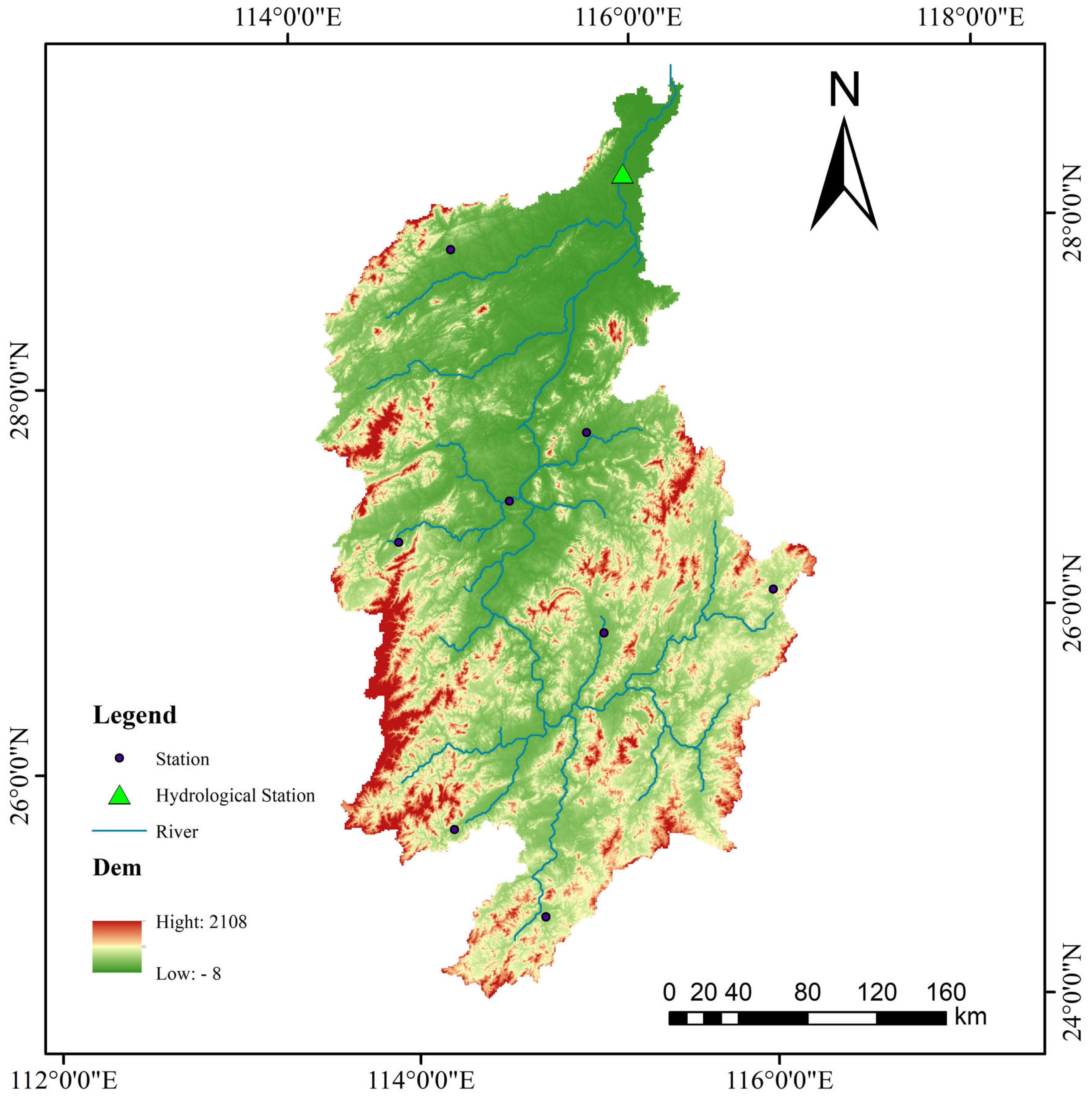
Figure 1. Distribution of water systems and hydrological and meteorological stations in the Ganjiang River Basin.
Sustainability 17 07119 g001
Figure 2. Research framework diagram.
Sustainability 17 07119 g002
Figure 3. Simulation results of the Ganjiang River Basin model.
Sustainability 17 07119 g003
Figure 4. Taylor plots of rainfall, maximum temperature, and minimum temperature in the Ganjiang River Basin from 1970 to 2014 simulated by CMIP6 relative to observation stations. Figure (a) shows the Taylor plot of CMIP6 model precipitation relative to observed data from the reference period; Figure (b) shows the Taylor plot of CMIP6 model maximum temperatures relative to observed data from the reference period; Figure (c) shows the Taylor plot of CMIP6 model minimum temperatures relative to observed data from the reference period.
Sustainability 17 07119 g004
Figure 5. Land use string diagram from 2000 to 2020.
Sustainability 17 07119 g005
Figure 6. Predicted land use distribution map of the Gan River Basin.
Sustainability 17 07119 g006
Figure 7. Analysis of the temporal effects of land use and climate change on soil moisture. Note: w/o LUCC means Without land use change, w/LUCC means With land use change.
Sustainability 17 07119 g007
Figure 8. SSMI maps of land use and future climate under different scenarios (SSP1-2.6, SSP2-4.5, SSP5-8.5).
Sustainability 17 07119 g008
Figure 9. (a) M − K test and p-value inflection point before and after land use under the SSP1-2.6 scenario. (b) M − K test and p-value inflection point before and after land use under the SSP2-4.5 scenario. (c) M − K test and p-value inflection point before and after land use under the SSP5-8.5 scenario.
Sustainability 17 07119 g009aSustainability 17 07119 g009b
Table 1. Data source information.
Data TypeData NameYearData Source
Basic dataA dataset of multi-period remote sensing monitoring of land use in China CNLUCC)2000, 2010, and 2020Chinese Academy of Sciences Center for Resources and Environmental Science and Data (https://www.resdc.cn/, accessed on 1 July 2025)
hydrological station data2020Earth Resources Data Cloud Platform (www.gis5g.com, accessed on 1 July 2025)
Natural elementASTER GDEM V3 (X1)2015Geospatial data cloud (https://www.gscloud.cn/, accessed on 1 July 2025)
slope (X2)Calculated from DEM slope
Distance from water (X3)2015OpenStreetMap
(https://www.openstreetmap.org, accessed on 1 July 2025)
Temperature/forecast (X4)2030, 2050, and 2070Chinese Academy of Sciences Center for Resources and Environmental Science and Data (https://www.resdc.cn/, accessed on 1 July 2025)
Precipitation/future precipitation (X5)CMIP6 database (https://www.nccs.nasa.gov, accessed on 1 July 2025)
Socio-economic factorPopulation/future population (X6)2015,
2030, 2050, and 2070
Chinese Academy of Sciences Center for Resources and Environmental Science and Data (https://www.resdc.cn/, accessed on 1 July 2025)
Scientific data bank (https://cstr.cn/31253.11.sciencedb.01683, accessed on 1 July 2025)
GDP/future GDP (X7)Chinese Academy of Sciences Center for Resources and Environmental Science and Data (https://www.resdc.cn/, accessed on 1 July 2025)
Distance between government seat (city or county level) (X8 and X9)2015National Geographic Information Resources Catalog Service System (https://www.webmap.cn/, accessed on 1 July 2025)
Nature reserve (X10)2015OpenStreetMap
(https://www.openstreetmap.org, accessed on 1 July 2025)
Distance to primary, secondary, and tertiary roads (X11, X12, and X13)
Night light (X14)
Table 2. Overview of the 14 global climate patterns for CMIP6.
Pattern NameCountrySpatial ResolutionPattern NameCountrySpatial Resolution
ACCESS-CM2Australia0.25° × 0.25°EC-Earth3Europe0.25° × 0.25°
ACCESS-ESM1-5IPSL-CM6A-LR
NorESM2-LMNorwayMIROC6Japan
NorESM2-MMMIROC-ES2L
MPI-ESM1-2-HRGermanyMRI-ESM2-0
MPI-ESM1-2-LRGFDL-ESM4United States
INM-CM4-8RussiaCanESM5Canada
Table 3. Domain weights and transfer costs matrix under different scenarios.
Land Use TypeField WeightSSP1-2.6 ScenarioSSP2-4.5 ScenarioSSP5-8.5 Scenario
CFGWBUCFGWBUCFGWBU
C1101101101111100011
F0.416111001010001110001
G0.004101100101111101111
W0.069000100000111100110
B0.001111111111111111111
U0.268000001001001000001
Note: “C” denotes arable land, “F” denotes forestland, “G” denotes grassland, “U” denotes urban land, ‘B’ denotes bare land, and “W” denotes river basins. In the conversion rules for land use and land cover types, the value “1” indicates that a land use and land cover type can be converted to another type; while a value of “0” means that there is no possibility of conversion between different land use and land cover types.
Table 4. Classification of drought conditions.
HorizontalTypeSSMI
1no drought−0.5 < SSMI
2light drought−1 < SSMI ≤ −0.5
3moderate drought−1.5 < SSMI ≤ −1
4severe drought−2 < SSMI ≤ −1.5
5extreme droughtSSMI ≤ −2
Table 5. Parameter values of the SWAT model in the Ganjiang River Basin.
Parameter NamePhysical MeaningOptimal ValueRange
V__RCHRG_DP.gwDeep Aquifer Percolation Fraction0.33 0.22~0.33
V__CN2.mgtSCS Curve Number94.79 92.12~96.96
V__SLSOIL.hruSlope Length for Lateral Subsurface Flow135.00 116.08~150.00
V__GWQMN.gwShallow-Aquifer Return Flow Threshold3595.37 3296.43~4182.17
R__CH_W2.rteMain Channel Width2.72 2.35~3.08
V__RAINHHMX(..).wgn_4Maximum Half-Hour Rainfall in April65.25 56.89~79.96
V__GW_REVAP.gwGroundwater Revap Coefficient0.04 0.04~0.05
R__CH_L1.subTributary Channel Length0.61 0.53~1.53
V__SURLAG.bsnSurface Runoff Lag Coefficient17.87 17.33~19.73
V__SMTMP.bsnSnow Melt Base Temperature−9.07 −2.46
V__CH_K1.subEffective Hydraulic Conductivity in Tributary Channel244.75 215.93~265.41
V__LAT_TTIME.hruLateral Flow Travel Time152.15 108.59~154.32
V__RAINHHMX(..).wgn_7Maximum Half-Hour Rainfall in July61.10 60.77~86.57
R__CH_S2.rteMain Channel Slope−0.26 −0.81
V__TIMP.bsnSnow Pack Temperature Lag Factor0.76 0.70~0.77
V__CH_N2.rteManning’s n Value for Main Channel0.03 0.02~−0.06
V__ADJ_PKR.bsnPeak Rate Adjustment Factor0.93 0.84~0.96
V__ALPHA_BNK.rteBank Storage Recession Constant0.59 0.52~0.61
Table 6. Average annual precipitation change in Ganjiang River Basin in the future. Unit: mm.
Base Period
(1970–2014)
Future
Scenario
Near-Term Horizontal Year (2030–2040)Intermediate Horizontal Year
(2041–2060)
Long-Term Horizontal Year
(2061–2100)
Actual Measured ValuePredicted ValueRate of ChangePredicted ValueRate of ChangePredicted ValueRate of Change
1529.36SSP1-2.61607.815.13%3253.63112.74%1685.4310.21%
SSP2-4.51552.931.54%1626.756.37%1651.007.95%
SSP5-8.51587.833.82%1654.818.20%1692.8910.69%
average value1582.863.50%2178.40 42.44%1676.449.62%
Table 7. Future annual average temperature change in Ganjiang River Basin. Unit: °C.
Base Period
(1970–2014)
Future
Scenario
Near-Term Horizontal Year (2030–2040)Intermediate Horizontal Year (2041–2060)Long-Term Horizontal Year
(2061–2100)
Actual Measured ValuePredicted ValueRate of ChangePredicted ValueRate of ChangePredicted ValueRate of Change
18.36SSP1-2.620.5611.99%20.9313.98%20.9213.93%
SSP2-4.520.3811.03%20.9414.06%21.6617.99%
SSP5-8.520.7212.87%21.4316.72%23.1526.12%
average value20.55 11.96%21.114.92%21.9119.35%
Table 8. Analysis of the effects of climate scenarios and land use change on soil moisture in the Ganjiang River Basin.
Change ScenarioClimate Time
Period
Land Use TimeExcluding Land Use Soil Water Content
(m3/s)
Account for Land Use Soil Water Content (m3/s)Rate of Change in Land Use Impact
SSP1-2.62030~20402030137.11 136.63 −0.35%
SSP2-4.5137.85 137.21−0.46%
SSP5-8.5135.44129.75−4.20%
SSP1-2.62041~20602050136.83 136.32−0.37%
SSP2-4.5137.10136.32−0.57%
SSP5-8.5138.03125.67 −8.95%
SSP1-2.62061~21002070138.28 137.75−0.38%
SSP2-4.5137.47 136.72−0.55%
SSP5-8.5137.21124.80−9.04%
Table 9. Impacts of climate scenarios and land use change on drought characteristics.
Change ScenarioClimate Time PeriodLand Use TimeNumber of Droughts Not Counted for Land UseNumber of Drought Occurrences Factored into Land UseAverage Duration Not Including Land UseAverage Duration of Land Use
SSP1-2.62030~204020305510.410.4
SSP2-4.53314.33 14
SSP5-8.55114.611
SSP1-2.62041~206020507714.86 14.71
SSP2-4.5551514.6
SSP5-8.5487.758.38
SSP1-2.62061~2100207011127.64 7.17
SSP2-4.515137.93 8.85
SSP5-8.515177.67 11.18
Disclaimer/Publisher’s Note: The statements, opinions and data contained in all publications are solely those of the individual author(s) and contributor(s) and not of MDPI and/or the editor(s). MDPI and/or the editor(s) disclaim responsibility for any injury to people or property resulting from any ideas, methods, instructions or products referred to in the content.