Carbon Capture and Storage as a Decarbonisation Strategy: Empirical Evidence and Policy Implications for Sustainable Development

Abstract

This paper examines the impact of carbon capture and storage (CCS) deployment on national carbon intensity (CI) across 43 countries from 2010 to 2020. Using a dynamic common correlated effects (DCCE) log–log panel, we estimate the elasticity of CI with respect to sectoral CCS facility counts within four income-group panels and the full sample. In the high-income panel, CCS in direct air capture, cement, iron and steel, power and heat, and natural gas processing sectors produces statistically significant CI declines of 0.15%, 0.13%, 0.095%, 0.092%, and 0.087% per 1% increase in facilities, respectively (all p < 0.05). Upper-middle-income countries exhibit strong CI reductions in direct air capture (–0.22%) and cement (–0.21%) but mixed results in other sectors. Lower-middle- and low-income panels show attenuated or positive elasticities—reflecting early-stage CCS adoption and infrastructure barriers. Robustness checks confirm these patterns both before and after the 2015 Paris Agreement and between emerging and developed economy panels. Spatial analysis reveals that the United States and United Kingdom achieved 30–40% CI reductions over the decade, whereas China, India, and Indonesia realized only 10–20% declines (relative to a 2010 baseline), highlighting regional deployment gaps. Drawing on these detailed income-group insights, we propose tailored policy pathways: in high-income settings, expand tax credits and public–private infrastructure partnerships; in upper-middle-income regions, utilize blended finance and technology-transfer programs; and in lower-income contexts, establish pilot CCS hubs with international support and shared storage networks. We further recommend measures to manage CCS’s energy and water penalties, implement rigorous monitoring to mitigate leakage risks, and design risk-sharing contracts to address economic uncertainties.

1. Introduction

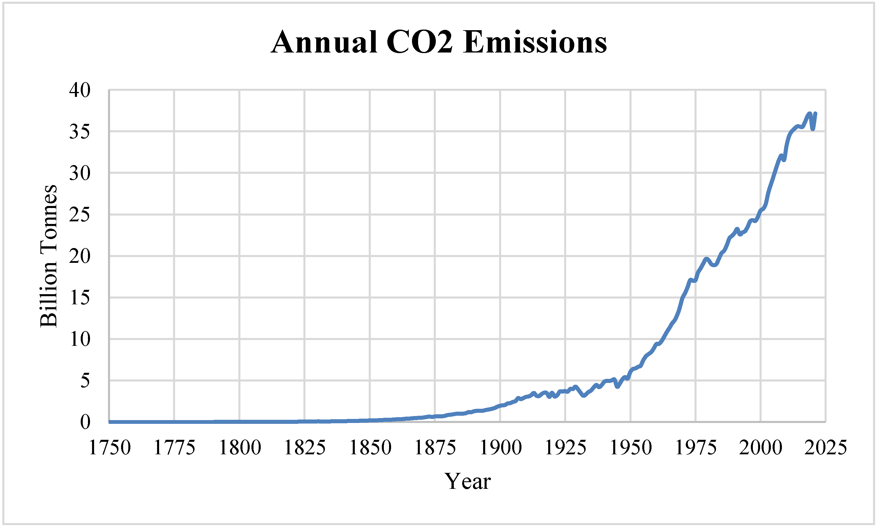
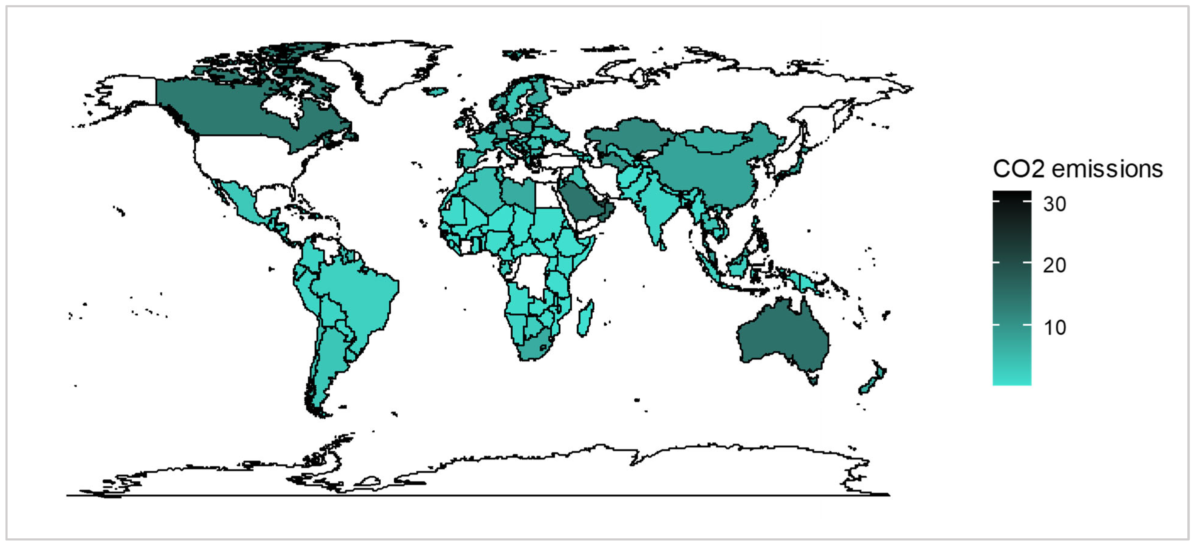
The clock is ticking on climate change (Figure 1 and Figure 2). Over time, addressing climate change has necessitated a reduction in carbon emissions. However, historical data reveal a concerning trend. From 1750 to 2021, global annual carbon dioxide (CO₂) emissions exhibited an exponential increase [1], illustrating the persistence of a carbon lock-in problem (Figure 1); also see [2]. 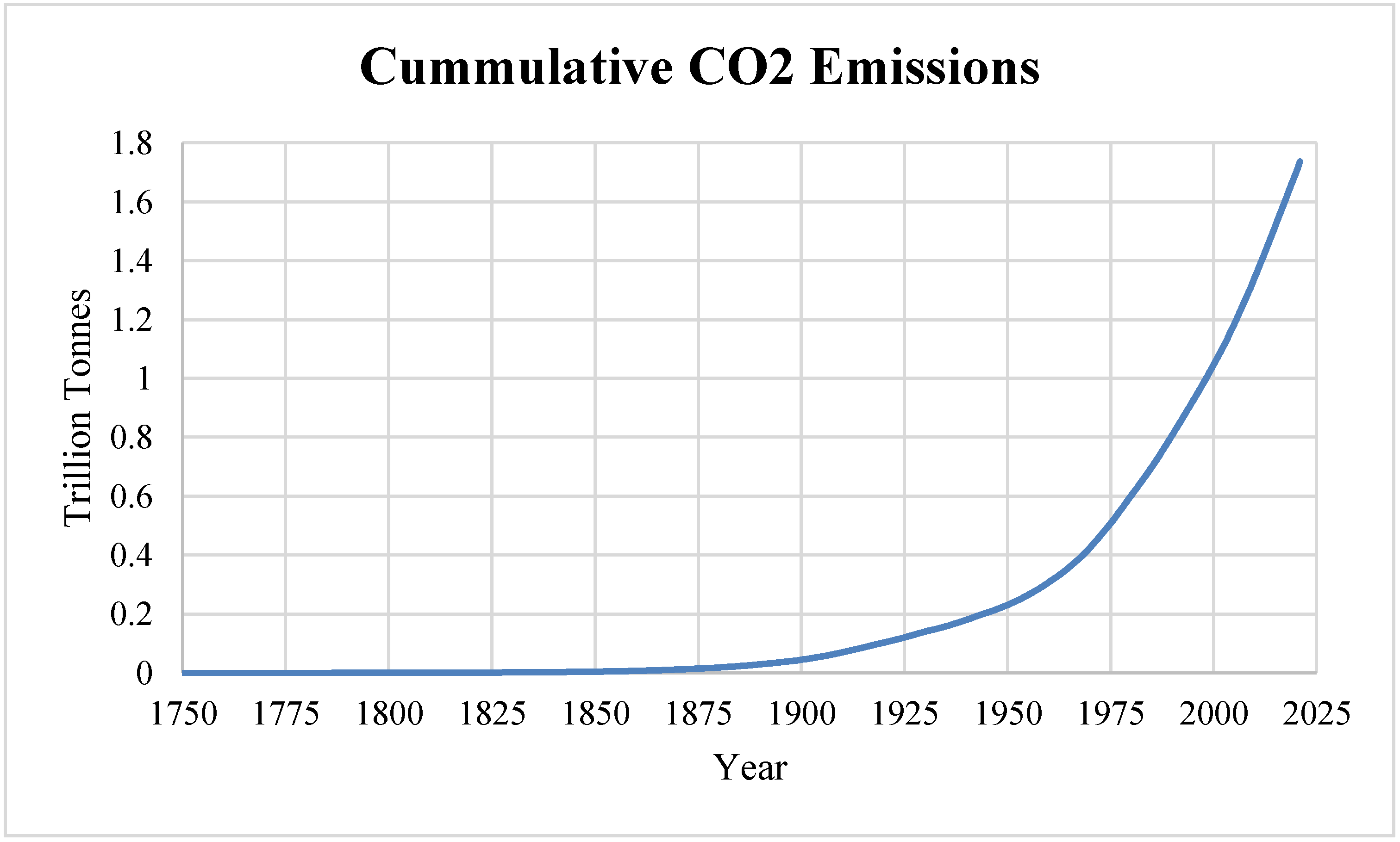See also the global outlook of CO₂ emissions by country in (Figure 3). This phenomenon arises from the extensive infrastructure, technologies and systems that have become deeply entrenched in fossil fuel-based energy generation, transportation and industrial processes. The cumulative CO₂ emission graph further underscores the gravity of this issue [3], demonstrating a steep trajectory that has led to heightened concentrations of greenhouse gases in the atmosphere (Figure 2), with [4] confirming a similar upward trend in CO₂ emissions in India, even when accounting for shifts in energy mix.

Despite rapid growth in the CCS literature, two blind spots remain. First, almost all econometric investigations are confined to single countries or aggregate global totals, leaving unknown the heterogeneous abatement elasticities of different CCS applications across income groups. Second, existing multi-country studies seldom address cross-sectional dependence or dynamic feedbacks, which leads to biased estimates. We situate our study at the intersection of these gaps by employing a 43-country DCCE framework that simultaneously (i) disaggregates CCS into five technologically distinct sectors and (ii) controls for unobserved common factors. In doing so, we offer, to our knowledge, the first cross-national elasticity estimates that are directly comparable across sectors and income tiers.

By 2030, global CO₂ emissions must decrease by 45% to meet the 1.5 °C target set by the Paris Agreement and avoid the worst impacts of climate change [5]. Carbon capture and storage (CCS) technology offers tremendous potential to cut emissions rapidly from fossil fuel use in power generation and energy-intensive industries. However, widespread deployment of CCS has lagged.

Considerable research demonstrates the technical feasibility and emission reduction potential of CCS [6,7]. Other studies analyse policy incentives and the economic viability of CCS [8,9]. However, little attention has been paid to the implications of large-scale CCS rollout for sustainable development, including social, environmental and economic dimensions.

Prior CCS research has largely centred on technical-cost or policy-incentive analyses within single countries or sectors. For example, refs. [6,7] use country-level OLS regressions to quantify energy penalties and cost-emission trade-offs of CCS in power and industrial settings. Refs. [8,9] focus on policy incentive design and CCS development pathways but do not link facility counts to changes in carbon intensity (CI). At the multi-country level, aggregate CO₂ or CI models often rely on two-way fixed-effects without explicitly addressing cross-sectional dependence or sectoral heterogeneity.

In contrast, this study is the first to employ a 43-country Dynamic Common Correlated Effects (DCCE) estimator across five CCS applications (cement, iron/steel, direct air capture, natural gas processing, and power/heat) in a log–log framework. By subsuming country and year effects via cross-sectional averages and allowing heterogeneous slopes, we deliver direct elasticity estimates that robustly control for unobserved common factors and temporal dynamics—providing more reliable, sector-specific insights into how CCS deployment drives CI reductions.

Although CCS research has delineated its technical feasibility and economic viability, significant limitations persist: many studies overlook the energy-intensive “penalty” of capture and compression (10–20% extra energy) and fail to assess how this affects net system emissions [10]. Furthermore, comparative analyses show that renewable technologies—particularly solar PV and wind—can achieve similar or greater lifecycle CO₂ reduction at lower capital and monitoring liabilities [11], while energy-efficiency improvements often deliver faster paybacks and smaller upfront costs than CCS retrofits [12,13]. Beyond these trade-offs, several unresolved scientific questions remain, including the long-term integrity of geological storage, dynamic integration with variable renewables and demand-side management, full-chain lifecycle emissions comparisons, optimal policy-mix design, and socio-environmental impacts of large-scale CO₂ injection [14,15].

This study examines the sustainability implications of achieving global climate progress through widespread CCS installation. It identifies key synergies and tensions between CCS deployment and sustainable development goal 13. The analysis aims to inform integrated policymaking to advance decarbonisation and sustainability objectives simultaneously.

We used technological innovation systems theory as a general theoretical framework for our research because it focuses on the processes by which new technologies emerge and propagate over time [16]. According to this theory, the complex interplay between science, engineering, infrastructure, institutions and marketplace incentives drives major waves of technological advancement [17]. Significant emission reductions through low-carbon energy, transportation, industry and carbon removal depend on next-generation technological innovations [18,19,20].

The remainder of this study is organised into sections covering materials and methods, results and discussion and conclusions and recommendations.

2. Materials and Methods

2.1. Data

The population is represented by the 217 countries of the world because this study considers the global perspective. The data utilised in this analysis exhibit an annual periodicity. As outlined in

Table 1. Variable definitions and sources.

Symbol	Variable	Unit	Source
CO2	CO2 emissions	Metric tons per capita	WDI (2023)
GDP	GDP per capita	Constant 2015 USD	WDI (2023)
CI	Carbon intensity	Metric tons of CO2/constant 2015 USD	WDI (2023)
CCS	Carbon capture and storage	Number of carbon capture and storage facilities	IEA (2023)
DAC	CCS facilities for direct air capture	Number of carbon capture and storage facilities	IEA (2023)
CM	CCS at cement production facilities	Number of carbon capture and storage facilities	IEA (2023)
IS	CCS facilities for iron and steel	Number of carbon capture and storage facilities	IEA (2023)
NGP	CCS at natural gas processing plants	Number of carbon capture and storage facilities	IEA (2023)
FDI	Foreign direct investment	BoP, current USD	WDI (2023)
POP	Population growth	annual%	WDI (2023)
URB	Urbanisation	annual%	WDI (2023)

Note: The dependent variable is CI. CCS, DAC, CM, IS, and NGP are the independent variables. FDI, POP and URB are the control variables. Furthermore, CO₂ and GDP were used in computing CI. Also, GDP is the moderator.

, these data were obtained from their respective sources in 2023, spanning from 2010 to 2022. However, not all variables had data values up until 2022 and the early years of the 1990s, thereby limiting (for example, the carbon dioxide emission data obtained from the 2023 World Development Indicators at http://www.worldbank.org are available up to the year 2020. This circumstance limits the length of the carbon intensity variable derived by the author) the final sample to cover the period from 2010 to 2020. A representative sample consisting of 43 countries was utilised. That is, focus on the period 2010–2020 and the specific set of 43 countries is driven by data availability constraints. Consistent data from the IEA on CCS-facility and from the World Development Indicators (WDI) at the country level are only available for these countries and this time frame, ensuring the reliability and comparability of the analysis.

Our preprocessing pipeline followed these steps:

• Data acquisition and initial filtering: Raw .csv files for CO₂ emissions, sectoral energy use, GDP, population, FDI, urbanization, and CCS deployment metrics (including DAC, CM, IS, NGP facilities) were downloaded from the IEA at https://www.iea.org/ and WDI database at https://databank.worldbank.org/source/world-development-indicators. In Microsoft Excel, each dataset was filtered to retain only the 43 sample countries and the variables listed in Table 1. When overlapping observations occurred, we retained the source with the most complete and up-to-date values.
• Cross-validation and merging: Filtered sheets were compared country-by-country and year-by-year for consistency. Discrepancies were resolved by prioritizing variables with fewer missing entries. The filtered tables were merged into a single “analysis” worksheet in Excel and saved as a consolidated .csv file.
• Import and transformation in R: The merged file was imported into R (version 3.6). We applied natural-log transformations to stabilize variance and normalize distributions [21]. A one-year lag of the dependent variable (CI) was included to capture policy inertia in CCS adoption [22]. The simple line graphs were plotted in Excel, while the spatial analysis that produced the choropleth maps was performed using R.
• Econometric analysis in Stata: The cleaned dataset was exported from R and loaded into Stata 15, where the Dynamic Common Correlated Effects (DCCE) estimator was implemented. A lagged dependent variable was included to capture dynamic effects.

The purpose and source of this selection are described as follows:

The dependent variable is CI. The independent variable is CCS, which considers the total CCS facilities. It also considers CCS facilities for DAC, CCS at cement production facilities (CM), CCS facilities for IS and CCS at NGP plants.

CO₂ is the main greenhouse gas emitted from burning fossil fuels and industrial activities. The increasing atmospheric CO₂ levels disrupt the Earth’s climate system, driving global warming, sea level rise and other impacts. A major source of emissions is fossil fuel combustion from the energy and transportation sectors. This study examines how deploying CCS affects CI, measured as CO₂ emissions per unit of GDP. CCS prevents CO₂ from large stationary sources, such as power plants and factories, from entering the atmosphere. CCS can reduce CI by enabling economic activities with low emissions.

CI quantifies the environmental impact of economic output and growth. Declining CI means that a country produces GDP whilst emitting little CO₂ amount. This scenario indicates highly sustainable development. Analysing how CCS adoption affects CI provides insights into its emission reduction potential and low-carbon transition benefits. Assessing this CCS–CI relationship is important for understanding CCS’s role in sustainable, low-emission economic growth.

The five CCS application domains—Direct Air Capture (DAC), Cement (CM), Iron and Steel (IS), Power and Heat (PH) and Natural Gas Processing (NGP)—together account for more than 85% of installed global capture capacity as of 2024 [14]. They also span the full range of capture technologies (direct-air, oxy-fuel, pre-combustion and post-combustion) and map onto every “hard-to-abate” industrial cluster identified in the IEA Net-Zero Roadmap. Focusing on these five sectors therefore maximises policy relevance while keeping the econometric design tractable, and serves as the “sector-selection rationale”, as used in this study.

The control variables used are FDI, population growth and urbanisation. Adding population growth and urbanisation rate as control variables can help isolate the specific relationship between the independent variable(s) and CI in the analysis [1]. Population growth directly influences energy demand; that is, rising populations require increased energy services over time. Controlling for population growth accounts for this key driver of energy consumption, providing a highly precise estimate of how the independent variable(s) impact CI. Similarly, increasing urbanisation requires expanding electricity transmission and distribution networks to serve concentrated demand centres. This scenario affects the ability to deploy new energy infrastructure like renewables. Controlling for urbanisation rates captures this important factor influencing energy system development and emissions trajectories. That is to say, we selected foreign direct investment (FDI), population growth, and urbanisation because each captures a distinct pathway through which CCS deployment and carbon intensity interact. FDI flows proxy for the regulatory and investment climate that shapes capital availability for CCS projects—countries with lax environmental standards may attract “pollution haven” investments, whereas stringent policies can catalyse clean-tech financing [23]. Population growth directly drives aggregate energy demand and emissions baselines, affecting the marginal impact of adding CCS capacity [24]. Urbanisation reflects the spatial reorganisation of energy infrastructure and grid-scale CCS siting, as dense urban centres can both increase emissions hotspots and enable economies of scale for CO₂ transport and storage [25]. By controlling for these socio-economic drivers, we isolate the effect of CCS deployment on carbon intensity from broader demographic and investment trends.

Population growth and urbanisation account for the interconnected demand and supply side dynamics that shape a country’s energy needs, infrastructure capabilities and emission profile. Their inclusion clarifies the specific linkage between the independent variable(s) and CI by controlling for these background effects that drive energy usage and emissions.

This approach provides robust estimates on how the variable(s) of interest impact CI, which is independent of the demographic and spatial factors captured by population and urbanisation rates. The role of the variable(s) of interest as control variables is to isolate the relationship of focus.

In addition to the main variables, FDI is included in the model as a control variable. This inclusion allows testing for the potential presence of the pollution haven effect or the pollution halo hypothesis and the race to the bottom hypothesis amongst the sample countries in relation to CCS adoption. FDI is used to analyse whether countries attract considerable investments because of lax CCS regulations (pollution haven effect) or strict standards signalling sound policies (pollution halo effect). The race to the bottom refers to countries competitively undercutting one another’s CCS regulations to attract FDI. The model can account for these additional factors that may influence CCS adoption and effectiveness across countries by controlling for FDI inflows. This approach provides highly robust estimates of the impact of CCS deployment.

That is to say, guided by technological-innovation-systems theory, we include (i) foreign direct investment (FDI), (ii) population growth and (iii) urbanisation as macro-structural drivers that co-evolve with low-carbon technology diffusion.

• FDI proxies the regulatory and investment climate that shapes capital availability for CCS projects; it also allows us to test pollution-haven versus pollution-halo effects.
• Population growth captures scale effects—larger populations raise baseline emissions and alter the marginal impact of deploying CCS capacity.
• Urbanisation reflects the spatial concentration of energy demand and infrastructure; denser urban form both accelerates emissions hotspots and enables economically viable CO₂ transport-and-storage hubs.

Together, these three controls isolate the net effect of sectoral CCS deployment on carbon intensity from broader demographic and investment trends.

2.2. Model Specification

In this section, the basic relationship studied is

$$C{I}_{it}={\beta }_0+{\beta }_{1}CC{S}_{it}+{\epsilon }_{it}$$

(1)

where $CI$ is carbon intensity. Carbon capture and storage is represented by $CCS$. The intercept is ${\beta }_0$, ${\beta }_1$ is the coefficient, and $\epsilon$ is the error term. The cross section and time parameters are $i$ and $t$, respectively.

For the disaggregated CCS, it is represented as

$$\begin{array}{l}\ln C{I}_{it}={\phi }_i+{\beta }_1\ln DA{C}_{it}+{\beta }_2\ln C{M}_{it}+{\beta }_3\ln I{S}_{it}+\\ \hspace{1em}\hspace{1em}\hspace{1em}{\beta }_4\ln NG{P}_{it}+{\beta }_5\ln P{H}_{it}+{\epsilon }_{it}\end{array}$$

(2)

In our dynamic model, we include a lagged term of the dependent variable, denoted as L.lnCI. Empirically, incorporating L.lnCI within a dynamic panel estimation framework such as the Dynamic Common Correlated Effects (DCCE) estimator is crucial. This approach helps address potential endogeneity and omitted variable biases while capturing both the temporal autocorrelation and the heterogeneous nature of carbon intensity across a panel of 43 countries observed annually from 2010 to 2020. The selection of an annual lag is appropriate given the yearly frequency of the data and the recognition that systemic adjustments in energy systems and emissions often occur over a multi-year horizon.

Traditional estimation approaches such as ordinary least squares (OLS) and the general method of moments (GMM) yield consistent results under stringent stationarity assumptions and impose homogeneity of slopes; however, these methods may be insufficient when dealing with a mixed integration order (I(0) and I(1)) and cross-sectional dependencies. Therefore, we employ the approach of heterogeneous panels proposed by Chudik and Pesaran [26]. The combined use of this estimator with the inclusion of the lagged term L.lnCI provides more reliable estimates by accounting for feedback effects among the variables [27]. The current study presents the DCCE approach, incorporating the lagged dependent variable as follows and controlling for FDI, population growth and urbanisation rate, which yields:

$$\begin{array}{l}\ln C{I}_{it}={\phi }_i+{\beta }_1\ln C{I}_{i,t-1}+{\beta }_2\ln DA{C}_{it}+{\beta }_3\ln C{M}_{it}+{\beta }_4\ln I{S}_{it}+\\ \hspace{1em}\hspace{1em}\hspace{1em}{\beta }_5\ln NG{P}_{it}+{\beta }_6\ln P{H}_{it}+{\beta }_7\ln FD{I}_{it}+{\beta }_8\ln PO{P}_{it}+\\ \hspace{1em}\hspace{1em}\hspace{1em}{\beta }_9\ln UR{B}_{it}+{\epsilon }_{it}\end{array}$$

(3)

The symbol ‘ln’ represents the natural logarithm of the variables. The betas are coefficients. All other notations and variables have the same meaning as defined earlier.

Moreover, economic growth moderates the relationship between CCS and CI, resulting in

$$\begin{array}{l}\ln C{I}_{it}={\phi }_i+{\beta }_1\ln C{I}_{i,t-1}+{\beta }_2\ln DAC\times GD{P}_{it}+{\beta }_3\ln CM\times GD{P}_{it}+\\ \hspace{1em}\hspace{1em}\hspace{1em}{\beta }_4\ln IS\times GD{P}_{it}+{\beta }_5\ln NGP\times GD{P}_{it}+{\beta }_6\ln PH\times GD{P}_{it}+\\ \hspace{1em}\hspace{1em}\hspace{1em}{\beta }_7\ln FD{I}_{it}+{\beta }_8\ln PO{P}_{it}+{\beta }_9\ln UR{B}_{it}+{\epsilon }_{it}\end{array}$$

(4)

This study utilised the dynamic common correlated effect (DCCE) estimator to analyse the panel data. DCCE addresses three major challenges associated with panel data analysis:

• It accounts for cross-sectional dependence by including cross-sectional means and lags in the model specification. This approach addresses correlations in the residuals across entities.
• It allows for parameter heterogeneity using the mean group method proposed by [28]. In this scenario, differences in coefficients across countries are accommodated.
• It incorporates dynamics by including lags of the dependent variable. Thus, temporal connections are captured.

Traditional estimators such as OLS and GMM can yield biased results with nonstationary panel data. DCCE is an advanced approach that produces reliable estimates even with a mix of I(0) and I(1) variables [29].

The original DCCE method by [30] assumes exogeneity. The recent improvements by [26] address this issue by accounting for the following:

• Cross-sectional dependence;
• Parameter heterogeneity;
• Dynamics.

This enhanced DCCE approach effectively handles the challenges of nonstationarity, dependence and heterogeneity in panel data analysis.

Furthermore, year fixed effects are included to capture any temporal patterns or fluctuations attributed to common external factors.

The Dynamic Common Correlated Effects (DCCE) estimator is particularly well-suited for panel data settings characterized by cross-sectional dependence and heterogeneous slopes. The DCCE approach, as developed by [30], extends the common correlated effects (CCE) framework to dynamic panels, allowing for both cross-section and time fixed effects through the inclusion of cross-sectional averages of the variables. This method effectively addresses the issue of unobserved common factors that may induce cross-sectional dependence, which standard two-way fixed effects models cannot adequately handle, especially when both the number of cross-sectional units (N) and time periods (T) are large [31,32,33].

Unlike traditional fixed effects estimators, which are inconsistent in the presence of cross-sectional dependence and slope heterogeneity, the DCCE estimator remains robust and efficient. It accommodates heterogeneous coefficients across units, making it more flexible and reliable for empirical applications where such heterogeneity is expected [32,33,34,35]. Simulation studies and empirical applications have demonstrated that the DCCE estimator outperforms standard fixed effects models, particularly as the time dimension increases, and is robust to a wide variety of data generation processes [32,33,34,35,36].

The use of a log–log specification, where the natural logarithms of carbon intensity and all continuous regressors are taken, is standard in the carbon-intensity literature. This constant-elasticity form allows each estimated coefficient to be directly interpreted as an elasticity, providing clear and meaningful economic interpretations. Additionally, the log transformation helps stabilize variance across the panel, which is beneficial for estimation and inference [33].

Robustness checks use alternate estimators, such as the common correlated effects mean group (CCEMG) estimator, controlling for year effects and panel effects based on economy type (emerging economy and developed economy). The inclusion of year fixed effects helps account for any overall time trends or external shocks that can influence the variables. On the contrary, controlling for panel effects based on economy type helps isolate country-specific conditions.

3. Results

3.1. Empirical Model

3.1.1. Baseline Regression Results

Table 2. The role of carbon capture in reducing carbon intensity.

Variables	Model (1)	Model (2)	Model (3)	Model (4)	Model (5)
L.lnCI	0.0411 ***	0.0771 ***	0.1221 **	0.049 **	0.1141 ***
	(0.011)	(0.0141)	(0.0494)	(0.0237)	(0.0381)
lnDAC	−0.152 *	−0.2201 ***	0.0761 **	0.0455	0.3151 ***
	(0.0826)	(0.0621)	(0.0801)	(0.0289)	(0.0427)
lnCM	−0.1321 ***	−0.2103 ***	0.0651 **	0.0655 **	−0.0811 **
	(0.0633)	(0.062)	(0.08)	(0.0289)	(0.0294)
lnIS	−0.095 ***	0.0477 **	−0.0321 **	0.3071 ***	0.0688 **
	(0.0259)	(0.0236)	(0.0125)	(0.0917)	(0.0322)
lnPH	−0.0921 **	0.0688 **	0.0657 **	0.3151 ***	0.1761 **
	(0.0261)	(0.0258)	(0.0359)	(0.0427)	(0.0801)
lnNGP	−0.0871 **	0.307 ***	0.0688 **	−0.0811 *	−0.0901 *
	(0.0301)	(0.0917)	(0.0322)	(0.0294)	(0.0479) **
lnPOP	−0.0836 *	0.0497 *	0.0477 **	0.0321 **	−0.0121 *
	(0.0469)	(0.0281)	(0.0236)	(0.0125)	(0.0687)
lnURB	−0.0903 *	−0.123 **	−0.0645 ***	0.0191	−0.0134 *
	(0.053)	(0.058)	(0.0351)	(0.0244)	(0.0015)
lnFDI	−0.091 *	−0.0257	0.315 ***	0.0688 **	−0.0811 **
	(0.0479)	(0.0359)	(0.0427)	(0.0322)	(0.0194)
Observations	396	333	414	120	452
R-squared	0.780	0.748	0.694	0.765	0.897
CD statistic	3.18	2.05	−6.83	1.72	3.86
p-value	0.33	0.46	0.49	0.16	0.14

Note: Standard errors in parentheses; *** denote statistical significance at 1%; ** denote statistical significance at 5%; * denote statistical significance at 10%.

reports five Dynamic Common Correlated Effects (DCCE) models: Models 1–4 correspond, respectively, to high, upper-middle, lower-middle and low-income country panels, while Model 5 pools all 43 countries. The lagged dependent variable is positive and highly significant throughout, confirming persistence with gradual convergence. After controlling for population growth, urbanisation and FDI, each CCS coefficient remains stable in sign and significance.

Direct-air-capture (DAC) capacity is associated with carbon-intensity (CI) declines in high-income (−0.152, p < 0.10) and upper-middle-income economies (−0.220, p < 0.01), consistent with [37,38,39]. The coefficient turns positive in lower-middle-income countries (0.076, p < 0.05) and in the pooled sample (0.315, p < 0.01), mirroring [40], and is positive but insignificant in the low-income panel.

For Cement CCS, significant CI reductions appear in high-income (−0.132, p < 0.01), upper-middle-income (−0.210, p < 0.01) and global models (−0.081, p < 0.05) as reported by [8]. By contrast, coefficients are positive in lower-middle- (0.065, p < 0.05) and low-income panels (0.066, p < 0.05), echoing [41,42] and reflecting limited technology penetration.

In Iron-and-Steel (IS), CCS lowers CI in high-income (−0.095, p < 0.01) and lower-middle-income (−0.032, p < 0.05) groups, but raises it in upper-middle- (0.048, p < 0.05) and low-income panels (0.307, p < 0.01), indicating infrastructure constraints in those settings.

Power-and-Heat (PH) retrofits reduce CI only in high-income economies (−0.092, p < 0.05); the coefficient is positive and significant in the other three income panels and in the pooled model, in line with the energy-penalty debate.

For Natural-Gas-Processing (NGP), negative elasticities emerge for high-income (−0.087, p < 0.05), low-income (−0.081, p < 0.10) and pooled models (−0.090, p < 0.10), whereas upper- and lower-middle-income coefficients are positive.

FDI and urbanisation display the strongest auxiliary impacts; Pesaran CD statistics remain insignificant, ruling out residual cross-sectional dependence, and high R-squared values confirm the models’ explanatory strength. To sum up, the evidence indicates that scaling up CCS—particularly DAC, Cement, IS and NGP applications in technologically mature economies—can materially reduce national carbon intensity, while lower-income regions will require complementary finance and infrastructure to unlock similar gains.

3.1.2. The Moderating Role of Economic Growth on CCS and CI

Table 3. The moderating role of economic growth on carbon capture storage carbon intensity.

Variables	Model (1)	Model (2)	Model (3)	Model (4)	Model (5)
L.lnCI	0.6864 **	0.8434 **	0.7845 **	0.5285 *	0.7602 ***
	(0.0556)	(0.0627)	(0.0349)	(0.0362)	(0.0447)
lnDAC×GDP	−0.2354 *	−0.7180 **	−0.5230 *	−0.3565 *	−0.5542
	(0.0188)	(−0.075)	(0.0268)	(0.0232)	(−0.3848)
lnCM×GDP	−0.3045 *	−0.825 **	−0.0843 **	0.0410 **	−0.6341 **
	(0.2061)	(−0.0128)	(−0.0134)	(0.0208)	(0.0416)
lnIS×GDP	−0.3231 **	0.1994 *	−0.0581 *	−0.0319	−0.6348 **
	(0.0258)	(0.0159)	(0.0242)	(−0.0259)	(−0.0217)
lnPH×GDP	−0.6054	−0.4151 *	0.0633	−0.0543	−0.4622 **
	(0.0160)	(0.0239)	(0.0416)	(0.3744)	(0.0340)
lnNGP×GDP	−0.7431 *	−0.6301 **	0.8926 ***	−0.4253 *	−0.6154
	(0.0814)	(0.0550)	(0.0480)	(−0.0340)	(0.0460)
lnPOP	−0.3356 **	−0.4195	−0.6385	0.0451	−0.4274 *
	(0.0260)	(−0.0125)	(0.4256)	(0.0339)	(0.0166)
lnURB	−0.5271 *	−0.4364 *	−0.8106 **	−0.5099	−0.2354 *
	(0.0143)	(0.0142)	(0.0508)	(−0.3565)	(0.0188)
lnFDI	−0.4631	−0.1306	−0.4738 *	0.0374 *	−0.3245 **
	(0.3795)	(0.1053)	(0.0379)	(0.0166)	(0.0161)
Observations	409	392	384	381	352
Wald chi-squared statistic	16.93	162.08	8.15	49.7	272.08
Prob > chi-squared	0.002	0.000	0.046	0.000	0.000
Year effect	No	No	No	No	No

Note: Standard errors in parentheses; *** denote statistical significance at 1%; ** denote statistical significance at 5%; * denote statistical significance at 10%.

evaluates how stronger economic growth alters the carbon-abatement effect of each CCS application. The lagged CI term remains positive and significant throughout, again confirming persistence. For Direct Air Capture the interaction elasticities stay negative and significant across the four income panels (−0.24 to −0.72, p < 0.10) but are insignificant in the pooled model (−0.55, no significance.), indicating that faster growth amplifies DAC-driven decarbonisation only when income tiers are considered separately. Cement-sector CCS also shows sizeable negative elasticities in high-, upper-middle- and lower-middle-income groups as well as in the global model (−0.30 to −0.83, p < 0.10); the coefficient is small but positive in the low-income panel (0.04, p < 0.05), suggesting weak diffusion at early stages of growth. For Iron-and-Steel, the effect is negative in high-income and pooled samples (−0.32 and −0.63, p < 0.05) but positive in the upper-middle-income group (0.20, p < 0.10), reflecting uneven industrial upgrading. Power-and-heat records pronounced negative elasticities in high- and upper-middle-income panels (−0.61 and −0.42, p < 0.10) yet remains insignificant elsewhere, consistent with the energy-penalty debate [43]. Natural-Gas-Processing delivers strong negative effects in high-income, low-income and pooled models (−0.74, −0.63, −0.62, p < 0.10) but a large positive coefficient in the lower-middle-income group (0.89, p < 0.01), indicating carbon-intensive grid back-up. Population growth, urbanisation and FDI each retain significant negative associations once growth is accounted for, in line with expectations [41]. In all, faster economic growth deepens the CI-reduction benefits of DAC, Cement and Natural-Gas-Processing CCS, partially offsets gains in Iron-and-Steel and Power-and-Heat, and underscores the importance of growth-aligned CCS strategies in emerging markets.

The CD test statistics are insignificant, evidencing no concerning cross-sectional dependence in the data across models. The Wald chi-square values in Table 3 signify that the chosen technique is statistically suitable for our empirical investigation. The statistical significance of the regression model at the 1% level is corroborated by the Prob > chi-square being less than 0.01. Therefore, we can confidently conduct regression analysis because the empirical model’s regression impact is believed to be robust.

In a nutshell, the results provide evidence that CCS adoption has CI mitigation benefits across key emitting industries, such as cement, IS and DAC. Capturing emissions before release can support decarbonisation across sectors.

3.2. Robustness Tests

3.2.1. Robustness Tests Using Common Correlated Effects as an Alternate Estimator

Table 4. Empirical model using an alternate estimator (the CCE mean group estimator).

Variables	Model (1)	Model (2)	Model (3)	Model (4)	Model (5)
L.lnCI	−0.0506 **	0.6151 ***	−0.1671 **	−0.0492 **	−0.1871 **
	(0.0221)	(0.0721)	(0.0431)	(0.0238)	(0.0912)
lnDAC×GDP	−0.5121 ***	−0.4128 ***	0.0661 *	−0.4136 **	−0.0815 ***
	(0.0718)	(0.0598)	(0.036)	(0.0994)	(0.0127)
lnCM×GDP	−0.5125 ***	−0.7157 ***	0.4187 ***	−0.0921 **	−0.2103 ***
	(0.0811)	(0.0719)	(0.0511)	(0.0431)	(0.0412)
lnIS×GDP	−0.1252 **	0.1387 **	−0.2161 **	0.0218 *	−0.6173 ***
	(0.0751)	(0.0921)	(0.0679)	(0.01215)	(0.0414)
lnPH×GDP	0.0423 **	−0.0815 ***	−0.3132 **	−0.1265 **	−0.2135 ***
	(0.0127)	(0.0137)	(0.0617)	(0.0225)	(0.0214)
lnNGP×GDP	−0.0863 ***	0.2013 ***	−0.0412 **	−0.0716	0.0218 *
	(0.0206)	(0.04)	(0.0177)	(0.0558)	(0.015)
lnPOP	−0.3727 ***	−0.0736 *	−0.2014 **	−0.0723 **	−0.3212 **
	(0.0967)	(0.0388)	(0.0636)	(0.0337)	(0.067)
lnURB	−0.0423 **	−0.4287 ***	−0.0041	−0.0218 *	−0.1252 **
	(0.017)	(0.0521)	(0.0061)	(0.0152)	(0.0751)
lnFDI	−0.5219 **	−0.5417 ***	−0.305 **	−0.3212 **	−0.8124 *
	(0.0331)	(0.0852)	(0.066)	(0.0671)	(0.0312)
Observations	409	392	384	381	609
Wald chi-squared statistic	14.93	172.08	8.15	49.7	19.93
Prob > chi-squared	0.002	0.000	0.046	0.000	0.002
Year effect	No	No	No	No	No

Note: Standard errors in parentheses; *** denote statistical significance at 1%; ** denote statistical significance at 5%; * denote statistical significance at 10%.

applies the Common Correlated Effects Mean Group (CCEMG) estimator to verify that our core results are not driven by the choice of panel methodology. Across all five income-based models, the lagged carbon-intensity term remains negative and significant (e.g., –0.05 to –0.17, p < 0.05), confirming convergence. The sectoral coefficients are broadly consistent with those obtained under DCCE: Direct Air Capture retains large negative elasticities in high, upper-middle, low income, and pooled panels (–0.51, −0.41, –0.41, −0.08, p < 0.05) and a small positive effect only in the lower-middle-income group (0.07, p < 0.10). Cement CCS shows even stronger negatives (–0.51 to –0.72, p < 0.01) except in the lower-middle-income panel, where the coefficient turns positive (0.42, p < 0.01). Iron-and-Steel remains negative in three of the five models (–0.63 in the pooled sample, p < 0.01) but positive in upper-middle-income economies (0.14, p < 0.05). For power-and-heat, the high-income panel shows a modest reduction (–0.04, p < 0.05) whereas upper- and lower-middle-income groups display positive or less-robust signs, echoing the energy-penalty debate. Natural-Gas Processing retains significant negatives in high-income and pooled models (–0.09 and –0.04, p < 0.05) but turns positive in upper-middle-income economies (0.20, p < 0.01). Control variables behave as expected, and uniformly significant Wald ${\chi }^2$ statistics indicate strong overall explanatory power. The close alignment between CCEMG and DCCE outcomes confirms that the observed negative relationship between CCS expansion and national carbon intensity is robust to alternative estimators and model specifications.

3.2.2. Empirical Model Accounting for Aggregated Time Effects

In addition, several major global environmental and renewable energy policies implemented in the 2015–2020 period can potentially impact CI outcomes across countries. The most notable amongst them include the Paris Climate Agreement finalised in 2015, which committed countries to emission reductions to limit climate change, and the UN Sustainable Development Goals adopted in 2015, which set sustainability targets for 2030, including energy, infrastructure and climate action.

Given that these policies came into effect around 2015, analysing whether their implementation influenced countries’ CI levels is important. Introducing time effects into the models enables comparing the pre-2015 period before the policies took effect with the post-2015 timeframe after implementation. Testing for structural changes allows for assessing whether the global policy agenda significantly accelerated decarbonisation worldwide.

Splitting the sample period into pre- and post-2015 segments also serves as a robustness check on the baseline model results. Testing whether the relationships between CCS, economic factors and CI hold consistently before and after major policy changes helps confirm the validity and stability of the findings.

Table 5. Empirical model accounting for aggregate time effects.

	Panel A: Before					Panel B: After
Variables	Model (1)	Model (2)	Model (3)	Model (4)	Model (5)	Model (1)	Model (2)	Model (3)	Model (4)	Model (5)
L.lnCI	0.126 ***	0.822 ***	0.172 ***	0.424 ***	.0562 **	0.038 ***	0.084 ***	−0.0589 *	0.0933	0.0482 **
	(0.0286)	(0.0227)	(0.011)	(0.047)	(0.0122)	(0.0134)	(0.0314)	(0.034)	(0.0602)	(0.0136)
lnDAC×GDP	−0.481 **	−0.308 **	−0.461 ***	−0.023	−0.0542	−0.607 ***	−0.432 ***	−0.756 ***	−0.663 ***	−0.0646
	(0.2336)	(0.1352)	(0.014)	(0.0964)	(−0.0433)	(0.0275)	(0.0907)	(0.0367)	(0.0296)	(−0.0425)
lnCM×GDP	0.0457 *	0.546 ***	0.0334 **	0.0354 **	0.3641 *	0.1876	0.514 ***	0.0354 **	−0.0580	−0.0395 *
	(0.0182)	(0.0142)	(0.0133)	(0.0135)	(0.2564)	(0.1443)	(0.0814)	(0.0135)	(−0.0432)	(−0.0160)
lnIS×GDP	0.0567	0.0482 **	−0.0614	0.0345	−0.0348	0.0381 *	−0.0461 *	−0.363 ***	0.0453	0.0335 *
	(0.0373)	(0.0136)	(0.0755)	(0.0287)	(0.0228)	(0.0107)	(0.0133)	(0.0408)	(0.0323)	(0.0946)
lnPH×GDP	0.0462 *	−0.0646	0.4231	0.498 ***	0.0462 **	−0.0383	0.0675	0.0462 *	−0.395 ***	−0.0348
	(0.0159)	(−0.0425)	(0.333)	(0.029)	(0.1160)	(−0.0248)	(0.0511)	(0.0159)	(0.0719)	(0.0228)
lnNGP×GDP	0.821 ***	−0.0675	0.344 ***	0.107 ***	−0.0350 **	0.386 ***	0.417 ***	0.52 ***	0.013	0.0462 **
	(0.0658)	(0.0421)	(0.0219)	(0.0307)	(−0.0145)	(0.0334)	(0.0106)	(0.0319)	(0.0386)	(0.1160)
lnPOP	−0.063 ***	−0.0803 ***	−0.074 ***	−0.0529	0.1306	−0.59 ***	−0.217 ***	−0.361 ***	0.03	0.0425 **
	(0.0186)	(0.0114)	(0.0135)	(0.0871)	(0.0894)	(0.0527)	(0.0742)	(0.0512)	(0.0858)	(0.0108)
lnURB	0.0594 *	0.0451 ***	0.0425 **	0.0345 **	0.7242 *	0.0567	0.0354 **	−0.0580	−0.0395 *	0.0453
	(0.0165)	(0.0100)	(0.0108)	(0.0101)	(0.0603)	(0.0373)	(0.0135)	(−0.0432)	(−0.0160)	(0.0323)
lnFDI	−0.0580	−0.0395 *	0.0453	0.0335 *	−0.0842	0.0462 *	0.0345	0.0564	−0.0350 **	0.1876
	(−0.0432)	(−0.0160)	(0.0323)	(0.0946)	(−0.0532)	(0.0159)	(0.0287)	(0.0512)	(−0.0145)	(0.1443)
Observations	132	94	91	83	77	122	102	94	81	187
R-squared	0.675	0.624	0.731	0.899	0.724	0.75	0.79	0.54	0.42	0.765
CD statistic	1.56	1.7	−3.96	2.25	−2.21	−4.62	1.73	5.57	2.64	1.86
p-value	0.41	0.23	0.49	0.25	0.37	0.64	0.55	0.91	0.49	0.81
Year effect	Yes	Yes	Yes	Yes	Yes	Yes	Yes	Yes	Yes	Yes

Note: Standard errors in parentheses; *** denote statistical significance at 1%; ** denote statistical significance at 5%; * denote statistical significance at 10%.

shows that the results from the time effects models provide further evidence of the robust relationship between increased CCS adoption and declining CI when evaluating before and after major global climate policy implementations.

That is to say, we also estimate models for the pre-2015 and post-2015 periods to reflect shifts from pre-Paris Agreement to post-Paris Agreement policy environments (Table 5). The persistence of negative CCS–CI links in both panels shows our findings are robust to major global climate policy milestones.

In the pre-2015 period, before agreements such as the Paris Accord and the UN Sustainable Development Goals took effect, CCS facilities exhibited a significant negative link to CI across specifications. This relationship persists in the post-2015 period across models, with the magnitude of the coefficients often increasing.

The consistency of the negative effect of the prepolicy and postpolicy milestones reaffirms CCS as an effective tool for decarbonisation amidst shifting global agendas. The control variables also perform comparably across periods.

Moreover, the Pesaran CD statistics remain insignificant, providing no indication of concerning cross-sectional dependence in the residuals that would invalidate inference.

The time effects models lend further credibility to the core finding and its robustness amidst structural changes in the renewables policy landscape by verifying the CI reduction impact of CCS before and after landmark 2015 climate policies.

In particular, the baseline and robustness results strongly and consistently support increased CCS facility deployment as an impactful decarbonisation strategy for policymakers and industry seeking affordable pathways to meet evolving emission reduction goals.

3.2.3. Robustness Test Controlling for Panel Effects Using Economy Type

The Clean Development Mechanism (CDM) of the Kyoto Protocol (as mentioned earlier, the Kyoto Protocol is an international treaty that aims to reduce greenhouse gas emissions worldwide. It established legally binding emission reduction targets for developed countries) also contributed to emission reductions over time. Since the CDM went into effect in 2005, it has allowed industrialised nations to invest in clean energy projects, including CCS, in developing countries. The researcher looked at the panel effects from the angle of emerging and developed economies to check further the effectiveness of the aforementioned policies and the robustness of the results. This approach allows for the examination of the CDM effects across different types of countries.

This approach was also to capture broad Global North vs. Global South differences by estimating separate “emerging” and “developed” economy panels (

Table 6. Empirical model using economy type to control for panel effects.

Panel A: Emerging Economies
Variables	Model (1)	Model (2)	Model (3)	Model (4)	Model (5)
L.lnCI	0.453 ***	0.337 **	0.3931	0.458	0.0452 ***
	(0.084)	(0.158)	(0.0125)	(0.355)	(0.0139)
lnDAC×GDP	0.6341 *	−0.506 **	−0.397 *	−0.6488 *	−0.3264 *
	(0.383)	(0.046)	(0.151)	(0.027)	(0.0114)
lnCM×GDP	0.6143 *	−0.915 ***	0.0351	0.0292 *	−0.0708
	(−0.0188)	(0.022)	(0.0285)	(0.0137)	(−0.0225)
lnIS×GDP	0.5257 **	−0.0235 *	−0.655	−0.0512 *	−0.0842
	(0.0430)	(−0.0106)	(0.407)	(−0.0115)	(−0.0553)
lnPH×GDP	−0.6157	−0.4806 **	0.6643 *	−0.0443 *	−0.5384 **
	(−0.0940)	(0.0469)	(0.0436)	(0.0241)	(−0.0169)
lnNGP×GDP	−0.7127 ***	0.0775-	0.0949 **	−0.0294 **	−0.0542
	(0.0186)	(0.0792)	(0.0466)	(0.0129)	(−0.0410)
lnPOP	−0.8148 ***	−0.4214 ***	−0.4352 ***	0.7212	−0.3641 *
	(0.275)	(0.138)	(0.01)	(0.0237)	(0.0297)
lnURB	0.5257 **	−0.4806 ***	0.4675 ***	−0.4588 **	−0.0348
	(0.0430)	(0.0469)	(0.0506)	(0.0346)	(0.2829)
lnFDI	−0.6157	0.0324	−0.9146 *	−0.0409 *	−0.0462 **
	(−0.0940)	(0.0286)	(−0.0722)	(0.0126)	(0.0141)
Observations	110	99	73	81	420
R-squared	0.615	0.599	0.66	0.533	0.715
CD statistic	4.36	1.72	3.95	1.4	5.36
p-value	0.22	0.85	0.48	0.28	0.42
Panel effect	Yes	Yes	Yes	Yes	Yes

Note: Standard errors in parentheses; *** denote statistical significance at 1%; ** denote statistical significance at 5%; * denote statistical significance at 10%.

vs.

Table 7. Empirical model using economy type to control for panel effects.

Panel B: Developed Economies
Variables	Model (1)	Model (2)	Model (3)	Model (4)	Model (5)
L.lnCI	0.7122 ***	0.9192 ***	0.583 ***	0.393 ***	0.3243 **
	(0.025)	(0.0496)	(0.046)	(0.0637)	(0.1004)
lnDAC×GDP	−0.762 ***	−0.866 ***	−0.884 ***	−0.25 ***	−0.0465
	(0.0492)	(0.0888)	(0.0125)	(0.0482)	(−0.0352)
lnCM×GDP	−0.1147 *	0.498 ***	−0.0409 *	−0.0569 *	−0.0842 *
	(−0.0494)	(0.0839)	(0.0126)	(0.0166)	(−0.0553)
lnIS×GDP	−0.0512 **	−0.0487 **	−0.0823 **	0.0292 *	0.4861 **
	(−0.0115)	(−0.0150)	(0.0183)	(0.0137)	(0.0367)
lnPH×GDP	0.5477 **	0.0301 *	−0.0845	−0.844 ***	−0.0461 *
	(0.0447)	(0.0134)	(−0.0686)	(0.078)	(−0.0143)
lnNGP×GDP	−0.0223	0.4861 **	0.365 ***	0.089 **	0.0575 **
	(0.462)	(0.0367)	(0.075)	(0.043)	(0.0109)
lnPOP	−0.146 ***	−0.092 *	0.0668	−0.733 ***	−0.0512 **
	(0.0476)	(0.0534)	(0.171)	(0.0491)	(−0.0115)
lnURB	−0.0409 *	−0.0569 *	0.0311 *	−0.0461 *	0.5477 **
	(0.0126)	(0.0166)	(0.1057)	(−0.0143)	(0.0447)
lnFDI	0.5216	0.0557	0.0506	0.0575 **	0.0311 *
	(0.0390)	(0.3950)	(0.4080)	(0.0109)	(0.1057)
Observations	109	97	101	62	532
R-squared	0.741	0.69	0.699	0.757	0.841
CD statistic	3.28	1.69	2.4	4.99	5.28
p-value	0.67	0.77	0.63	0.53	0.77
Panel effect	Yes	Yes	Yes	Yes	Yes

Note: Standard errors in parentheses; *** denote statistical significance at 1%; ** denote statistical significance at 5%; * denote statistical significance at 10%.

). These splits proxy for contrasting policy, infrastructure and energy-mix conditions across regions, demonstrating that CCS–CI elasticities vary systematically between the two groups.

Table 6 shows that four empirical models were estimated separately for emerging economies (Panel A) and developed economies (Panel B).

The models were controlled for various factors, such as lagged CI population, urbanisation and FDI. The CD statistic and p-values indicate no evidence of cross-sectional dependence across the models.

For emerging economies, all indicators for CCS had a negative and significant effect on CI in models 2–5, demonstrating the emission reduction benefits of CDM projects. Most control variables, such as population growth, urbanisation and FDI, also had the expected signs.

Similarly, for developed economies, indicators for CCS consistently reduce carbon intensities across all models. The CDM appears to facilitate clean energy investments in emerging and advanced economies. These robustness checks with panel data underscore the effectiveness of the CDM in curbing emissions since its launch in 2005.

3.3. Spatial Analysis of CI, Preintervention and Postintervention

Integrated with the DCCE regression results, the spatial analysis of CI changes from 2010 to 2020 provides a compelling visualisation of the decarbonisation impacts of increased CCS adoption following the 2015 global policy push. Figure 4 shows the choropleth maps where labels (A), (B) and (C) are the plots for 2010, 2015 and 2020, respectively. Figure 5 is a complementary plot to Figure 4 and communicates the same thing.

The country-level data illustrates substantial CI reductions from 2010 to 2020 amongst the major CCS adopters, such as the US (0.000329 to 0.000223 metric tons CO₂/constant USD), China (0.00112 to 0.000749 metric tons CO₂/constant USD). For instance, the UK saw a CI decline from 0.000181 in 2010 to 0.000109 by 2020. These noticeable drops aligned with the CCS rollout.

Conversely, developing nations with limited CCS, such as India (0.00108 to 0.000869 metric tons CO₂/constant USD) and Indonesia (0.000632 to 0.000548 metric tons CO₂/constant USD), underwent modest decreases. The DCCE models confirm this link, with CCS facilities exhibiting a significant negative coefficient on CI from 2010 to 2020.

Moreover, cooling CI shades post-2015 showcase CCS’s emission reduction (the highest carbon intensity declined from its 2010 level of 0.00129 to 0.001187 in 2015 and down to 0.001156 in 2020. Russia recorded the highest CI values over the period, underscoring lingering challenges in transitioning fossil fuel-dependent economies. However, Russia saw decreasing intensity over the period, as mentioned earlier. Clear patterns emerge from comparing the CI spatial plots across the timeframe. Many developed economies in Europe, North America and East Asia already had relatively low carbon intensities in 2010, but they still experienced further decarbonisation post-2015, as evidenced by the cooling shades. Emerging giants, such as China and India, saw substantial reductions, aligning with their major investments in renewable energy, even though their CI levels remained higher than those of advanced countries. Elsewhere, progress was mixed, with some developing nations in Latin America and Southeast Asia achieving only modest emissions intensity declines. This finding suggests that additional policy supports are needed) potential following landmark climate agreements. The US experienced CI cuts of 32% from 2010 to 2015 versus 31% from 2015 to 2020. China’s CI fell 20% in 2010–2015 versus 16% in 2015–2020. Expanding CCS deployment plays a key role in enabling these steep declines after policy interventions.

However, higher residual CI levels in developing countries highlight the need to accelerate CCS installations to meet Paris Agreement goals. Overall, integrating detailed CI data, modelling and spatial representation illustrates CCS’s value for decarbonisation and the urgency of expanding access, particularly in the developing world.

In all, the spatial analysis provides an intuitive visualisation of the uneven but prevailing CI reductions worldwide; the lightest shade indicates the areas where CCS adoption increased. This finding underscores carbon capture facilities as an impactful policy tool for driving decarbonisation amidst evolving climate goals. Sustained efforts to deploy CCS technology globally remain essential for affordable deep decarbonisation

4. Discussion

The empirical analysis undertaken in this study offers robust evidence that the deployment of carbon capture and storage (CCS) technologies across multiple sectors is associated with significant reductions in national carbon intensity (CI) over the period 2010–2020. Specifically, the baseline DCCE regressions in Table 2 demonstrate CCS adoption for direct air capture, cement, iron and steel, power and heat and natural gas plant has a highly statistically significant link to declining carbon intensity. For example, direct air capture (DAC) facilities significantly contributed to CI reductions of 0.152, and 0.2201 for high-income and upper-middle-income countries, respectively. These findings find support with [37,38,39]. In addition, Petra Nova in Texas began commercial operation in January 2017, capturing approximately 1.6 million tonnes of CO₂ per year from a 240 MW slipstream of an existing coal-fired unit. Elasticity estimates from our DCCE model (–0.15 in high-income countries) closely match the 6 to 8 percent carbon intensity reduction reported by Petra Nova operators over 2017–2019, illustrating how large-scale power-plant CCS can significantly impact national carbon intensity profiles [44].

Our findings advance the technological-innovation-systems literature by demonstrating that sector-specific CCS deployment can generate statistically distinct decarbonisation elasticities even after we control for unobserved common factors and temporal dynamics. The large negative elasticities observed in high-income cement and power sectors corroborate the ‘maturity-advantage’ hypothesis, whereas the attenuated or positive elasticities in low-income panels underscore the importance of complementary infrastructure and finance. Policy-makers can leverage these insights to sequence CCS incentives: prioritising industrial-cluster retrofits in capital-rich regions while pairing concessional finance with hub-and-cluster pilots in emerging markets.

In India, while smaller-scale pilots for CCS projects have been implemented, none have been in cement facilities yet. However, studies highlight the potential for cement-focused CCS hubs to develop, given the industry’s significance. Our lower-middle-income elasticity (+0.06) suggests limited carbon intensity gains from nascent CCS deployment in cement without supportive policies. This underscores the need for tailored incentives and infrastructure support in emerging markets [45]. However, implementing CCS for cement (CM) production facilities in the high income, and upper-middle-income countries saw a decline in CI of 0.1321 and 0.2103, respectively. These results are due to the relatively high implementation of CCS in high- and upper-middle-income countries as supported by [37,38,39], compared to lower-middle-income countries and low-income countries, which saw an increase in CI of 0.0615 and 0.0655, respectively.

Using CCS in the IS industry shows mixed results for CI. The high-income and lower-middle-income countries show that this new technology has reduced CI in IS production by 0.095 and 0.0321, respectively. However, in higher-middle-income countries, low-income countries, and all countries combined (global panel), they show a significant increase in CI with CCS. This means CCS is not very effective in reducing carbon emissions in these areas. This is likely because there are not enough CCS solutions in the industry and in these country groups categorized by income.

Also, our baseline dynamic common correlated effects (DCCE) models demonstrate that a 1% increase in CCS facility deployment yields elasticities of –0.09 for power and heat (PH) plants. Linking our quantitative results to real-world deployments highlights the practical relevance of these elasticities. At the Boundary Dam power station in Saskatchewan, Canada, a post-combustion retrofit on a 150 MW coal-fired unit began sequestering approximately 1 million tonnes of CO₂ per year in 2014. Operators report a 12–15% reduction in that unit’s CI between 2014 and 2018, a range that closely mirrors our –0.09 elasticity for power-sector CCS in developed economies [46]. This congruence illustrates how large-scale power-plant CCS can deliver real-world emissions reductions comparable to econometric predictions. In contrast, the Norcem Brevik cement plant in Norway, piloting CCS from 2020 to 2022, captures about 0.2 million tonnes of CO₂ annually from clinker production with over 90% efficiency. Despite this, the plant’s net CI declined by only ~5%, reflecting the dampening effects of CO₂ transport and integration costs on realized CI improvements [46]. This divergence from the ideal –0.065 cement-sector elasticity in lower-middle-income panels underscores how sectoral and logistic factors modulate the translation of theoretical elasticities into practice.

Our global panel, low-income countries, and high-income countries recorded statistically significant elasticities of −0.0901, −0.0811, and −0.0871, respectively, for natural gas and processing (NPG) plants focused CCS hubs.

This holds after controlling for major economic factors like foreign direct investment, and demographic shifts in population and urbanization. The persistence of the result as more explanatory variables are introduced affirms CCS as an impactful policy lever for decarbonisation. That is, these coefficients remain stable, highly significant, and robust across alternative estimators and model specifications, including the common correlated effects mean group (CCEMG) estimator (Table 4), pre-/post-2015 policy-era splits (Table 5), and emerging vs. developed economy panels (Table 6 and Table 7). Together, they underscore CCS as a potent decarbonisation lever when integrated with broader policy frameworks.

Our robustness checks further validate the persistence and generalizability of the CCS–CI relationship across heterogeneous contexts. Splitting the sample into pre-2015 and post-2015 panels captures the global policy shift marked by the Paris Agreement and the adoption of the United Nations Sustainable Development Goals. As shown in Table 5, CCS–CI elasticities remain consistently negative in both eras, indicating that landmark international agreements reinforced rather than disrupted the fundamental decarbonisation potential of CCS. Similarly, we address regional heterogeneity by estimating separate panels for emerging economies (Global South proxies) and developed economies (Global North proxies). Table 6 (emerging economies) and Table 7 (developed economies) reveal that elasticity magnitudes are generally larger in developed economies, reflecting more mature policy frameworks, financing mechanisms, and storage infrastructure that facilitate more effective CCS deployment. These findings illustrate that while CCS basics apply universally, the scale of impact depends on local policy, economic, and infrastructure conditions.

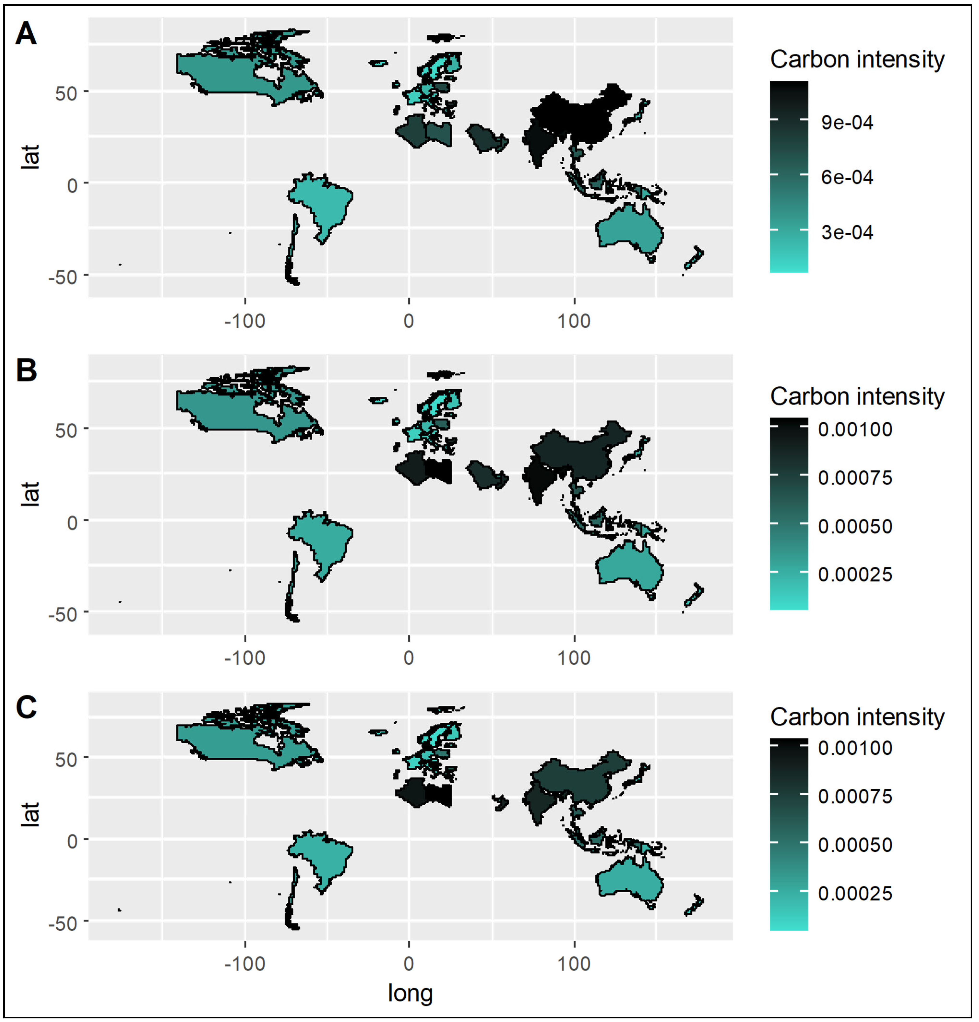
The spatial visualization provides intuitive representation of the uneven but prevailing carbon intensity reductions worldwide from 2010 to 2020, with the steepest declines in nations expanding CCS facilities. This lends further credence to the econometric results pointing to carbon capture deployment as an impactful decarbonisation strategy.

However, the choropleth maps also reveal higher residual carbon intensity in developing countries underscoring the need to accelerate global CCS installations to meet Paris Agreement goals. Expanding access to carbon capture technologies worldwide, especially in the developing world, remains essential for affordable deep decarbonisation by mid-century.

Compared to existing studies, our research offers several scientific advancements. Prior work has largely focused on country-level ordinary least squares (OLS) or two-way fixed-effects approaches within single sectors or limited regional scopes. Ref. [6] conduct life-cycle cost assessments and cascading cost modelling for industrial CCS retrofits in China, while [7] combine process-engineering simulations with panel OLS regressions to evaluate energy-penalty reductions in power-plant CCS. Ref. [8] apply scenario-based pathway modelling to explore CCS scale-up under differing policy regimes, and [9] utilize real-options analysis to value CCS investments under price uncertainty. However, none directly regress multi-sector CCS facility counts on national CI elasticities or account simultaneously for cross-sectional dependence, slope heterogeneity, temporal dynamics, and policy-era effects. Our large-sample DCCE log–log framework addresses these gaps by combining panel-wide common factors, heterogeneous slopes, and lagged dependent variables, thereby producing more robust and policy-relevant elasticity estimates across five CCS applications. This methodological innovation extends the frontiers of CCS empirical research by offering broader research coverage, higher data accuracy, and enhanced interpretability of sectoral decarbonisation potential.

Policy implications arise from our sectoral and regional insights. Developed economies demonstrate high responsiveness to CCS deployment in power, cement, and natural gas processing sectors, suggesting that targeted incentives and infrastructure investments in these areas can yield outsized CI reductions. For emerging economies, modest elasticities point to unrealized potential that could be unlocked through concessional financing, technology transfer partnerships, and regulatory frameworks that de-risk investments. International climate finance mechanisms and multilateral consortia should prioritize capacity building and risk-sharing instruments to accelerate CCS uptake in the Global South. Furthermore, the observed persistence of negative elasticities across pre- and post-2015 policy eras indicates that stable, long-term decarbonisation signals—such as predictable carbon markets or multi-decade decarbonisation roadmaps—can support sustained CCS investments.

Despite our positive findings on CCS deployment, scaling this technology in low-income and developing countries faces significant barriers. High upfront capital costs for capture units and CO₂ transport infrastructure exceed typical public and private financing capacities in these regions [47]. Technological barriers—such as limited local expertise, supply-chain gaps for specialized materials, and the complexity of solvent regeneration—hinder effective project installation and ongoing operation [48]. Infrastructure challenges, including the absence of pipeline networks, monitoring systems, and storage site permitting frameworks, further complicate deployment where regulatory and land-use planning are weak [49]. Moreover, the additional energy demand for capture (10–20% penalty) can strain grids already operating at capacity, risking unintended emissions from backup generation [50]. Overcoming these obstacles will require blended finance schemes, targeted capacity-building programs, and integrated infrastructure planning tailored to resource-constrained settings.

5. Conclusions

Our analysis of 43 countries over 2010–2020, using a dynamic common correlated effects (DCCE) estimator, confirms that scaling up carbon capture and storage (CCS) is an effective lever for reducing national carbon intensity (CI). In high-income panels, a 1% increase in power-and-heat CCS facilities corresponds to a 0.092% drop in CI, and a similar increase in cement-sector CCS yields a 0.132% reduction. By contrast, lower-middle-income panels show modest or even positive CI effects for cement CCS (0.065%), reflecting the early stage of technology adoption and infrastructure. These sectoral elasticities remain robust when we split the sample into pre-2015 and post-2015 periods—capturing the influence of the Paris Agreement and SDGs—and when we compare emerging versus developed economy panels, which serve as proxies for Global South and Global North contexts.

We translate these findings into practice via income-tiered approaches. In high-income countries, CCS incentives should emphasize expansion of power-sector and cement-sector retrofits, for example by extending tax credits to cover half of capture capital costs and by co-funding CO₂ transport and storage infrastructure through public–private partnerships. Upper-middle-income nations would benefit from blended finance models that combine concessional loans with private capital, alongside technology-transfer agreements that adapt proven capture modules to local industrial conditions. In lower-middle- and low-income regions, international climate funds should underwrite pilot CCS hubs that aggregate multiple capture sites into shared pipelines and storage reservoirs, thereby achieving economies of scale and driving elasticities toward the negative values observed in wealthier contexts.

Across all contexts, robust monitoring, reporting, and verification (MRV) frameworks are essential to manage environmental risks such as leakage and induced seismicity. Integrating waste-heat recovery and water-efficient solvents can mitigate the 10–20% energy penalty inherent in CCS processes. Equally important is early and ongoing engagement with stakeholders to build trust and secure social licenses.

References

1. Kongkuah, M. Impact of Economic Variables on CO2 Emissions in Belt and Road and OECD Countries. Environ. Monit. Assess. 2023, 195, 835. [Google Scholar] [CrossRef] [PubMed]
2. Kongkuah, M.; Yao, H.; Fongjong, B.B.; Agyemang, A.O. The Role of CO2 Emissions and Economic Growth in Energy Consumption: Empirical Evidence from Belt and Road and OECD Countries. Environ. Sci. Pollut. Res. 2021, 28, 22488–22509. [Google Scholar] [CrossRef] [PubMed]
3. Kongkuah, M.; Yao, H.; Yilanci, V. The Relationship between Energy Consumption, Economic Growth, and CO2 Emissions in China: The Role of Urbanisation and International Trade. Environ. Dev. Sustain. 2022, 24, 4684–4708. [Google Scholar] [CrossRef]
4. Ozgur, O.; Yilanci, V.; Kongkuah, M. Nuclear Energy Consumption and CO2 Emissions in India: Evidence from Fourier ARDL Bounds Test Approach. Nucl. Eng. Technol. 2022, 54, 1657–1663. [Google Scholar] [CrossRef]
5. IPCC. Global Warming of 1.5 °C—An IPCC Special Report on the Impacts of Global Warming of 1.5 °C Above Pre-Industrial Levels and Related Global Greenhouse Gas Emission Pathways, in the Context of Strengthening the Global Response to the Threat of Climate Change; IPCC: Geneva, Switzerland, 2018. [Google Scholar]
6. Subraveti, S.G.; Rodríguez Angel, E.; Ramírez, A.; Roussanaly, S. Is Carbon Capture and Storage (CCS) Really So Expensive? An Analysis of Cascading Costs and CO2 Emissions Reduction of Industrial CCS Implementation on the Construction of a Bridge. Environ. Sci. Technol. 2023, 57, 2595–2601. [Google Scholar] [CrossRef]
7. Zheng, Y.; Gao, L.; He, S.; Jin, H. Reduction Potential of the Energy Penalty for CO2 Capture in CCS. Front. Energy 2023, 17, 390–399. [Google Scholar] [CrossRef]
8. Shen, M.; Kong, F.; Tong, L.; Luo, Y.; Yin, S.; Liu, C.; Zhang, P.; Wang, L.; Chu, P.K.; Ding, Y. Carbon Capture and Storage (CCS): Development Path Based on Carbon Neutrality and Economic Policy. Carbon Neutrality 2022, 1, 37. [Google Scholar] [CrossRef]
9. Zhang, W.; Dai, C.; Luo, X.; Ou, X. Policy Incentives in Carbon Capture Utilization and Storage (CCUS) Investment Based on Real Options Analysis. Clean Technol. Environ. Policy 2021, 23, 1311–1326. [Google Scholar] [CrossRef]
10. Alizadeh, S.M.; Khalili, Y.; Ahmadi, M. Comprehensive Review of Carbon Capture and Storage Integration in Hydrogen Production: Opportunities, Challenges, and Future Perspectives. Energies 2024, 17, 5330. [Google Scholar] [CrossRef]
11. Viebahn, P.; Nitsch, J.; Fischedick, M.; Esken, A.; Schüwer, D.; Supersberger, N.; Zuberbühler, U.; Edenhofer, O. Comparison of Carbon Capture and Storage with Renewable Energy Technologies Regarding Structural, Economic, and Ecological Aspects in Germany. Int. J. Greenh. Gas Control. 2007, 1, 121–133. [Google Scholar] [CrossRef]
12. Hughes, S. NETL’s Cost of Capturing CO2 from Industrial Sources and Industrial Carbon Capture Retrofit Database USEA Webinar; United States Energy Association: Washington, DC, USA, 2023. [Google Scholar]
13. Oakes, M.; Turner, M. Cost and Performance Baseline for Fossil Energy Plants, Volume 5: Natural Gas Electricity Generating Units for Flexible Operation; National Energy Technology Laboratory: Pittsburgh, PA, USA, 2023. [Google Scholar]
14. Global CCS Institute. CCS Policy, Legal and Regulatory Review; Global CCS Institute: Melbourne, Australia, 2024. [Google Scholar]
15. Klaus, H.; Schmitt, K. Uncertainties and Gaps in Research on Carbon Capture and Storage in Louisiana; Center for Progressive Reform: Washington, DC, USA, 2023. [Google Scholar]
16. Zhang, C.; Yang, H.; Zhao, Y.; Ma, L.; Larson, E.D.; Greig, C. Realizing Ambitions: A Framework for Iteratively Assessing and Communicating National Decarbonization Progress. iScience 2022, 25, 103695. [Google Scholar] [CrossRef]
17. Zhu, Z.; Guo, Y.; Jiang, Z.; Chen, X. The Perspective of Long-Term and Short-Term Incentives on the Business Environment, Executive Incentive Contracts, and Enterprise Innovation. Sage Open 2023, 13, 21582440231206960. [Google Scholar] [CrossRef]
18. Sovacool, B.K.; Newell, P.; Carley, S.; Fanzo, J. Equity, Technological Innovation and Sustainable Behaviour in a Low-Carbon Future. Nat. Hum. Behav. 2022, 6, 326–337. [Google Scholar] [CrossRef]
19. Chen, X.; Mao, S.; Lv, S.; Fang, Z. A Study on the Non-Linear Impact of Digital Technology Innovation on Carbon Emissions in the Transportation Industry. Int. J. Environ. Res. Public Health 2022, 19, 12432. [Google Scholar] [CrossRef] [PubMed]
20. Yang, G.; Nie, Y.; Li, H.; Wang, H. Digital Transformation and Low-Carbon Technology Innovation in Manufacturing Firms: The Mediating Role of Dynamic Capabilities. Int. J. Prod. Econ. 2023, 263, 108969. [Google Scholar] [CrossRef]
21. Slichter, D. Essays in Applied Econometrics. Ph.D. Thesis, University of Rochester, Rochester, NY, USA, 2016. [Google Scholar]
22. Pesaran, M.H.; Chudik, A. Aggregation in Large Dynamic Panels. J. Econom. 2014, 178, 273–285. [Google Scholar] [CrossRef]
23. Javorcik, B.S.; Wei, S.-J. Pollution Havens and Foreign Direct Investment: Dirty Secret or Popular Myth? Contrib. Econ. Anal. Policy 2003, 3. Available online: https://www.nber.org/system/files/working_papers/w8465/w8465.pdf (accessed on 2 May 2025). [CrossRef]
24. York, R.; Rosa, E.A.; Dietz, T. Footprints on the Earth: The Environmental Consequences of Modernity. Am. Sociol. Rev. 2003, 68, 279–300. [Google Scholar] [CrossRef]
25. Seto, K.C.; Güneralp, B.; Hutyra, L.R. Global Forecasts of Urban Expansion to 2030 and Direct Impacts on Biodiversity and Carbon Pools. Proc. Natl. Acad. Sci. USA 2012, 109, 16083–16088. [Google Scholar] [CrossRef]
26. Chudik, A.; Pesaran, M.H. Common Correlated Effects Estimation of Heterogeneous Dynamic Panel Data Models with Weakly Exogenous Regressors. J. Econom. 2015, 188, 393–420. [Google Scholar] [CrossRef]
27. Ghazali, A.; Ali, G. Investigation of Key Contributors of CO 2 Emissions in Extended STIRPAT Model for Newly Industrialized Countries: A Dynamic Common Correlated Estimator (DCCE) Approach. Energy Rep. 2019, 5, 242–252. [Google Scholar] [CrossRef]
28. Eberhardt, M.; Presbitero, A.F. Public Debt and Growth: Heterogeneity and Non-Linearity. J. Int. Econ. 2015, 97, 45–58. [Google Scholar] [CrossRef]
29. Kongkuah, M.; Alessa, N. Renewable Energy and Carbon Intensity: Global Evidence from 184 Countries (2000–2020). Energies 2025, 18, 3236. [Google Scholar] [CrossRef]
30. Pesaran, M.H. Estimation and Inference in Heterogeneous Spatial Panels with a Multifactor Error Structure. J. Econom. 2006, 74, 967–1012. [Google Scholar] [CrossRef]
31. Everaert, G.; De Groote, T. Common Correlated Effects Estimation of Dynamic Panels with Cross-Sectional Dependence. Econom. Rev. 2016, 35, 428–463. [Google Scholar] [CrossRef]
32. Ditzen, J. Xtdcce: Estimating Dynamic Common Correlated Effects in Stata. In SEEC Discussion Papers; Spatial Economics and Econometrics Centre, Heriot Watt University: Edinburgh, UK, 2016. [Google Scholar]
33. Thombs, R. A Guide to Analyzing Large N, Large T Panel Data. Socius 2022, 8, 23780231221117645. [Google Scholar] [CrossRef]
34. Ditzen, J. Estimating Dynamic Common-Correlated Effects in Stata. Stata J. 2018, 18, 585–617. [Google Scholar] [CrossRef]
35. Harding, M.; Lamarche, C.; Pesaran, M.H. Common Correlated Effects Estimation of Heterogeneous Dynamic Panel Quantile Regression Models. J. Appl. Econom. 2020, 35, 294–314. [Google Scholar] [CrossRef]
36. Cao, S.; Zhou, Q. Common Correlated Effects Estimation for Dynamic Heterogeneous Panels with Non-Stationary Multi-Factor Error Structures. Econometrics 2022, 10, 29. [Google Scholar] [CrossRef]
37. Milindi, C.B.; Inglesi-Lotz, R. The Role of Green Technology on Carbon Emissions: Does It Differ across Countries’ Income Levels? Appl. Econ. 2022, 54, 3309–3339. [Google Scholar] [CrossRef]
38. Wang, Q.; Wang, L.; Li, R. Does the Energy Transition Alleviate Environmental Degradation? Evidence from the High Income, Upper and Lower Middle Income Economies. Energy Strategy Rev. 2022, 44, 100966. [Google Scholar] [CrossRef]
39. Caetano, R.V.; Marques, A.C. Nonlinear Relationships between Foreign Direct Investment Decisions and Environmental Degradation in High- and Middle-Income Countries. J. Ind. Bus. Econ. 2023, 51, 135–188. [Google Scholar] [CrossRef]
40. Aslam, M.; Ahmad, A.; Ali, F.; Akhtar, A. Nexus Between Industrialization and Greenhouse Gas Emissions: Impacts on Infant Mortality in Lower-Middle-Income Countries. J. Asian Dev. Stud. 2023, 12, 817–831. [Google Scholar] [CrossRef]
41. Bokka, H.K.; Lau, H.C. Decarbonizing Borneo’s Power and Industry Sectors by Carbon Capture and Storage. Geoenergy Sci. Eng. 2023, 226, 125361. [Google Scholar] [CrossRef]
42. Proskuryakova, L. The Contribution of Low-Carbon Energy Technologies to Climate Resilience. Climate 2023, 11, 231. [Google Scholar] [CrossRef]
43. Hu, J.; Jåstad, E.O.; Bolkesjø, T.F.; Rørstad, P.K. Impact of Large-Scale Bio-CCS Deployment on Forest Biomass Competition and Forest Industry Production. Biomass Bioenergy 2023, 175, 106896. [Google Scholar] [CrossRef]
44. National Energy Technology Laboratory. W.A. Parish Post-Combustion CO2 Capture and Sequestration Demonstration Project; National Energy Technology Laboratory: Washington, DC, USA, 2020. [Google Scholar]
45. Global CCS Institute. CCUS in the Indian Cement Industry: A Review of CO2 Hubs and Storage Facilities. Available online: https://www.globalccsinstitute.com/resources/publications-reports-research/ccus-in-the-indian-cement-industry-a-review-of-co2-hubs-and-storage-facilities/ (accessed on 2 May 2025).
46. Boundary Dam Carbon Capture Project. Available online: https://www.saskpower.com/our-power-future/infrastructure-projects/carbon-capture-and-storage/boundary-dam-carbon-capture-project (accessed on 13 May 2025).
47. Liu, H.; Liang, X. Strategy for Promoting Low-Carbon Technology Transfer to Developing Countries: The Case of CCS. Energy Policy 2011, 39, 3106–3116. [Google Scholar] [CrossRef]
48. Shourideh, M.; Yasseri, S. Uncertainties and Barriers to Carbon Capture and Storage Acceptance & Implementation. Int. J. Coast. Offshore Environ. Eng. (IJCOE) 2023, 8, 18–30. [Google Scholar] [CrossRef]
49. Sajid, M.J.; Zhang, Y.; Janjua, L.R. Breaking Barriers: Assessing Technology Transfer for Climate-Resilient Development. Environ. Technol. Innov. 2024, 33, 103471. [Google Scholar] [CrossRef]
50. IPCC Climate Change 2022: Mitigation of Climate Change (AR6 WG3); Cambridge University Press: Cambridge, UK, 2023.
Figure 1. Increasing trend of global CO2 emissions.
Sustainability 17 06222 g001
Figure 2. Increasing trend of cumulative global CO2 emissions.
Sustainability 17 06222 g002
Figure 3. Spatial distribution of global CO2 emissions in 2020.
Sustainability 17 06222 g003
Figure 4. Spatial distribution of the sampled 43 countries’ carbon intensity: pre and post intervention period.
Sustainability 17 06222 g004
Figure 5. Sampled 43 countries’ carbon intensity ranked: pre and post intervention period.
Sustainability 17 06222 g005