
Analysis of the Synergies of Air Pollutant and Greenhouse Gas Emission Reduction in Typical Chemical Enterprises


Abstract
1. Introduction
2. Research Subjects and Methods
2.1. Subjects of Study and Data Sources
2.2. Methodology
2.2.1. Methods Used to Account for Emissions of Air Pollutants and GHGs
2.2.2. Synergy Analysis Methodology
- (1)
- Synergistic coefficients
- (2)
- Cross-elasticity coefficients based on emissions
- (3)
- Life cycle environmental impact assessment methodology
- (4)
- Cross-elasticity coefficients based on ecological impacts
2.2.3. Scenario Analysis Methodology
3. Results
3.1. Accounting for Air Pollutant and GHG Emissions
3.1.1. Accounting for Air Pollutant Emissions
- (1)
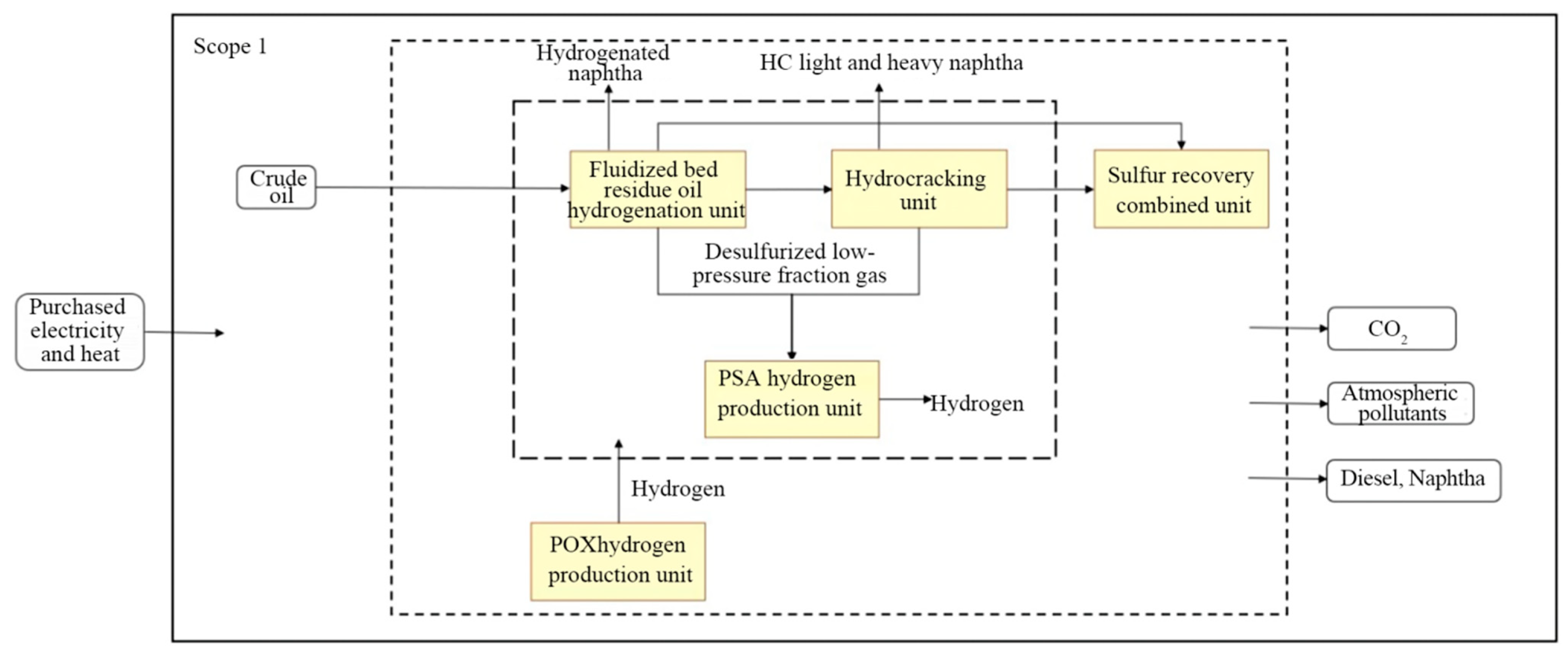
- Refinery Enterprises
- (2)
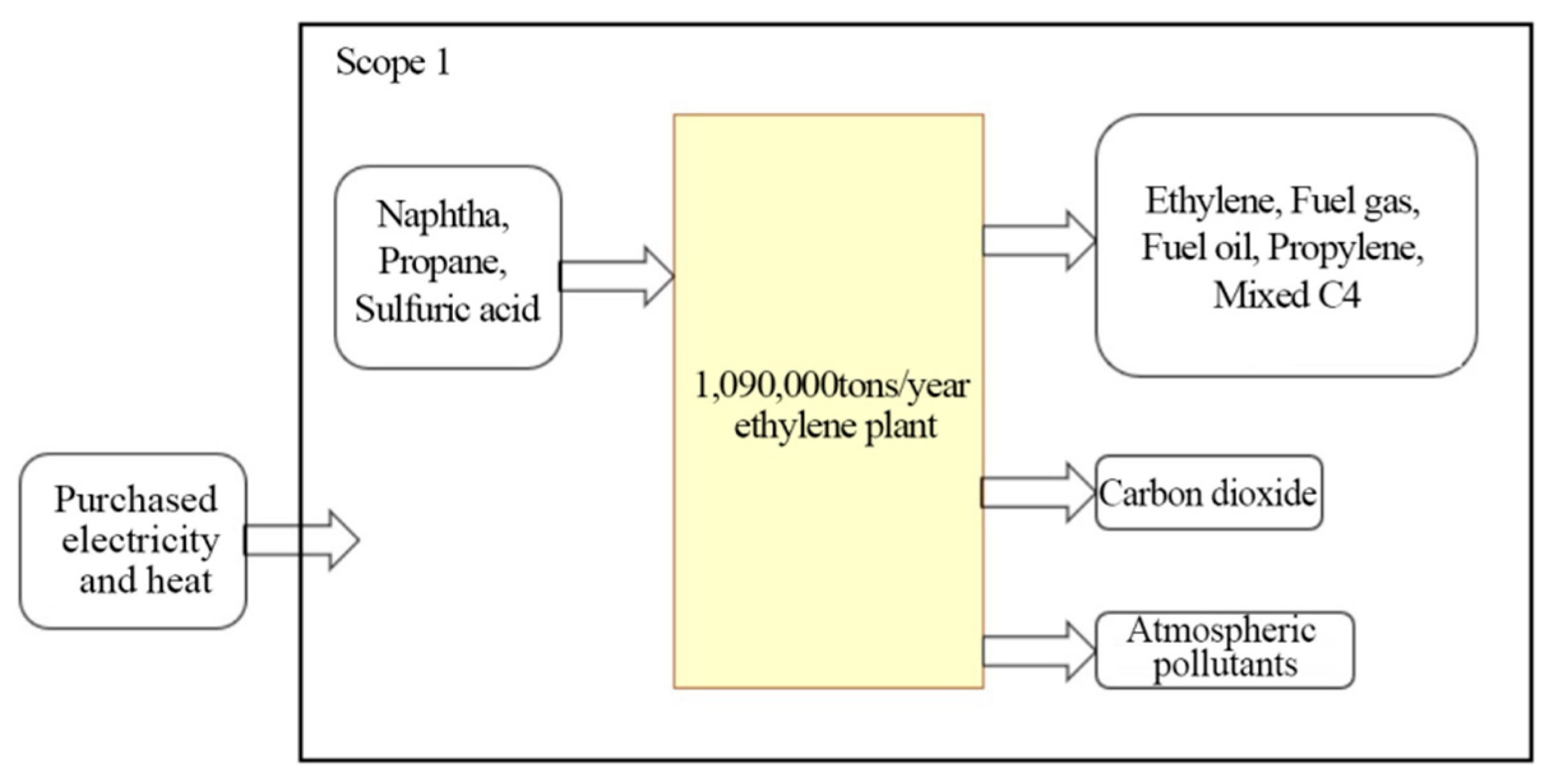
- Ethylene Producers
- (3)
- Chlor-Alkali Producers
3.1.2. Accounting for Carbon Dioxide Emissions
3.2. Air Pollution End-of-Pipe Management Synergies
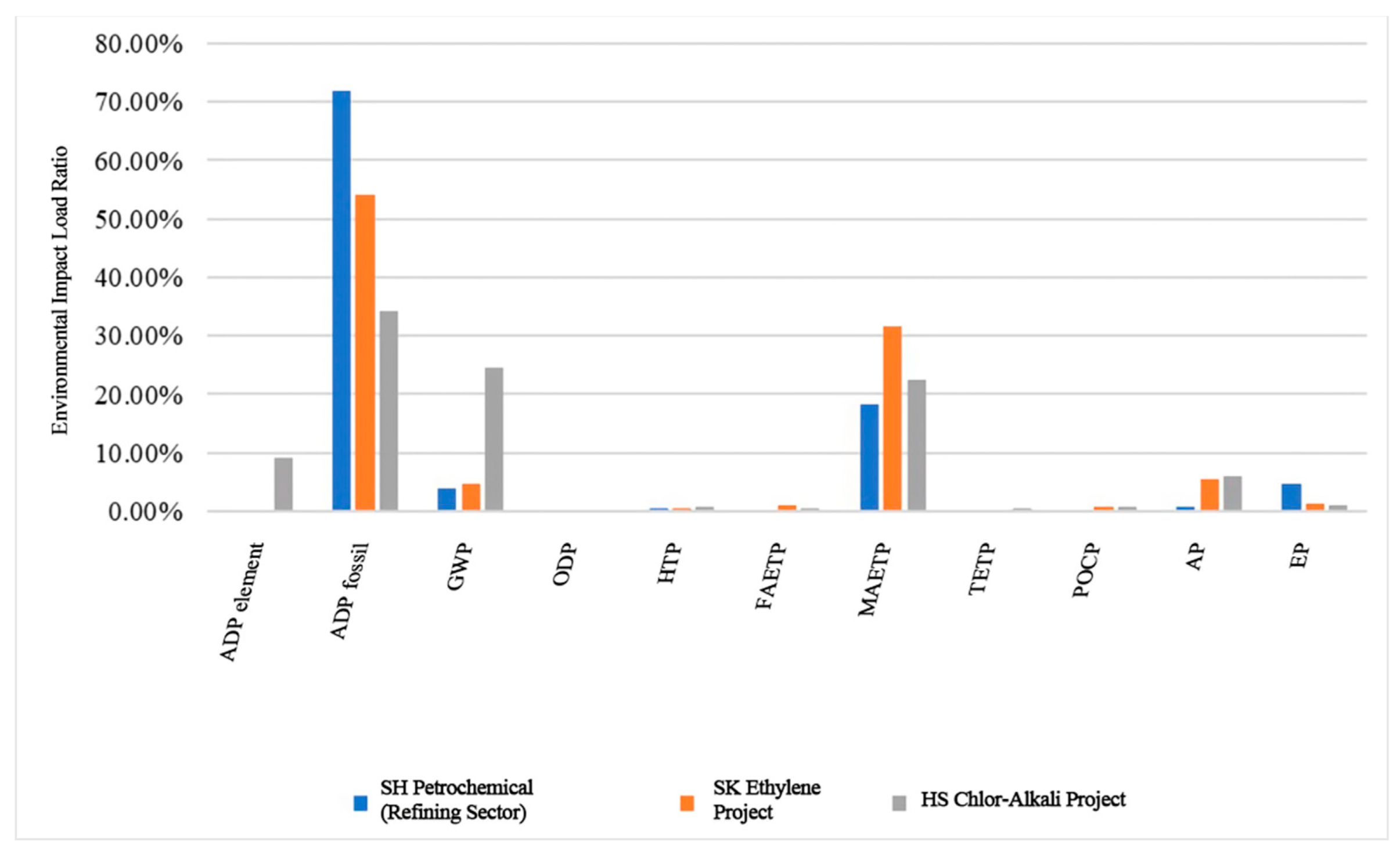
3.3. Life Cycle Environmental Impact Assessment for Typical Products
3.4. Synergistic Effects Based on Impacts on Ecological Environment Under Different Future Scenarios
4. Discussion
5. Conclusions
Author Contributions
Funding
Data Availability Statement
Conflicts of Interest
Appendix A
Appendix B

| Environmental Impact Indicator | Unit | Abbreviation | Standardized Factor |
|---|---|---|---|
| Abiotic depletion | kg Sb eq | ADP element | 1.80 × 10⁻⁸ |
| Abiotic depletion (fossil fuels) | MJ | ADP fossil | 3.18 × 10⁻¹⁴ |
| Global warming (GWP100a) | kg CO2 eq | GWP | 1.99 × 10⁻¹³ |
| Ozone depletion | kg CFC-11 eq | ODP | 1.12 × 10⁻⁸ |
| Human toxicity | kg 1,4-DB eq | HTP | 1.29 × 10⁻¹³ |
| Fresh water aquatic ecotoxicity | kg 1,4-DB eq | FAETP | 1.93 × 10⁻¹² |
| Marine aquatic ecotoxicity | kg 1,4-DB eq | MAETP | 8.57 × 10⁻¹⁵ |
| Terrestrial ecotoxicity | kg 1,4-DB eq | TETP | 2.06 × 10⁻¹¹ |
| Photochemical oxidation | kg C2H4 eq | POCP | 1.18 × 10⁻¹⁰ |
| Acidification | kg SO2 eq | AP | 3.55 × 10⁻¹¹ |
| Eutrophication | kg PO4-eq | EP | 7.58 × 10⁻¹¹ |
| Type | Name | Unit | Refinery Project | Ethylene Project | Chlor-Alkali Project | |||
|---|---|---|---|---|---|---|---|---|
| Baseline Scenario | Low-Carbon Development Scenario | Baseline Scenario | Low-Carbon Development Scenario | Baseline Scenario | Low-Carbon Development Scenario | |||
| Upstream power structure | Thermal power | % | 66.5 | 42.39 | 66.5 | 42.39 | 66.5 | 42.39 |
| Hydroelectricity | % | 15.28 | 18.7 | 15.28 | 18.7 | 15.28 | 18.7 | |
| Nuclear energy | % | 4.72 | 5.65 | 4.72 | 5.65 | 4.72 | 5.65 | |
| Wind power | % | 8.61 | 18.7 | 8.62 | 18.7 | 8.62 | 18.7 | |
| Solar power | % | 4.83 | 14.55 | 4.83 | 14.55 | 4.83 | 14.55 | |
| Process improvement | Substitution of green hydrogen for grey hydrogen | Total energy consumption of electricity and steam decreased by 1.5% | Total energy consumption of electricity and steam decreased by 1.5% | |||||
Appendix C
| Device | Serial Number | Source of Pollution | Governance Measures | Exhaust Volume/ (Nm3/h) | Generation (t/a) | Emissions (t/a) | ||||||
|---|---|---|---|---|---|---|---|---|---|---|---|---|
| SO2 | NOx | Particulate Matter | NMHC | SO2 | NOx | Particulate Matter | NMHC | |||||
| Boiling Bed Residue Hydrogenation Plant | G1-2-1 | Heating furnace flue gas | Low-sulfur fuel gas, ultra-low-NOx burners | 60,000 | 2.02 | 20.16 | 1.01 | 1.01 | 2.02 | 20.16 | 1.01 | 1.01 |
| Hydrocracker | G1-3-1 | Heating furnace flue gas | Low-sulfur fuel gas, ultra-low-NOx burners | 64,500 | 2.17 | 21.67 | 1.08 | 1.08 | 2.17 | 21.67 | 1.08 | 1.08 |
| Sulfur Recovery Combined Unit | G1-6-1 | Incinerator tail gas | RASOC | 62,590 | 600.94 | / | / | / | 13.15 | / | / | / |
| POX Hydrogen Plant | G1-7-1 | Petroleum rubber silo exhaust | Bag filter | 1000 | / | / | 8.40 | 0.17 | / | / | 0.04 | 0.17 |
| G1-7-2 | Slag pond air release | / | 162 | / | / | / | 0.03 | / | / | / | 0.03 | |
| G1-7-3 | Acid gas Stripping tail gas | Washing tower | 13,056 | / | / | / | 54.67 | / | / | / | 11.68 | |
| Total | 605.12 | 41.83 | 10.49 | 56.95 | 17.33 | 41.83 | 2.13 | 13.96 | ||||
| Type | Serial Number | End-of-Pipe Process | SO2 Generation (t/a) | SO2 Emissions (t/a) | NOx Generation (t/a) | NOx Emissions (t/a) | Particulate Matter Generation (t/a) | Particulate Matter Emissions (t/a) | VOC Generation (kg/a) | VOC Emissions (kg/a) |
|---|---|---|---|---|---|---|---|---|---|---|
| Oil boiler | MF0342 | Desulfurization—sodium hydroxide; Denitrification—selective catalytic reduction; Dedusting—Venturi | 129.9 | 0.73 | 369.24 | 71.41 | * | 11.77 | 0 | 0 |
| MF0343 | 135.57 | 0.7 | 313.86 | 72.53 | * | 11.42 | 0 | 0 | ||
| Subtotal | 265.47 | 1.43 | 683.1 | 143.94 | * | 23.19 | 0 | 0 | ||
| Heating crude oil | MF0922 | / | 4.13 | 4.13 | 34.84 | 34.84 | 3.4 | 3.4 | 12,619.98 | 12,619.98 |
| MF0923 | 4.13 | 4.13 | 34.84 | 34.84 | 3.4 | 3.4 | 12,619.98 | 12,619.98 | ||
| MF0924 | 4.13 | 4.13 | 34.84 | 34.84 | 3.4 | 3.4 | 12,619.98 | 12,619.98 | ||
| MF0938 | 6.33 | 6.33 | 53.49 | 53.49 | 5.22 | 5.22 | 19,418.95 | 19,418.95 | ||
| MF0939 | 6.33 | 6.33 | 53.49 | 53.49 | 5.22 | 5.22 | 19,418.95 | 19,418.95 | ||
| Subtotal | 25.05 | 25.05 | 211.5 | 211.5 | 20.64 | 20.64 | 76,697.84 | 76,697.84 | ||
| Total | 290.52 | 26.48 | 894.6 | 355.44 | * | 43.83 | 76,697.84 | 76,697.84 |
| Device | NOx | TSP | SO2 | |||||||||
|---|---|---|---|---|---|---|---|---|---|---|---|---|
| Governance Measures | Generation (t/a) | Emission Reduction (t/a) | Emissions (t/a) | Governance Measures | Generation (t/a) | Emission Reduction (t/a) | Emissions (t/a) | Disposal Measures | Generation (t/a) | Emission Reduction (t/a) | Emissions (t/a) | |
| Ethylene plant | PCC’s patented technology for nitrogen removal | 2386.95 | 834.87 | 1552.08 | Not present | 90.19 | 0 | 90.19 | Not present | 2.26 | 0 | 2.26 |
| Ethylbenzene/styrene (EB/SM) plant | Low-nitrogen burners | 384.66 | 134.63 | 250.03 | Not present | 0 | 0 | 0 | Not present | 5.68 | 0 | 5.68 |
| Polystyrene (PS) units | Low-nitrogen burners | 11.79 | 4.13 | 7.66 | Not present | 0 | 0 | 0 | Not present | 0 | 0 | 0 |
| Acrylonitrile (I and II) plant | AOGI PCC denitrification | 861.66 | 424.34 | 437.32 | Bag filter | 1911.82 | 1902.26 | 9.56 | Not present | 8.82 | 0 | 8.82 |
| Sulfuric acid recovery (SAR) unit | Organic catalytic flue gas desulfurization and denitrification | 139.20 | 37.85 | 101.35 | Not present | 0 | 0 | 0 | Organic catalytic flue gas desulfurization and denitrification | 658.54 | 492.83 | 165.70 |
| Butadiene (BEU1 and 2) plant | Incorporation into acrylonitrile (I and II) unit | Incorporation into acrylonitrile (I and II) unit | Incorporation into acrylonitrile (I and II) unit | |||||||||
| Power center | SCR denitrification | 1125.42 | 776.54 | 348.88 | Ammonia desulfurization and dedusting | 19.13 | 6.31 | 12.82 | Ammonia desulfurization and dedusting | 115.20 | 62.21 | 52.99 |
| Combined heat and power supply | Low-nitrogen burners | 1681.07 | 588.37 | 1092.69 | Not present | 0 | 0 | 0 | Not present | 0 | 0 | 0 |
| Total | / | 4203.80 | 1965.86 | 2237.94 | / | 2021.13 | 1908.57 | 112.56 | / | 790.49 | 555.04 | 235.44 |
| Type | Segment | Disposal Measures | VOCs | ||
|---|---|---|---|---|---|
| Generation (t/a) | Emission Reduction (t/a) | Emissions (t/a) | |||
| Organized emissions | Combustion flue gas emissions | Absorption tower + AOGI thermal incineration | 9187.33 | 9028.53 | 158.80 |
| Organized emissions from processes | Not present | 0.3 | 0 | 0.3 | |
| Flare emissions | Flare thermal incineration | 23,409.68 | 22,941.04 | 468.64 | |
| Subtotal | 32,597.31 | 31,969.57 | 627.74 | ||
| Unorganized emissions | Organic liquid storage and reconciliation of volatilization losses | AOGI thermal incineration | 162.14 | 153 | 9.13 |
| Leakage at static and dynamic sealing points of equipment | Not present | 259.72 | 0.00 | 259.72 | |
| Cooling tower, circulating water, cooling system release | Not present | 358.98 | 0.00 | 358.98 | |
| Subtotal | 780.84 | 153 | 627.83 | ||
| Total | 33,378.15 | 32,122.57 | 1255.57 | ||
| Type | Segment | Device | VOCs | Note | |||
|---|---|---|---|---|---|---|---|
| Disposal Measures | Generation (t/a) | Emission Reduction (t/a) | Emissions (t/a) | ||||
| Unorganized emissions | Organic liquid storage and reconciliation of volatilization losses | Storage tank area | Not present | 156.88 | 0.00 | 156.88 | |
| Leakage at static and dynamic sealing points of equipment | / | Not have | 9.58 | 0.00 | 9.58 | ||
| Organized emissions | Organized emissions from processes | Caustic soda plant | Not present | / | / | / | |
| EDC device | High-temperature incineration | 9.20 | 9.11 | 0.09 | |||
| Hydrogen boiler | Not present | / | / | / | |||
| Combustion flue gas emissions | / | / | / | / | / | Use of hydrogen | |
| Flare emissions | / | / | / | / | / | No flare | |
| Total | 175.66 | 9.11 | 166.55 | ||||
| Type of Fuel | Annual Use | Unit | Calorific Value (GJ/t, GJ/million m3) | Carbon Content Per Unit Calorific Value (tC/GJ) | Carbon Oxidation Rate | CO2 Emissions (tCO2/a) |
|---|---|---|---|---|---|---|
| Fuel oil | 46,386 | t/a | 41.86 | 0.015 | 0.99 | 317,723.08 |
| Petroleum | 183,026.15 | million m3/a | 390 | 0.015 | 0.99 | 3,964,384.78 |
| Total | 4,282,107.86 | |||||
| Type of Fuel | Annual Use | Unit | Calorific Value (GJ/t, GJ/million m(3)) | Carbon Content per Unit Calorific Value (tC/GJ) | Carbon Oxidation Rate | CO2 Emissions (tCO2/a) | Other Information |
|---|---|---|---|---|---|---|---|
| Fuel oil | 95,700 | t/a | 42 | 0.0211 | 0.98 | 304,748.23 | Self-production |
| Fuel gas | 7.9 | Million m3/a | 380 | 0.0153 | 0.99 | 166.73 | Blending of plant-produced hydrogen methane with purchased natural gas, with hydrogen methane components similar to natural gas |
| Total | 304,914.96 | ||||||
| Flare Model | Flare Gas Flow Rate (Million Nm3/a) | Total Carbon Content of Carbon-Containing Compounds (Tons of Carbon/10,000 Nm3) | Carbon Oxidation Rate | CO2 Emissions (tCO2/a) | |
|---|---|---|---|---|---|
| HP-1 | 2639.34 | 6.52 | 0.98 | 61,812.06 | |
| HP-2 | 1376.69 | 9.71 | 0.98 | 48,009.87 | |
| LP-A | 484.04 | 12.50 | 0.98 | 21,736.93 | |
| LP-B | 673.34 | 4.70 | 0.98 | 11,377.80 | |
| LP-C | 2330.20 | 7.85 | 0.98 | 65,768.37 | |
| Low-temperature flare | Inlet pipeline 1 | 0.00 | 13.82 | 0.98 | 0.48 |
| Inlet pipeline 2 | 0.13 | ||||
| Acrylonitrile flare | Craft torch | 7.38 | 10.53 | 0.8 | 318.80 |
| Hydrocyanic acid Norming furnace | 131.40 | ||||
| Total | 209,024.31 | ||||
| Serial Number | Average Tail Gas Flow (Nm3/h) | Annual Cumulative Coking Time (h/a) | Volume Concentration of CO2 in Exhaust Gas (%) | CO2 Emissions (tCO2/a) |
|---|---|---|---|---|
| 1 | 90,100 | 216 | 0.20% | 76.68 |
| 2 | 272,000 | 216 | 0.20% | 231.48 |
| 3 | 272,000 | 216 | 0.20% | 231.48 |
| 4 | 252,000 | 216 | 0.20% | 214.46 |
| 5 | 258,000 | 216 | 0.20% | 219.57 |
| 6 | 276,000 | 216 | 0.20% | 234.89 |
| 7 | 220,000 | 216 | 0.20% | 187.23 |
| 8 | 249,000 | 216 | 0.20% | 211.91 |
| 9 | 240,000 | 216 | 0.20% | 204.25 |
| 10 | 120,000 | 216 | 0.20% | 102.12 |
| 11 | 114,000 | 216 | 0.20% | 97.02 |
| Total | 2011.09 | |||
| Pollutant | Department | End-of-Pipe Management Equipment | Direct CO2 Emissions from End-of-Pipe Treatment (t/a) |
|---|---|---|---|
| VOCs | Vertical fixed roof tanks | AOGI thermal incineration | 480.22 |
| Acrylonitrile I | AOGI thermal incineration | 28,337.55 | |
| Total | 28,817.76 |
| Type of Fuel | Annual Use | Unit | Source | Low-Level Heat Generation (GJ/million Nm3) | Carbon Content per Unit Calorific Value (tC/GJ) | Carbon Oxidation Rate | CO2 Emissions (tCO2/a) |
|---|---|---|---|---|---|---|---|
| Petroleum | 145.2 | million Nm3/a | Natural gas pipeline in chemical zone | 389.31 | 0.0153 | 0.99 | 3139.50 |
| Total | 3139.50 | ||||||
| Device | CO2 Emissions from Raw Material Consumption | CO2 Emissions from Carbonate Use Processes | ||||||||
|---|---|---|---|---|---|---|---|---|---|---|
| Carbon-Containing Raw Materials | Dosage (104t/a) | Carbon-Containing Product | Production (10,000 t/a) | CO2 Emissions (tCO2/a) | Carbonate Type | Consumption (t/a) | CO2 Emission Factor (Tons CO2/Tons Carbonate) | Purity of Carbonate (%) | CO2 Emissions (tCO2/a) | |
| Caustic soda plant | / | 0 | Not present | 0 | 0 | Na2CO3 | 5000 | 0.4149 | 100 | 2074.5 |
| EDC device | Ethylene | 12 | Refined EDC | 41 | 12,698.41 | / | 0 | / | / | 0 |
| Total | 14,772.91 | |||||||||
| Pollutant | Device | Exhaust Port | End-of-Pipe Management Equipment | Direct CO2 Emissions from End-of-Pipe Treatment (t/a) |
|---|---|---|---|---|
| VOCs | EDC device | 1# Incinerator | High-temperature incineration | 138.99 |
| 2# Incinerator | High-temperature incineration | |||
| Total | 138.99 | |||
Appendix D
| Pollutant | Department | Emission Reduction Technologies/ End-of-Pipe Equipment | Equipment Power/ Electricity Consumption Factor | Emission Reduction (t/a) | Electricity Consumption (kWh/a) | Indirect CO2 Emissions (t/a) | Synergistic Coefficient: Amount of Additional CO2 Emitted per Ton of Air Pollutant Reduced (t, both Direct and Indirect) |
|---|---|---|---|---|---|---|---|
| SO2 | Boiling bed residue hydrotreating unit | Low-sulfur fuel gas | / | / | / | / | / |
| Hydrocracker | / | / | / | / | / | ||
| Sulfur recovery combined unit | RASOC renewable wet flue gas | 1280 kW | 587.79 | 10,752,000.00 | 4351.97 | 7.40 | |
| Oil boiler | NaOH | / | 264.04 | / | / | / | |
| NOx | Boiling bed residue hydrotreating unit | Ultra-low-nitrogen burners | / | / | / | / | / |
| Hydrocracker | / | / | / | / | / | ||
| Oil boiler | SCR | 295.5 kW | 539.16 | 2,511,750.00 | 1016.65 | 1.89 | |
| Particulate matter | POX hydrogen plant | Bag filter | 10 kWh/tTSP | 8.36 | 83.58 | 0.03 | 0.0041 |
| Total | 1399.35 | 13,263,833.58 | 5368.66 | 3.84 | |||
| Pollutant | Department | Emission Reduction Technologies/ End-of-Pipe Equipment | Equipment Power/Electricity Consumption Factor | Emission Reduction (t/a) | Electricity Consumption (kWh/a) | Direct CO2 Emissions (t/a) | Indirect CO2 Emissions (t/a) | Synergistic Coefficient: Amount of Additional CO2 Emitted per Ton of Air Pollutant Reduced (t, both Direct and Indirect) |
|---|---|---|---|---|---|---|---|---|
| NOx | Acrylonitrile I | AOGI PCC denitrification | / | 236.38 | / | 0 | / | / |
| Acrylonitrile II | / | 187.97 | / | 0 | / | / | ||
| Power center | SCR denitrification | 295.5 kW | 776.54 | 2,364,000 | 0 | 956.85 | 1.23 | |
| Subtotal | / | / | 776.54 | 2,364,000 | 0 | 956.85 | 1.23 | |
| Particulate matter | Acrylonitrile I | Bag filter | 10 kWh/tTSP | 1628.59 | 16,285.9 | 0 | 6.59 | 0.00405 |
| Acrylonitrile II | 10 kWh/tTSP | 273.66 | 2736.6 | 0 | 1.11 | 0.00405 | ||
| Subtotal | / | / | 1902.25 | 19,022.5 | 0 | 7.70 | 0.00405 | |
| VOCs | Vertical fixed roof tanks | AOGI thermal incineration | 1538.32 kWh/t (VOC) | 100.27 | 154,247.35 | 480.22 | 62.43 | 3.76 |
| Floating roof tanks | 52.73 | 81,115.61 | 32.83 | |||||
| Acrylonitrile I | 4876.14 | 7,501,058.64 | 28,337.55 | 3036.12 | 3.76 | |||
| Acrylonitrile II | 4114.13 | 6,328,841.37 | 2561.66 | |||||
| Power center | 36.03 | 55,425.92 | 22.43 | |||||
| Ground flare | Flare thermal incineration | 611.41 kW | 22,938.15 | 4,891,307.57 | 209,024.31 | 1979.80 | 9.20 | |
| Low-temperature flare | 0.91 | 1395.99 | 0.57 | |||||
| Acrylonitrile flare | 1.98 | 3027.78 | 1.23 | |||||
| Subtotal | / | / | 32,120.33 | 19,016,420.23 | 237,842.08 | 7697.07 | 7.64 | |
| SO2, particulate matter | Power center | Ammonia desulfurization and dust removal | 1124.3 kW | 62.21 t SO2; 6.31 t TSP | 8,994,400 | 0 | 3640.56 | 53.13 |
| SO2, NOx | Sulfuric acid recovery | Organocatalytic flue gas desulfurization | 697.32 kW | 492.83 t SO2; 37.85 t NOx | 5,578,560 | 0 | 2257.97 | 4.25 |
| Total | 35,398.32 | 35,972,402.73 | 237,842.08 | 14,560.15 | 7.13 | |||
| Pollutant | Device | Exhaust Port | End-of-pipe Management Equipment | Equipment Power/ Electricity Consumption Factor | Emission Reduction (t/a) | Electricity Consumption (kWh/a) | Direct CO2 Emissions (t/a) | Indirect CO2 Emissions (t/a) | Synergistic Coefficient: Amount of Additional CO2 Emitted per Ton of Air Pollutant Reduced (t, both Direct and Indirect) |
|---|---|---|---|---|---|---|---|---|---|
| Cl2 | Caustic soda plant | 1# Waste chlorine absorption tower | Alkali absorption | 66,458.98 kWh/(ton Cl2) | 8.73 | 711,111.11 | 0 | 287.83 | 26.90 |
| 2# Waste chlorine absorption tower | 0.67 | ||||||||
| 3# Waste chlorine absorption tower | 1.30 | ||||||||
| Subtotal | 10.70 | 711,111.11 | 0.00 | 287.83 | |||||
| HCl | Caustic soda plant | 1# Hydrochloric acid tail gas treatment (A furnace) | Falling film absorption + water jet | 1,052,380.95 kWh/(ton HCl) | 0.20 | 2,103,634.59 | 0 | 851.47 | 425.95 |
| 1# Hydrochloric acid tail gas treatment (B furnace) | 0.00 | ||||||||
| 1# Hydrochloric acid tail gas treatment (C furnace) | 0.00 | ||||||||
| 1# Hydrochloric acid tail gas treatment (D furnace) | 0.11 | ||||||||
| 1# Hydrochloric acid tail gas treatment (E furnace) | 0.24 | ||||||||
| 1# Hydrochloric acid tail gas treatment (F furnace) | 1.44 | ||||||||
| Subtotal | 2.00 | 2,103,634.59 | 0.00 | 851.47 | |||||
| VOCs | EDC device | 1# Incinerator | High-temperature incineration | 136,915.60 kWh/(tonVOCs) | 4.56 | 1,247,287.57 | 138.99 | 504.85 | 70.67 |
| 2# Incinerator | 4.56 | ||||||||
| Subtotal | 9.11 | 1,247,287.57 | 138.99 | 504.85 | |||||
| Total | 21.81 | 4,062,033.27 | 138.99 | 1644.15 | 81.76 | ||||
Appendix E
| Environmental Impact Indicator | Unit | Abbreviation | Standardized Factor | Standardized Environmental Load Value | Percentage of Environmental Load |
|---|---|---|---|---|---|
| Abiotic depletion | ADP element | kg Sb eq | 7.28 × 10⁻⁵ | 1.31 × 10⁻¹² | 0.02% |
| Abiotic depletion (fossil fuels) | ADP fossil | MJ | 118,867.92 | 3.78 × 10⁻⁹ | 69.48% |
| Global warming (GWP100a) | GWP | kg CO2 eq | 1035.18 | 1.71 × 10⁻¹⁰ | 3.79% |
| Ozone depletion | ODP | kg CFC-11 eq | 3.60 × 10⁻⁵ | 4.07 × 10⁻¹³ | 0.01% |
| Human toxicity | HTP | kg 1,4-DB eq | 182.95 | 2.32 × 10⁻¹¹ | 0.43% |
| Fresh water aquatic ecotoxicity | FAETP | kg 1,4-DB eq | 1.58 | 2.97 × 10⁻¹² | 0.06% |
| Marine aquatic ecotoxicity | MAETP | kg 1,4-DB eq | 1.31 × 10⁵ | 9.89 × 10⁻¹⁰ | 20.59% |
| Terrestrial ecotoxicity | TETP | kg 1,4-DB eq | 0.16 | 2.97 × 10⁻¹² | 0.06% |
| Photochemical oxidation | POCP | kg C2H4 eq | 1.04 × 10⁻¹ | 1.20 × 10⁻¹¹ | 0.23% |
| Acidification | AP | kg SO2 eq | 1.20 | 3.89 × 10⁻¹¹ | 0.78% |
| Eutrophication | EP | kg PO4- eq | 3.27 | 2.47 × 10⁻¹⁰ | 4.56% |
| Abiotic depletion | / | / | / | 5.44 × 10⁻⁹ | 100.00% |
| Environmental Impact Indicator | Unit | Abbreviation | Standardized Factor | Standardized Environmental Load Value | Percentage of Environmental Load |
|---|---|---|---|---|---|
| Abiotic depletion | ADP element | kg Sb eq | 3.05 × 10⁻⁴ | 3.60 × 10⁻¹² | 0.05% |
| Abiotic depletion (fossil fuels) | ADP fossil | MJ | 1.19 × 10⁵ | 3.80 × 10⁻⁹ | 53.94% |
| Global warming (GWP100a) | GWP | kg CO2 eq | 1.83 × 10³ | 3.63 × 10⁻¹⁰ | 5.15% |
| Ozone depletion | ODP | kg CFC-11 eq | 1.53 × 10⁻³ | 1.71 × 10⁻¹¹ | 0.24% |
| Human toxicity | HTP | kg 1,4-DB eq | 261 | 3.37 × 10⁻¹¹ | 0.48% |
| Fresh water aquatic ecotoxicity | FAETP | kg 1,4-DB eq | 39.5 | 7.63 × 10⁻¹¹ | 1.08% |
| Marine aquatic ecotoxicity | MAETP | kg 1,4-DB eq | 2.58 × 10⁵ | 2.21 × 10⁻⁹ | 31.37% |
| Terrestrial ecotoxicity | TETP | kg 1,4-DB eq | 0.921 | 1.90 × 10⁻¹¹ | 0.27% |
| Photochemical oxidation | POCP | kg C2H4 eq | 0.438 | 5.17 × 10⁻¹¹ | 0.73% |
| Acidification | AP | kg SO2 eq | 10.6 | 3.77 × 10⁻¹⁰ | 5.35% |
| Eutrophication | EP | kg PO4- eq | 1.24 | 9.40 × 10⁻¹¹ | 1.33% |
| Abiotic depletion | / | / | / | 7.05 × 10⁻⁹ | 100.00% |
| Environmental Impact Indicator | Unit | Abbreviation | Standardized Factor | Standardized Environmental Load Value | Percentage of Environmental Load |
|---|---|---|---|---|---|
| Abiotic depletion | ADP element | kg Sb eq | 0.00504 | 5.95 × 10⁻¹¹ | 9.22% |
| Abiotic depletion (fossil fuels) | ADP fossil | MJ | 6.94 × 10³ | 2.21 × 10⁻¹⁰ | 34.23% |
| Global warming (GWP100a) | GWP | kg CO2 eq | 805 | 1.60 × 10⁻¹⁰ | 24.78% |
| Ozone depletion | ODP | kg CFC-11 eq | 9.72 × 10⁻⁶ | 1.09 × 10⁻¹³ | 0.02% |
| Human toxicity | HTP | kg 1,4-DB eq | 41.2 | 5.32 × 10⁻¹² | 0.82% |
| Fresh water aquatic ecotoxicity | FAETP | kg 1,4-DB eq | 1.21 | 2.34 × 10⁻¹² | 0.36% |
| Marine aquatic ecotoxicity | MAETP | kg 1,4-DB eq | 1.68 × 10⁴ | 1.44 × 10⁻¹⁰ | 22.31% |
| Terrestrial ecotoxicity | TETP | kg 1,4-DB eq | 1.47 × 10⁻¹ | 3.03 × 10⁻¹² | 0.47% |
| Photochemical oxidation | POCP | kg C2H4 eq | 4.70 × 10⁻² | 5.55 × 10⁻¹² | 0.86% |
| Acidification | AP | kg SO2 eq | 1.08 | 3.83 × 10⁻¹¹ | 5.93% |
| Eutrophication | EP | kg PO4- eq | 8.47 × 10⁻² | 6.42 × 10⁻¹² | 0.99% |
| Abiotic depletion | / | / | / | 6.46 × 10⁻¹⁰ | 100.00% |
Appendix F
| Abbreviation | Full Name |
|---|---|
| AOGI | Acrylonitrile Gas Incineration |
| GHG | Greenhouse Gas |
| CGE | Computable General Equilibrium |
| IES | Integrated Environmental Strategies |
| IIASA | International Institute for Applied Systems Analysis |
| LCA | Life Cycle Assessment |
| RASOC | Regenerable Absorption Process for SOx Cleanup |
| NMHC | Non-Methane Total Hydrocarbons |
| FGD | Flue Gas Desulfurization |
| SCR | Selective Catalytic Reduction |
References
- Arrow, K.J. Global Climate Change: A Challenge to Policy. Econ. Voice 2007, 4, 2. [Google Scholar] [CrossRef]
- Zhao, Q. A Review of Pathways to Carbon Neutrality from Renewable Energy and Carbon Capture. E3S Web Conf. 2021, 245, 01018. [Google Scholar] [CrossRef]
- Pang, L.; Wen, H.; Chang, J.; Li, Y.; Cai, B.; Lei, Y.; Yan, G.; Lv, C.; Zhang, L.; Qi, Z.; et al. Pathway of Carbon Emission Peak for China’s Petrochemical and Chemical Industries. Res. Environ. Sci. 2022, 35, 356–367. [Google Scholar] [CrossRef]
- Chen, F. Air Pollution Control Strategy of Petrochemical Enterprises. Chem. Eng. Des. Commun. 2020, 46, 199–212. [Google Scholar] [CrossRef]
- Wang, Y.; Li, B.; Zhang, Y.; Zhao, Y.; Miao, C.; An, J. Spatiotemporal Characteristics and Influencing Factors of the Synergistic Effect of Pollution Reduction and Carbon Reduction in China. Environ. Sci. 2024, 45, 4993–5002. [Google Scholar] [CrossRef]
- Liu, Z.; Tang, Y.; Zhao, J.; Zhang, X.; Lu, G. Analysis and suggestions of the synergy management and development of air quality pollutant emission inventory and greenhouse gas emission inventory—Helping synergize the reduction of pollution and carbon emissions. Environ. Prot. Sci. 2024, 50, 49–53. [Google Scholar] [CrossRef]
- Bollen, J.; Brink, C. Air pollution policy in Europe: Quantifying the interaction with greenhouse gases and climate change policies. Energy Econ. 2014, 46, 202–215. [Google Scholar] [CrossRef]
- Brendemoen, A.; Vennemo, H. A Climate Treaty and the Norwegian Economy: ACGE Assessment. Energy J. 1994, 15, 77–93. [Google Scholar]
- Mardones, C.; Ortega, J. The individual and combined impact of environmental taxes in Chile− A flexible computable general equilibrium analysis. J. Environ. Manag. 2023, 325, 116508. [Google Scholar] [CrossRef]
- West, J.J.; Osnaya, P.; Laguna, I.; Martínez, J.; Fernández, A. Co-control of urban air pollutants and greenhouse gases in Mexico City. Environ. Sci. Technol. 2004, 38, 3474–3481. [Google Scholar] [CrossRef]
- Pu, Y. Research on the Emission Characteristics and Cost Prediction of Air Pollutants for China’s Thermal Power Generation: A GAINS-China Model-Based Spatial Analysis. Master’s Thesis, Jilin University, Changchun, China, 2020. [Google Scholar]
- Wagner, F.; Amann, M.; Borken-Kleefeld, J.; Cofala, J.; Höglund-Isaksson, L.; Purohit, P.; Rafaj, P.; Schöpp, W.; Winiwarter, W. Sectoral marginal abatement cost curves: Implications for mitigation pledges and air pollution co-benefits for Annex I countries. Sustain. Sci. 2012, 7, 169–184. [Google Scholar] [CrossRef]
- Liu, D.; Li, X.; Wang, D.; Wu, H.; Li, Y.; Li, Y.; Qiao, Q.; Yin, Z. An evaluation method for synergistic effect of air pollutants and CO2 emission reduction in the Chinese petroleum refining technology. J. Environ. Manag. 2024, 371, 123169. [Google Scholar] [CrossRef]
- Chan, Y.; Tang, H.; Li, X.; Ma, W.; Tang, W. Correction: Chan et al. Analysis of the Synergies of Cutting Air Pollutants and Greenhouse Gas Emissions in an Integrated Iron and Steel Enterprise in China. Sustainability 2023, 15, 13231. Sustainability 2025, 17, 2900. [Google Scholar] [CrossRef]
- Cai, J.; Gao, S.; Sun, X.; Jiang, P.; Zhen, J.; Zhang, M. Synthesis of research on synergies between environmental, economic and social development. China Popul. Resour. Environ. 2016, S2, 4. [Google Scholar]
- Gu, A.; Teng, F.; Feng, X. Effects of pollution control measures on carbon emission reduction in China: Evidence from the 11th and 12th Five-Year Plans. Clim. Policy 2018, 18, 198–209. [Google Scholar] [CrossRef]
- Wang, S.; Lv, L.; Zhang, B.; Wang, S.; Wu, J.; Fu, J.; Luo, H. Multi Objective Programming Model of Low-Cost Path for China’s Peaking Carbon Dioxide Emissions and Carbon Neutrality. Res. Environ. Sci. 2021, 34, 2044–2055. [Google Scholar] [CrossRef]
- Li, J.; Li, H. Decomposition of carbon emission factors and analysis of emission reduction potential of petrochemical industry in Beijing-Tianjin-Hebei under the perspective of industrial transfer. Res. Environ. Sci. 2020, 33, 324–332. [Google Scholar] [CrossRef]
- Yu, S.; Zhang, S.; Zhang, Z.-J.; Qu, Y.-Z.; Liu, T.-S. Scenario modeling and effect assessment of pollution reduction and carbon reduction synergistic control in Beijing. Environ. Sci. 2023, 44, 1998–2008. [Google Scholar] [CrossRef]
- Tang, Y. Research on the Accounting of Synergistic Emission Reduction Effect of Air Pollutants and Greenhouse Gases and Load Optimization Control of Thermal Power Plants. Master’s Thesis, North China Electric Power University, Beijing, China, 2014. [Google Scholar]
- Ministry of Environmental Protection. Calculation Methods for Actual Pollutant Emissions in 17 Industries Including Thermal Power under Emission Permit Management (Including Emission Factors and Material Balance Methods) (Provisional); Ministry of Environmental Protection: Beijing, China, 2017. [Google Scholar]
- Chinese Academy of Environmental Sciences. Guidelines for the Compilation of Provincial Greenhouse Gas Inventories; Chinese Academy of Environmental Sciences: Beijing, China, 2011. [Google Scholar]
- Wang, Y.; Ren, Y. Synergistic Strategies for Carbon Emission Reduction and Atmospheric Environment Management. Low Carbon World 2024, 14, 43–45. [Google Scholar] [CrossRef]
- O’Neill, N.F.; Ma, J.M.; Walther, D.C.; Brockway, L.R.; Ding, C.; Lin, J. A modified total equivalent warming impact analysis: Addressing direct and indirect emissions due to corrosion. Sci. Total Environ. 2020, 741, 140312. [Google Scholar] [CrossRef]
- Liu, T.; Bian, X.; Wu, S.; Liang, S.; Xu, Q.; Wei, X. Overview and outlook of carbon emission accounting for power systems. Power Syst. Prot. Control 2024, 52, 176–187. [Google Scholar] [CrossRef]
- Tang, H. Accounting for Greenhouse Gas Emissions in Iron and Steel Enterprises and Analyzing the Synergistic Effect of Air Pollutant Emission Reduction and Greenhouse Gas Emission; Fudan University: Shanghai, China, 2021. [Google Scholar]
- Liu, K.; Li, X.; Liu, T.; Li, B.; Dai, Y.; Meng, C.; Hao, Y. Example analysis of evaluation of synergistic control effect of pollution reduction and carbon reduction in iron and steel enterprises’ technological reform projects. Environ. Eng. 2022, 780–783. [Google Scholar] [CrossRef]
- Mao, X.; Zeng, A.; Liu, S.; Hu, T.; Xing, Y. Evaluation of synergistic control effects of sulfur, nitrogen and carbon in iron and steel industry. J. Environ. Sci. 2012, 32, 1253–1260. [Google Scholar] [CrossRef]
- Zhai, Y.; Zhang, T.; Shen, X.; Ma, X.; Hong, J. Development of life cycle assessment method. Resour. Sci. 2021, 43, 446–455. [Google Scholar]
- ISO 14040:2006; Environmental Management—Life Cycle Assessment—Principles and Framework. ISO: Geneva, Switzerland, 2006.
- Petrescu, L.; Chisalita, D.-A.; Cormos, C.-C.; Manzolini, G.; Cobden, P.; van Dijk, H.A.J. Life Cycle Assessment of SEWGS Technology Applied to Integrated Steel Plants. Sustainability 2019, 11, 1825. [Google Scholar] [CrossRef]
- Wang, Q.; Zhang, L.; Cang, D. LCA life cycle evaluation of pelletizing process in iron and steel industry based on GaBi software. Metall. Energy 2017, 36, 3–6+32. [Google Scholar]
- Shi, W. Life Cycle Assessment of Different Flue Gas Desulfurization Processes in Coal-Fired Power Plants. Master’s Thesis, Shandong University, Jinan, China, 2016. [Google Scholar]
- Dreyer, L.C.; Niemann, A.L.; Hauschild, M.Z. Comparison of Three Different LCIA Methods: EDIP97, CML2001 and Eco-indicator 99: Does it matter which one you choose? Int. J. Life Cycle Assess. 2003, 8, 191–200. [Google Scholar] [CrossRef]
- International Iron and Steel Institute. World Steel Life Cycle Inventory Methodology Report. 2000. Available online: https://worldsteel.org/zhhans/publications/bookshop/life-cycle-inventory-report-2018/ (accessed on 16 May 2025).
- Duan, L.; Li, Z.; Pu, X. Scenario modeling of air quality improvement in Chengdu-Chongqing area in the medium and long term: A comprehensive strategy for pollution reduction and carbon reduction. China Environ. Sci. 2024, 44, 1756–1768. [Google Scholar] [CrossRef]
- Zhao, C.; Yuan, P.; Bian, W.; Tong, G.; Niu, Q. Application and Development of Green and Low-Carbon Technologies in Chlor-alkali Chemical Industry. China Chlor-Alkali 2023, 11, 54–57. [Google Scholar]
- Sun, J.; Kong, Y.; Chen, Y.; Xiang, T.; Gao, B.; Luo, S. A Review of Whole Chain Carbon Emission Accounting Methods for Power Systems. Autom. Electr. Power Syst. 2024, accepted. [Google Scholar]
- Liu, S.; Deng, C. Key Points of Strong Accounting of Pollutant Sources in Environmental Impact Assessment. Leather Manuf. Environ. Technol. 2022, 3, 192–194. [Google Scholar] [CrossRef]
- Zhang, L.; Fan, N.; Guo, S. Problems and Suggestions of Carbon Emission Assessment and Accounting in China’s Chemical Industry. Environ. Prot. Oil Gas Fields 2023, 33, 5–11. [Google Scholar] [CrossRef]
- Liang, S. Improvement of VOCs Emission Inventory for Anthropogenic Sources in China and Its Characterization. Ph.D. Thesis, South China University of Technology, Guangzhou, China, 2022. [Google Scholar] [CrossRef]
- Shanghai Environmental Protection Bureau. Calculation Method for Volatile Organic Compound Emissions in the Petrochemical Industry in Shanghai (Revised in 2017); Shanghai Environmental Protection Bureau: Shanghai, China, 2017. [Google Scholar]
- Shanghai Ecological and Environmental Bureau. Shanghai Guidelines for Greenhouse Gas Emission Accounting and Reporting (Provisional); Shanghai Ecological and Environmental Bureau: Shanghai, China, 2022. [Google Scholar]


| Enterprise | Category | Source of Pollution | Pollutant | Accounting Method |
|---|---|---|---|---|
| SH Petrochemical (refining segment) | Organized emissions | Process-heating furnaces | SO2 | Material balance algorithm |
| NOx, particulate matter, NMHC | Analogy | |||
| Sulfur recovery unit off-gas | SO2 | Field measurement | ||
| Other organized emissions | SO2 | Material balance algorithm | ||
| NOx, particulate matter | Analogy | |||
| VOCs | Field measurement | |||
| Unorganized emissions | Equipment and piping dynamic and static sealing points | VOCs | Equation method | |
| SK Ethylene | Organized emissions | Combustion flue gas emissions | VOCs | Field measurement |
| Organized emissions from processes | VOCs | Field measurement | ||
| Flare emissions | VOCs | Material balance algorithm | ||
| Other organized emissions | SO2, NOx, particulate matter | Field measurement | ||
| Unorganized emissions | Volatile losses in the storage and blending of organic liquids | VOCs | TANKS model | |
| Equipment static and dynamic sealing leakage | VOCs | Equation method + coefficient method | ||
| Cooling tower, circulating water cooling system release | VOCs | Equation method | ||
| HS Chlor-Alkali | Organized emissions | Organized emissions from processes | Cl2, HCl, VOCs | Field measurement |
| Unorganized emissions | Volatile losses in the storage and blending of organic liquids | VOCs | TANKS model | |
| Equipment static and dynamic sealing leakage | VOCs | Equation method |
| Pollutant | SO2 | NOx | Particulate Matter | NMHC | VOCs |
|---|---|---|---|---|---|
| Process emissions | 17.33 | 41.83 | 2.13 | 13.96 | / |
| Combustion process emissions | 26.48 | 355.44 | 43.83 | / | 76.70 |
| Total | 43.81 | 397.27 | 45.96 | 13.96 | 76.70 |
| Device | Sealing Points (pcs) | VOC Emissions /(t/a) | |||||||
|---|---|---|---|---|---|---|---|---|---|
| Connectors | Open-Ended Valves or Open-Ended Lines | Valves | Compressors, Agitators, Pressure Relief Equipment | Pump | Flange | Other | Total | ||
| Boiling bed residue hydrogenation unit | 0 | 0 | 9500 | 6 | 30 | 16,500 | 0 | 26,036 | 50.73 |
| High-pressure hydrocracker | 0 | 0 | 5230 | 238 | 31 | 7401 | 0 | 12,900 | 24.78 |
| POX hydrogen generation unit | 0 | 0 | 3620 | 229 | 54 | 2734 | 0 | 6637 | 12.22 |
| PSA hydrogen generation unit | 0 | 0 | 75 | 1 | 0 | 165 | 0 | 241 | 0.48 |
| Sum | 45,814 | 88.21 | |||||||
| Source of Pollution | NOx | TSP | SO2 | ||||||
|---|---|---|---|---|---|---|---|---|---|
| Generation | Reduction | Emission | Generation | Reduction | Emission | Generation | Reduction | Emission | |
| Process installations | 3784.26 | 1435.82 | 2348.44 | 2002.01 | 1902.26 | 99.75 | 675.3 | 492.83 | 182.46 |
| Power center and cogeneration | 2806.49 | 1364.91 | 1441.57 | 19.13 | 6.31 | 12.82 | 115.20 | 62.21 | 52.99 |
| Total | 4203.80 | 1965.86 | 2237.94 | 2021.13 | 1908.57 | 112.56 | 790.49 | 555.04 | 235.44 |
| Type | VOCs | ||
|---|---|---|---|
| Generation | Reduction | Emission | |
| Organized emissions | 32,597.31 | 31,969.57 | 627.74 |
| Unorganized emissions | 780.84 | 153 | 627.83 |
| Total | 33,378.15 | 32,122.57 | 1255.57 |
| Device | Cl2 | HCl | ||||||
|---|---|---|---|---|---|---|---|---|
| Disposal Measures | Generation | Reduction | Emissions | Disposal Measures | Generation | Reduction | Emission | |
| Caustic soda plant | Alkali absorption | 10.71 | 10.70 | 0.01 | Falling film absorption + water jet | 2.08 | 2.00 | 0.08 |
| Ethylene dichloride (EDC) plant | / | 0.04 | 0.00 | 0.04 | / | 0.03 | 0.00 | 0.03 |
| Hydrogen boiler | / | 0.00 | 0.00 | 0.00 | / | 0.00 | 0.00 | 0.00 |
| Total | 10.75 | 10.70 | 0.05 | 2.11 | 2.00 | 0.11 | ||
| Type | VOCs | ||
|---|---|---|---|
| Generation | Reduction | Emission | |
| Organized emissions | 9.20 | 9.11 | 0.09 |
| Unorganized emissions | 166.46 | 0.00 | 166.46 |
| Total | 175.66 | 9.11 | 166.55 |
| Enterprise | Sources of CO2 Emissions | CO2 Emissions |
|---|---|---|
| SH Petrochemical | CO2 emissions from fuel combustion | 4,282,108 |
| Implied CO2 emissions from net purchases of electricity and heat | 128,148 | |
| Total | 4,410,256 | |
| SK Ethylene | CO2 emissions from fuel combustion | 304,915 |
| CO2 emissions from flare combustion | 209,024 | |
| CO2 emissions from processes | 2011 | |
| Implied CO2 emissions from net purchases of electricity and heat | 485,950 | |
| Direct carbon emissions from end-of-pipe management | 28,818 | |
| Total | 1,030,719 | |
| HS Chlor-Alkali | CO2 emissions from fuel combustion | 3139 |
| CO2 emissions from processes | 14,773 | |
| Implied CO2 emissions from net purchases of electricity and heat | 707,580 | |
| Direct carbon emissions from end-of-pipe management | 139 | |
| Total | 725,631 |
| Pollutant | Source of Emissions | Emission Reduction Technologies/End-of-Pipe Equipment | Synergistic Coefficient: Amount of Additional CO2 Emitted per Ton of Air Pollutant Reduced (t, Both Direct and Indirect) |
|---|---|---|---|
| SO2 | Sulfur recovery combined unit | RASOC renewable wet flue gas | 7.4 |
| NOx | Oil boilers | SCR | 1.9 |
| Particulate matter | POX hydrogen generation plant | Bag filter | 0.004 |
| Pollutant | Source of Emissions | Emission Reduction Technologies/End-of-Pipe Equipment | Synergistic Coefficient: Amount of Additional CO2 Emitted per Ton of Air Pollutant Reduced (t, Both Direct and Indirect) |
|---|---|---|---|
| NOx | Power center | SCR denitrification | 1.2 |
| Particulate matter | Acrylonitrile I, II | Bag filter | 0.004 |
| VOCs | Storage tank, acrylonitrile I and II, power center | AOGI thermal incineration | 3.8 |
| Ground torch, cryogenic torch, acrylonitrile torch | Flare thermal incineration | 9.2 | |
| SO2, particulate matter | Power center | Ammonia desulfurization and dedusting | 53.1 |
| SO2, NOx | Sulfuric acid recovery | Organic catalytic flue gas desulfurization and denitrification | 4.2 |
| Pollutant | Source of Emissions | Emission Reduction Technologies/End-of-Pipe Equipment | Synergistic Coefficient: Amount of Additional CO2 Emitted per Ton of Air Pollutant Reduced (t, Both Direct and Indirect) |
|---|---|---|---|
| Cl2 | Caustic soda unit | Alkali absorption | 26.9 |
| HCl | Caustic soda unit | Falling film absorption + water jet | 425.9 |
| VOCs | EDC unit | High-temperature incineration | 70.7 |
| Enterprise | Pollutant | Emission Reduction Measures/Technologies | Air Pollutant Emission Reduction (t) | Direct Synergistic CO2 Emissions (t) | Indirect Synergistic CO2 Emissions (t) | Cross-Elasticity Coefficient |
|---|---|---|---|---|---|---|
| SH Petrochemical | SO2 | RASOC renewable wet flue gas | 587.8 | / | 4352.0 | −0.001 |
| NOx | SCR | 539.2 | / | 1016.6 | −0.0004 | |
| SK Ethylene | NOx | SCR | 776.5 | 0 | 956.8 | −0.001 |
| Particulate matter | Bag filter | 1902.2 | 0 | 7.70 | −7.5 × 10⁻⁶ | |
| VOCs | AOGI thermal incineration | 9179.3 | 28,817.8 | 5715.5 | −0.03 | |
| Flare thermal incineration | 22,941.0 | 209,024.3 | 1981.6 | −0.2 | ||
| SO2, TSP | Ammonia desulfurization and dedusting | 68.5 | 0 | 3640.6 | −0.007 | |
| SO2, NOx | Organic catalytic flue gas desulfurization and denitrification | 530.7 | 0 | 2258.0 | −0.003 | |
| HS Chlor-Alkali | Cl2 | Alkali absorption | 10.7 | / | 287.8 | −0.0004 |
| HCl | Falling film absorption + water jet | 2.0 | / | 851.5 | −0.001 | |
| VOCs | High-temperature incineration | 9.1 | 139.0 | 504.8 | −0.002 |
| Sector | Scenario Comparison | Type of Indicator | Value |
|---|---|---|---|
| Refining industry | Low-carbon development scenario vs. baseline scenario | ΔEIAP | −5.5% |
| ΔEIGHG | −17% | ||
| Ethylene industry | Low-carbon development scenario vs. baseline scenario | ΔEIAP | −2.1% |
| ΔEIGHG | −8.8% | ||
| Chlor-alkali industry | Low-carbon development scenario vs. baseline scenario | ΔEIAP | −0.29% |
| ΔEIGHG | −15.0% |
| Sector | Scenario | SEA/C |
|---|---|---|
| Refining industry | Low-carbon development scenario | 0.32 |
| Ethylene industry | Low-carbon development scenario | 0.24 |
| Chlor-alkali industry | Low-carbon development scenario | 0.019 |
Disclaimer/Publisher’s Note: The statements, opinions and data contained in all publications are solely those of the individual author(s) and contributor(s) and not of MDPI and/or the editor(s). MDPI and/or the editor(s) disclaim responsibility for any injury to people or property resulting from any ideas, methods, instructions or products referred to in the content. |
© 2025 by the authors. Licensee MDPI, Basel, Switzerland. This article is an open access article distributed under the terms and conditions of the Creative Commons Attribution (CC BY) license (https://creativecommons.org/licenses/by/4.0/).
Share and Cite
Gong, Q.; Chan, Y.; Xia, Y.; Tang, W.; Ma, W. Analysis of the Synergies of Air Pollutant and Greenhouse Gas Emission Reduction in Typical Chemical Enterprises. Sustainability 2025, 17, 6263. https://doi.org/10.3390/su17146263
Gong Q, Chan Y, Xia Y, Tang W, Ma W. Analysis of the Synergies of Air Pollutant and Greenhouse Gas Emission Reduction in Typical Chemical Enterprises. Sustainability. 2025; 17(14):6263. https://doi.org/10.3390/su17146263
Chicago/Turabian StyleGong, Qi, Yatfei Chan, Yijia Xia, Weiqi Tang, and Weichun Ma. 2025. "Analysis of the Synergies of Air Pollutant and Greenhouse Gas Emission Reduction in Typical Chemical Enterprises" Sustainability 17, no. 14: 6263. https://doi.org/10.3390/su17146263
APA StyleGong, Q., Chan, Y., Xia, Y., Tang, W., & Ma, W. (2025). Analysis of the Synergies of Air Pollutant and Greenhouse Gas Emission Reduction in Typical Chemical Enterprises. Sustainability, 17(14), 6263. https://doi.org/10.3390/su17146263