

Master Production Scheduling with Consideration of Utilization-Dependent Exhaustion and Capacity Load


Abstract
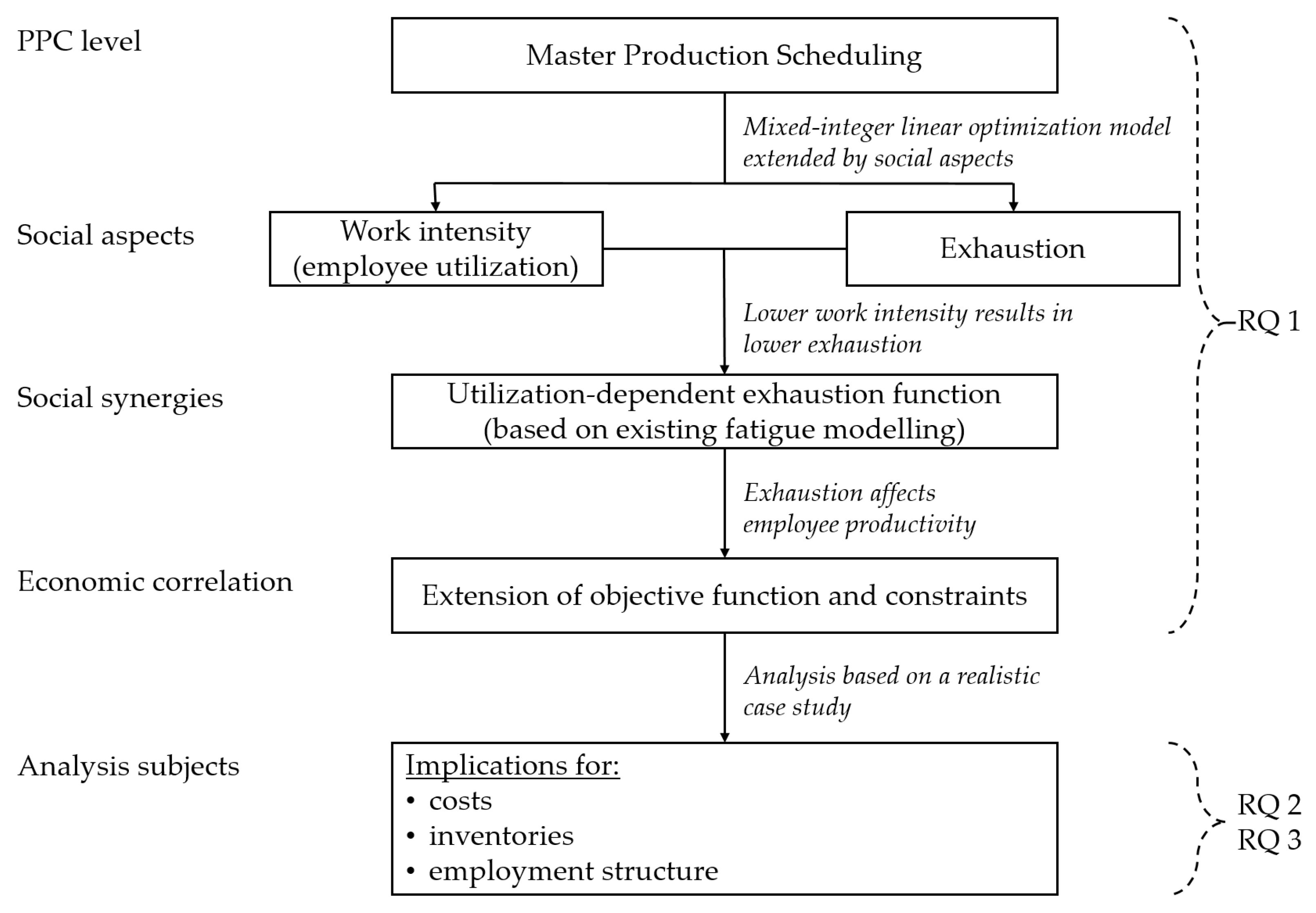
1. Introduction
- RQ 1:
- How can the established description of exhaustion be integrated on an MPS level?
- RQ 2:
- Which cost implications arise due to a reduction in work intensity (employee utilization)?
- RQ 3:
- How will lower exhaustion due to lower work intensity (employee utilization) affect employment structure and pre-production?
2. Literature Review
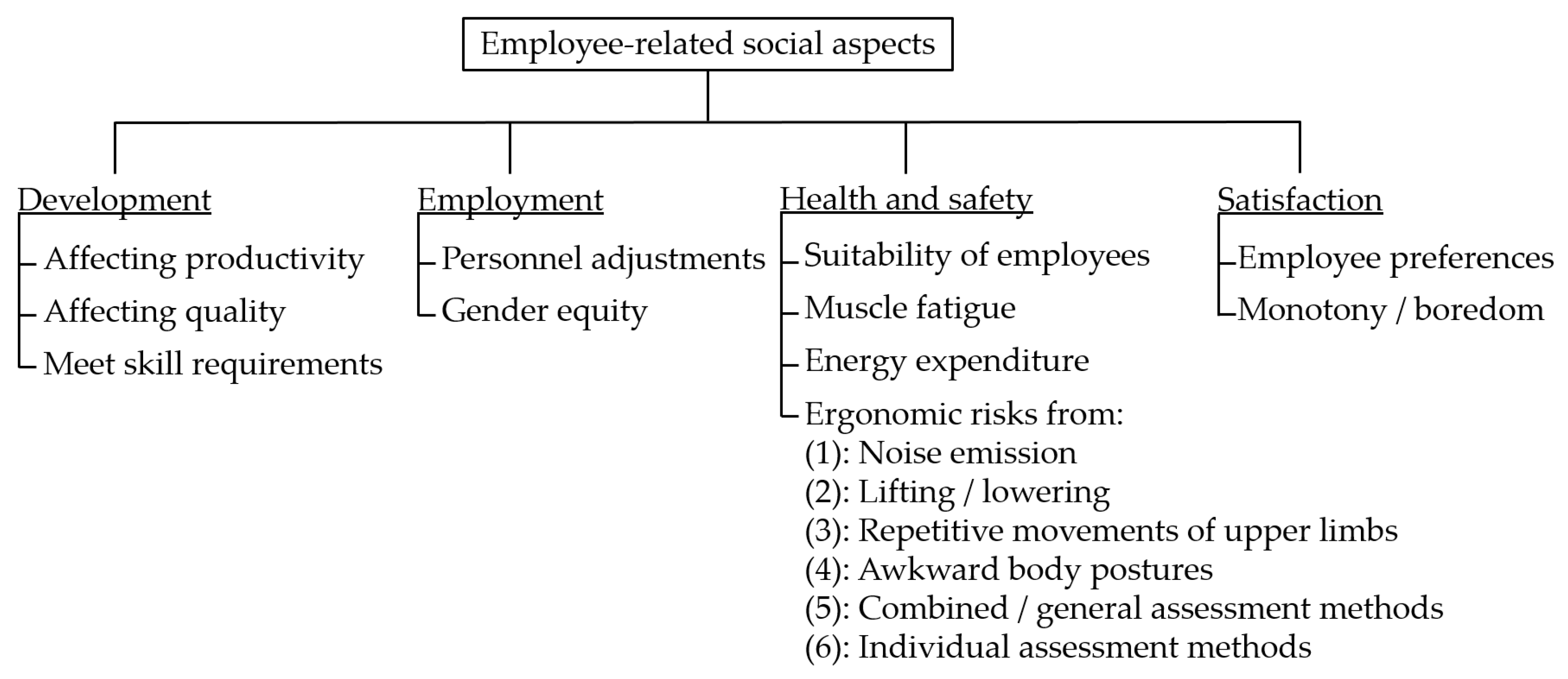
2.1. Employee-Related Social Aspects
2.2. Survey of Existing Approaches
- Employee-related social aspects have rarely been considered at plant level. In this aggregated perspective, longer term planning approaches have not addressed aspects of employee satisfaction and health and safety.
- An analysis of the relationship between social improvements and economic impact is rarely provided. The focus is mainly on the verification of the solution methods applied.
3. MPS with Utilization-Dependant Exhaustion and Subsequent Capacity Requirements
3.1. Optimization Model for MPS Including Employee-Related Social Aspects
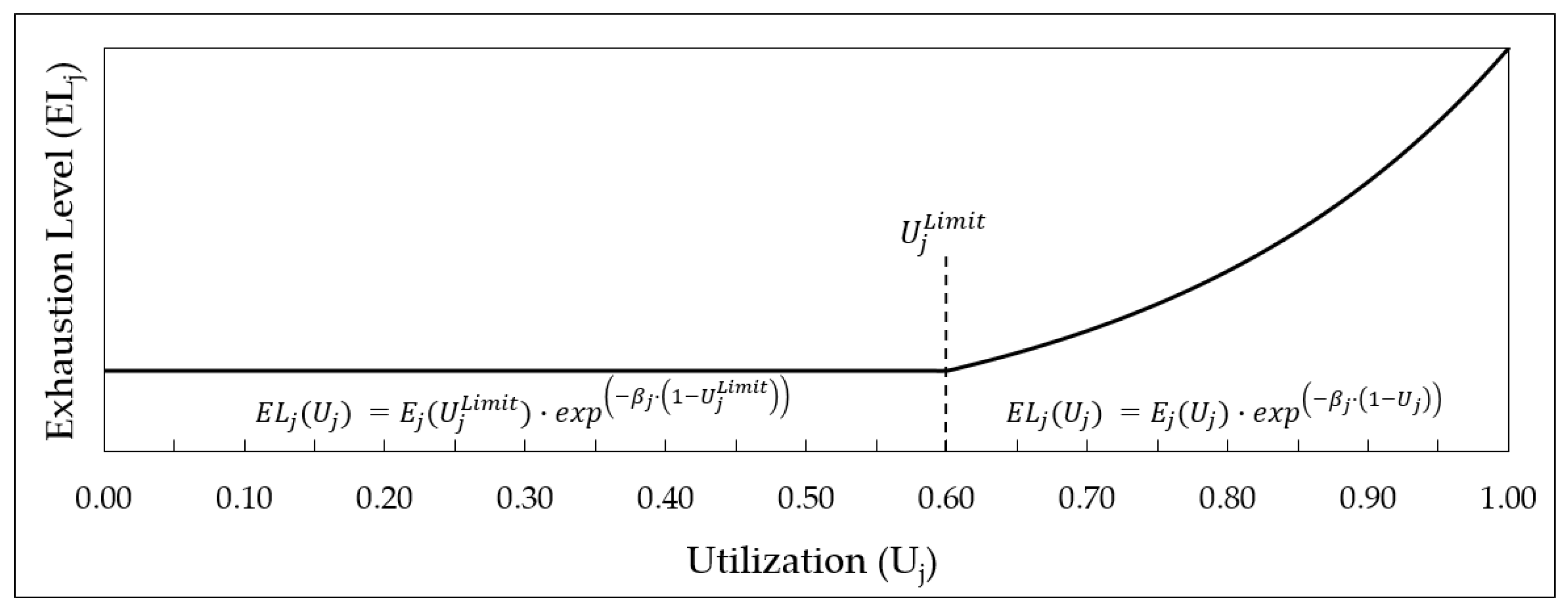
3.2. Exhaustion Modeling
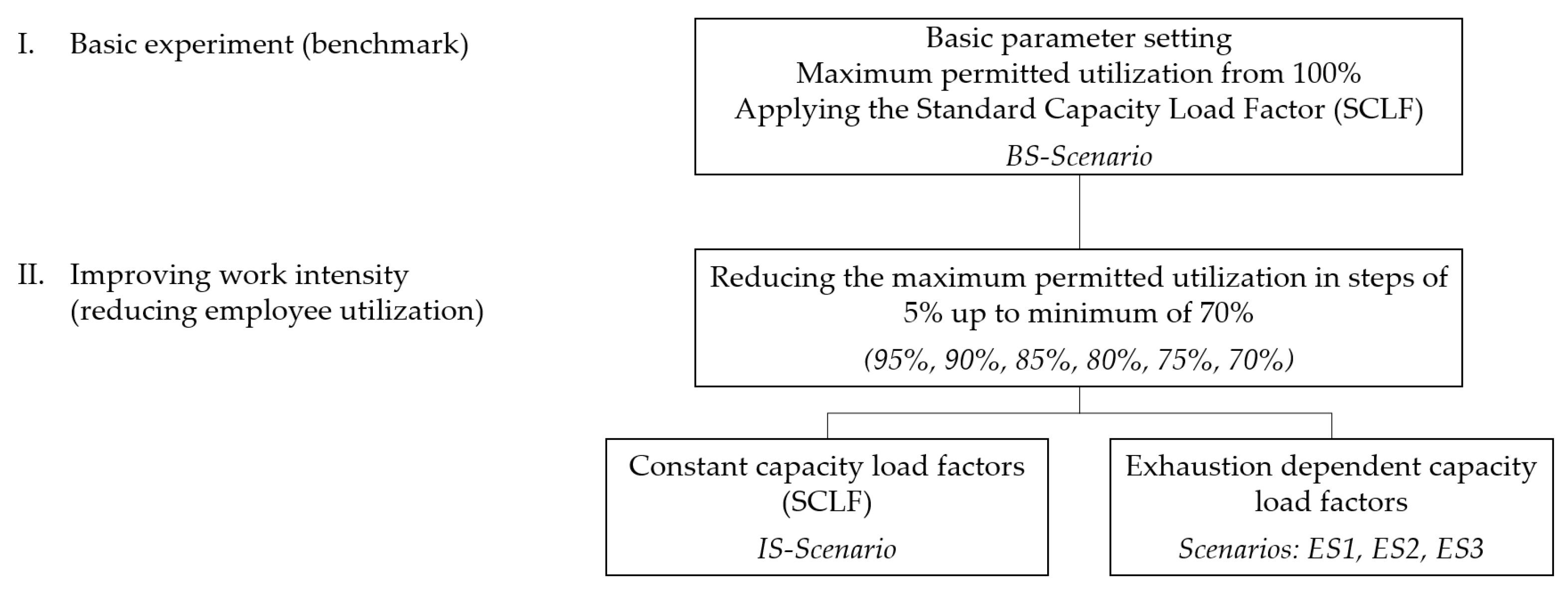
4. Test Problem and Experimental Design
- Constant capacity load factors are applied within the IS scenario. Thereby, for each maximum permitted employee utilization the capacity load factors are equal to the standard-capacity load factors from the BS scenario (). Thus, the benefits of improved work intensity and less exhaustion are not accounted for. With this, we aim to demonstrate the necessity of the more precise (exhaustion-dependent) modelling of employee productivity, like in this approach.
- By applying the exhaustion-dependent capacity load factors, we will account for increasing employee productivity due to reduced exhaustion. For this, in Equation (31), the exhaustion-dependent portion is 75% () which reflects the low level of automation in our case study. Since there are no empirical data for quantifying the exhaustion function so far, we compare three different exhaustion curves (ES1, ES2, ES3). Thereby, we are oriented by the work of ref. [57], who observed a decrease in maximum muscle strength of over 40% in a short-term push test. Due to the low level of automation in our case study, a similar correlation is expected as well. However, we also consider lower correlations. In this respect, we consider the following slow and fast speeds of exhaustion accumulation and exhaustion recovery while the exhaustion level can be reduced up to an employee utilization of 70% ().
- ES1:
- ,
- ES2:
- ,
- ES3:
- ,
For each scenario, the resulting capacity load factors (from Equation (31)) as well as the respective exhaustion factors (from Equation (30)) are given in Table 4. The exhaustion factor reflects the extent to which the exhaustion level is reduced due to the reduced employee utilization. For example, an exhaustion factor of 0.84 means that the exhaustion level is reduced by 16% (compared to the exhaustion level at 100% employee utilization).
5. Results and Discussion
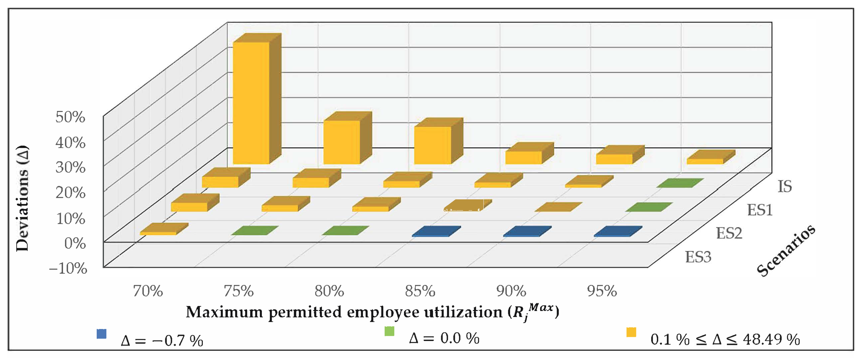
5.1. Cost Implications (RQ2)
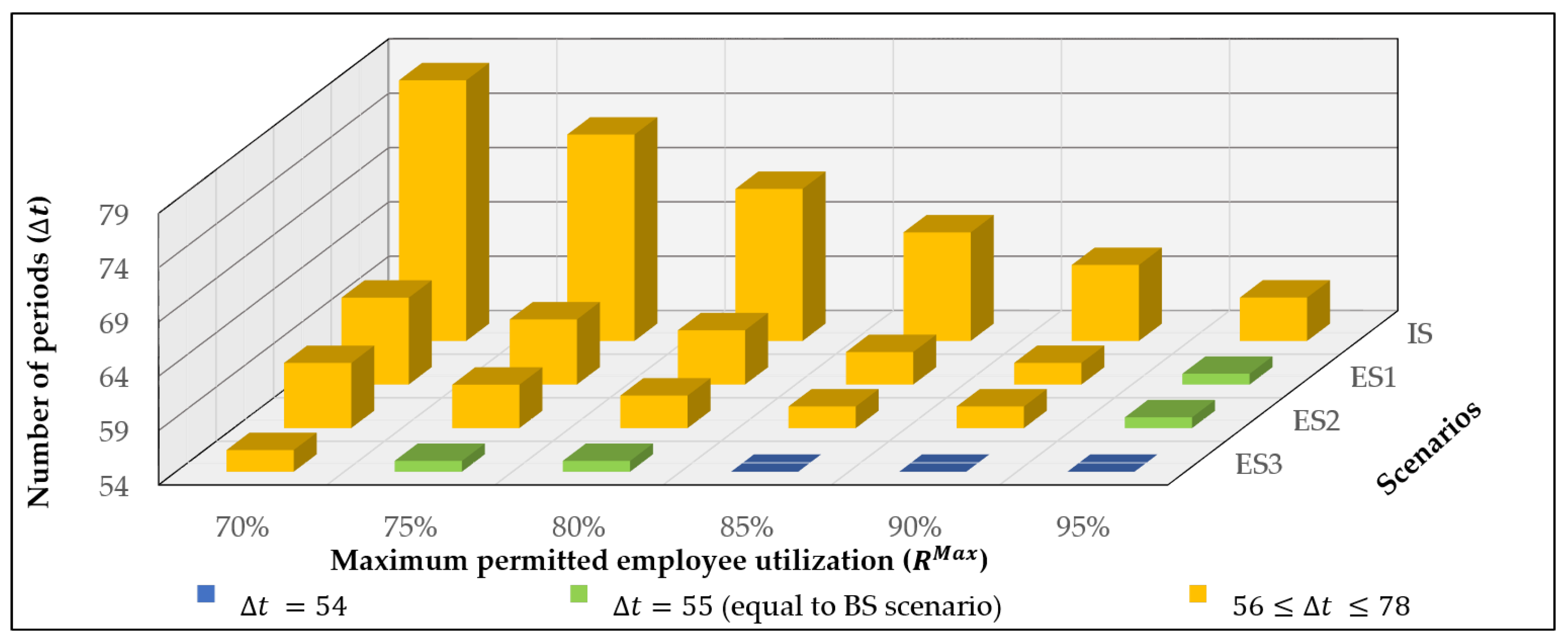
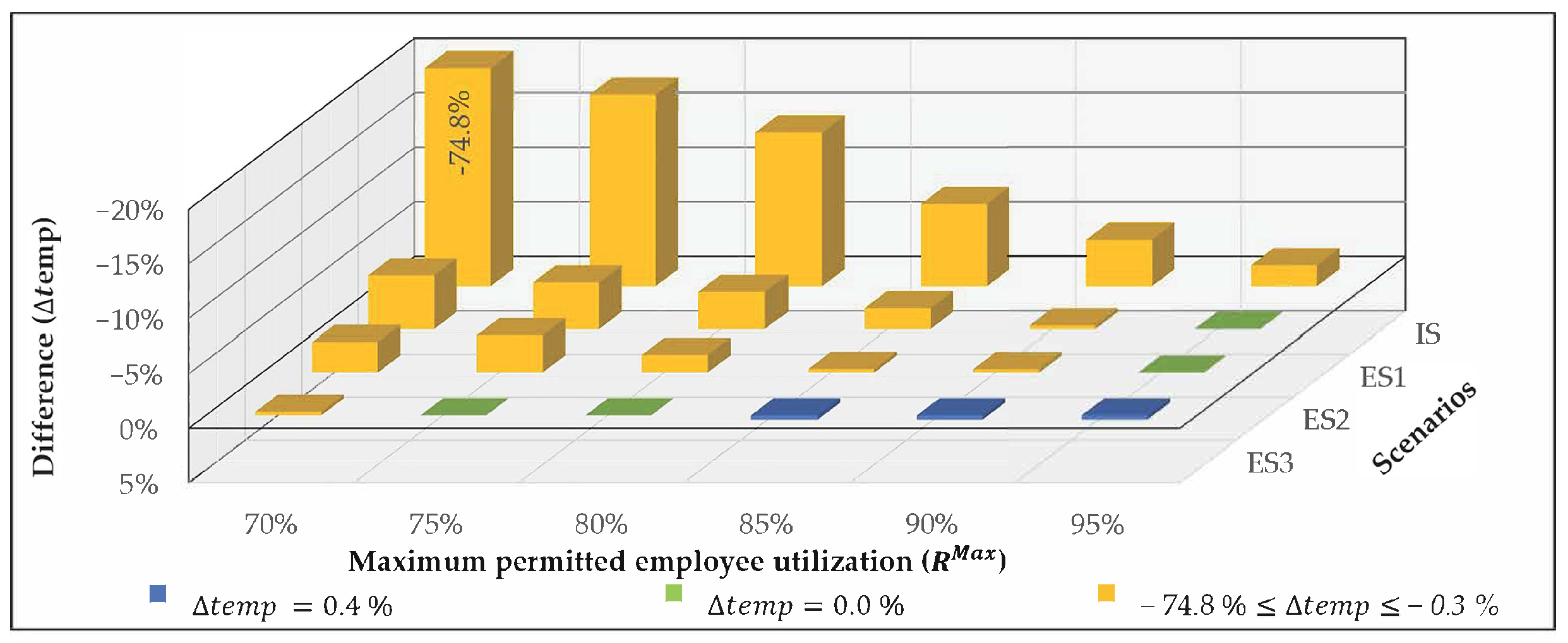
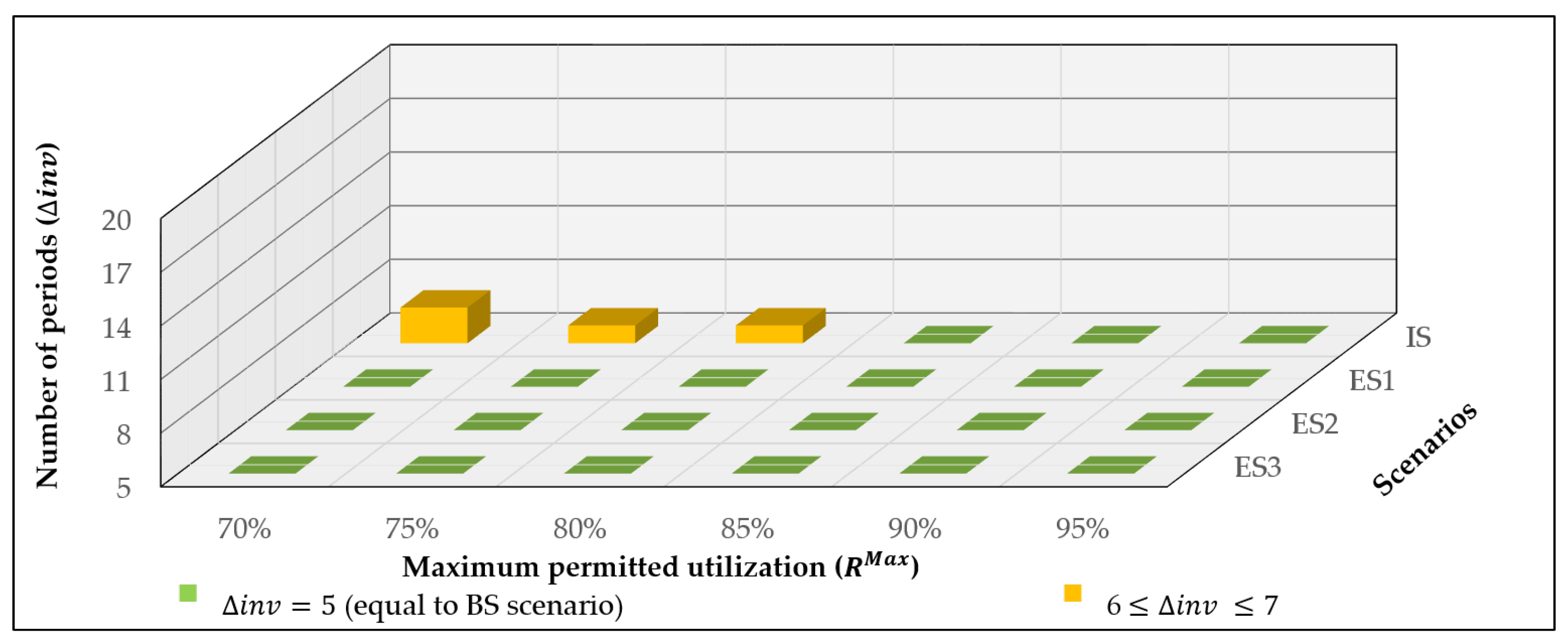
5.2. Implications for Employment Structure and Pre-Production (RQ3)
6. Conclusions
Author Contributions
Funding
Conflicts of Interest
References
- Barker, L.M.; Nussbaum, M.A. Fatigue, performance and the work environment: A survey of registered nurses. J. Adv. Nurs. 2011, 67, 1370–1382. [Google Scholar] [CrossRef] [PubMed]
- Nijp, H.H.; Beckers, D.G.J.; Geurts, S.A.E.; Tucker, P.; Kompier, M.A.J. Systematic review on the association between employee worktime control and work-non-work balance, health and well-being, and job-related outcomes. Scand. J. Work. Environ. Health 2012, 38, 299–313. [Google Scholar] [CrossRef] [PubMed]
- Koziol, L.; Koziol, M. The concept of the trichotomy of motivating factors in the workplace. Cent. Eur. J. Oper. Res. 2020, 28, 707–715. [Google Scholar] [CrossRef]
- International Ergonomics Association. Definition and Domains of Ergonomics. Available online: https://iea.cc/what-is-ergonomics (accessed on 13 December 2022).
- Grosse, E.H.; Calzavara, M.; Glock, C.H.; Sgarbossa, F. Incorporating human factors into decision support models for production and logistics: Current state of research. IFAC-PapersOnLine 2017, 50, 6900–6905. [Google Scholar] [CrossRef]
- Desiderio, E.; García-Herrero, L.; Hall, D.; Segrè, A.; Vittuari, M. Social sustainability tools and indicators for the food supply chain: A systematic literature review. Sustain. Prod. Consum. 2022, 30, 527–540. [Google Scholar] [CrossRef]
- Trost, M.; Claus, T.; Herrmann, F. Social Sustainability in Production Planning: A Systematic Literature Review. Sustainability 2022, 14, 8198. [Google Scholar] [CrossRef]
- Terbrack, H.; Claus, T.; Herrmann, F. Energy-Oriented Production Planning in Industry: A Systematic Literature Review and Classification Scheme. Sustainability 2021, 13, 13317. [Google Scholar] [CrossRef]
- Hax, A.C.; Meal, H.C. Hierarchical integration of production planning and scheduling. In Logistics; Geisler, M.A., Ed.; North-Holland: Amsterdam, The Netherlands, 1975; Volume 1, pp. 53–69. [Google Scholar]
- Drexl, A.; Fleischmann, B.; Günther, H.O.; Stadtler, H.; Tempelmeier, H. Konzeptionelle Grundlagen kapazitätsorientierter PPS-Systeme. Z. Betriebswirtschaftliche Forsch. 1994, 46, 1022–1045. [Google Scholar]
- Herrmann, F.; Manitz, M. Ein hierarchisches Planungskonzept zur operativen Produktionsplanung und -steuerung. In Produktionsplanung und -Steuerung: Forschungsansätze, Methoden und Anwendungen; Claus, T., Herrmann, F., Manitz, M., Eds.; Springer: Berlin, Germany, 2021; pp. 9–25. [Google Scholar] [CrossRef]
- Mateo, M.; Tarral, M.; Rodríguez, P.M.; Galera, A. Ergonomics as basis for a decision support system in the printing industry. Cent. Eur. J. Oper. Res. 2020, 28, 685–706. [Google Scholar] [CrossRef]
- Su, B.; Xie, N. Single workgroup scheduling problem with variable processing personnel. Cent. Eur. J. Oper. Res. 2020, 28, 671–684. [Google Scholar] [CrossRef]
- Choi, G. A goal programming mixed-model line balancing for processing time and physical workload. Comput. Ind. Eng. 2009, 57, 395–400. [Google Scholar] [CrossRef]
- Xu, Z.; Ko, J.; Cochran, D.J.; Jung, M.C. Design of assembly lines with the concurrent consideration of productivity and upper extremity musculoskeletal disorders using linear models. Comput. Ind. Eng. 2012, 62, 431–441. [Google Scholar] [CrossRef]
- Battini, D.; Calzavara, M.; Otto, A.; Sgarbossa, F. The Integrated Assembly Line Balancing and Parts Feeding Problem with Ergonomics Considerations. IFAC-PapersOnLine 2016, 49, 191–196. [Google Scholar] [CrossRef]
- Yoon, S.Y.; Ko, J.; Jung, M.C. A model for developing job rotation schedules that eliminate sequential high workloads and minimize between-worker variability in cumulative daily workloads: Application to automotive assembly lines. Appl. Ergon. 2016, 55, 8–15. [Google Scholar] [CrossRef] [PubMed]
- Akyol, S.D.; Baykasoğlu, A. ErgoALWABP: A multiple-rule based constructive randomized search algorithm for solving assembly line worker assignment and balancing problem under ergonomic risk factors. J. Intell. Manuf. 2019, 30, 291–302. [Google Scholar] [CrossRef]
- Thun, J.H.; Lehr, C.B.; Bierwirth, M. Feel free to feel comfortable—An empirical analysis of ergonomics in the German automotive industry. Int. J. Prod. Econ. 2011, 133, 551–561. [Google Scholar] [CrossRef]
- DGB-Index Gute Arbeit. Der Report 2013. Wie Die Beschäftigten Die Arbeitsbedingungen in Deutschland Beurteilen: Mit dem Themenschwerpunkt: Unbezahlte Arbeit; Institut DGB-Index Gute Arbeit: Berlin, Germany, 2014. [Google Scholar]
- Ahlers, E. Work and Health in German Companies. Findings from the WSI Works Councils Survey 2015; Report No. 33e; WSI Institute of Economic and Social Research: Düsseldorf, Germany, 2017. [Google Scholar]
- World Commission on Environment Development. Our Common Future (the Brundtland Report); Oxford University Press: New Delhi, India, 1987. [Google Scholar]
- Neri, A.; Cagno, E.; Lepri, M.; Trianni, A. A triple bottom line balanced set of key performance indicators to measure the sustainability performance of industrial supply chains. Sustain. Prod. Consum. 2021, 26, 648–691. [Google Scholar] [CrossRef]
- Joung, C.B.; Carrell, J.; Sarkar, P.; Feng, S.C. Categorization of indicators for sustainable manufacturing. Ecol. Indic. 2013, 24, 148–157. [Google Scholar] [CrossRef]
- GRI. Global Reporting Initiative; GRI: Boston, MA, USA, 2022. [Google Scholar]
- Boenzi, F.; Mossa, G.; Mummolo, G.; Romano, V.A. Workforce Aging in Production Systems: Modeling and Performance Evaluation. Procedia Eng. 2015, 100, 1108–1115. [Google Scholar] [CrossRef]
- Nerdinger, F.W.; Blickle, G.; Schaper, N. Arbeits- und Organisationspsychologie, 4th ed.; Springer: Berlin/Heidelberg, Germany, 2019. [Google Scholar] [CrossRef]
- Jaber, M.Y.; Givi, Z.S.; Neumann, W.P. Incorporating human fatigue and recovery into the learning–forgetting process. Appl. Math. Model. 2013, 37, 7287–7299. [Google Scholar] [CrossRef]
- Neumann, W.P.; Dul, J. Human factors: Spanning the gap between OM and HRM. Int. J. Oper. Prod. Manag. 2010, 30, 923–950. [Google Scholar] [CrossRef]
- Yeow, J.A.; Ng, P.K.; Tan, K.S.; Chin, T.S.; Lim, W.Y. Effects of Stress, Repetition, Fatigue and Work Environment on Human Error in Manufacturing Industries. J. Appl. Sci. 2014, 14, 3464–3471. [Google Scholar] [CrossRef]
- Hasselhorn, H.M. Arbeit, Stress und Krankheit. In Psychosoziale Gesundheit im Beruf; Weber, A., Hörmann, G., Ferreira, Y., Eds.; Gentner: Stuttgart, Germany, 2007; pp. 47–73. [Google Scholar]
- Battini, D.; Delorme, X.; Dolgui, A.; Persona, A.; Sgarbossa, F. Ergonomics in assembly line balancing based on energy expenditure: A multi-objective model. Int. J. Prod. Res. 2016, 54, 824–845. [Google Scholar] [CrossRef]
- Bautista, J.; Batalla-García, C.; Alfaro-Pozo, R. Models for assembly line balancing by temporal, spatial and ergonomic risk attributes. Eur. J. Oper. Res. 2016, 251, 814–829. [Google Scholar] [CrossRef]
- Kara, Y.; Atasagun, Y.; Gökçen, H.; Hezer, S.; Demirel, N. An integrated model to incorporate ergonomics and resource restrictions into assembly line balancing. Int. J. Comput. Integr. Manuf. 2014, 27, 997–1007. [Google Scholar] [CrossRef]
- Baykasoğlu, A.; Tasan, S.O.; Tasan, A.S.; Akyol, S.D. Modeling and solving assembly line design problems by considering human factors with a real-life application. Hum. Factors Ergon. Manuf. Serv. Ind. 2017, 27, 96–115. [Google Scholar] [CrossRef]
- Mossa, G.; Boenzi, F.; Digiesi, S.; Mummolo, G.; Romano, V.A. Productivity and ergonomic risk in human based production systems: A job-rotation scheduling model. Int. J. Prod. Econ. 2016, 171, 471–477. [Google Scholar] [CrossRef]
- Song, J.B.; Lee, C.; Lee, W.J.; Bahn, S.; Jung, C.J.; Yun, M.H. Development of a job rotation scheduling algorithm for minimizing accumulated work load per body parts. Work (Read. Mass.) 2016, 53, 511–521. [Google Scholar] [CrossRef]
- Nanthavanij, S.; Yaoyuenyong, S.; Jeenanunta, C. Heuristic approach to workforce scheduling with combined safety and productivity objective. Int. J. Ind. Eng. Theory Appl. Pract. 2010, 17, 319–333. [Google Scholar] [CrossRef]
- Battini, D.; Glock, C.H.; Grosse, E.H.; Persona, A.; Sgarbossa, F. Ergo-lot-sizing: An approach to integrate ergonomic and economic objectives in manual materials handling. Int. J. Prod. Econ. 2017, 185, 230–239. [Google Scholar] [CrossRef]
- Zadjafar, M.A.; Gholamian, M.R. A sustainable inventory model by considering environmental ergonomics and environmental pollution, case study: Pulp and paper mills. J. Clean. Prod. 2018, 199, 444–458. [Google Scholar] [CrossRef]
- Cai, M.; Shen, Q.W.; Luo, X.G.; Huang, G. Improving sustainability in combined manual material handling through enhanced lot-sizing models. Int. J. Ind. Ergon. 2020, 80, 103008. [Google Scholar] [CrossRef]
- Otto, A.; Battaïa, O. Reducing physical ergonomic risks at assembly lines by line balancing and job rotation: A survey. Comput. Ind. Eng. 2017, 111, 467–480. [Google Scholar] [CrossRef]
- Mirzapour Al-E-Hashem, S.M.J.; Malekly, H.; Aryanezhad, M.B. A multi-objective robust optimization model for multi-product multi-site aggregate production planning in a supply chain under uncertainty. Int. J. Prod. Econ. 2011, 134, 28–42. [Google Scholar] [CrossRef]
- Khalili-Damghani, K.; Shahrokh, A. Solving a new multi-period multi-objective multi-product aggregate production planning problem using fuzzy goal programming. Ind. Eng. Manag. Syst. 2014, 13, 369–382. [Google Scholar] [CrossRef]
- Gholamian, N.; Mahdavi, I.; Tavakkoli-Moghaddam, R. Multi-objective multi-product multi-site aggregate production planning in a supply chain under uncertainty: Fuzzy multi-objective optimisation. Int. J. Comput. Integr. Manuf. 2016, 19, 1–17. [Google Scholar] [CrossRef]
- Aziz, R.A.; Paul, H.K.; Karim, T.M.; Ahmed, I.; Azeem, A. Modeling and optimization of multilayer aggregate production planning. J. Oper. Supply Chain. Manag. 2018, 11, 1–15. [Google Scholar] [CrossRef]
- Madadi, N.; Wong, K.Y. A Multiobjective Fuzzy Aggregate Production Planning Model Considering Real Capacity and Quality of Products. Math. Probl. Eng. 2014, 2014, 313829. [Google Scholar] [CrossRef]
- Günther, H.O.; Tempelmeier, H. Produktion und Logistik: Supply Chain und Operations Management, 12th ed.; BoD-Books on Demand: Norderstedt, Germany, 2016. [Google Scholar]
- El ahrache, K.; Imbeau, D.; Farbos, B. Percentile values for determining maximum endurance times for static muscular work. Int. J. Ind. Ergon. 2006, 36, 99–108. [Google Scholar] [CrossRef]
- Jamalnia, A.; Soukhakian, M.A. A hybrid fuzzy goal programming approach with different goal priorities to aggregate production planning. Comput. Ind. Eng. 2009, 56, 1474–1486. [Google Scholar] [CrossRef]
- Mazzola, J.B.; Neebe, A.W.; Rump, C.M. Multiproduct production planning in the presence of work-force learning. Eur. J. Oper. Res. 1998, 106, 336–356. [Google Scholar] [CrossRef]
- Trost, M.; Teich, E.; Claus, T.; Herrmann, F. Ein lineares Optimierungsmodell zur Hauptproduktionsprogrammplanung mit Berücksichtigung sozialer Größen. uwf UmweltWirtschaftsForum 2017, 25, 71–80. [Google Scholar] [CrossRef]
- Trost, M. Master Production Scheduling With Integrated Aspects of Personnel Planning and Consideration of Employee Utilization Specific Processing Times. In Proceedings of the 32nd International ECMS Conference on Modelling and Simulation, ECMS 2018, Wilhelmshaven, Germany, 22–26 May 2018; pp. 329–335. [Google Scholar] [CrossRef]
- Trost, M.; Claus, T.; Herrmann, F. Adapted Master Production Scheduling: Potential For Improving Human Working Conditions. In Proceedings of the 33rd International ECMS Conference on Modelling and Simulation, ECMS 2019, Caserta, Italy, 11–14 June 2019; pp. 310–316. [Google Scholar] [CrossRef]
- IG Metall. ERA-Monatsentgelte ab April 2018; IG Metall: Stuttgart, Germany, 2019. [Google Scholar]
- IG Metall. Zuschläge für Mehr-, Schicht-, Nacht-, Sonn- und Feiertagsarbeit; IG Metall: Stuttgart, Germany, 2019. [Google Scholar]
- Zhang, Z.; Li, K.W.; Zhang, W.; Ma, L.; Chen, Z. Muscular fatigue and maximum endurance time assessment for male and female industrial workers. Int. J. Ind. Ergon. 2014, 44, 292–297. [Google Scholar] [CrossRef]


| Sets | |
| Set of employee groups () | |
| J | Set of production segments () |
| K | Set of products () |
| S | Set of shift models () |
| T | Set of time periods () |
| Z | Set of lead-time periods for capacity load () |
| Parameters | |
| Parameter that controls the speed of exhaustion accumulation in production segment j | |
| Parameter that controls the speed of exhaustion recovery in production segment j | |
| Available capacity per period and employee of an employee group | |
| Demand per product k and period t | |
| , | Capacity load factor for lead-time period z, production segment j and product k |
| Inventory holding costs per unit and period of product k | |
| Initial inventory level per product k | |
| Maximum inventory level per product k | |
| Cost rate for hiring an employee from employee group | |
| Exhaustion-dependent portion of capacity load factors in production segment j | |
| Cost rate for employee turnover per employee from employee group | |
| Maximum permitted employee utilization in production segment j | |
| Factor for calculating shift surcharges for using shift model s | |
| Maximum number of employees per production segment j in shift model s | |
| Minimum number of employees per production segment j in shift model s | |
| Cost rate per employee from employee group in production segment j | |
| Initial number of employees from employee group in production segment j and shift model s | |
| Maximum number of employees from employee group in production segment j | |
| Minimum number of employees from employee group in production segment j | |
| Maximum number of employees in production segment j | |
| Minimum number of employees in production segment j | |
| Minimum employee utilization in production segment j below which exhaustion not decrease | |
| Lead-time periods for hiring employees from employee group | |
| Lead-time periods for employee turnover from employee group | |
| Decision variables | |
| Available capacity per production segment j in period t | |
| Capacity requirement per production segment j in period t | |
| Accumulated exhaustion at employee utilization in production segment j | |
| Exhaustion factor (normalized exhaustion level) in production segment j | |
| Exhaustion level after exhaustion accumulation and exhaustion recovery in production segment j | |
| Exhaustion-dependent capacity load factor for lead-time period z, production segment j and product k | |
| Inventory level per product k in period t | |
| Number of hired employees from employee group in production segment j and period t | |
| Amount of employee turnover from employee group in production segment j and period t | |
| Boolean variable for selection of the used shift model per production segment j, shift model s and period t | |
| Number of employees from employee group in production segment j, shift model s and period t | |
| Employee utilization (work intensity) in production segment j | |
| Production quantity per product k in period t | |
| Employee Group () | [in seconds] | [in ] | [in ] | [in ] |
|---|---|---|---|---|
| 405,000 | 3671 | 15,000 | 40,000 | |
| 300,000 | 5692 | 1500 | 100 |
| Shift Model (S) | |||
|---|---|---|---|
| 0 | 2000 | 0.00% | |
| 2001 | 4000 | 0.00% | |
| 4001 | 6000 | 8.33% |
| Utilization () | Product (K) | [in seconds] | [in seconds] | [in seconds] | |||
|---|---|---|---|---|---|---|---|
| 95% | 0.95 | 0.94 | 0.93 | 13,479 | 13,403 | 13,233 | |
| 10,591 | 10,531 | 10,397 | |||||
| 90% | 0.90 | 0.89 | 0.86 | 12,981 | 12,827 | 12,519 | |
| 10,200 | 10,078 | 9836 | |||||
| 85% | 0.86 | 0.84 | 0.80 | 12,505 | 12,268 | 11,854 | |
| 9825 | 9639 | 9314 | |||||
| 80% | 0.81 | 0.78 | 0.74 | 12,047 | 11,726 | 11,234 | |
| 9466 | 9214 | 8827 | |||||
| 75% | 0.77 | 0.73 | 0.68 | 11,607 | 11,199 | 10,654 | |
| 9120 | 8799 | 8371 | |||||
| 70% | 0.73 | 0.68 | 0.63 | 11,181 | 10,684 | 10,111 | |
| 8785 | 8394 | 7944 |
| Variable | Scenario | Maximum Permitted Employee Utilization () | ||||||
|---|---|---|---|---|---|---|---|---|
| 100% | 95% | 90% | 85% | 80% | 75% | 70% | ||
| Average employee utilization | BS | 99.33% | ||||||
| IS | 94.38% | 89.42% | 84.46% | 79.52% | 74.56% | 69.56% | ||
| ES1 | 94.36% | 89.41% | 84.45% | 79.48% | 74.52% | 69.56% | ||
| ES2 | 94.36% | 89.40% | 84.44% | 79.48% | 74.51% | 69.55% | ||
| ES3 | 94.36% | 89.39% | 84.42% | 79.46% | 74.50% | 69.54% | ||
| Total costs | BS | 616,564,291 | ||||||
| IS | +5.22% | +11.01% | +17.49% | + 24.78% | +33.03% | +42.57% | ||
| ES1 | +1.34% | +3.00% | +5.04% | +7.50% | +10.45% | +13.97% | ||
| ES2 | +0.77% | +1.78% | +3.07% | +4.66% | +6.60% | +8.94% | ||
| ES3 | −0.50% | −0.64% | −0.39% | +0.30% | +1.46% | +3.15% | ||
| Variable | Scenario | Maximum Permitted Utilization () | ||||||
|---|---|---|---|---|---|---|---|---|
| 100% | 95% | 90% | 85% | 80% | 75% | 70% | ||
| Average number of core employees | BS | 2748 | ||||||
| IS | +5.25% | +11.09% | +17.63% | +24.96% | +33.28% | +43.07% | ||
| ES1 | +1.35% | +3.01% | +5.07% | +7.55% | +10.52% | +14.06% | ||
| ES2 | +0.78% | +1.80% | +3.08% | +4.68% | +6.64% | +8.99% | ||
| ES3 | −0.50% | −0.64% | −0.38% | +0.30% | +1.47% | +3.16% | ||
| Expected change | IS | +5.26% | +11.11% | +17.65% | +25.00% | +33.33% | +42.86% | |
| ES1 | +1.35% | +3.03% | +5.08% | +7.56% | +10.54% | +14.09% | ||
| ES2 | +0.78% | +1.80% | +3.10% | +4.70% | +6.66% | +9.02% | ||
| ES3 | − 0.50% | −0.64% | −0.39% | +0.30% | +1.47% | +3.17% | ||
Disclaimer/Publisher’s Note: The statements, opinions and data contained in all publications are solely those of the individual author(s) and contributor(s) and not of MDPI and/or the editor(s). MDPI and/or the editor(s) disclaim responsibility for any injury to people or property resulting from any ideas, methods, instructions or products referred to in the content. |
© 2023 by the authors. Licensee MDPI, Basel, Switzerland. This article is an open access article distributed under the terms and conditions of the Creative Commons Attribution (CC BY) license (https://creativecommons.org/licenses/by/4.0/).
Share and Cite
Trost, M.; Claus, T.; Herrmann, F. Master Production Scheduling with Consideration of Utilization-Dependent Exhaustion and Capacity Load. Sustainability 2023, 15, 6816. https://doi.org/10.3390/su15086816
Trost M, Claus T, Herrmann F. Master Production Scheduling with Consideration of Utilization-Dependent Exhaustion and Capacity Load. Sustainability. 2023; 15(8):6816. https://doi.org/10.3390/su15086816
Chicago/Turabian StyleTrost, Marco, Thorsten Claus, and Frank Herrmann. 2023. "Master Production Scheduling with Consideration of Utilization-Dependent Exhaustion and Capacity Load" Sustainability 15, no. 8: 6816. https://doi.org/10.3390/su15086816
APA StyleTrost, M., Claus, T., & Herrmann, F. (2023). Master Production Scheduling with Consideration of Utilization-Dependent Exhaustion and Capacity Load. Sustainability, 15(8), 6816. https://doi.org/10.3390/su15086816