Article

Optimizing Extreme Learning Machine for Drought Forecasting: Water Cycle vs. Bacterial Foraging

1
Department of Civil Engineering, Antalya Bilim University, Antalya 07190, Turkey
2
Centre of Excellence in Hydroinformatics, Faculty of Civil Engineering, University of Tabriz, Tabriz 51666, Iran
3
Department of Civil Engineering, Akdeniz University, Antalya 07070, Turkey
4
Department of Information Technology, Choman Technical Institute, Erbil Polytechnic University, Erbil 44001, Iraq
5
Department of Civil Engineering, Inonu University, Inonu 44280, Turkey
6
Faculty of Civil and Environmental Engineering, Near East University, Lefkoşa 99138, Turkey
7
Department of Civil Engineering, Payame Noor University, Tabriz Branch, Tabriz 51748, Iran
8
Department of Physical Geography and Ecosystem Science, Lund University, Sölvegatan 12, SE-223 62 Lund, Sweden
*
Author to whom correspondence should be addressed.
Sustainability 2023, 15(5), 3923; https://doi.org/10.3390/su15053923
Submission received: 5 October 2022 / Revised: 8 January 2023 / Accepted: 16 January 2023 / Published: 21 February 2023
(This article belongs to the Special Issue Drought and Sustainable Water Management)

Abstract

:
Machine learning (ML) methods have shown noteworthy skill in recognizing environmental patterns. However, presence of weather noise associated with the chaotic characteristics of water cycle components restricts the capability of standalone ML models in the modeling of extreme climate events such as droughts. To tackle the problem, this article suggests two novel hybrid ML models based on combination of extreme learning machine (ELM) with water cycle algorithm (WCA) and bacterial foraging optimization (BFO). The new models, respectively called ELM-WCA and ELM-BFO, were applied to forecast standardized precipitation evapotranspiration index (SPEI) at Beypazari and Nallihan meteorological stations in Ankara province (Turkey). The performance of the proposed models was compared with those the standalone ELM considering root mean square error (RMSE), Nash-Sutcliffe efficiency (NSE), and graphical plots. The forecasting results for three- and six-month accumulation periods showed that the ELM-WCA is superior to its counterparts. The NSE results of the SPEI-3 forecasting in the testing period proved that the ELM-WCA improved drought modeling accuracy of the standalone ELM up to 72% and 85% at Beypazari and Nallihan stations, respectively. Regarding the SPEI-6 forecasting results, the ELM-WCA achieved the highest RMSE reduction percentage about 63% and 56% at Beypazari and Nallihan stations, respectively.

1. Introduction

Attributable to climate change, the extent and frequency of extreme weather events are changing at both local and global scales so that an increase in the severity and intensity of drought in arid and semi-arid regions has been projected [1]. Considering the duration of rainfall deficit, drought is often categorized into four classes: meteorological, agricultural, hydrologic, and socioeconomic [2]. When a natural ecosystem is injured by water deficit, this extreme condition is called ecological drought [3]. Each class has own detecting variables such as precipitation and temperature for meteorological drought [4], evaporation stress and soil moisture for agricultural drought [5], surface and subsurface water shortage for hydrological one [6], resilience of inflow-demand and water storage for socioeconomic drought [7], and difference between ecological water requirement and consumption for ecological drought [8]. As these parameters, particularly water cycle components, are highly nonlinear and non-stationary in nature, the associated drought indices have chaotic characteristics, and hence are challenging to model and forecast [9,10].
One of the most frequently asked questions in sustainable water resources management and operation is: “How often does a drought occur?” The answer to these questions is important since it determines the amount of time that we need to bridge with current water resources. Surprisingly, several approaches exist to model and predict a drought occurrence. The relevant literature shows that drought prediction models are broadly categorized into three groups: (a) physically-based (dynamical) models [11,12]; (b) statistical models including data-driven and machine learning (ML) models [13,14,15,16]; and (c) hybrid statistical–dynamical techniques [17]. Status and prospects of each type were elaborately discussed in [18] highlighting a growing tendency to use multiple models and combine their forecasts.
Fundamentals of several ML methods and their potential applications in drought forecasting have been reviewed in a recent study [10] demonstrating that an efficient drought mitigation plan and adaptation strategy needs an efficient drought forecasting model. Among stochastic, probabilistic, and ML approaches, the study has concluded that the ML approaches provide more accurate and efficient models. Given that ML methods are, by definition, data-driven, they simply capture short-term evolution of the underlying manifold. Such models, however, do not capture and explain extreme phenomena including both wet and dry extremes [19]. Regarding meteorological drought prediction in Iran, a study showed that artificial neural networks (ANNs) could be used for Standardized Precipitation Index (SPI) and Effective Drought Index prediction in Iran [20]. Satisfactory implementation of the group method of data handling, adaptive neuro-fuzzy inference system (ANFIS), generalized regression neural network, least square-support vector machine models, and ANFIS coupled with three nature-inspired optimization algorithm models for multivariate standardized precipitation index prediction in Iran were also reported by [13]. Another article demonstrated that extreme learning machine (ELM) can be used for Standardized Precipitation Evapotranspiration Index (SPEI) prediction in eastern Australia [16]. The study revealed that ELM outperforms ANN in their study area. The ANN and XGBoost methods were used for SPEI prediction using hydroclimatological predictors and showed that XGBoost outperforms ANN [21]. More recently, [22] compared the efficiency of ELM, random forest, and support vector machine models for SPEI prediction in different basins and showed that a precise forecasting model can be developed via the use of sea surface temperature as an SPEI predictor.
The purpose of any supervised ML algorithm is to get low bias and low variance. Linear ML algorithms, which assume a linear relationship between the inputs and the output variable, generally have a high bias but a low variance. In contrast, nonlinear ML algorithms, such as ANNSs and ELMs, usually have a low bias but a high variance. Thus, the parameterization of nonlinear ML algorithms often needs a trade-off to balance out bias and variance. Recent studies have indicated that different factors such as bias-variance tradeoff and number of training data may alter the performance of nonlinear supervised ML methods [10]. In addition, they might get trapped in local optimum when classic gradient-based algorithms are used to train them [23,24]. To cope with these problems, recent studies have attempted to develop hybrid ML models in which either an optimization algorithm is utilized for structural improvement of the desired model [25,26] or an effective data pre-processing approach is used to denoise or transform raw predictor variables (inputs) to more effective ones [27,28]. In the present study, the former approach is taken to develop two novel hybrid ML models based on a combination of ELM with two emerging optimization algorithms, namely bacterial foraging optimization (BFO [29]) and water cycle algorithm (WCA [30]) to investigate how much these bio-inspired techniques can improve the forecasting accuracy of ELM-based SPEI prediction model. To this end, we used 46 years (1971–2016) near surface air temperature and precipitation datasets from two synoptic stations in Ankara province, Turkey. Then, the SPEI time series in two accumulation times (3-month and 6-month) were calculated and modeled using the attained SPEI time series. Finally, a comparative analysis among these hybrid models (i.e., ELM-BFO and ELM-WCA) and the standalone ELM was performed. It is worth mentioning that the evolved hybrid algorithms are, in fact, nonlinear approximations of the short-term evolution of the system; however, we call them models throughout this study.
Although WCA and BFO algorithms have been effectively used to optimize a variety of ML models in different problems [31,32,33], current literature has indicated that SPEI forecasting using hybrid ELM-BFO and ELM-WCA models have not been explored yet. Therefore, the main contributions of this study are twofold. First, for the first time, the study demonstrates predictive capabilities of these hybrid models for SPEI forecasting in two accumulation times. Second, a comprehensive comparison among these hybrid models and the standalone ELM is presented for the case study area. The rest of this paper is organized as below: Section 2 provides the information required for SPEI calculation at each region. Section 3 the details of the proposed hybrid methods. In Section 4 and Section 5, the forecasting results/comparisons and the conclusions are presented, respectively.

2. Materials and Methods

2.1. SPEI Calculation Using the Ground Truth Data

The SPEI is a meteorological drought indicator that takes both precipitation and temperature data into account to characterize spatial and temporal drought condition [34]. The index is suitable for monitoring and predicting drought under different type of climates [35]. To calculate SPEI, climatic water balance, also known as deficit, is first calculated via subtracting potential evapotranspiration from precipitation at each month and then, a desired distribution model is fitted to monthly moisture deficit. The months with negative SPEI values are considered as dry months. When log-logistic function is selected as the desired distribution model, SPEI values in the range [−1.1 to −1.42], [−1.43 to −1.23], and less than −1.83 respectively represent the moderate, severe, and extreme drought events [36].
To attain SPEI series, long-term precipitation, and temperature data (from 1971 to 2016) at Beypazari and Nallihan synoptic stations (Figure 1) were used. As shown in Figure 2, we considered three- and six-months accumulation periods so that all the training and verification tasks will be done for SPEI-3 and SPEI-6, separately.

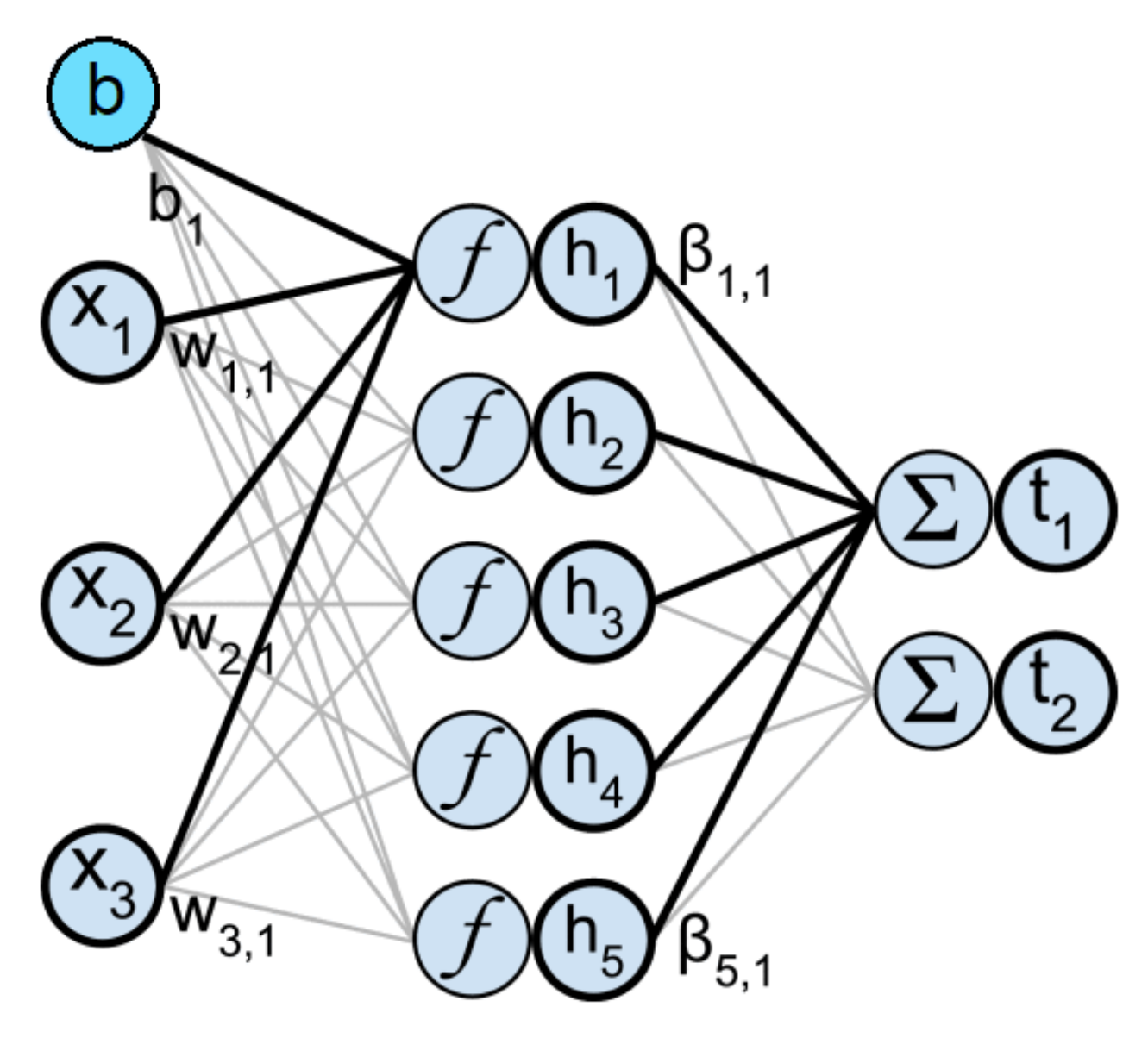
2.2. The Benchmark ELM Model

Despite various effective implementations of regular neural networks [37] such as feedforwards, they are criticized because parameter adjustment requires so much time [38]. In case of complicated systems, use of parameter optimization and data pre-processing techniques to obtain the best ANN structure/inputs could be necessary. Huang et al. [38] recommended a novel neural training method, called ELM, to solve such drawbacks. It applies an innovative feed-forward ANN algorithm having greater generalization capabilities and more speed than ordinary feed-forward neural networks. In fact, ELM has a single hidden layer in which the weights W and bias b of its input layer (see Figure 3) are set randomly and remain unchanged during its training process. As the input weights remain constant, the output weights (denoted by β in the figure) are independent of them and are directly determined without iteration. This is the reason responsible for ELM’s accelerated learning process [39]. As illustrated in Figure 3, the relation between the inputs ( X i i ) and outputs ( t i ) is expressed by Equation (1) in which f is the activation function (sigmoid function in the present study).
t i + ε i = j = 1 L β j f W j X i + b j
where f is a user-defined activation function (the sigmoid function was used in the present study), L is the number of hidden neurons and i indicates an individual input in the training set.
In this study, ELM was simply coded in MATLB and was trained using the training data set of each meteorology station. As the SPEI signals vary in the limited range [–3, 3], the hidden weights and bias were selected using the empirical randomization function in the range [−1, 1], and the number of hidden neurons was determined via a trial-error procedure. Such ELMs are sub-optimal and might produce a high variance error as we previously mentioned. Thus, optimizing the matrix of weights and biases of the ELM trough WCA and BFO algorithms was investigated in this study.

2.3. Water Cycle Algorithm

The WCA is a relatively new algorithm that uses the conceptual formulation of the hydrological water cycle to determine the optimal solution for parameter optimization problems [30]. The algorithm is based on the interconnectedness of streams, rivers, and a sea [40,41]. The initial assumption is that a population of raindrops is generated at random by a rainfall process, and the best raindrop is the one that produces the best fitness (i.e., minimum cost function) [41,42]. Streams, rivers, and the sea are labeled as “good or the best raindrops” based on their performance compared to the other raindrops. The best raindrop is selected as a sea and a river is considered as a good raindrop, and the rest of drops are called streams [41]. Like nature, streams flow towards the river and rivers flow to the sea. The algorithm can be used to solve any Nvar-dimensional optimization problem [30].
To begin the optimization, the initial population of randomly distributed raindrops (i.e., candidate solution matrix X) is made with the dimensions Npop × Nvar.
Population   of   Raindrops = Raindrop 1 Raindrop 2 Raindrop 3 Raindrop N pop = x 1 1 x 2 1 x 3 1 x N var 1 x 1 2 x 2 2 x 3 2 x N var 2 x 1 N pop x 2 N pop x 3 N pop x N var N pop
where Nvar is the number of design variables that must be optimized, and Npop is the population of raindrops (potential solutions).
As illustrated in Equation (2), each raindrop—a row in the matrix—is designated by a vector of position also known as raindrop layer. Then, the fitness value of each raindrop layer is calculated by any given cost function (here root mean square error (RMSE)) was chosen). The raindrop layer with the smallest cost function is considered the “sea”, and the raindrop layers with cost function values close to the sea are considered “rivers.” The remaining raindrop layers are considered “streams”.
The position of the streams and rivers is changed at each iteration, and then, their cost value is updated. If the cost function of a stream is less than the cost function of a river, the positions of the stream and river are swapped. Similarly, if the cost function of a river is less than the cost function of the sea, the positions of the river and sea are swapped. This process continues until the maximum number of iterations is reached or the minimum error is achieved. The final position of the sea is the optimal weight for the ELM.
To start changing the positions, the summation of the number of rivers and a single sea is calculated.
Nsr = Number of rivers + 1
where Nsr denotes number of rivers plus a sea. Therefore, the rest of the population of initial raindrops form streams, denoted by NRaindrops, that flow into rivers or directly into the sea.
NRaindrops = NpopNsr
After that, the following formula are be used to calculate the number of streams that flows to rivers and the sea, where NSn represents the total number of streams:
N S n = r o u n d C o s t n i = 1 N s r C o s t i × N R a i n d r o p s , i = 1 , 2 , 3 , , N s r
The following equations determine the movement of streams and rivers:
X S t r e a m t + 1 = X S t r e a m t + r a n d × C × X S e a t X S t r e a m t
X S t r e a m t + 1 = X S t r e a m t + r a n d × C × X R i v e r t X S t r e a m t ,
X R i v e r t + 1 = X R i v e r t + r a n d × C × X S e a t X R i v e r t ,
X 0 , C × d , C > 1
where the constants rand and C are very important. The rand is a random number between 0 and 1 that is expanded out the same way everywhere. The C is a constant value that can be between 1 and 2. (near to 2). The d is how far away the stream is from the river right now.
The evaporation process causes seawater to be lost as freshwater rivers and streams make their way to the ocean. This assumption is made so that one does not become trapped in a situation where a local optimum exists. There must be a progressive reduction in the dmax during the optimization process. The following requirement is utilized to determine whether the river empties into the sea:
i f X S e a t X R i v e r j t < d max o r r a n d < 0.1 j = 1 , 2 , 3 , , N s r 1
d max t + 1 = d max t d max t I t max , t = 1 , 2 , 3 , , I t max
where dmax is a very small value used for controlling the “intensification level” near the sea. Itmax is the maximum number of iterations. A new position of the streams is created as follows:
X S t r e a m N e w t + 1 = L B + r a n d × U B L B
where L B   and U B are the lower and upper bounds of the problem, respectively.
In the training phase, weight and bias values of the ELM were optimized to hybridize. The RMSE was designated as the fitness function for minimizing the difference between measured and predicted values in the WCA algorithm.
In WCA, NRaindrops and Nsr are the parameters that may control the number of raindrops and the number of rivers that the simulated rain system is run, respectively. The significance of these parameters is that they can affect the accuracy and efficiency of the optimization algorithm. For example, a larger value of NRaindrops may lead to a more accurate simulation of the water cycle, but it may also increase the computational cost of the algorithm. Similarly, a larger value of Nsr may improve the convergence of the optimization, but it may also increase the run time of the algorithm. The optimal values for these parameters will depend on the specific application and the desired trade-off between accuracy and computational efficiency. The variable dmax is a small number close to zero. If the distance between a river and the sea is less than dmax, it means the river has reached the sea. In this case, the evaporation process is applied, and after sufficient evaporation, rainfall will begin. A large value for dmax reduces the search, while a small value increases search intensity near the sea. Therefore, dmax controls the search intensity near the sea to find the optimal solution. The value of dmax adaptively decreases as the search progresses. Table 1 listed the parameters used for WCA setting in this study. The detailed pseudo-code of the complete WCA algorithm is given in Appendix A (Algorithm A1).

2.4. BFO Algorithm

BFO is another powerful metaheuristic algorithm inspired by the social foraging and chemotactic behaviors of the Escherichia coli (E. coli) bacteria [29]. Like WCA algorithm, several improvements were introduced for BFO [28]. In this study, we implemented the original version of BFO algorithm [29] that considers lifetime movements (i.e., chemotaxis step j , reproduction step   k , and elimination-dispersal step l ), and group behavior (i.e., swarming) of the E. coli bacteria to optimize the matrix of weights and biases of the ELM.
Mimicking the chemotactic behavior of E. coli, the virtual bacteria search for nutrients in a manner to maximize energy. The searching process simulates the movement of bacteria through swimming or tumbling. In swimming, they can move for a long period in a same direction, and in tumbling, a unit wake is done in a random direction. Equation (13) expresses the mathematical equation for the movement of the bacteria.
x i j + 1 k , l = x i j k , l + C i Δ i Δ T i Δ i
where x i j + 1 k , l represents the new position of i-th bacterium at k-th reproductive and l-th elimination-dispersal step. The Ci represents the constant step size taken in the random direction vector Δ indicates as specified by tumble. Like WCA, for the randomness, we used normally distributed random values within the domain −1 and 1.
Mimicking the group behavior of E. coli, a group of virtual E. coli cells arrange themselves in a traveling ring and each bacterium communicates in the group by sending signals. The cell-to-cell signals of the bacteria is the objective function value. The detailed pseudo-code of the complete BFO algorithm is given in Appendix A (Algorithm A2). Accordingly, the main steps of the algorithm include:
1.
Initializing parameters of elimination probability (P), swarm (population) size (S), number of chemotaxis steps (Ns; includes swimming and tumbling movements), number of reproduction step (Nre), number of elimination-dispersal step (Ned). The Ned denotes maximum number of iterations.
2.
Performing elimination-dispersal step.
3.
Performing reproduction step.
4.
Performing chemotaxis step.
5.
Computing health status (Jh) for each bacterium i and sort bacteria.
J h = j = 1 N s J i , j , k , l
6.
Selecting the healthiest E. coli group, splitting, and repeating steps II to V until k = Nre and l = Ns
In this study, we sort the bacteria in reverse order according to theire health status. The more the bacteria are healthier, the lower the fitness value. Then, the first half of the population was survived to net iteration, and the least healthy bacteria will eventually die. Table 2 listed the other parameters used for BFO setting in this study.

2.5. Hybrid ELM-BFO and ELM-WCA Models

As illustrated in Figure 4, two new hybrid models, called ELM-WCA and ELM-BFO, are developed for modeling and predicting SPEI-3 and SPEI-6 with the lead time of one month. To this end, the most effective SPEI lags are selected regarding mutual information criterion (MI). The input vectors and associated target SPEI at each station are then separated into training (the first 70%) and testing (the last 30%) subsets. The classic ELM is run to generate the benchmark model. In this phase, the weight and bias values of the model are stored in a matrix. Finally, BFO and WCA algorithms are performed to improve the predictive accuracy standalone ELM’s through optimizing the matrix of weights and biases of the ELM (See Equation (1)). To run BFO (WCA) optimization, the population size of 20 E. coli (four streams) and maximum number of 1000 generations (100 iteration) were used.
To differentiate and discuss the model results, several performance metrics could be used. Among potential metrices [43], RMSE and Nash-Sutcliffe efficiency (NSE) goodness of fit measures were used in the study.
R M S E = i = 1 n ( S P E I o S P E I p ) 2 n
N S E = 1 i = 1 n S P E I o S P E I p 2 i = 1 n S P E I o S P E I o ¯ 2
where n denotes the number of months applied to the train or test the models. S P E I o , S P E I p , and S P E I o ¯ indicate the observed, predicted, and average S P E I o .

2.6. Identification of Optimum Predictors (Lagged SPEI Vectors)

To identify the most effective predictors, both linear and nonlinear correlation metrices such as autocorrelation function MI were suggested in the literature. For the same SPEI data sets, [15] showed superiority of MI over the autocorrelation function as the former may detect high-order relations between the given time series and its preceding values. Thus, in the present study, the MI graphs developed by [15] were used to select the optimum predictors. While [15] confined the number of predictors to the optional MI threshold 0.2, we let the models use all the local maxima back to 13 lags. Therefore, the proposed models can be trained via longer history of observed drought events. Equations (17) and (18) express the functional forms of prediction models at Beypazari station. Similarly, Equations (19) and (20) express the functional forms of prediction models at Nallihan station.
S P E I 3 t = f   S P E I 3 t 1 ,   S P E I 3 t 2 , S P E I 3 t 4 , S P E I 3 t 7 , S P E I 3 t 10
S P E I 6 t = f   S P E I 6 t 1 ,   S P E I 6 t 2 , S P E I 6 t 3 , S P E I 6 t 4 , S P E I 6 t 8 , S P E I 6 t 12
S P E I 3 t = f   S P E I 3 t 1 ,   S P E I 3 t 2 , S P E I 3 t 4 , S P E I 3 t 7 , S P E I 3 t 10
S P E I 6 t = f   S P E I 6 t 1 ,   S P E I 6 t 2 , S P E I 6 t 4 , S P E I 6 t 7 , S P E I 6 t 13
where S P E I t   and   S P E I t i are the predictand and predictors, respectively. The letter i denotes lag time.

3. Results

Using the most effective lags, an ELM model as developed for each station. As previously mentioned, the best structure for ELM was determined through a trade-off analysis so that the number of hidden neurons was increased from 1 to 10 (one-by-one) to figure out the model having the highest accuracy in the testing stage. The ELM models were trained up to 200 epochs with a learning rate of 0.01 at each trial. Then, BFO and WCA were implemented to improve ELM accuracy via optimizing the matrix of weights and biases of the best ELM. Table 3 listed the most successful models’ accuracy in both training (from January 1972 to June 2003) and testing (from July 2003 to December 2016) periods. The results proved that the integrated models are significantly superior to their standalone structure. Since a hybrid method serves two or more models within a unique framework, it can benefit the advantages of the sole models while ignoring the disadvantages.
Considering the results attained for SPEI-3, the ELM-WCA is superior to ELM-BFO at both Beypazari and Nallihan stations. The Table 3 also indicates that the algorithms modeled SPEI-6 with higher accuracy than SPEI-3. This may be owing to the greater time accumulation in SPEI-6, which results in smoother time series with a smaller standard deviation.
It is necessary to investigate the significance of performance improvement achieved by the proposed hybrid models. To this end, we compared the percentage of RMSE reduction and NSE increase attained by each model in the testing phase in Table 4. Considering the SPEI-3 forecasting at Beypazari (Nallihan) station, the ELM-WCA reported a boosted drought forecasting by accuracy of 47% (42%), and 72% (85.4%), over the ELM model in terms of RMSE and NSE, respectively. Likewise, the ELM-BFO showed an augmentation of accuracy by 25% (17%), and 35% (40%) over the ELM. Regarding the SPEI-6 forecasting results, the ELM-WCA achieved the highest RMSE reduction percentage about 63% and 56% at Beypazari and Nallihan stations, respectively. The ELM-BFO also showed 46% and 21% decrease RMSE at Beypazari and Nallihan stations, respectively. The Table 4 indicates a noticeable difference in the hybrid models’ performance, particularly in terms of NSE percentage improvement. Inasmuch as the SPEI series at higher accumulation time has lower frequency, it can be concluded that standalone ELM had a considerable predictive performance for the low frequency SPEI series. Hence, one might not need a hybrid model for SPEI series modeling in higher accumulations such as SPEI-9 or SPEI-12.
Figure 5 and Figure 6 respectively show the time series and scatter plots of the SPEI predictions at two meteorological stations over the testing period. Figure 5 implies that all the ML models can detect the behavior of both SPEI-3 and SPEI-6 time series according to the actual occurrence of drought. However, for the case of SPEI-3, the models failed to detect extreme droughts events (SPEI-3 < −2.0), albeit the hybrid models are more successful than ELM. Higher density of black circles above the 1:1 line in Figure 6 implies that ELM overestimates SPEI values. Thus, the models tend to represent the study region more wet. Therefore, the use of standalone ELM for droughts forecasting, in which accurate prediction of troughs are more important than peaks is not recommended. Higher density of green triangles along 1:1 line proves the superiority of ELM-WCA over the other models implemented in this study. While the observed SPEI > 1.0, the hybrid models slightly tend to underrate the wet events.
To assess the ML models’ efficiency regarding potential phase error, which is seen in the reported forecasts in Figure 5, the RMSE values of the ML methods were compared to those of a naïve forecast—namely the forecast whereby the future SPEI value is made equal to the last observed value—model at each station (not given in this article). Considering SPEI-3, while the ELM error at Beypazari (Nallihan) is 0.825 (0.801), the corresponding naïve forecasting model error was 0.925 (0.882). Similarly regarding SPEI-6, the ELM error at Beypazari (Nallihan) is 0.641 (0.564), the corresponding naïve forecasting model error was 0.669 (0.607). It is clear that the ML models are superior to naïve forecasting model.
The Taylor diagram was used for analyzing the result of drought forecasting at both stations (Figure 7). The diagram provides a concise statistical summary of how well models’ prediction and the observed data match each other in terms of their correlation, their RMSE and the ratio of their variances. Generally, all the models provided better capability in SPEI-6 forecasting at Nallihan station, as their statistical metrics indicated between the correlation of 0.85 to 0.95 by minimum RMSE (red curves). Figure 7 shows that the results of the ELM and ELM-BFO techniques are far away from calculated SPEI values (red point). Result of SPEI-3 at Beypazari station showed that the weakest drought forecasting model has the correlation about 0.65. Also, all applied ML models showed dependable capability in drought forecasting, but the ELM-WCA (green point) reported an excellent simulated result in comparison with the counterparts at both stations. In the Taylor diagram, the distance between points of the hybrid models and the ELM indicates the ability of WCA and BFO algorithms as an enhancing mechanism for boosting the ability of ELM for drought forecasting.

4. Discussion

Over the past few years, ELM and hybrid ELM models have been successfully utilized for drought modeling and forecasting [9,15,41]. Despite the greater efficiency of ELM over ANN [9], there is a growing consensus that the standalone ELM has failed to precisely model and forecast SPEI series [15,44]. Like the present study, [44] implemented two optimized ELM techniques: namely online sequential ELM and self-adaptive evolutionary ELM for SPEI prediction in Vietnam. The authors demonstrated that the hybrid models may improve forecasting accuracy; however, the augmentation of the accuracy of the new methods are in the range of 10% to 20% in different locations. Likewise, [15] showed that optimizing ELM via Bat algorithm can improve the forecasting accuracy by 20%. Comparing to these studies, it is concluded that WCA showed the best performance to optimize ELM. From a model accuracy perspective, wise selection of predictors is also an important factor. Although the main mechanism for the outperformance of the hybrid models is optimizing the matrix of weights and biases of the ELM, the higher performance of ELM-WCA over that of previous studies, might partly be due to the way of selected input parameters. Thus, identifying the most effective inputs needs to be considered in developing hybrid models.

5. Conclusions

Precise prediction of droughts is known as a challenging issue in hydrology and sustainable watershed management. To address the problem, the coupled ML approaches with optimization algorithms were recommended in the relevant literature as the potential boosted tools for drought forecasting. However, efficiency of these techniques is highly depending on climate of study areas (i.e., observed datasets). In this paper, two new coupled ML approaches (namely ELM-WCA and ELM-BFO) were suggested for forecasting meteorological drought events. The proposed models were implemented for one month ahead forecast of SPEI-3 and SPEI-6 at two meteorological stations in Turkey. They were trained and tested using inputs selected via MI approach. Our findings showed that the proposed hybrid models are more accurate than the benchmark. Regarding the SPEI-3 forecasting, the proposed ELM-WCA and ELM-BFO models showed approximately 25% and 17% RMSE reduction over the ELM at Beypazari and Nallihan stations, respectively. Correspondingly for the SPEI-6, the hybrid models showed approximately 46% and 21% RMSE reduction over the ELM at Beypazari and Nallihan stations, respectively. However, the accuracy of drought forecasting indicated that there were some limitations in the cases of SPEI-3, then the current study recommends that application of pre-processing approaches on the dataset before modeling process maybe increase accuracy of forecasts.
As previously discussed, to improve ELM accuracy, one needs to identify optimum values of ELM parameters including total number of hidden neurons and maximum number of iterations. In this study, the WCA and BFO algorithms merely used to optimize the matrix of weights and biases of hidden-to-output-layer of the ELM. Future studies may apply similar algorithms for fine tuning of the other ELM parameters. Regarding the possible applications of the suggested models, it is worth mentioning that the provided technique may be used for comparable forecasting problems involving various stochastic hydrological phenomena. Future research may be necessary to explore the suggested model’s capabilities to forecast agricultural and hydrological drought, since the present work was limited to meteorological drought forecasting. Before ELM training process, one may use other optimization approaches or a decomposition strategy to improve drought prediction accuracy. All the models implemented in this study are from shallow learning neural networks family. For longer lead time forecasting, use of deep learning models could be recommended as a topic for future studies. Investigation on the effect of modified versions of WCA [45] or BFO algorithms on ELM optimizing could also be informative.

Author Contributions

Conceptualization, A.D.M., R.T., V.N. and B.M.; methodology, A.D.M., R.T. and B.M.; software, E.G., M.M.A. and S.S.; validation, A.D.M., R.T., V.N. and S.S.; formal analysis, E.G., M.M.A. and S.S.; investigation, A.D.M., R.T., V.N. and B.M.; resources, A.D.M., R.T., V.N. and B.M.; data curation, A.D.M.; writing—original draft preparation, A.D.M.; writing—review and editing, R.T. and B.M.; visualization, E.G., M.M.A., B.M. and S.S.; supervision, A.D.M. and V.N. All authors have read and agreed to the published version of the manuscript.

Funding

This research received no external funding.

Institutional Review Board Statement

Not applicable.

Informed Consent Statement

Not applicable.

Data Availability Statement

Data used in this study available from corresponding author upon a reasonable request.

Acknowledgments

The authors are thankful for the reviewers for their comments.

Conflicts of Interest

The authors declare no conflict of interest.

Appendix A

Pseudo-code of the WCO and BFO algorithms implemented in this study.
Algorithm A1. Pseudo-code of the WCO algorithm.
    Initialization Stage
  • Set parameter of the WCA (Maximum iteration, dmax, Npop and Nsr).
  • Determine number of streams. The approach is flow to river and sea.
  • Create randomly initial population.
  • Define intensity of flow.
     Procedure
  • While (t < Maximum iteration) or (Stopping Condition)
       for i = l:Npop
            Stream flows to its corresponding rivers and sea.
            Calculate the fitness function of the generated stream
            Evaluate stream results
              if F_new_stream < F_river
                  River = New_stream
              if F_new_stream < F_sea
                   Sea = New_stream
                 end if
              end if
            River flows to its corresponding sea
            Calculate the fitness function of the generated river
              if F_new_river < F_sea
                 Sea = New_river
              end if
           end for
           for i = l: Nsr
              if (distance (Sea and river) < Dmax) or (rand < 0.1)
                 New streams are created.
              end if
            end for
            Reduce Dmax
     end while
    Outputs
  • Best population
  • Best function result
Algorithm A2. Pseudo-code of the BFO algorithm.
(1) Initialization:
(a) Set parameters: S, Ns, Ci, Nre, Ned, Ped
(b) Let j = k = l = 0 (three counters)
(c) Initialize the bacterial population: randomly distribute each bacterium xi(0,0,0) across the domain of the optimization problem, and set xbest = x0(0,0,0).
(2) Elimination and dispersal loop:l = l + 1
(3)Reproduction loop: k = k + 1
(4)Chemotaxis loop: j = j + 1
(5)For bacterium i = 1,2, ..., S, perform a chemotaxis operator.
     (a) Compute J (xi(j, k, l), let J(xi(j, k, 1)) = J(xi(j, k, 1))+ Jcc(xi(j, k, 1), P(j, k, l))
     (b) Let Jlast = J (xi(j, k, 1)) to save this value since it is possible to find a better objective value via a run.
     (c) Tumble: randomly generate a n-dimensional vector Φ(i).
     (d) Move: Make a move according to Equation (14):
            J (xi(j + 1, k, l)) = J(xi (j + 1,k,l)) + Jcc(xi( j + 1, k, l), P( j + 1, k, l))
     (e) Swim as follows:
    (i) Let m = 0 (The swimming counter).
    (ii) While m < Ns
      Let m = m +1.      
      If J (xi(j + 1, k, l)) < Jlast, let Jlast = J(xi(j + 1, k, l)),
      keep on the move according to Equation (14), then use the new xi(j + 1, k, l) to compute the new J(xi)
      Else, let m = Ns
     (f) If J (xi(j + 1, k, l)) < J(xbest), then xbest = xi(j + 1, k, l).
     (g) Go to the next bacterium (i + 1) if i < S.
(6) If j < Ci, go to step 4.
(7) Reproduction
     (a) Compute the health value for each bacterium according to Equation (15).
     (b) Sort bacteria based on the health values in descending order.
     (c) Abandon Sr bacteria with higher health values and split each of another Sr bacteria into exactly same two ones.
(8) If k < Nre, go to step 3.
(9) Elimination and dispersal
      For each bacterium i = 1, 2, …, S may be dispersed into a new location
(10) If l < Ned, go to step 2.
Else return the optimal solution xbest

References

  1. Schwabe, K.; Albiac, J.; Connor, J.D.; Hassan, R.M.; González, L.M. Drought in Arid and Semi-Arid Regions: A Multi-Disciplinary and Cross-Country Perspective; Springer: Berlin/Heidelberg, Germany, 2013. [Google Scholar] [CrossRef]
  2. Şen, Z. Applied Drought Modeling, Prediction, and Mitigation; Elsevier: Amsterdam, The Netherlands, 2015. [Google Scholar]
  3. Crausbay, S.D.; Ramirez, A.R.; Carter, S.L.; Cross, M.S.; Hall, K.R.; Bathke, D.J.; Betancourt, J.L.; Colt, S.; Cravens, A.E.; Dalton, M.S.; et al. Defining ecological drought for the twenty-first century. Bull. Am. Meteorol. Soc. 2017, 98, 2543–2550. [Google Scholar] [CrossRef]
  4. Danandeh Mehr, A.; Fathollahzadeh Attar, N. A gradient boosting tree approach for SPEI classification and prediction in Turkey. Hydrol. Sci. J. 2021, 66, 1653–1663. [Google Scholar] [CrossRef]
  5. Pourraeisi, A.; Boorboori, M.R.; Sepehri, M. A Comparison of the Effects of Rhizophagus Intraradices, Serendipita Indica, and Pseudomonas Fluorescens on Soil and Zea maize L. Properties under Drought Stress Condition. Int. J. Sustain. Agric. Res. 2022, 9, 152–167. [Google Scholar] [CrossRef]
  6. Feng, K.; Su, X.; Zhang, G.; Javed, T.; Zhang, Z. Development of a new integrated hydrological drought index (SRGI) and its application in the Heihe River Basin, China. Theor. Appl. Climatol. 2020, 141, 43–59. [Google Scholar] [CrossRef]
  7. Kimwatu, D.M.; Mundia, C.N.; Makokha, G.O. Developing a new socio-economic drought index for monitoring drought proliferation: A case study of Upper Ewaso Ngiro River Basin in Kenya. Environ. Monit. Assess. 2021, 193, 213. [Google Scholar] [CrossRef] [PubMed]
  8. Jiang, T.; Su, X.; Singh, V.P.; Zhang, G. A novel index for ecological drought monitoring based on ecological water deficit. Ecol. Indic. 2021, 129, 107804. [Google Scholar] [CrossRef]
  9. Deo, R.C.; Tiwari, M.K.; Adamowski, J.F.; Quilty, J.M. Forecasting effective drought index using a wavelet extreme learning machine (W-ELM) model. Stoch. Environ. Res. Risk Assess. 2017, 31, 1211–1240. [Google Scholar] [CrossRef]
  10. Prodhan, F.A.; Zhang, J.; Hasan, S.S.; Pangali Sharma, T.P.; Mohana, H.P. A review of machine learning methods for drought hazard monitoring and forecasting: Current research trends, challenges, and future research directions. Environ. Model. Softw. 2022, 149, 105327. [Google Scholar] [CrossRef]
  11. Mishra, A.K.; Desai, V.R. Drought forecasting using stochastic models. Stochast. Environ. Res. Risk Assess. 2005, 19, 326–339. [Google Scholar] [CrossRef]
  12. Han, P.; Wang, P.X.; Zhang, S.Y. Drought forecasting based on the remote sensing data using ARIMA models. Math. Comput. Model. 2010, 51, 1398–1403. [Google Scholar] [CrossRef]
  13. Aghelpour, P.; Mohammadi, B.; Mehdizadeh, S.; Bahrami-Pichaghchi, H.; Duan, Z. A novel hybrid dragonfly optimization algorithm for agricultural drought prediction. Stoch. Environ. Res. Risk Assess. 2021, 35, 2459–2477. [Google Scholar] [CrossRef]
  14. Mehr, A.D.; Vaheddost, B.; Mohammadi, B. ENN-SA: A novel neuro-annealing model for multi-station drought prediction. Comput. Geosci. 2020, 145, 104622. [Google Scholar]
  15. Gholizadeh, R.; Yılmaz, H.; Danandeh Mehr, A. Multitemporal meteorological drought forecasting using Bat-ELM. Acta Geophys. 2022, 70, 917–927. [Google Scholar] [CrossRef]
  16. Mouatadid, S.; Raj, N.; Deo, R.C.; Adamowski, J.F. Input selection and data-driven model performance optimization to predict the Standardized Precipitation and Evaporation Index in a drought-prone region. Atmos. Res. 2018, 212, 130–149. [Google Scholar] [CrossRef]
  17. Madadgar, S.; AghaKouchak, A.; Shukla, S.; Wood, A.W.; Cheng, L.; Hsu, K.L.; Svoboda, M. A hybrid statistical-dynamical framework for meteorological drought prediction: Application to the southwestern United States. Water Resour. Res. 2016, 52, 5095–5110. [Google Scholar] [CrossRef] [Green Version]
  18. AghaKouchak, A.; Pan, B.; Mazdiyasni, O.; Sadegh, M.; Jiwa, S.; Zhang, W.; Love, C.A.; Madadgar, S.; Papalexiou, S.M.; Davis, S.J.; et al. Status and prospects for drought forecasting: Opportunities in artificial intelligence and hybrid physical–statistical forecasting. Phil. Trans. R. Soc. A 2022, 380, 20210288. [Google Scholar] [CrossRef]
  19. Li, X.; Wang, X.; Babovic, V. Analysis of variability and trends of precipitation extremes in Singapore during 1980–2013. Int. J. Climatol. 2018, 38, 125–141. [Google Scholar] [CrossRef]
  20. Morid, S.; Smakhtin, V.; Bagherzadeh, K. Drought forecasting using artificial neural networks and time series of drought indices. Int. J. Climatol. 2007, 27, 2103–2111. [Google Scholar] [CrossRef]
  21. Zhang, R.; Chen, Z.Y.; Xu, L.J.; Ou, C.Q. Meteorological drought forecasting based on a statistical model with machine learning techniques in Shaanxi province, China. Sci. Total Environ. 2019, 665, 338–346. [Google Scholar] [CrossRef]
  22. Li, J.; Wang, Z.; Wu, X.; Xu, C.Y.; Guo, S.; Chen, X.; Zhang, Z. Robust Meteorological Drought Prediction Using Antecedent SST Fluctuations and Machine Learning. Water Resour. Res. 2021, 57, e2020WR029413. [Google Scholar] [CrossRef]
  23. Warsito, B.; Yasin, H.; Prahutama, A. Particle swarm optimization versus gradient based methods in optimizing neural network. J. Phys. Conf. Ser. 2019, 1217, 012101. [Google Scholar] [CrossRef]
  24. Bacanin, N.; Bezdan, T.; Zivkovic, M.; Chhabra, A. Weight Optimization in Artificial Neural Network Training by Improved Monarch Butterfly Algorithm. In Lecture Notes on Data Engineering and Communications Technologies; Springer: Berlin/Heidelberg, Germany, 2022. [Google Scholar] [CrossRef]
  25. Kisi, O.; Docheshmeh Gorgij, A.; Zounemat-Kermani, M.; Mahdavi-Meymand, A.; Kim, S. Drought forecasting using novel heuristic methods in a semi-arid environment. J. Hydrol. 2019, 578, 124053. [Google Scholar] [CrossRef]
  26. Dwijendra, N.; Sharma, S.; Asary, A.; Majdi, A.; Muda, I.; Mutlak, D.; Parra, R.; Hammid, A. Economic Performance of a Hybrid Renewable Energy System with Optimal Design of Resources. Environ. Clim. Technol. 2022, 26, 441–453. [Google Scholar] [CrossRef]
  27. Ahmadi, F.; Mehdizadeh, S.; Mohammadi, B. Development of Bio-Inspired- and Wavelet-Based Hybrid Models for Reconnaissance Drought Index Modeling. Water Resour. Manag. 2021, 35, 4127–4147. [Google Scholar] [CrossRef]
  28. Das, P.; Naganna, S.R.; Deka, P.C.; Pushparaj, J. Hybrid wavelet packet machine learning approaches for drought modeling. Environ. Earth Sci. 2020, 79, 221. [Google Scholar] [CrossRef]
  29. Passino, K.M. Biomimicry of Bacterial Foraging for Distributed Optimization and Control. IEEE Control Syst. 2002, 22, 52–67. [Google Scholar] [CrossRef]
  30. Eskandar, H.; Sadollah, A.; Bahreininejad, A.; Hamdi, M. Water cycle algorithm—A novel metaheuristic optimization method for solving constrained engineering optimization problems. Comput. Struct. 2012, 110–111, 151–166. [Google Scholar] [CrossRef]
  31. Chen, H.; Zhang, Q.; Luo, J.; Xu, Y.; Zhang, X. An enhanced Bacterial Foraging Optimization and its application for training kernel extreme learning machine. Appl. Soft Comput. 2020, 86, 105884. [Google Scholar] [CrossRef]
  32. Qaderi, K.; Akbarifard, S.; Madadi, M.R.; Bakhtiari, B. Optimal operation of multi-reservoirs by water cycle algorithm. Proc. Inst. Civ. Eng. Water Manag. 2018, 171, 179–190. [Google Scholar] [CrossRef]
  33. Yavari, H.R.; Robati, A. Developing Water Cycle Algorithm for Optimal Operation in Multi-reservoirs Hydrologic System. Water Resour. Manag. 2021, 35, 2281–2303. [Google Scholar] [CrossRef]
  34. Vicente-Serrano, S.M.; Beguería, S.; López-Moreno, J.I. A multiscalar drought index sensitive to global warming: The standardized precipitation evapotranspiration index. J. Clim. 2010, 23, 1696–1718. [Google Scholar] [CrossRef] [Green Version]
  35. Dikici, M. Drought analysis with different indices for the Asi Basin (Turkey). Sci. Rep. 2020, 10, 20739. [Google Scholar] [CrossRef] [PubMed]
  36. Danandeh Mehr, A.; Vaheddoost, B. Identification of the trends associated with the SPI and SPEI indices across Ankara, Turkey. Theor. Appl. Climatol. 2020, 139, 1531–1542. [Google Scholar] [CrossRef]
  37. Mishra, A.K.; Desai, V.R. Drought forecasting using feed-forward recursive neural network. Ecol. Modell. 2006, 198, 127–138. [Google Scholar] [CrossRef]
  38. Huang, G.B.; Zhu, Q.Y.; Siew, C.K. Extreme learning machine: Theory and applications. Neurocomputing 2006, 70, 489–501. [Google Scholar] [CrossRef]
  39. Chen, C.; Li, K.; Duan, M.; Li, K. Extreme Learning Machine and Its Applications in Big Data Processing. Big Data Anal. Sens.—Netw. Collect. Intell. 2017, 117–150. [Google Scholar] [CrossRef]
  40. Khalilpourazari, S.; Khalilpourazary, S. An efficient hybrid algorithm based on Water Cycle and Moth-Flame Optimization algorithms for solving numerical and constrained engineering optimization problems. Soft Comput. 2019, 23, 1699–1722. [Google Scholar] [CrossRef]
  41. Sadollah, A.; Eskandar, H.; Lee, H.M.; Yoo, D.G.; Kim, J.H. Water cycle algorithm: A detailed standard code. SoftwareX 2016, 5, 37–43. [Google Scholar] [CrossRef] [Green Version]
  42. Adnan, R.M.; Mostafa, R.; Islam, A.R.M.T.; Kisi, O.; Kuriqi, A.; Heddam, S. Estimating reference evapotranspiration using hybrid adaptive fuzzy inferencing coupled with heuristic algorithms. Comput. Electron. Agric. 2021, 191, 106541. [Google Scholar] [CrossRef]
  43. Chadalawada, J.; Babovic, V. Review and comparison of performance indices for automatic model induction. J. Hydroinform. 2019, 21, 13–31. [Google Scholar] [CrossRef] [Green Version]
  44. Liu, Z.N.; Li, Q.F.; Nguyen, L.B.; Xu, G.H. Comparing machine-learning models for drought forecasting in Vietnam’s cai river basin. Pol. J. Environ. Stud. 2018, 27, 2633–2646. [Google Scholar] [CrossRef] [Green Version]
  45. Zhang, X.; Yuan, J.; Chen, X.; Zhang, X.; Zhan, C.; Fathollahi-Fard, A.M.; Wang, C.; Liu, Z.; Wu, J. Development of an Improved Water Cycle Algorithm for Solving an Energy-Efficient Disassembly-Line Balancing Problem. Processes 2022, 10, 1908. [Google Scholar] [CrossRef]
Figure 1. Location of meteorological stations in Ankara Province, Turkey.
Sustainability 15 03923 g001
Figure 2. Long-term SPEI time series at Beypazari (upper panel) and Nallihan (lower panel) stations.
Sustainability 15 03923 g002
Figure 3. Computing structure of an ELM algorithm.
Sustainability 15 03923 g003
Figure 4. Flowchart of hybrid ELM model improved via BFO/WCA algorithm.
Sustainability 15 03923 g004
Figure 5. The time series plots of forecasted and observed drought for the testing phase of SPEI-3 and SPEI-6.
Sustainability 15 03923 g005
Figure 6. The scatter plots of forecasted and observed SPEI for testing datasets (a) SPEI-3 at Beypazari station; (b) SPEI-3 at Nallihan station; (c) SPEI-6 at Beypazari station; (d) SPEI-6 at Nallihan station.
Sustainability 15 03923 g006
Figure 7. The Taylor diagram of forecasted and observed SPEI for testing datasets (a) SPEI-3 at Beypazari station; (b) SPEI-3 at Nallihan station; (c) SPEI-6 at Beypazari station; (d) SPEI-6 at Nallihan station.
Sustainability 15 03923 g007
Table 1. The initial parameters of the WCA evolutionary algorithm.
ParameterValue
Sum of rivers and sea (NSr)4
Evaporation condition constant (dmax)1 × 10⁻⁵
Maximum iteration (Itmax)100
Population (Npop)5
Number of design variables (Nvar)2
Search range[−1, 1]
Table 2. The initial parameters of the BFO algorithm.
ParameterValue
Population size (S)20
Step size (Ci)0.01
Number of chemotaxis steps (Ns)2
Number of reproduction step (Nre)2
Number of elimination-dispersal step (Ned)1000
Elimination Probability (Ped)0.9
Table 3. The new models’ performance for drought prediction at two study sites.
Model (Structure)BeypazariNallihan
RMSENSERMSENSE
Training stage of SPEI-3
ELM0.6500.5400.5970.590
ELM-WCA0.4050.8210.3630.848
ELM-BFO0.5030.6950.5260.681
Testing stage of SPEI-3
ELM0.8250.4810.8010.438
ELM-WCA0.4360.8290.4630.812
ELM-BFO0.6180.6520.6630.615
Training stage of SPEI-6
ELM0.4940.7360.4340.780
ELM-WCA0.2190.9480.2050.951
ELM-BFO0.0.380.8540.3060.891
Testing stage of SPEI-6
ELM0.6410.6050.5640.712
ELM-WCA0.2350.9470.2490.944
ELM-BFO0.3430.8870.4460.820
Table 4. Percentage of improvement in forecasting accuracy in the testing period attained at each station.
StationModelsSPEI-3SPEI-6
RMSE (%)NSE (%)RMSE (%)NSE (%)
BeypazariELM-WCA vs. ELM47.172.063.356.2
ELM-BFO vs. ELM25.035.046.546.6
NallihanELM-WCA vs. ELM42.285.055.832.6
ELM-BFO vs. ELM17.240.021.015.2
Disclaimer/Publisher’s Note: The statements, opinions and data contained in all publications are solely those of the individual author(s) and contributor(s) and not of MDPI and/or the editor(s). MDPI and/or the editor(s) disclaim responsibility for any injury to people or property resulting from any ideas, methods, instructions or products referred to in the content.

