
Assessing Soil Erosion by Monitoring Hilly Lakes Silting

 , , and
Abstract
:1. Introduction
1.1. Erosion: A Worldwide Threat
1.2. Models for Erosion Estimation
1.3. Scope of Work
2. Materials and Methods
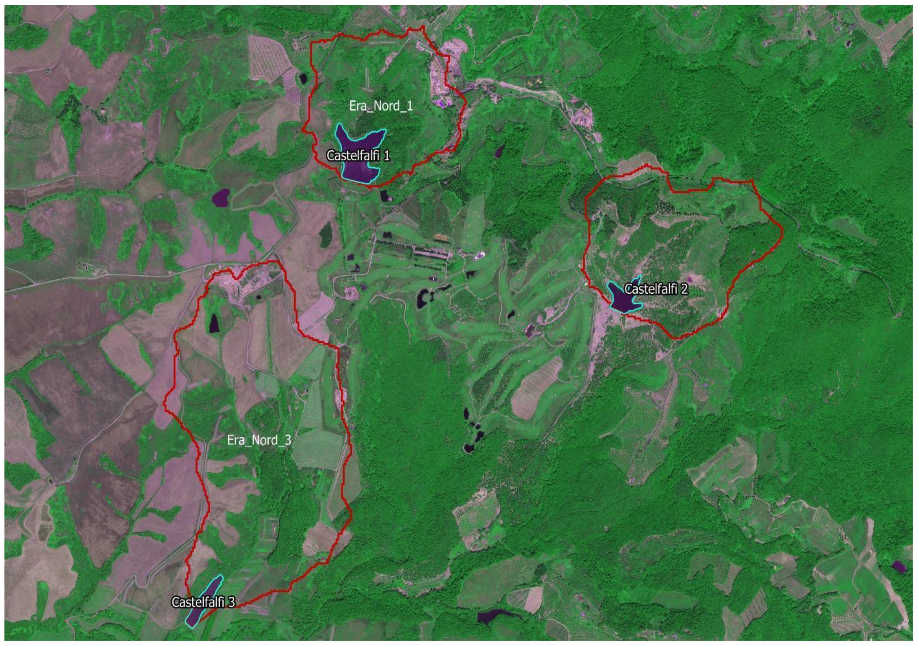
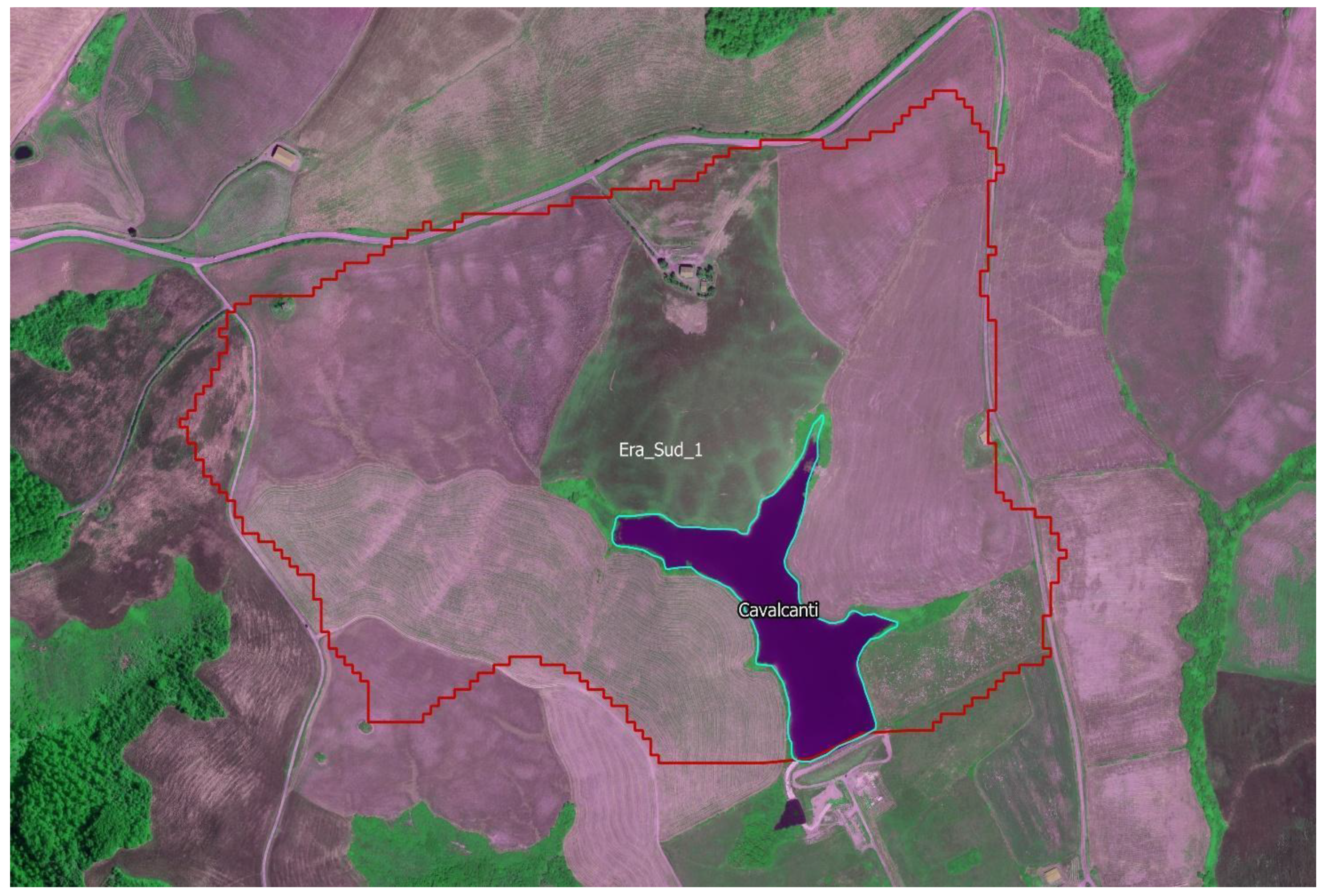
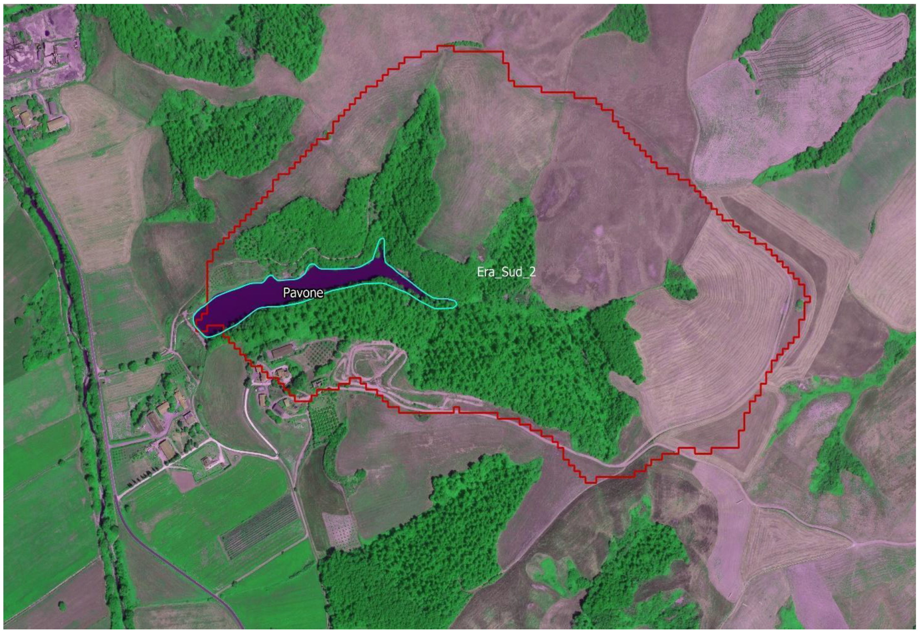
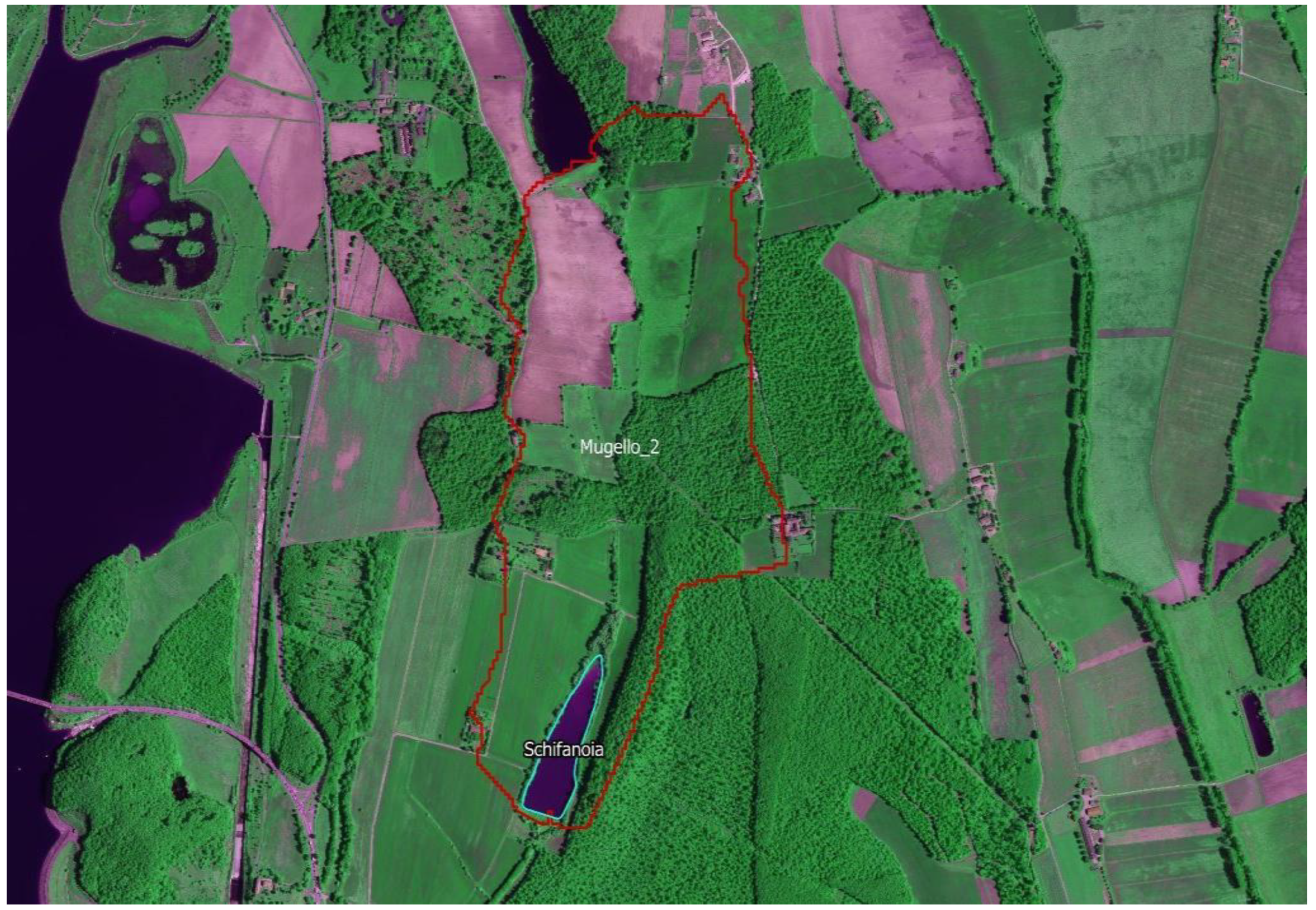
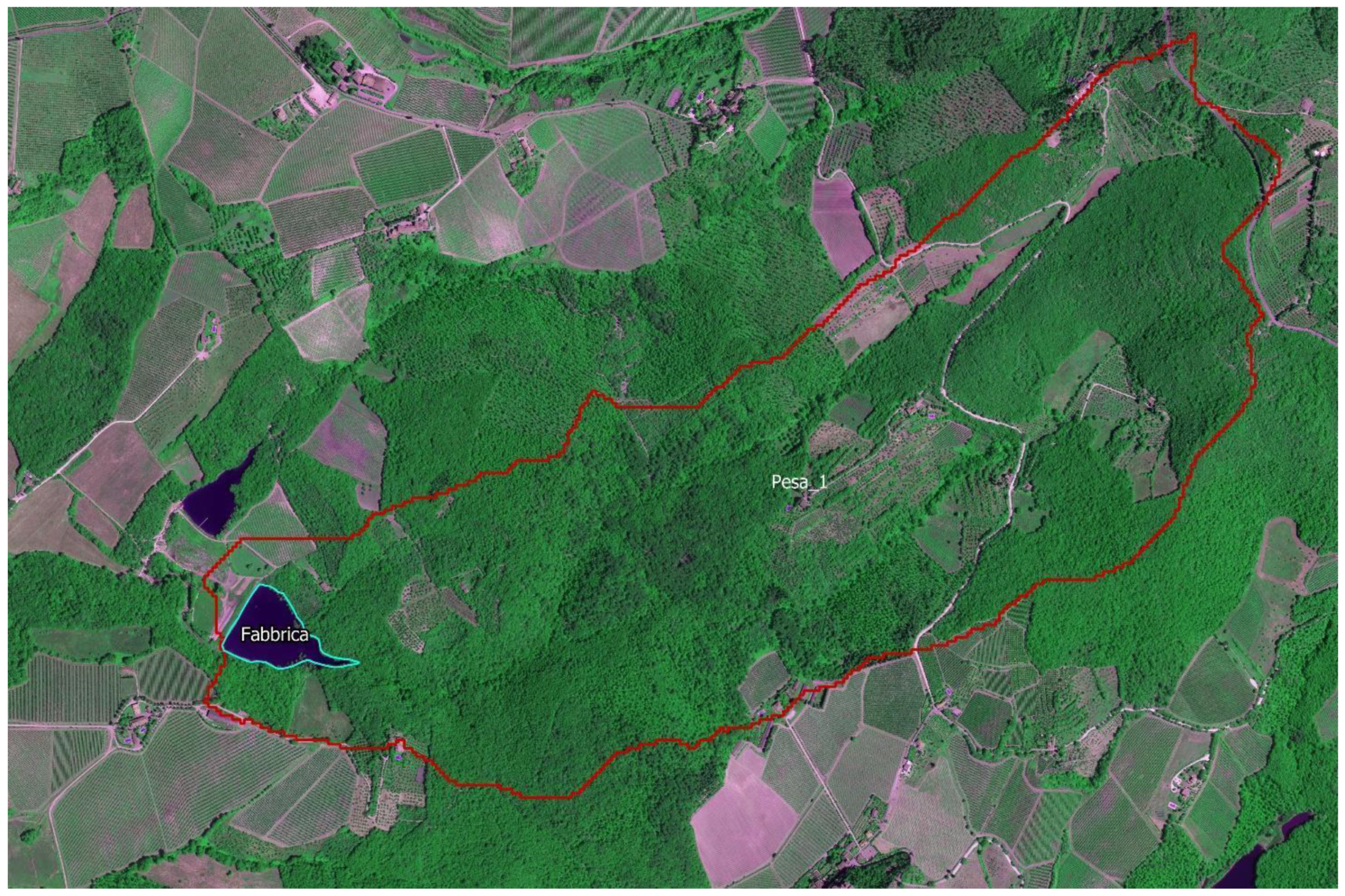
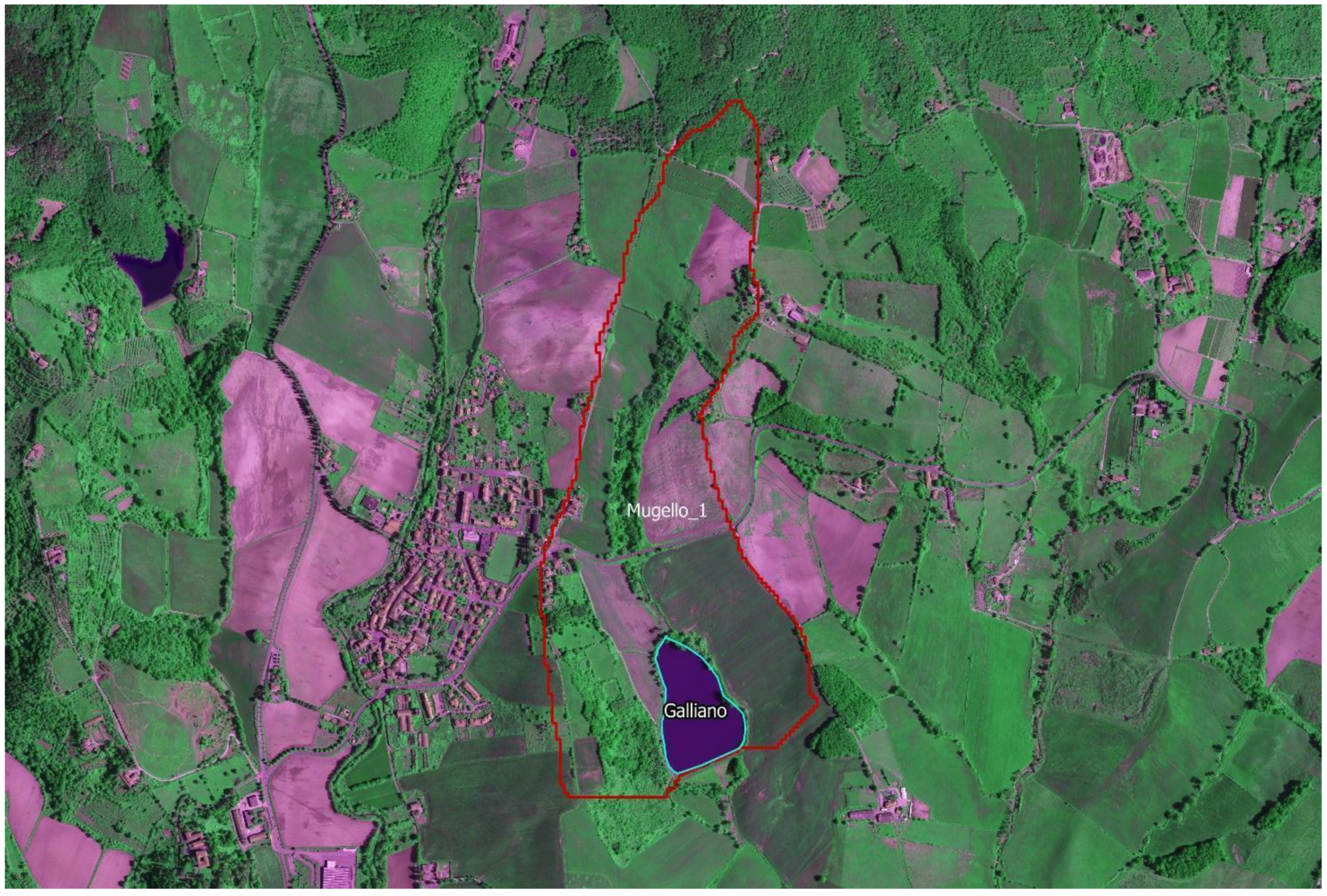
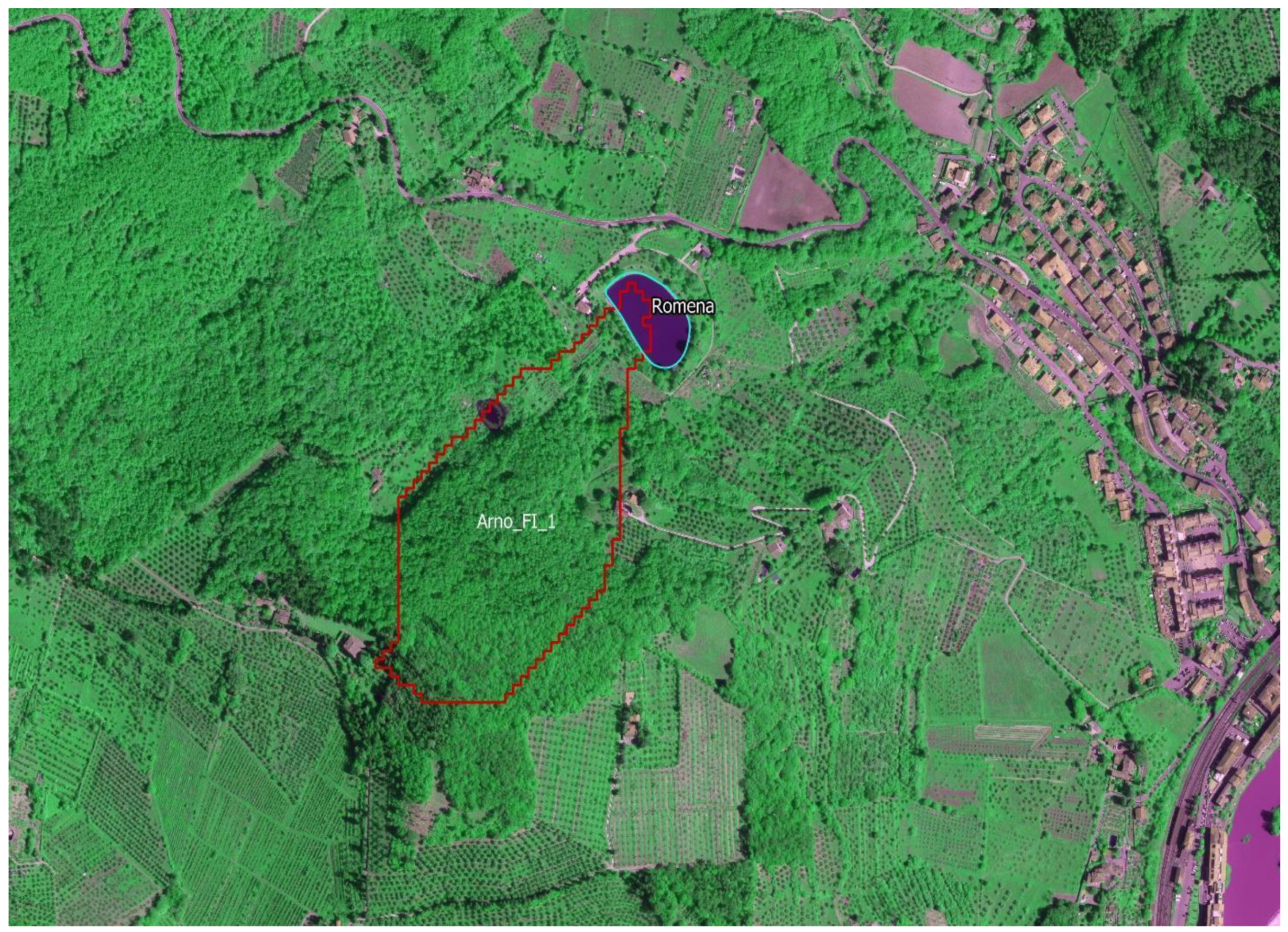
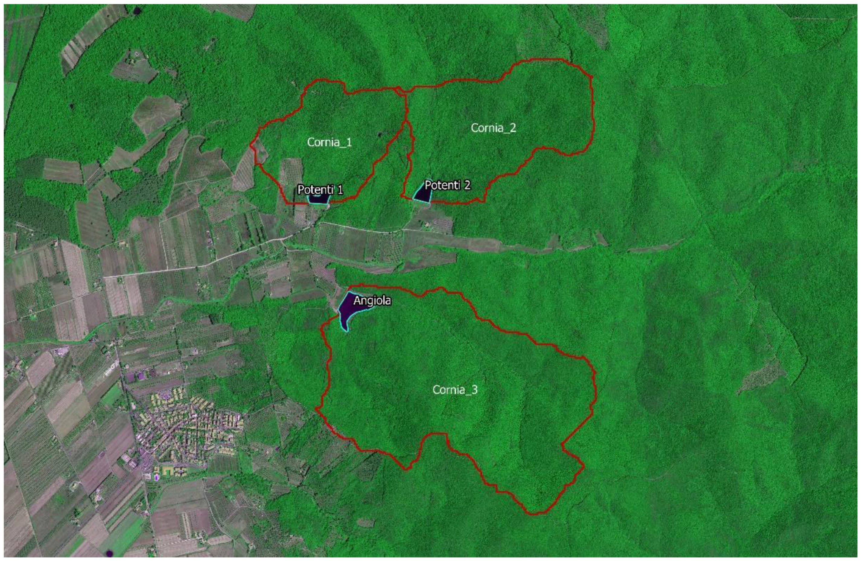
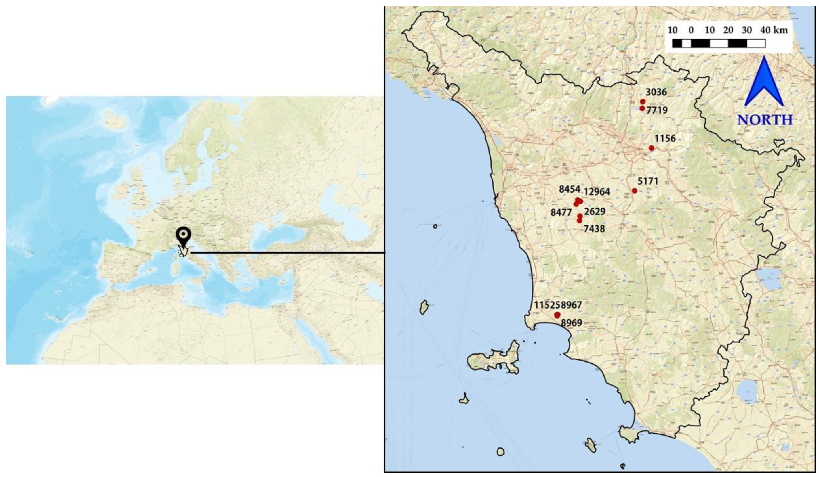
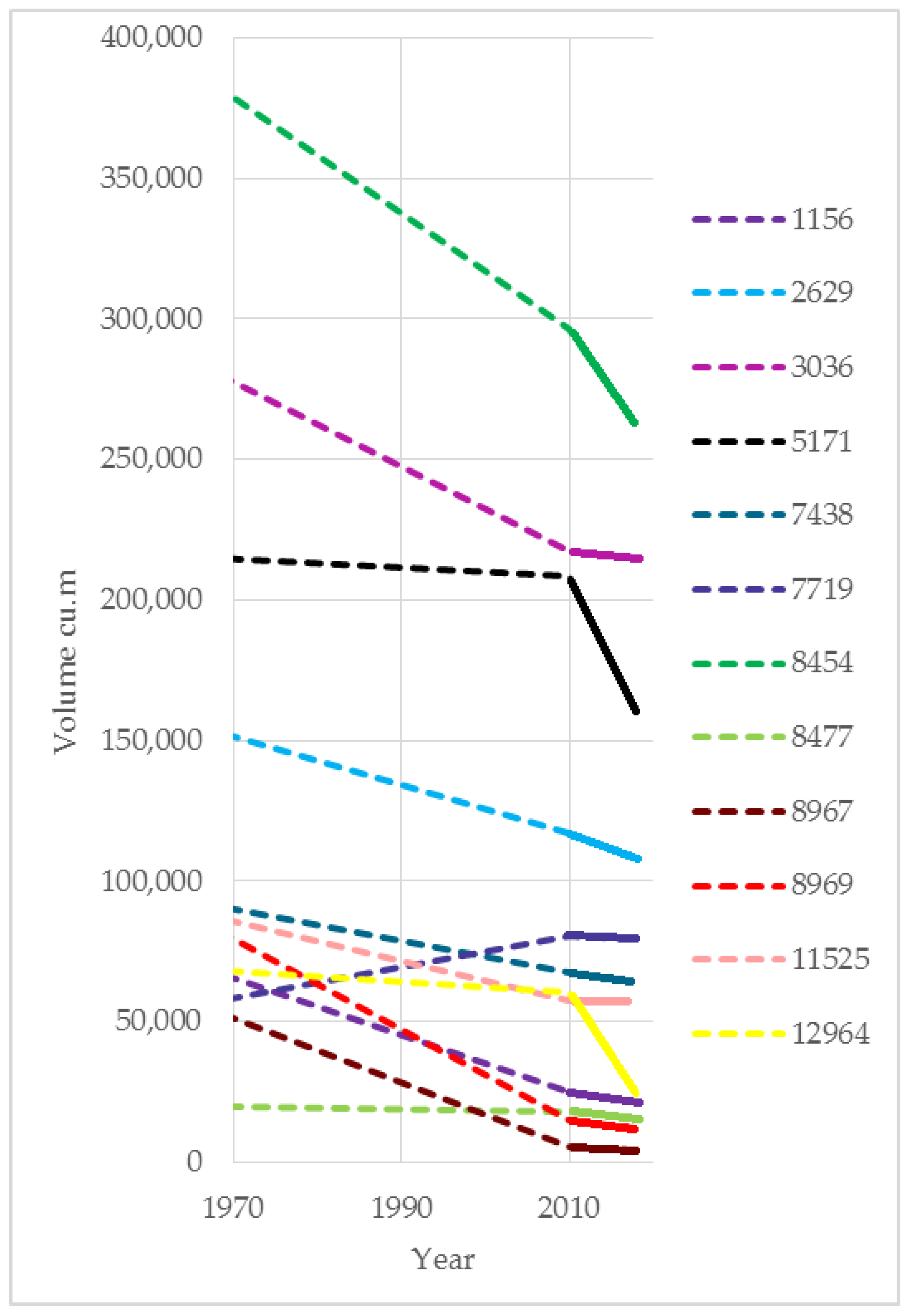
2.1. Lakes Analyzed and Volume Changes

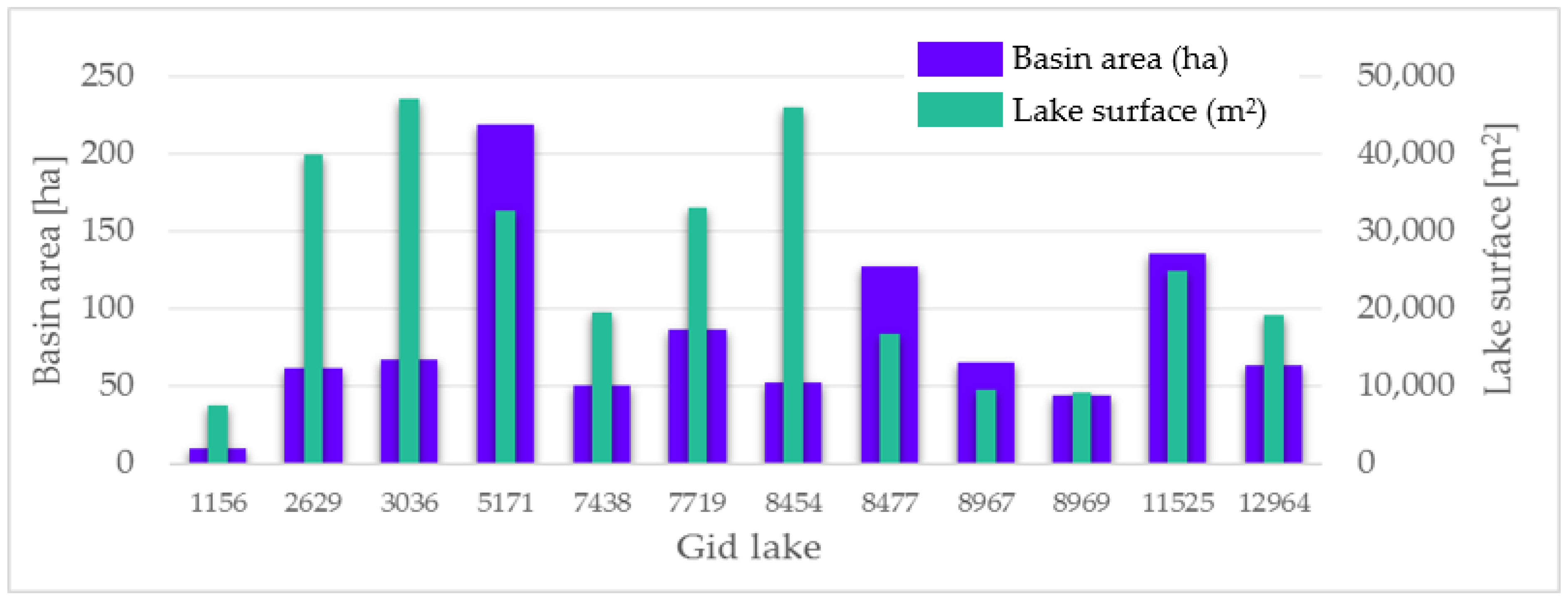
| GID | Lake Name | Area (ha) | Altitude Max (m agl) | Altitude Lake (m agl) | Slope Mean (%) | Hydrographic Network (m) | Road Network (m) |
|---|---|---|---|---|---|---|---|
| 1156 | Romena | 9.55 | 293 | 154 | 15.1 | 618.8 | 331.5 |
| 2629 | Cavalcanti | 61.64 | 212 | 156 | 10.9 | 2594.6 | 751.4 |
| 3036 | Galliano | 67.25 | 409 | 281 | 8.3 | 3515.7 | 2883.1 |
| 5171 | Fabbrica | 218.99 | 413 | 229 | 14.1 | 11,268.2 | 11,812.8 |
| 7438 | Pavone | 50.83 | 202 | 135 | 14.4 | 1998.9 | 1029.9 |
| 7719 | Schifanoia | 87.04 | 281 | 242 | 4.6 | 4549.5 | 2297.4 |
| 8454 | Castelfalfi 1 | 52.70 | 261 | 158 | 14.8 | 2459.3 | 4034.4 |
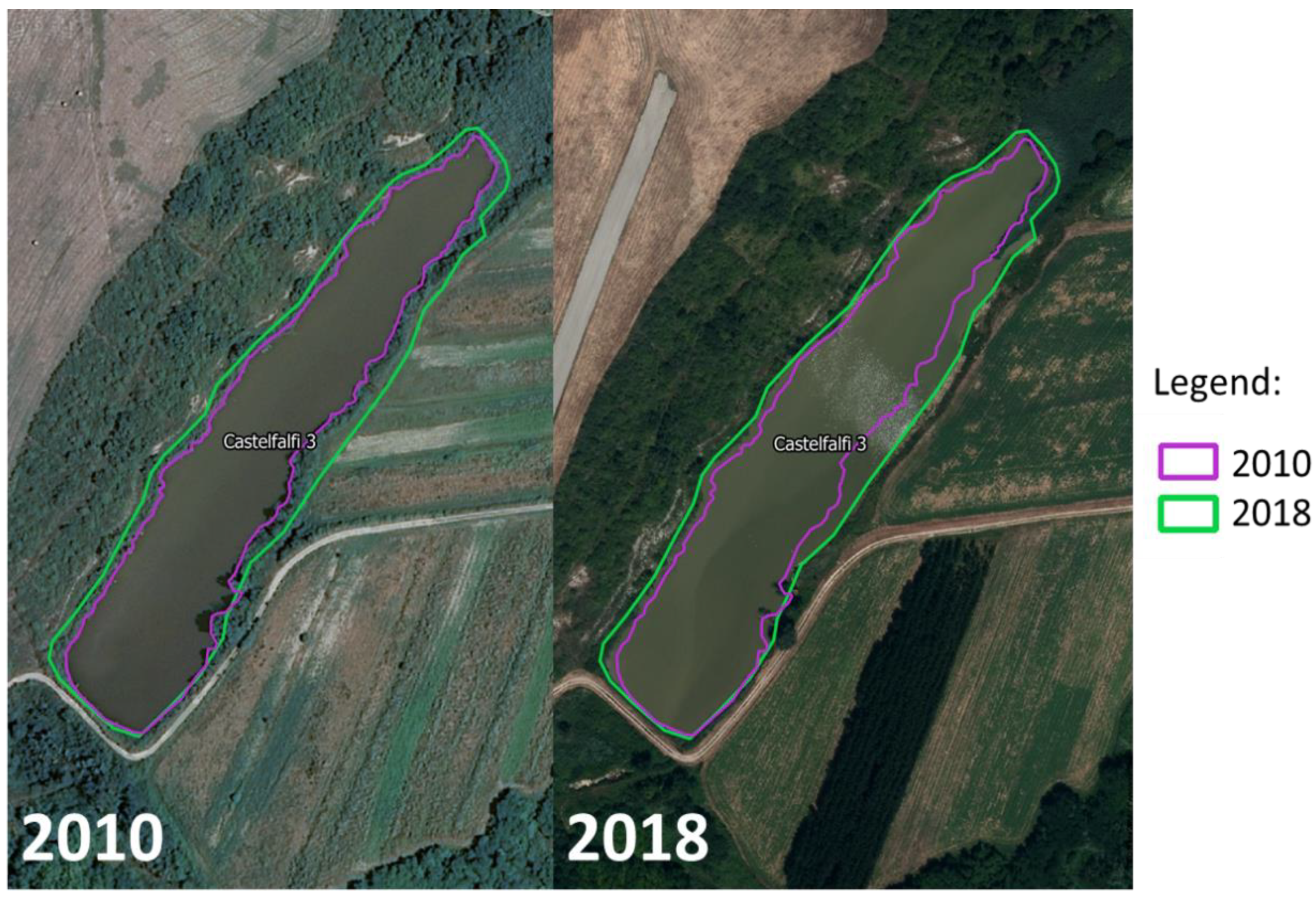
| 8477 | Castelfalfi 3 | 127.19 | 177 | 99 | 10.3 | 7852.2 | 6069.4 |
| 8967 | Potenti 2 | 65.34 | 183 | 48 | 11.5 | 4135.1 | 1091.1 |
| 8969 | Potenti 1 | 43.79 | 128 | 39 | 9.4 | 2351.5 | 0.0 |
| 11525 | Angiola | 136.16 | 195 | 35 | 14.6 | 8183.8 | 11,074.5 |
| 12964 | Castelfalfi 2 | 64.00 | 338 | 177 | 17.5 | 3507.2 | 1476.0 |
| GID | Construction Year | Volume of Design Phase (mc) |
|---|---|---|
| 1156 | 1964 | 76,000 |
| 2629 | 1958 | 160,000 |
| 3036 | 1958 | 293,150 |
| 5171 | 1956 | 216,420 |
| 7438 | 1959 | 96,000 |
| 7719 | 1970 | 52,500 |
| 8454 | 1970 | 400,000 |
| 8477 | 1963 | 20,507 |
| 8967 | 1970 | 63,000 |
| 8969 | 1970 | 96,000 |
| 11525 | 1970 | 93,000 |
| 12964 | 1967 | 69,803 |
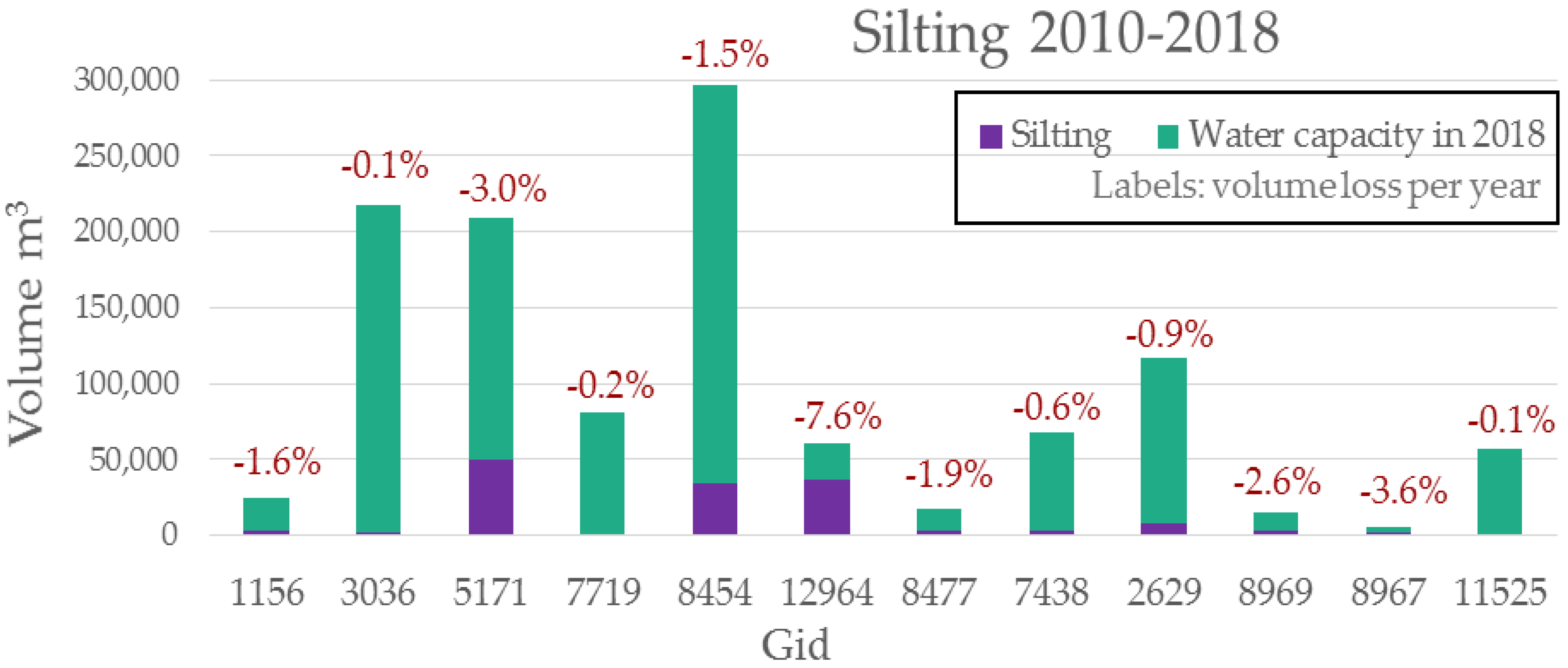
| Surface (m2) | Volume (m3) | Variation | Silting | ||||||
|---|---|---|---|---|---|---|---|---|---|
| GID | 2010 | 2018 | 2010-h | 2018 | m3 | % | %/y | Mg | Mg/y |
| 1156 | 7570 | 7599 | 24,855 | 21,597 | −3258 | −13.1 | −1.6 | 2821 | 353 |
| 2629 | 38,875 | 39,942 | 116,826 | 108,254 | −8572 | −7.3 | −0.9 | 7423 | 928 |
| 3036 | 49,986 | 47,241 | 217,520 | 215,144 | −2376 | −1.1 | −0.1 | 2057 | 257 |
| 5171 | 35,293 | 32,713 | 208,807 | 159,454 | −49,353 | −23.6 | −3.0 | 42,740 | 5342 |
| 7438 | 20,729 | 19,561 | 67,659 | 64,228 | −3431 | −5.1 | −0.6 | 2971 | 371 |
| 7719 | 35,080 | 33,029 | 80,651 | 79,407 | −1244 | −1.5 | −0.2 | 1077 | 135 |
| 8454 | 48,412 | 46,044 | 296,296 | 261,833 | −34,463 | −11.6 | −1.5 | 29,845 | 3731 |
| 8477 | 13,389 | 16,747 | 18,018 | 15,315 | −2703 | −15 | −1.9 | 2341 | 293 |
| 8967 | 8059 | 9654 | 5792 | 4141 | −1651 | −28.5 | −3.6 | 1430 | 179 |
| 8969 | 7744 | 9180 | 15,220 | 12,070 | −3150 | −20.7 | −2.6 | 2728 | 341 |
| 11525 | 21,246 | 24,886 | 57,625 | 57,238 | −387 | −0.7 | −0.1 | 335 | 42 |
| 12964 | 22,135 | 19,204 | 60,549 | 23,953 | −36,596 | −60.4 | −7.6 | 31,692 | 3961 |
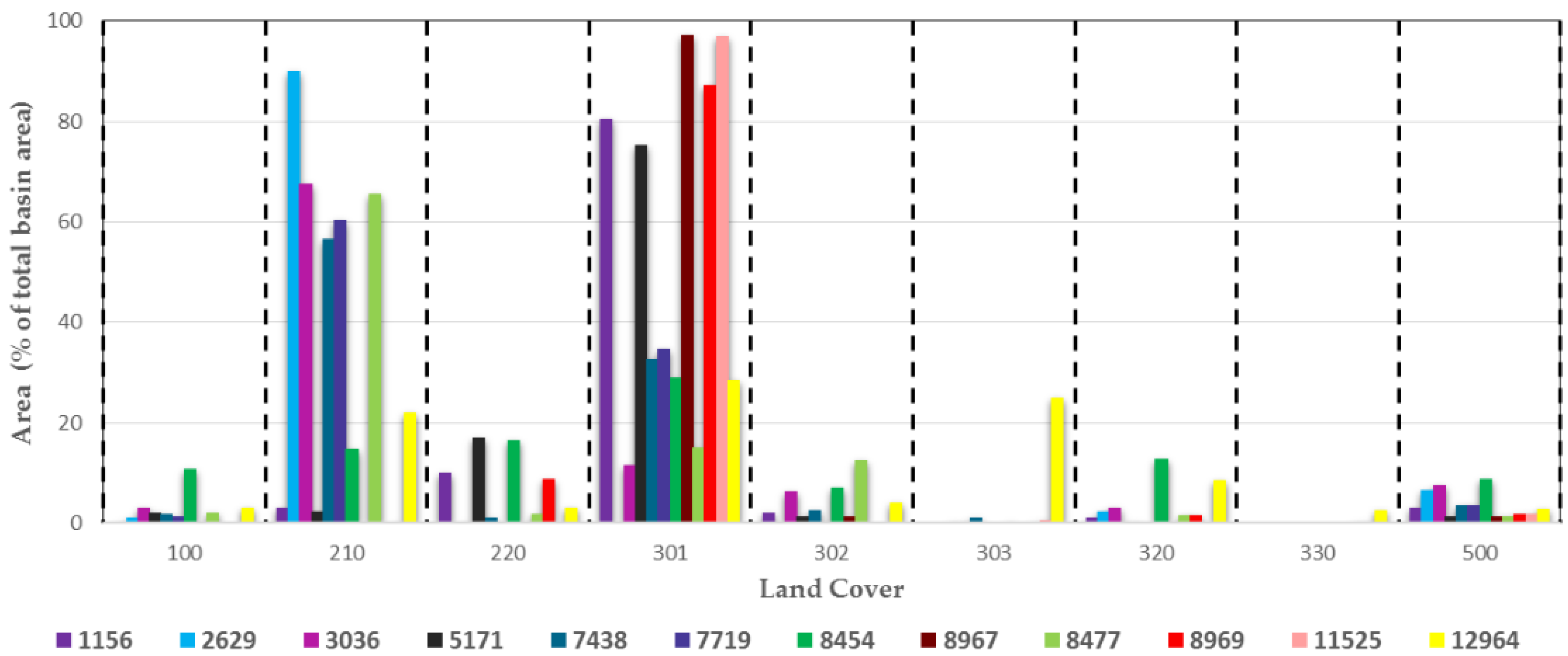
| UCS Code | Description | USLE_C | USLE_P |
|---|---|---|---|
| 100 | Artificial surfaces | 0 | 1 |
| 210 | Lands under a rotation system used for annually harvested plants and fallow lands | 0.15 | 1 |
| 220 | Permanent crops (vineyards and olive groves) | 0.4 | 1 |
| 301 | Forest with a complete canopy closure or a little less | 0.01 | 1 |
| 302 | Forest with a sparse canopy closure (40–60%), shrubs and max 10% of soil bare | 0.08 | 1 |
| 303 | Degraded forest (canopy closure less of 40%), shrubs cover of 40% and bare soil max 30% | 0.20 | 1 |
| 320 | Permanent shrub and/or herbaceous vegetation associations | 0.1 | 1 |
| 330 | Degraded soil or bare rock | 0.75 | 1 |
| 500 | Water bodies | 0 | 1 |
Harmonization
2.2. Erosion Simulation by the Morgan–Morgan–Finney Model
2.3. Erosion Estimate by RUSLE Model
Sediment Delivery Ratio
3. Results
4. Discussion
5. Conclusions
Author Contributions
Funding
Institutional Review Board Statement
Informed Consent Statement
Data Availability Statement
Acknowledgments
Conflicts of Interest
Appendix A


References
- Borrelli, P.; Robinson, D.A.; Panagos, P.; Lugato, E.; Yang, J.E.; Alewell, C.; Wuepper, D.; Montanarella, L.; Ballabio, C. Land use and climate change impacts on global soil erosion by water (2015–2070). Proc. Natl. Acad. Sci. USA 2020, 117, 21994–22001. [Google Scholar] [CrossRef]
- Pimentel, D. Soil erosion: A food and environmental threat. Environ. Dev. Sustain. 2006, 8, 119–137. [Google Scholar] [CrossRef]
- Pimentel, D.; Burgess, M. Soil erosion threatens food production. Agriculture 2013, 3, 443–463. [Google Scholar] [CrossRef] [Green Version]
- Pennock, D.; Pennock, L.; Sala, M. Soil Erosion: The Greatest Challenge for Soustainable Soil Management; Food & Agriculture Organization: Rome, Italy, 2019; ISBN 9789251314265. [Google Scholar]
- Pimentel, D.; Harvey, C.; Resosudarmo, P.; Sinclair, K.; Kurz, D.; McNair, M.; Crist, S.; Shpritz, L.; Fitton, L.; Saffouri, R.; et al. Environmental and economic costs of soil erosion and conservation benefits. Science 1995, 267, 1117–1123. [Google Scholar] [CrossRef] [PubMed] [Green Version]
- Kirkby, M.; Jones, R.J.; Irvine, B.; Gobin, A.G.G.; Cerdan, O.; van Rompaey, J.J.; Huting, J.R.M. Pan-European Soil Erosion Risk Assessment for Europe: The PESERA Map, version 1 October 2003; Office for Official Publications of the European Communities: Luxembourg, Germany, 2004. [Google Scholar]
- Nearing, M.A.; Foster, G.R.; Lane, L.J.; Finkner, S.C. A process-based soil erosion model for USDA-Water Erosion Prediction Project technology. Trans. ASAE 1989, 32, 1587–1593. [Google Scholar] [CrossRef]
- Laflen, J.; Lane, L.; Foster, G.R. WEPP: A new generation of erosion prediction technology. J. Soil Water Conserv. 1991, 46, 34–38. [Google Scholar]
- Assennato, F.; Antona, M.D.; Di Leginio, M.; Strollo, A. Assessing land consumption impact on ecosystem services provision: An insight on biophysical and economic dimension of loss of erosion control in Italy. Authorea 2020, 1–12. [Google Scholar] [CrossRef]
- Mastrorosa, S.; Crosetto, M.; Congedo, L.; Munafò, M. Land consumption monitoring: An innovative method integrating SAR and optical data. Environ. Monit. Assess. 2018, 190, 588. [Google Scholar] [CrossRef]
- Van Oost, K.; Bakker, M. Soil Productivity and Erosion. B Soil Ecol. Ecosyst. Serv. 2012, 2012, 301–314. [Google Scholar] [CrossRef]
- Stokes, A.; Douglas, G.B.; Fourcaud, T.; Giadrossich, F.; Gillies, C.; Hubble, T.; Kim, J.H.; Loades, K.W.; Mao, Z.; Mcivor, I.R.; et al. Ecological mitigation of hillslope instability: Ten key issues facing researchers and practitioners. Plant Soil 2014, 377, 1–23. [Google Scholar] [CrossRef] [Green Version]
- Fox, D.M.; Laaroussi, Y.; Malkinson, L.D.; Maselli, F.; Andrieu, J.; Bottai, L.; Wittenberg, L. POSTFIRE: A model to map forest fire burn scar and estimate runoff and soil erosion risks. Remote Sens. Appl. Soc. Environ. 2016, 4, 83–91. [Google Scholar] [CrossRef]
- Capra, G.F.; Ganga, A.; Grilli, E.; Vacca, S.; Buondonno, A. A review on anthropogenic soils from a worldwide perspective. J. Soils Sediments 2015, 15, 1602–1618. [Google Scholar] [CrossRef]
- SEC. Communication from the Commission to the Council, the European Parliament, the European Economic and Social Committee and the Committee of the Regions. In Thematic Strategy for Soil Protection; [SEC(2006)620], [SEC(2006)1165]; Communication from the Commission to the Council: Brussels, Belgium, 2006. [Google Scholar]
- Borrelli, P.; Robinson, D.A.; Fleischer, L.R.; Lugato, E.; Ballabio, C.; Alewell, C.; Meusburger, K.; Modugno, S.; Schütt, B.; Ferro, V.; et al. An assessment of the global impact of 21st century land use change on soil erosion. Nat. Commun. 2017, 8, 2013. [Google Scholar] [CrossRef] [Green Version]
- Caracciolo, C.; Napoli, M.; Porcù, F.; Prodi, F.; Dietrich, S.; Zanchi, C.; Orlandini, S. Raindrop Size Distribution and Soil Erosion. J. Irrig. Drain. Eng. 2012, 138, 461–469. [Google Scholar] [CrossRef]
- Napoli, M.; Marta, A.D.; Zanchi, C.A.; Orlandini, S. Assessment of soil and nutrient losses by runoff under different soil management practices in an Italian hilly vineyard. Soil Tillage Res. 2017, 168, 71–80. [Google Scholar] [CrossRef]
- Napoli, M.; Cecchi, S.; Orlandini, S.; Mugnai, G.; Zanchi, C.A. Simulation of field-measured soil loss in Mediterranean hilly areas (Chianti, Italy) with RUSLE. Catena 2016, 145, 246–256. [Google Scholar] [CrossRef]
- Canuti, P.; Moretti, S.; Bazzoffi, P.; Rodolfi, G.; Zanchi, C. Soil erosion as a result of the man activity-geological environment relationship an example of quantitative evaluation in the mugello valley (Tuscany, Italy). Bull. Int. Assoc. Eng. Geol. l’Assoc. Int. Géol. l’Ingénieur 1986, 33, 109–114. [Google Scholar] [CrossRef]
- Bagarello, V.; Iovino, M.; Elrick, D. A Simplified Falling-Head Technique for Rapid Determination of Field-Saturated Hydraulic Conductivity. Soil Sci. Soc. Am. J. 2004, 68, 66. [Google Scholar] [CrossRef]
- Vacca, A.; Loddo, S.; Ollesch, G.; Puddu, R.; Serra, G.; Tomasi, D.; Aru, A. Measurement of runoff and soil erosion in three areas under different land use in Sardinia (Italy). Catena 2000, 40, 69–92. [Google Scholar] [CrossRef]
- Wischmeier, W.; Smith, D. Predicting Rainfall Erosion Losses: A Guide to Conservation Planning; Agriculture Handbook (No. 537); United States Department of Agriculture: Washington, DC, USA, 1978; pp. 1–67. [Google Scholar]
- Renard, K.G. Predicting Soil Erosion by Water: A Guide to Conservation Planning with the Revised Universal Soil Loss Equation (RUSLE); Agriculture Handbook (No. 703); United States Department of Agriculture: Washington, DC, USA, 1997; p. 300. [Google Scholar]
- Poesen, J.; Nachtergaele, J.; Verstraeten, G.; Valentin, C. Gully erosion and environmental change: Importance and research needs. Catena 2003, 50, 91–133. [Google Scholar] [CrossRef]
- Renschler, C.S.; Harbor, J. Soil erosion assessment tools from point to regional scales—The role of geomorphologists in land management research and implementation. Geomorphology 2002, 47, 189–209. [Google Scholar] [CrossRef]
- Kinnell, P.I.A. Event soil loss, runoff and the Universal Soil Loss Equation family of models: A review. J. Hydrol. 2010, 385, 384–397. [Google Scholar] [CrossRef]
- Lu, H.; Prosser, I.P.; Moran, C.J.; Gallant, J.C.; Priestley, G.; Stevenson, J.G. Predicting sheetwash and rill erosion over the Australian continent. Aust. J. Soil Res. 2003, 41, 1037–1062. [Google Scholar] [CrossRef]
- Panagos, P.; Borrelli, P.; Meusburger, K. A new European slope length and steepness factor (LS-factor) for modeling soil erosion by water. Geosciences 2015, 5, 117–126. [Google Scholar] [CrossRef] [Green Version]
- Panagos, P.; Meusburger, K.; Ballabio, C.; Borrelli, P.; Alewell, C. Soil erodibility in Europe: A high-resolution dataset based on LUCAS. Sci. Total Environ. 2014, 479–480, 189–200. [Google Scholar] [CrossRef] [PubMed]
- Panagos, P.; Borrelli, P.; Meusburger, K.; Alewell, C.; Lugato, E.; Montanarella, L. Estimating the soil erosion cover-management factor at the European scale. Land Use Policy 2015, 48, 38–50. [Google Scholar] [CrossRef]
- Panagos, P.; Ballabio, C.; Borrelli, P.; Meusburger, K.; Klik, A.; Rousseva, S.; Tadić, M.P.; Michaelides, S.; Hrabalíková, M.; Olsen, P.; et al. Rainfall erosivity in Europe. Sci. Total Environ. 2015, 511, 801–814. [Google Scholar] [CrossRef] [Green Version]
- Benavidez, R.; Jackson, B.; Maxwell, D.; Norton, K. A review of the (Revised) Universal Soil Loss Equation ((R)USLE): With a view to increasing its global applicability and improving soil loss estimates. Hydrol. Earth Syst. Sci. 2018, 22, 6059–6086. [Google Scholar] [CrossRef] [Green Version]
- Alewell, C.; Borrelli, P.; Meusburger, K.; Panagos, P. Using the USLE: Chances, challenges and limitations of soil erosion modelling. Int. Soil Water Conserv. Res. 2019, 7, 203–225. [Google Scholar] [CrossRef]
- Le Roux, J.J.; Newby, T.S.; Sumner, P.D. Monitoring soil erosion in South Africa at a regional scale: Review and recommendations. S. Afr. J. Sci. 2007, 103, 329–335. [Google Scholar]
- Morgan, R.P.C.; Duzant, J.H. Modified MMF (Morgan–Morgan–Finney) model for evaluating effects of crops and vegetation cover on soil erosion. Earth Surf. Process. Landf. 2008, 32, 90–106. [Google Scholar] [CrossRef]
- Sterk, G. A hillslope version of the revised Morgan, Morgan and Finney water erosion model. Int. Soil Water Conserv. Res. 2021, 9, 319–332. [Google Scholar] [CrossRef]
- Li, C.; Qi, J.; Feng, Z.; Yin, R.; Guo, B.; Zhang, F.; Zou, S. Quantifying the effect of ecological restoration on soil erosion in china’s loess plateau region: An application of the MMF approach. Environ. Manag. 2010, 45, 476–487. [Google Scholar] [CrossRef]
- Tesfahunegn, G.B.; Tamene, L.; Vlek, P.L.G. Soil erosion prediction using Morgan-Morgan-Finney model in a GIS environment in northern Ethiopia catchment. Appl. Environ. Soil Sci. 2014, 2014, 468751. [Google Scholar] [CrossRef] [Green Version]
- Shrestha, D.P.; Jetten, V.G. Modelling erosion on a daily basis, an adaptation of the MMF approach. Int. J. Appl. Earth Obs. Geoinf. 2018, 64, 117–131. [Google Scholar] [CrossRef]
- Mondal, A.; Khare, D.; Kundu, S. A comparative study of soil erosion modelling by MMF, USLE and RUSLE. Geocarto Int. 2018, 33, 89–103. [Google Scholar] [CrossRef]
- Das, S.; Deb, P.; Bora, P.K.; Katre, P. Comparison of rusle and mmf soil loss models and evaluation of catchment scale best management practices for a mountainous watershed in india. Sustainability 2021, 13, 232. [Google Scholar] [CrossRef]
- Shen, Z.Y.; Gong, Y.W.; Li, Y.H.; Hong, Q.; Xu, L.; Liu, R.M. A comparison of WEPP and SWAT for modeling soil erosion of the Zhangjiachong Watershed in the Three Gorges Reservoir Area. Agric. Water Manag. 2009, 96, 1435–1442. [Google Scholar] [CrossRef]
- Mosbahi, M.; Benabdallah, S.; Boussema, M.R. Assessment of soil erosion risk using SWAT model. Arab. J. Geosci. 2013, 6, 4011–4019. [Google Scholar] [CrossRef]
- Tibebe, D.; Bewket, W. Surface runoff and soil erosion estimation using the SWAT model in the Keleta Watershed, Ethiopia. Land Degrad. Dev. 2011, 22, 551–564. [Google Scholar] [CrossRef]
- Napoli, M.; Orlandini, S.; Grifoni, D.; Zanchi, C.A. Modelling soil and nutrient runoff yields from an Italian vineyards using swat. Trans. ASABE 2013, 56, 1397–1406. [Google Scholar]
- Pacetti, T.; Castelli, G.; Schröder, B.; Bresci, E.; Caporali, E. Water Ecosystem Services Footprint of agricultural production in Central Italy. Sci. Total Environ. 2021, 797, 149095. [Google Scholar] [CrossRef] [PubMed]
- Castelli, G.; Foderi, C.; Guzman, B.H.; Ossoli, L.; Kempff, Y.; Bresci, E.; Salbitano, F. Planting waterscapes: Green infrastructures, landscape and hydrological modeling for the future of Santa Cruz de la Sierra, Bolivia. Forests 2017, 8, 437. [Google Scholar] [CrossRef] [Green Version]
- Bagarello, V.; Di Piazza, G.; Ferro, V.; Giordano, G. Predictiong unit plot soil loss in Sicily, south Italy. Hydrol. Process. 2008, 22, 586–595. [Google Scholar] [CrossRef]
- Bagarello, V.; Ferro, V.; Keesstra, S.; Comino, J.R.; Pulido, M.; Cerdà, A. Testing simple scaling in soil erosion processes at plot scale. Catena 2018, 167, 171–180. [Google Scholar] [CrossRef]
- Wu, S.; Chen, L.; Wang, N.; Zhang, J.; Wang, S.; Bagarello, V.; Ferro, V. Variable scale effects on hillslope soil erosion during rainfall-runoff processes. Catena 2021, 207, 105606. [Google Scholar] [CrossRef]
- Angeli, L.; Bottai, L.; Costantini, R.; Ferrari, R.; Innocenti, L.; Märker, M. Carta della suscettibiltià all’erosione: Analisi e confronto fra modelli di erosione del suolo. Atti ASITA 2009. Available online: http://atti.asita.it/Asita2005/Pdf/0223.pdf (accessed on 29 March 2022).
- ISPRA. Stato dell’Ambiente—Annuario dei Dati Ambientali; Geosfera 13/2009 1-23; ISPRA: Roma, Italy, 2016. [Google Scholar]
- Zanchi, C.A. Primi risultati sperimentali sull’influenza di differenti colture nei confronti del ruscellamento superficiale e dell’erosione. In Annali dell’Istituto Sperimentale per lo Studio e la Difesa del Suolo; Autorità di Bacino del Fiume Arno: Firenze, Italy, 1983; Volume XIV, pp. 277–289. [Google Scholar]
- Zanchi, C.A. Influenza dell’azione battente della pioggia e del ruscellamento nel processo erosivo e variazioni dell’erodibilità del suolo nei diversi periodi stagionali. In Annali dell’Istituto Sperimentale per lo Studio e la Difesa del Suolo; Autorità di Bacino del Fiume Arno: Firenze, Italy, 1983; Volume 14, pp. 347–358. [Google Scholar]
- Rodolfi, G.; Zanchi, C. Caratteristiche fondamentali e dinamica del paesaggio dell’Appennino Tosco Romagnolo. In Annali dell’Istituto Sperimentale per lo Studio e la Difesa del Suolo; Autorità di Bacino del Fiume Arno: Firenze, Italy, 1983; Volume XIV, pp. 289–336. [Google Scholar]
- Giambastiani, Y.; Giusti, R.; Cecchi, S.; Palomba, F.; Manetti, F.; Romanelli, S.; Bottai, L. Volume estimation of lakes and reservoirs based on aquatic drone surveys: The case study of Tuscany, Italy. J. Water Land Dev. 2020, 46, 84–96. [Google Scholar] [CrossRef]
- Schweizer, S.; Pini Prato, E. Gestione e tutela (applicazione direttiva nitrati) delle risorse idriche e valutazione degli approvvigionamenti nel settore agricolo ed elaborazione di cartografia tematica (gis) sulle risorse idriche ad uso irriguo. ARSIA—Reg. Toscana 2010, 1, 1–41. [Google Scholar]
- Fernández, C.; Vega, J.A.; Vieira, D.C.S. Assessing soil erosion after fire and rehabilitation treatments in NW Spain: Performance of rusle and revised Morgan-Morgan-Finney models. Land Degrad. Dev. 2010, 21, 58–67. [Google Scholar] [CrossRef] [Green Version]
- Giannetti, F.; Pegna, R.; Francini, S.; McRoberts, R.E.; Travaglini, D.; Marchetti, M.; Mugnozza, G.S.; Chirici, G. A new method for automated clearcut disturbance detection in mediterranean coppice forests using landsat time series. Remote Sens. 2020, 12, 3720. [Google Scholar] [CrossRef]
- Borselli, L.; Cassi, P.; Sanchis, P.S.; Ungaro, F.; Menduni, G.; Brugioni, M.; Sulli, L.; Montini, G. Studio della Dinamica delle Aree Sorgenti Primarie di Sedimento Nell’area Pilota del Bacino di Bilancino: Progetto (BABI); Relazione Attività di Progetto; Autorità di Bacino del Fiume Arno: Firenze, Italy, 2007. [Google Scholar] [CrossRef]
- Desmet, P.J.J.; Govers, G. GIS-based simulation of erosion and deposition patterns in an agricultural landscape: A comparison of model results with soil map information. Catena 1995, 25, 389–401. [Google Scholar] [CrossRef]
- Oliveira, A.H.; da Silva, M.A.; Silva, M.L.N.; Curi, N.; Neto, G.K.; de Freitas, D.A.F. Development of Topographic Factor Modeling for Application in Soil Erosion Models; InTech: London, UK, 2013; pp. 111–138. [Google Scholar]
- Bazzoffi, P. Erosione del Suolo e Sviluppo Rurale Sostenibile. Fondamenti e Manualistica per la Valutazione Agroambientale; Il Sole 24 Ore Edagricole: Milan, Italy, 2007; ISBN 8850652283. [Google Scholar]
- Borselli, L.; Cassi, P.; Torri, D. Prolegomena to sediment and flow connectivity in the landscape: A GIS and field numerical assessment. Catena 2008, 75, 268–277. [Google Scholar] [CrossRef]
- Rajbanshi, J.; Bhattacharya, S. Assessment of soil erosion, sediment yield and basin specific controlling factors using RUSLE-SDR and PLSR approach in Konar river basin, India. J. Hydrol. 2020, 587, 124935. [Google Scholar] [CrossRef]
- Vanoni, V.A. Sedimentation Engineering; American Society of Civil Engineers: New York, NY, USA, 1975; 745p. [Google Scholar]
- Ferro, V.; Porto, P. Sediment delivery distributed (sedd) model. J. Hydrol. Eng. 2000, 5, 411–422. [Google Scholar] [CrossRef]
- Saygın, S.D.; Ozcan, A.U.; Basaran, M.; Timur, O.B.; Dolarslan, M.; Yılman, F.E.; Erpul, G. The combined RUSLE/SDR approach integrated with GIS and geostatistics to estimate annual sediment flux rates in the semi-arid catchment, Turkey. Environ. Earth Sci. 2014, 71, 1605–1618. [Google Scholar] [CrossRef]
- Li, P.; Mu, X.; Holden, J.; Wu, Y.; Irvine, B.; Wang, F.; Gao, P.; Zhao, G.; Sun, W. Comparison of soil erosion models used to study the Chinese Loess Plateau. Earth-Sci. Rev. 2017, 170, 17–30. [Google Scholar] [CrossRef] [Green Version]
- Angeli, L.; Costantini, R.; Costanza, L.; Ferrari, R.; Gardin, L.; Innocenti, L. Rapporto Finale Ufficiale Sulla Realizzazione Della “Carta del Rischio di Erosione Idrica Attuale Della Regione Toscana in Scala 1:250.000”—Region Toscana; Consorzio LaMMA: Sesto Fiorentino, Italy, 2004. [Google Scholar]
- Tauro, F.; Petroselli, A.; Fiori, A.; Romano, N.; Rulli, M.C.; Porfiri, M.; Palladino, M.; Grimaldi, S. “Cape Fear”-A hybrid hillslope plot for monitoring hydrological processes. Hydrology 2017, 4, 35. [Google Scholar] [CrossRef] [Green Version]
- Tazioli, A. Evaluation of erosion in equipped basins: Preliminary results of a comparison between the Gavrilovic model and direct measurements of sediment transport. Environ. Geol. 2009, 56, 825–831. [Google Scholar] [CrossRef]
- Romano, N.; Nasta, P.; Bogena, H.; De Vita, P.; Stellato, L.; Vereecken, H. Monitoring Hydrological Processes for Land and Water Resources Management in a Mediterranean Ecosystem: The Alento River Catchment Observatory. Vadose Zone J. 2018, 17, 180042. [Google Scholar] [CrossRef] [Green Version]


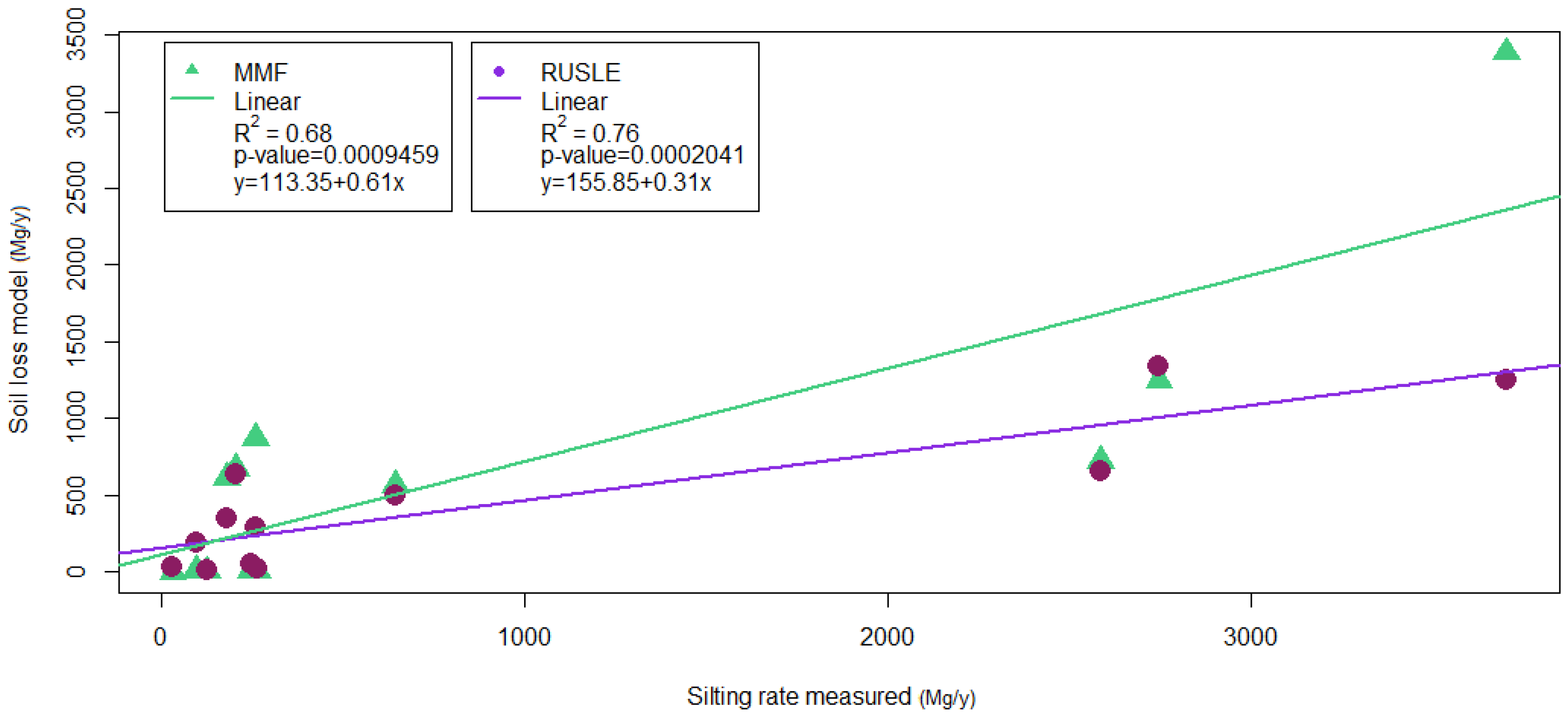
| GID Lake | Basin Area (ha) | Silting (Mg/y) | SL RUSLE (Mg/y) | SL MMF (Mg/y) | Silting (Mg y−1 ha−1) | RUSLE (Mg y−1 ha−1) | MMF (Mg y−1 ha−1) |
|---|---|---|---|---|---|---|---|
| 1156 | 10 | 244 | 49 | 4 | 24.393 | 4.928 | 0.422 |
| 2629 | 60 | 643 | 499 | 559 | 10.703 | 8.306 | 9.299 |
| 3036 | 81 | 178 | 344 | 609 | 2.197 | 4.242 | 7.511 |
| 5171 | 213 | 3701 | 1248 | 3384 | 17.390 | 5.862 | 15.900 |
| 7438 | 50 | 257 | 290 | 871 | 5.183 | 5.842 | 17.543 |
| 7719 | 101 | 93 | 192 | 7 | 0.925 | 1.899 | 0.071 |
| 8454 | 41 | 2585 | 655 | 721 | 63.529 | 16.092 | 17.733 |
| 8477 | 106 | 203 | 630 | 675 | 1.906 | 5.925 | 6.349 |
| 8967 | 53 | 124 | 11 | 3 | 2.341 | 0.209 | 0.049 |
| 8969 | 32 | 236 | 17 | 3 | 7.329 | 0.523 | 0.088 |
| 11525 | 135 | 29 | 31 | 1 | 0.215 | 0.229 | 0.004 |
| 12964 | 60 | 2745 | 1342 | 1247 | 45.475 | 22.231 | 20.653 |
Publisher’s Note: MDPI stays neutral with regard to jurisdictional claims in published maps and institutional affiliations. |
© 2022 by the authors. Licensee MDPI, Basel, Switzerland. This article is an open access article distributed under the terms and conditions of the Creative Commons Attribution (CC BY) license (https://creativecommons.org/licenses/by/4.0/).
Share and Cite
Giambastiani, Y.; Giusti, R.; Gardin, L.; Cecchi, S.; Iannuccilli, M.; Romanelli, S.; Bottai, L.; Ortolani, A.; Gozzini, B. Assessing Soil Erosion by Monitoring Hilly Lakes Silting. Sustainability 2022, 14, 5649. https://doi.org/10.3390/su14095649
Giambastiani Y, Giusti R, Gardin L, Cecchi S, Iannuccilli M, Romanelli S, Bottai L, Ortolani A, Gozzini B. Assessing Soil Erosion by Monitoring Hilly Lakes Silting. Sustainability. 2022; 14(9):5649. https://doi.org/10.3390/su14095649
Chicago/Turabian StyleGiambastiani, Yamuna, Riccardo Giusti, Lorenzo Gardin, Stefano Cecchi, Maurizio Iannuccilli, Stefano Romanelli, Lorenzo Bottai, Alberto Ortolani, and Bernardo Gozzini. 2022. "Assessing Soil Erosion by Monitoring Hilly Lakes Silting" Sustainability 14, no. 9: 5649. https://doi.org/10.3390/su14095649
APA StyleGiambastiani, Y., Giusti, R., Gardin, L., Cecchi, S., Iannuccilli, M., Romanelli, S., Bottai, L., Ortolani, A., & Gozzini, B. (2022). Assessing Soil Erosion by Monitoring Hilly Lakes Silting. Sustainability, 14(9), 5649. https://doi.org/10.3390/su14095649